Road Network Capacity Assessment and Improvement Strategies for Bimodal Urban Networks Based on the Three-Dimensional Macroscopic Fundamental Diagram

Featured Application

The proposed 3D-MFD-based simulation-statistical framework can support parameter screening for bus-lane allocation and bus-fleet management in bimodal urban traffic networks.

Abstract

Urban congestion is difficult to alleviate through road expansion alone, making it necessary to improve existing road-network performance while maintaining public-transport priority. Under transit-priority policies, buses and private vehicles share limited road space, and bus lanes, stops, and lane-changing interactions may either improve or reduce network efficiency. This study treats capacity improvement as a constrained network-performance objective that preserves feasible bus operation and supports higher-occupancy, lower-emission public transport. A simulation-based capacity evaluation framework was developed using the three-dimensional macroscopic fundamental diagram (3D-MFD). A grid network was built in Simulation of Urban Mobility (SUMO), and 16 scenarios were designed by varying four factors: dedicated bus-lane proportion, average bus dwell time, driver lane-changing willingness, and bus-to-private-vehicle ratio. The 3D-MFD was fitted by nonlinear least squares, and range analysis and analysis of variance were used to identify significant factors. Results show that bus-lane proportion and bus-to-private-vehicle ratio dominate capacity variation. A supplementary simulation-based transferability assessment on a Beijing subnetwork further showed that the 4% bus-lane share and 7% bus-to-private-vehicle ratio produced the highest tested capacity response. The findings provide an assumption-bounded basis for screening bus-priority parameters rather than universal design values.

1. Introduction

Urban road networks are essential infrastructure for daily mobility and socioeconomic activity. With continuing urbanization and motorization, many cities face severe congestion while the physical expansion of road infrastructure remains increasingly constrained [1,2]. Under these conditions, improving the carrying capacity of existing networks has become a practical problem for traffic governance and sustainable urban development.

Road network capacity describes the maximum traffic load that a network can accommodate while maintaining an acceptable operating state. Capacity analysis supports the identification of bottlenecks, the diagnosis of operational risks, and the formulation of infrastructure and management strategies [3]. Because public transport can move more passengers with less road space per passenger, bus-priority policies are widely adopted as a means of improving system efficiency [4]. Nevertheless, dedicated bus lanes, bus stops, and bus dwell operations may also reduce the effective space and continuity available to private vehicles. Hence, the performance of buses and private vehicles should be analyzed as an interacting bimodal system rather than as two independent subsystems [5].

From a social-optimization perspective, the objective of capacity management should not be reduced to moving the largest possible number of private vehicles. Urban road space is scarce, and buses generally provide substantially higher passenger movement per unit of road space than private cars. Therefore, the capacity objective in this paper is used as an operational constraint for balancing two goals: maintaining network stability under mixed traffic and preserving sufficient bus service so that public transport can remain an attractive and environmentally preferable mode. This interpretation is consistent with recent multimodal MFD applications that evaluate road-space investment, pricing, and public-transport priority at the network level [6,7].

Existing capacity-estimation methods include the time-space consumption method, maximum-flow/minimum-cut analysis, traffic assignment models, bi-level programming, and macroscopic fundamental diagram-based approaches. Time-space consumption and network-flow methods provide useful structural or operational indicators but are often sensitive to local survey conditions or insufficiently dynamic [8,9]. Network design and assignment models can represent route choice and supply–demand interaction, although their tractability may decline in complex urban networks [10]. MFD-based methods provide a macroscopic relationship between accumulation and production/flow and are therefore suitable for network-level capacity diagnosis [11].

The conventional two-dimensional MFD has been widely used to investigate network shape, existence conditions, influencing factors, and control applications [12,13,14,15,16,17,18,19]. However, a two-dimensional MFD is usually formulated for a single dominant traffic mode and cannot explicitly represent the interaction between buses and private vehicles. Geroliminis et al. [20] extended the MFD to a three-dimensional form for mixed bimodal networks by relating car accumulation, bus accumulation, and network flow. Subsequent studies have further demonstrated the value of multimodal and 3D-MFD concepts for characterizing network performance and public-transport priority effects [21,22,23,24,25,26,27,28,29].

Despite these advances, three issues remain insufficiently developed for practical capacity management. First, most 3D-MFD studies use the surface primarily as a descriptive representation of multimodal traffic states, whereas its use for extracting a capacity threshold and screening implementable policy parameters remains limited. Second, the quantitative effects of bus-lane proportion, bus dwell time, bus-to-private-vehicle ratio, and lane-changing behavior on the capacity threshold have not been systematically compared within a unified simulation and statistical framework. Third, many 3D-MFD applications focus on idealized or single-network demonstrations; additional transferability checks on real-city topologies are still needed before the method can be used as an applied planning support tool. These gaps are important because bimodal capacity is not simply the sum of bus capacity and private-vehicle capacity; it depends on how bus-priority facilities, bus-stop operations, and lane-changing interactions redistribute limited road space and reshape the network-level flow response.

To address these gaps, this study develops a 3D-MFD-based procedure for assessing and improving road network capacity under bimodal traffic conditions. The objectives are: (i) to construct a reproducible SUMO simulation platform for a grid-based bimodal network; (ii) to estimate a vehicle-based 3D-MFD surface using bus and private-vehicle accumulations and network flow; (iii) to identify key capacity-influencing factors through orthogonal experimental design, range analysis, and ANOVA; and (iv) to assess the transferability of the resulting parameter combination in a more heterogeneous Beijing subnetwork simulation. Compared with previous 3D-MFD-based studies, the scientific novelty lies in coupling 3D-MFD capacity extraction with orthogonal statistical screening and then testing whether the selected parameter combination remains plausible in a real-city subnetwork, rather than claiming a universal optimum from a single simulated surface.

The remainder of this paper is organized as follows. Section 2 presents the overall methodology, including the 3D-MFD formulation and the statistical analysis framework. Section 3 describes the SUMO case study, capacity estimation, orthogonal experiments, strategy analysis, and simulation-based transferability assessment. Section 4 discusses the implications and limitations. Section 5 concludes the paper.

2. Methodology

This section describes the methodological framework used to evaluate road network capacity and to screen capacity-improvement strategies. The procedure consists of 3D-MFD formulation, capacity definition, SUMO-based data generation, and statistical factor analysis.

2.1. Research Framework

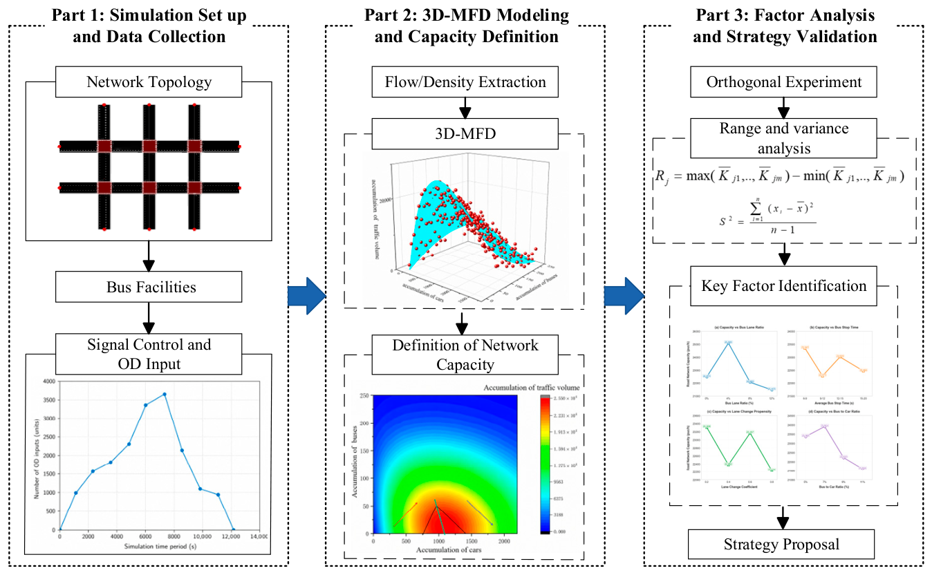
The proposed framework contains three modules, as illustrated in Figure 1. The first module constructs a controllable bimodal traffic simulation environment and generates reproducible traffic-flow data. The second module extracts the accumulation of private vehicles, the accumulation of buses, and the total network flow to estimate the 3D-MFD surface and define the capacity indicator. The third module applies orthogonal experiments, range analysis, and ANOVA to identify the dominant factors affecting capacity and to formulate parameter-based improvement strategies.

In the simulation module, a grid-based road network is built in SUMO with bus stops, dedicated bus lanes, signal control, and origin-destination (OD) demand. In the 3D-MFD module, interval-based edge outputs are aggregated to obtain mode-specific accumulations and network flow. In the factor-analysis module, the effects of bus-lane proportion, bus dwell time, bus-to-private-vehicle ratio, and lane-changing willingness are compared through a 16-scenario orthogonal design.

2.2. Three-Dimensional Macroscopic Fundamental Diagram

2.2.1. Theoretical Basis of the 3D-MFD

The 3D-MFD extends the conventional MFD by explicitly distinguishing the accumulations of two interacting modes. Following the vehicle-based 3D-MFD concept proposed for mixed bimodal networks [20], the network state is represented by the accumulation of private vehicles, the accumulation of buses, and the corresponding circulating network flow. This representation is suitable for examining how bus operations and private-vehicle operations jointly determine network-level performance.

For mode m, the mode-specific accumulation and circulating flow are computed from link-level density, length, and flow, as shown in Equation (1).

$$\left\{\begin{array}{c}{N}_m={\displaystyle \sum _i}{k}_{im}{l}_i\\ Q_m={\displaystyle \frac{{\sum }_i{q}_{im}{l}_i}{l}}\\ Q={\displaystyle \sum _m}{Q}_m\\ V={\displaystyle \frac{QL}{{\sum }_m{N}_m}}\\ m\in \left\{\left.b,c\right\}\right.\end{array}\right.$$

(1)

where $N_m$ is the cumulative number of vehicles of mode $m$ in the road network, with the unit of vehicles, $k_{im}$ is the vehicle density of mode m on road segment $i$, $l_i$ is the length of link $i$, $Q_m$ is the circulating flow of mode $m$, $q_{im}$ is the link flow, $L$ is the average link length, $V$ is the mean network speed, and $m\in \{\mathrm{b},\mathrm{c}\}$, where $b$ denotes buses and $c$ denotes private vehicles. The total network flow $Q$ is the sum of bus flow and private-vehicle flow.

To estimate the 3D-MFD surface, the analytical function in Equation (2) was fitted to the simulated observations.

$$Q\left(N_c,N_b\right)=a\left(N_c+N_b\right)e^{b{N_c}^2+c{N_b}^2+d{N}_c{N}_b+e{N}_c+f{N}_b}$$

(2)

where $Q$ is the network flow, $N_c$ and $N_b$ are the private-vehicle and bus accumulations, respectively, and $a,b,c,d,e$, and $f$ are parameters to be estimated.

Because Equation (2) is nonlinear, its parameters were estimated as a nonlinear least-squares problem by minimizing the residual between the fitted and simulated network flows, as shown in Equation (3).

$$\underset{abc,def}{\mathrm{m}\mathrm{i}\mathrm{n}z={‖Q-Q^{\prime }‖}^2}$$

(3)

where $z$ is the loss function, $Q$ is the flow predicted by the fitted function, and $Q^{\prime }$ is the simulated network flow. The Levenberg–Marquardt algorithm was used for parameter estimation.

2.2.2. Capacity Definition Based on the 3D-MFD

In a conventional two-dimensional MFD, network capacity is usually defined as the maximum flow at the critical accumulation or density. In a 3D-MFD, however, a direct maximization of total flow may correspond to a state with an unrealistically low bus accumulation. Such a definition would conflict with the bus-priority context considered in this study.

Accordingly, this paper defines road network capacity as the maximum sustainable network flow under a saturated bimodal state while maintaining a feasible bus accumulation. Operationally, the capacity point is identified on the fitted 3D-MFD surface where the network flow no longer increases with additional accumulation and the bus accumulation remains within the feasible service range. This definition links capacity estimation to both total network performance and public-transport service requirements.

2.3. Analysis of Capacity-Influencing Factors

To identify the factors that affect road network capacity, this study combines orthogonal experimental design with range analysis and ANOVA. The orthogonal design reduces the number of required simulations while maintaining balanced comparisons across multiple factors and levels, making it suitable for simulation studies with interacting operational parameters.

Range analysis evaluates factor importance by comparing the average response under different factor levels. The range statistic is calculated using Equation (4).

$$R_j=\mathrm{m}\mathrm{a}\mathrm{x}\left({\overline{K}}_{j1},\dots ,{\overline{K}}_{jm}\right)-\mathrm{m}\mathrm{i}\mathrm{n}\left({\overline{K}}_{j1},\dots ,{\overline{K}}_{jm}\right)$$

(4)

where $R_j$ is the range statistic of factor $j$ and ${\overline{K}}_{jm}$ is the average capacity value at level m of factor $j$. A larger $R_j$ indicates greater sensitivity of the capacity response to that factor.

Thus, range analysis provides a preliminary ranking of factor importance, whereas ANOVA is used to examine whether differences among factor levels are statistically significant.

ANOVA decomposes the total variance of the response variable into between-group and within-group components. The variance calculation is shown in Equation (5).

$$S^2={\displaystyle \frac{{\displaystyle {\sum }_{i=1}^n}{\left(x_i−\overline{x}\right)}^2}{n-1}}$$

(5)

In this study, ANOVA is used to test whether the changes in road network capacity caused by each factor are statistically significant. Significance is assessed using the $F$ statistic and $p$ value, with $p<0.05$ interpreted as statistically significant and $p<0.01$ as highly significant.

3. Simulation Case Study and Results

This section presents the simulation case used to implement the proposed method and to identify the key capacity-influencing factors. It includes the simulation environment, demand configuration, 3D-MFD estimation, orthogonal experiment, and strategy analysis.

3.1. Simulation Environment and Data Collection

Because complete OD and trajectory data are often difficult to obtain due to privacy and availability constraints, this study uses SUMO to generate controlled traffic-flow observations. SUMO is an open-source microscopic traffic simulator that has been widely used for urban traffic and multimodal simulation [30]. The simulation workflow includes network construction, route generation, demand loading, bus-stop and bus-lane configuration, signal control, and interval-based data extraction. The SUMO model was calibrated at the structural and behavioral levels required for a reproducible simulation experiment. The network geometry, lane numbers, bus-stop positions, and bus-lane layouts were coded from field inspection and digital-map interpretation. Vehicle types were separated into buses and private vehicles; their maximum speeds, car-following behavior, lane-changing settings, dwell-time distributions, and OD loading profiles were then controlled according to the experimental design. Because complete detector, trajectory, and bus AVL data were not available for all simulated scenarios, the calibration should be understood as assumption-based parameter calibration rather than empirical validation against observed time-series traffic states.

3.1.1. Simulation Road Network Settings

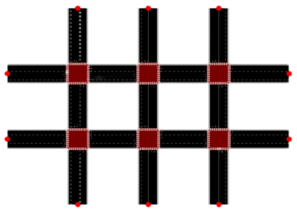
A standard grid-based network was adopted to reduce the confounding influence of irregular topology and to obtain a clear 3D-MFD pattern. The maximum speed of all roads was set to 20 m/s, each road segment was 1200 m long, and the total network length was 11.14 km. The completed simulation network is shown in Figure 2.

Signalized control was configured at each intersection. For the four-lane, six-intersection simulation network, the green phases and signal timing scheme are summarized in

Table 1. Distribution of green-light phases.

Signal Cycle	Green Light Phase Duration(s)
(s)	Phase ①	(s)	Phase ①	(s)	Phase ①	(s)
176

and

Table 2. Distribution of signal phases.

Signal Cycle	Green Light Phase Duration(s)
(s)	Phase ①	Phase ②	Phase ③	Phase ④	Phase ⑤	Phase ⑥
176	0–37	42–58	63–75	82–110	115–155	160–176

.

3.1.2. Public Transport Infrastructure Settings

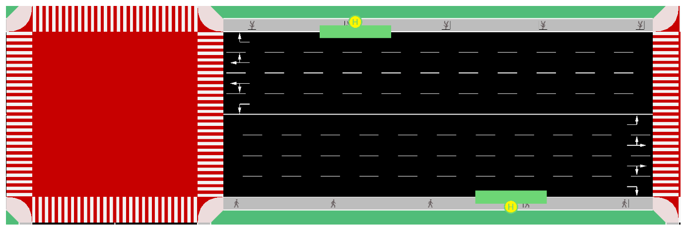
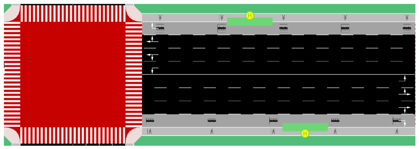
Figure 3 shows the bus-stop layout, and Figure 4 shows the dedicated bus-lane configuration. The simulation network contains 34 road segments and 34 bus stops. To reduce interference with through traffic and to facilitate boarding and alighting, bus stops were placed between the rightmost lane and the sidewalk.

3.1.3. Traffic Demand Configuration

A total of 60 OD demand pairs were configured, including 10 bus demand pairs and 50 private-vehicle demand pairs. The total number of vehicles loaded into the network during the simulation period was fixed at 15,000, and the mode-specific input volumes were determined by the experimental scenarios.

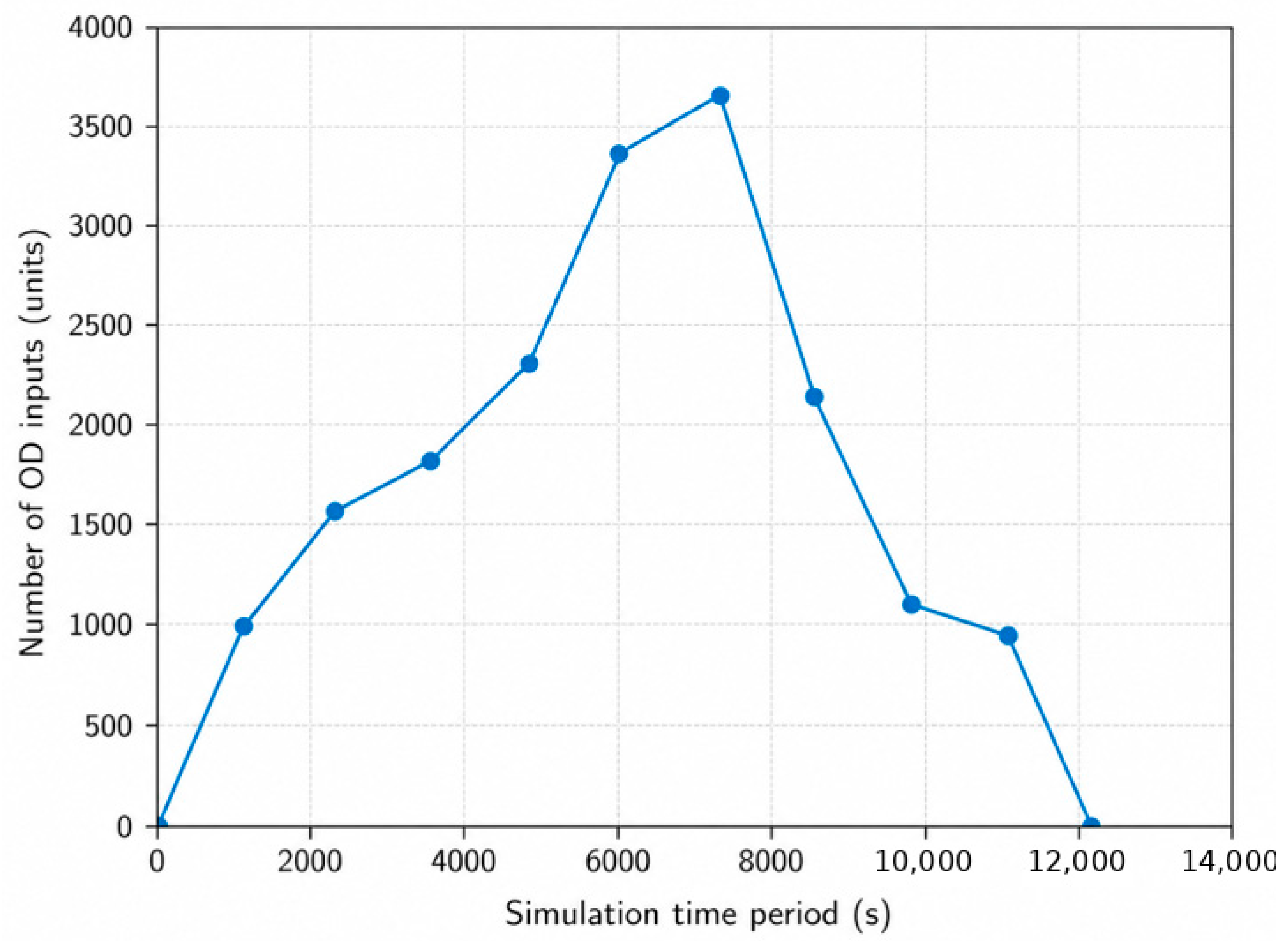
The demand profile is shown in Figure 5. Before the peak period, vehicles entered the network at a low rate. After 2000 s, the input rate increased to represent the onset of peak-hour traffic. Demand reached its maximum between 6000 and 8000 s and then gradually decreased until vehicle input stopped at 12,000 s.

To construct the 3D-MFD, three variables are required for each aggregation interval: private-vehicle accumulation, bus accumulation, and total network flow. Because SUMO does not directly output network accumulation in the required 3D-MFD form, link-level density, length, occupancy, speed, and flow-related indicators were aggregated to obtain the network-level variables.

Table 3. Representative SUMO simulation output.

Simulation Start	Simulation End	Average Vehicle Density	Road Name	Single-Lane Density	Road Segment Occupancy (%)	Average Vehicle Speed (m/s)	Ratio of Average Vehicle Speed to Maximum Speed (%)
0	300	5.61	A1B1	1.12	0.63	7.06	0.51
0	300	6.56	A2B2	1.31	0.85	6.91	0.5
0	300	5.49	B0B1	1.1	0.7	7.31	0.53
0	300	0.86	B1A1	0.17	0.12	11.07	0.8
0	300	1.62	B1B0	0.32	0.16	12.53	0.9
0	300	4.37	B1B2	0.87	0.43	8.53	0.61

presents representative SUMO outputs.

After extracting the link-level indicators, the accumulation of each mode was calculated by summing density multiplied by link length over all links, and network flow was calculated by aggregating link flows within each time interval. Vehicle units were converted to passenger-car units (pcu) when required; a bus conversion factor of 1.3 was adopted according to the Public Transport Metropolis Assessment and Evaluation Index System of the Ministry of Transport of China.

The main simulation assumptions were as follows. First, demand was exogenously loaded and route choice was kept consistent across comparable scenarios so that differences in the response variable could be attributed mainly to the tested factors. Second, fixed-time signal plans were used to avoid confounding the factor effects with adaptive signal control. Third, buses and private vehicles followed SUMO’s microscopic car-following and lane-changing logic with scenario-specific lane-changing willingness coefficients. Fourth, passenger boarding and alighting were represented through dwell-time intervals rather than through an explicit stop-level passenger-arrival model. These assumptions improve experimental controllability, but they also delimit the real-world interpretation of the results.

Table 4. Partial bus simulation output under the test scenario.

Statistics Start	Statistics End	Cumulative Road Network Traffic Volume (pcu)	Cumulative Road Network Flow Rate (pcu/h)
0	300	52	897
300	600	161	2646
600	900	176	2992
900	1200	176	2975
1200	1500	178	2945
1500	1800	177	3040

and

Table 5. Partial private-vehicle simulation output under the test scenario.

Statistics Start	Statistics End	Cumulative Road Network Traffic Volume (pcu)	Cumulative Road Network Flow Rate (pcu/h)
0	300	167	4115
300	600	269	6367
600	900	394	9480
900	1200	408	9860
1200	1500	428	10,247
1500	1800	509	12,528

show representative outputs for buses and private vehicles, respectively. Using the same aggregation procedure, the network-level bus accumulation, private-vehicle accumulation, and total flow were obtained for each time interval and used as the input data for 3D-MFD fitting.

3.2. 3D-MFD Estimation and Capacity Acquisition

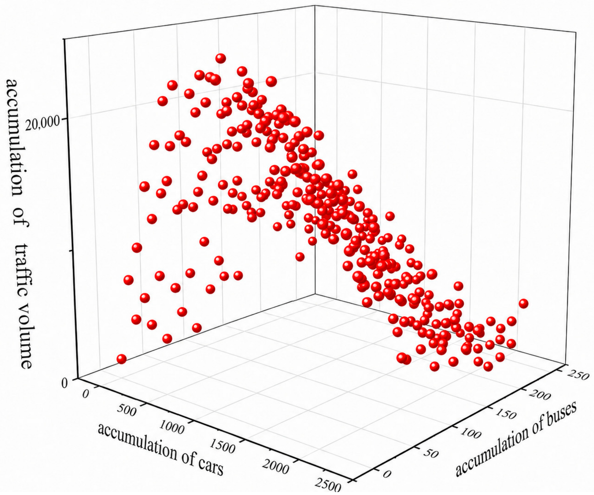
The simulated observations were used to plot the 3D-MFD scatter diagram shown in Figure 6. Network flow initially increases with the accumulation of both modes. After the accumulation reaches a critical region, however, further loading does not increase flow and may reduce it, indicating the transition from efficient operation to oversaturation.

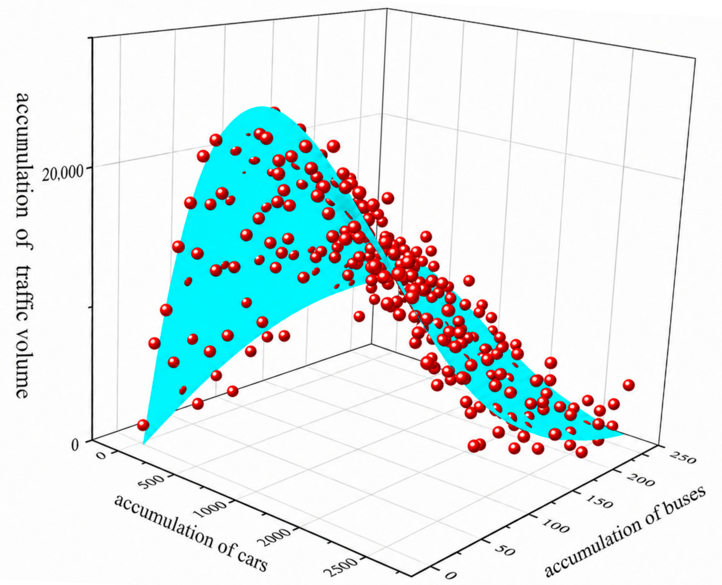
A nonlinear surface-fitting procedure was then applied to estimate the analytical 3D-MFD function. The fitted parameters were obtained after seven Levenberg–Marquardt iterations, and the resulting surface is shown in Figure 7. The coefficient of determination was $R^2=0.9357$, indicating that the fitted surface captures the main macroscopic trend in the simulated data.

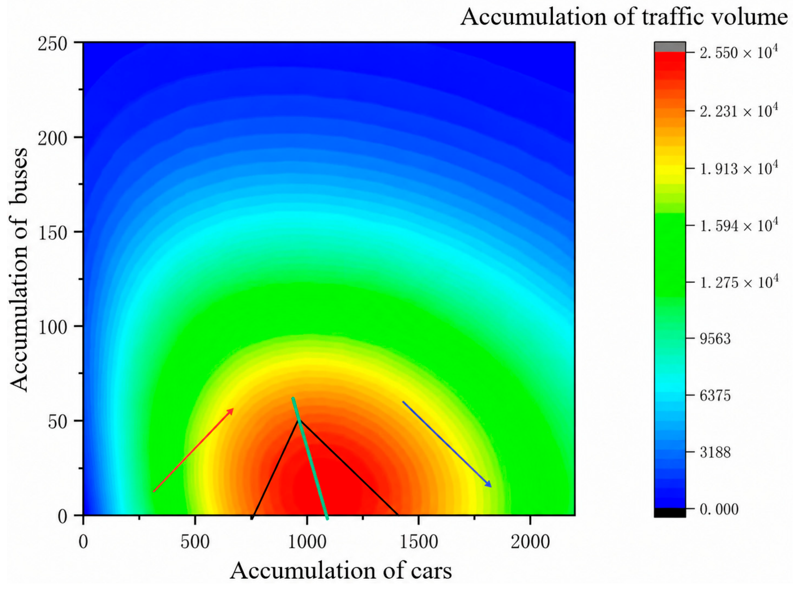
Figure 8 presents the two-dimensional projection of the fitted 3D-MFD. The projection identifies the high-performance region of the bimodal network. In the base test scenario, the bus accumulation is approximately 50 pcu, the private-vehicle accumulation is approximately 1226 pcu, and the corresponding network capacity is 23,578 pcu/h. This value is treated as the capacity estimate for the illustrative base scenario, whereas the orthogonal experiments in Section 3.4 are used to screen factor-level combinations more systematically.

3.3. Key Factors Affecting Capacity Under Bimodal Conditions

To identify improvement paths, multi-factor and multi-level scenarios were established using orthogonal experimental design. For each scenario, network capacity was extracted from the 3D-MFD-based procedure. Range analysis and ANOVA were then used to rank factor importance and test statistical significance.

Based on previous studies of MFDs, bus priority, multimodal network performance, and simulation-based bus-lane design [22,23,24,25,26,27,28,31,32], four factors were selected: the proportion of dedicated bus lanes to total network length, average bus dwell time, the bus-to-private-vehicle ratio, and driver lane-changing willingness. These factors were chosen because they correspond to four planning or operational levers that cities can observe or regulate: road-space allocation, bus-stop service process, modal composition/fleet intensity, and mixed-traffic interaction. They also represent different decision time scales, from infrastructure design to daily dispatching and behavioral response.

Four levels were specified for each factor to cover a realistic but controllable range. The dedicated bus-lane proportion was set to 0%, 4%, 8%, and 12%, using the observed proportion in Beijing (11.6%) as an upper reference while allowing comparison with a no-bus-lane baseline. Bus dwell time was divided into 6–9 s, 9–12 s, 12–15 s, and 15–20 s based on measured values ranging from 4 to 60.2 s with an average of 12.9 s, so the selected intervals represent short, medium, and relatively delayed stop operations. The bus-to-private-vehicle ratio was set to 5%, 7%, 9%, and 11% to represent increasing public-transport vehicle presence under peak traffic loading. Lane-changing willingness was represented by coefficients of 0.2, 0.4, 0.6, and 0.8, covering conservative to aggressive merging behavior in SUMO.

Because the experiment includes four factors and four levels, a 16-run orthogonal table was selected.

Table 6. Orthogonal experimental design.

Test Scenario	Proportion of Dedicated Bus Lanes to Total Road Length	Average Bus Dwell Time	Driver Lane-Changing Willingness	Ratio of Number of Buses to Number of Social Vehicles
1	0%	9–12 s	0.6	11%
2	4%	9–12 s	0.8	9%
3	4%	12–15 s	0.6	5%
4	12%	9–12 s	0.4	5%
5	8%	15–20 s	0.8	5%
6	8%	9–12 s	0.2	7%
7	0%	6–9 s	0.2	5%
8	0%	12–15 s	0.8	7%
9	12%	15–20 s	0.6	7%
10	0%	15–20 s	0.4	9%
11	4%	6–9 s	0.4	7%
12	12%	12–15 s	0.2	9%
13	12%	6–9 s	0.8	11%
14	8%	12–15 s	0.4	11%
15	8%	6–9 s	0.6	9%
16	4%	15–20 s	0.2	11%

lists the final scenario design.

The 16 scenarios were simulated independently. The extracted capacity value for each scenario served as the response variable for the subsequent range analysis and ANOVA.

3.4. Orthogonal Experimental Results

Table 7. Orthogonal experimental scenarios and capacity results.

Test Scenario	Ratio of Dedicated Bus Lanes to Total Road Length	Average Bus Dwell Time	Driver Lane-Changing Willingness	Ratio of Number of Buses to Number of Social Vehicles	Road Network Traffic Capacity (pcu/h)
1	0%	9–12 s	0.6	11%	21,538
2	4%	9–12 s	0.8	9%	23,578
3	4%	12–15 s	0.6	5%	26,173
4	12%	9–12 s	0.4	5%	20,882
5	8%	15–20 s	0.8	5%	22,140
6	8%	9–12 s	0.2	7%	23,094
7	0%	6–9 s	0.2	5%	24,255
8	0%	12–15 s	0.8	7%	23,011
9	12%	15–20 s	0.6	7%	22,777
10	0%	15–20 s	0.4	9%	21,091
11	4%	6–9 s	0.4	7%	26,733
12	12%	12–15 s	0.2	9%	22,030
13	12%	6–9 s	0.8	11%	20,209
14	8%	12–15 s	0.4	11%	20,823
15	8%	6–9 s	0.6	9%	22,181
16	4%	15–20 s	0.2	11%	23,854

summarizes the 16 orthogonal scenarios and their estimated capacity values. The highest observed capacity is 26,733 pcu/h in Scenario 11, corresponding to a 4% bus-lane proportion, a 6–9 s bus dwell time, a lane-changing willingness coefficient of 0.4, and a 7% bus-to-private-vehicle ratio.

3.4.1. Range Analysis

The range-analysis results are shown in

Table 8. Range-analysis results.

Item	Level	Ratio of Dedicated Bus Lanes to Total Road Length	Average Bus Dwell Time	Driver Lane- Changing Willingness	Ratio of Number of Buses to Number of Social Vehicles
K	1	89,895	93,378	93,233	93,450
	2	100,338	89,092	89,529	95,615
	3	88,238	92,037	92,669	88,880
	4	85,898	89,862	88,938	86,424
K avg	1	22,473.75	23,344.5	23,308.25	23,362.5
	2	25,084.5	22,273	22,382.25	23,903.75
	3	22,059.5	23,009.25	23,167.25	22,220
	4	21,474.5	22,465.5	22,234.5	21,606
$R$		3610	1071.5	1073.75	2297.75

. The factors are ranked by their range values as follows: dedicated bus-lane proportion ($R=3610$), bus-to-private-vehicle ratio ($R=2297.75$), driver lane-changing willingness ($R=1073.5$), and average bus dwell time ($R=1071.5$). Thus, road-space allocation and modal composition are the two most influential factors in the simulated bimodal network.

3.4.2. Analysis of Variance

ANOVA was conducted to test the statistical significance of the four factors. As shown in

Table 9. ANOVA results.

	Sum of Squares	df	Mean Square	F	p
Ratio of Dedicated Bus Lanes to Total Road Length	30,511,069.19	3	10,170,356.4	34.219	0.008 **
Average Bus Dwell Time	2,907,930.187	3	969,310.062	3.261	0.179
Driver Lane-Changing Willingness	3,538,373.688	3	1,179,457.896	3.968	0.144
Ratio of Number of Buses to Number of Social Vehicles	13,175,215.19	3	4,391,738.396	14.776	0.027 *
Residual	891,650.688	3	297,216.896
$R^2=0.983$

Note: * $p<0.05$; ** $p<0.01$.

, dedicated bus-lane proportion is highly significant ($p=0.008$), and the bus-to-private-vehicle ratio is significant ($p=0.027$). Average bus dwell time and lane-changing willingness are not significant at the 0.05 level in this experiment. These results are consistent with the range-analysis ranking.

3.5. Capacity-Improvement Strategies

3.5.1. Capacity Distribution Under Key Factor Levels

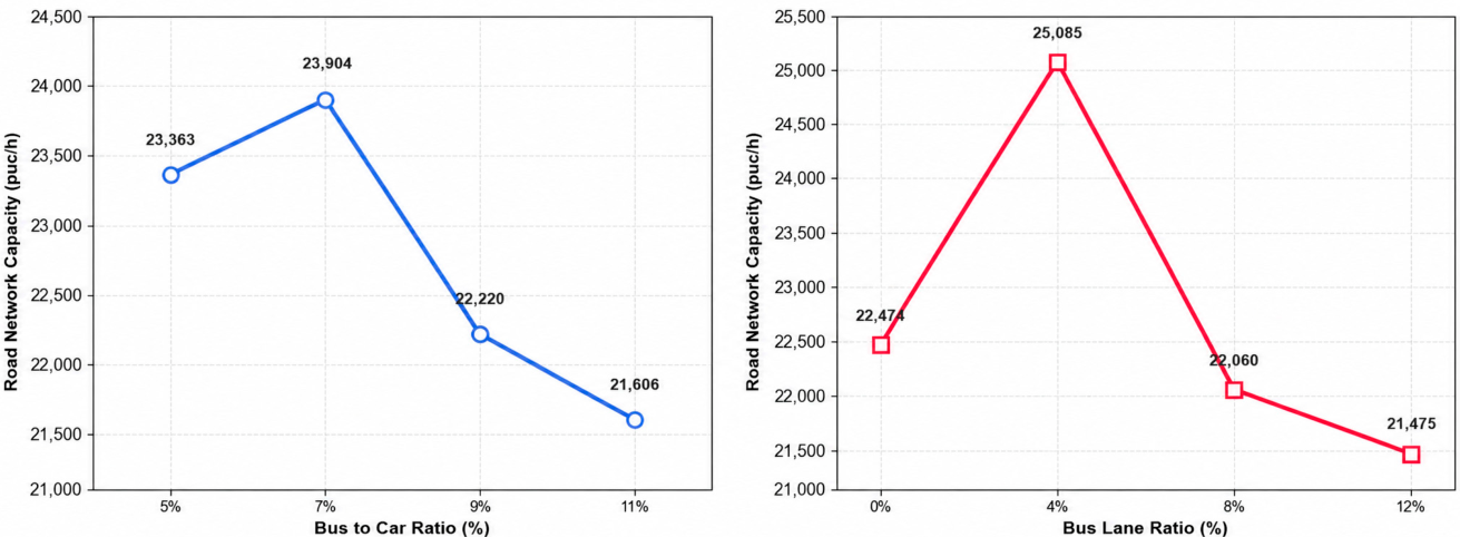
The bus-to-social-vehicle ratio showed a rise-and-fall relationship with capacity, as shown in Figure 9. At 5%, the bus share was relatively low and the road network still had unused potential for public transport service. At 7%, capacity reached a favorable balance between bus service and social-vehicle operation. When the ratio increased to 9% or 11%, buses occupied more operational space and intensified interactions with social vehicles, reducing total capacity.

The dedicated bus-lane proportion shows a similar nonlinear pattern. Without dedicated bus lanes, buses and private vehicles share the same road space, and bus stops and lower bus speeds interfere with private-vehicle movement. A moderate bus-lane provision separates traffic streams and improves efficiency. However, excessive bus-lane length reduces the road space available to private vehicles and therefore lowers total network capacity.

Accordingly, the simulation results support a moderate bus-priority strategy rather than an unrestricted expansion of bus lanes. The recommended levels are a 4% bus-lane share and a 7% bus-to-private-vehicle ratio under the assumptions of this grid network and demand setting.

3.5.2. Strategy Implications

The dominant effect of bus-lane proportion indicates that spatial allocation is the primary lever for improving capacity in the simulated network. A limited but well-targeted bus-lane system can reduce bus–private-vehicle interference, but excessive allocation to buses may reduce the capacity available to general traffic. Therefore, bus lanes should be deployed preferentially on corridors where high bus demand and severe mixed-traffic conflicts coexist.

The bus-to-private-vehicle ratio should also be managed as an operational indicator. Too few buses may cause long passenger waiting times and underutilization of public-transport priority, whereas too many buses may increase interference and occupy excessive road resources. The 7% level should be interpreted as a scenario-specific reference rather than a universal prescription.

Overall, the optimal strategy identified by the orthogonal experiment is to maintain a 4% bus-lane proportion and a 7% bus-to-private-vehicle ratio. This combination balances bus-priority benefits with the need to preserve general traffic capacity in the simulated bimodal network.

In planning terms, the magnitude of the factor effects implies that geometric and modal-composition measures should receive priority over fine behavioral parameters when a city first screens bus-priority strategies. In this experiment, changing the bus-lane proportion or the bus-to-private-vehicle ratio altered the capacity response by several thousand pcu/h, whereas dwell time and lane-changing willingness produced smaller and statistically insignificant differences. Therefore, the recommended 4% and 7% values should be read as a starting point for local scenario testing: similar performance is most likely in dense urban subnetworks with comparable bus-stop density, moderate bus-priority coverage, fixed-time signals, and peak-period mixed traffic demand.

The scenario-level results further support this interpretation. The highest-capacity scenario combined a moderate 4% bus-lane proportion, a 7% bus-to-private-vehicle ratio, a short 6–9 s dwell-time interval, and moderate lane-changing willingness. This combination can be interpreted as balancing bus-priority benefits with the preservation of general-purpose traffic capacity: bus operations receive enough reserved space to reduce mixed-traffic interference, while the remaining road space is still sufficient to prevent severe spillover congestion in private-vehicle lanes. By contrast, larger bus-lane shares or higher bus-to-private-vehicle ratios are expected to shift congestion toward general-purpose lanes or intensify interactions near bus stops and intersections, thereby reducing the vehicle-based capacity response.

3.6. Simulation-Based Transferability Assessment on a Real-World Network

The selected subnetwork is located in southeast Chaoyang District, Beijing, an urban area with intensive commuting, commercial, residential, and public-transport activities. The study area is bounded approximately by Baiziwan Road to the north, Guangqu Road to the south, Xidawang Road to the west, and East Fourth Ring Middle Road to the east. Compared with the idealized grid used in the main experiment, this subnetwork contains a more heterogeneous urban road structure, including arterial roads, ring-road access links, collector roads, and local streets. It was selected because buses and private vehicles operate in close spatial interaction within the area, and several corridors contain bus-priority facilities, making the subnetwork suitable for examining whether the parameter combination derived from the grid network remains reasonable under a real-city road topology.

To reduce the risk that the strategy derived from the idealized grid network is a topology-specific artifact, a simulation-based transferability assessment was conducted on this Beijing subnetwork. The assessment used the real road layout as the simulation topology, but the evidence remains simulation-based rather than field-observed validation. The simulated subnetwork includes Jiulongshan North Road, Maoxing Road, Xidawang Road, Baiziwan Road, East Fourth Ring Middle Road, Guangqu Road, and Songyu South Road. Among these links, Guangqu Road, Xidawang Road, and Songyu South Road contain bus-priority facilities. The selected road segments have a total length of approximately 13.5 km, include 21 bus stops, and are served by 11 bus routes. Road-segment lengths, channelization, cross-section forms, bus-lane layouts, and bus-stop locations were collected from field inspections, OpenStreetMap road geometry [33], and digital map interpretation.

Because the orthogonal analysis identified bus-lane proportion and the bus-to-private-vehicle ratio as the two statistically significant factors, the transferability assessment varied only these two parameters while keeping the remaining simulation assumptions consistent within the Beijing subnetwork. Sixteen assessment scenarios were configured, as summarized in

Table 10. Transferability-assessment scenarios and capacity estimates for the Beijing subnetwork.

Capacity (pcu/h)	Bus-To-Private-Vehicle Ratio	Bus-Lane Proportion	Scenario
21,547	11%	2%	1
24,113	9%	4%	2
24,156	5%	4%	3
26,784	5%	12%	4
26,451	5%	8%	5
24,332	7%	8%	6
25,471	5%	2%	7
26,784	7%	2%	8
23,220	7%	12%	9
23,215	9%	2%	10
27,548	7%	4%	11
21,545	9%	12%	12
20,334	11%	12%	13
21,049	11%	8%	14
22,110	9%	8%	15
22,485	11%	4%	16

. The tested bus-lane proportions were 2%, 4%, 8%, and 12%, while the tested bus-to-private-vehicle ratios were 5%, 7%, 9%, and 11%.

The assessment results indicate that Scenario 11, with a 4% bus-lane proportion and a 7% bus-to-private-vehicle ratio, produced the highest capacity among the 16 tested Beijing subnetwork scenarios (27,548 pcu/h). This value is 2.85% higher than the next-best assessed capacity of 26,784 pcu/h and 15.64% higher than the mean assessed capacity of 23,821.5 pcu/h. Thus, the second simulated topology yields the same highest-capacity parameter combination as the grid-network experiment. This agreement provides preliminary support for the parameter combination within the simulated experimental scope, but it should not be interpreted as empirical proof of universal effectiveness.

The results should therefore be interpreted as a topology-transfer simulation check rather than direct field validation. They strengthen the internal consistency and transferability plausibility of the proposed strategy by applying it to a more heterogeneous road layout, but the values of 4% and 7% remain scenario-specific and require calibration with observed traffic, bus GPS/AVL, and detector data before broader application.

4. Discussion

This section interprets the results in relation to the research objectives, the existing literature, practical application, and the additional transferability assessment, while also clarifying the limitations of the simulation-based evidence.

4.1. Alignment with the Research Objectives

The first objective was achieved by constructing a controllable SUMO-based bimodal network and extracting the variables required for 3D-MFD estimation. The fitted surface achieved $R^2=0.9357$, which indicates that the model captures the major trend of the simulated macroscopic relationship. Nevertheless, R² should be interpreted as a goodness-of-fit measure for the stylized simulation data rather than as proof of universal validity.

The second objective was achieved through the 16-scenario orthogonal experiment. Range analysis and ANOVA consistently identify bus-lane proportion and bus-to-private-vehicle ratio as the two dominant factors. This result supports the hypothesis that spatial priority and modal composition jointly determine capacity in bimodal networks.

The third objective was addressed by deriving a practical parameter combination and then examining it under a second simulated topology. In the grid experiment, the results suggest that a 4% bus-lane proportion and a 7% bus-to-private-vehicle ratio provide the most favorable capacity response, with the best observed scenario reaching 26,733 pcu/h. The Beijing subnetwork assessment identified the same two-factor combination as the highest-capacity tested scenario, reaching 27,548 pcu/h. This result supports the internal consistency of the simulation findings but does not establish a universal design optimum.

4.2. Comparison with Existing Literature

Compared with the original 3D-MFD formulation for mixed bimodal networks [20], this study emphasizes capacity extraction and parameter screening rather than only describing the existence and shape of the 3D-MFD.

The finding that moderate road-space allocation improves performance is consistent with multimodal MFD studies showing that bus priority and modal composition affect network efficiency [22,23,24,25,26,27,28]. The additional contribution of this paper is to provide a transparent orthogonal simulation design that translates these effects into candidate parameter levels for a specific network configuration.

Compared with dynamic capacity estimation based on conventional MFDs [11], the proposed framework explicitly retains the distinction between bus accumulation and private-vehicle accumulation. This distinction is important when capacity management must also preserve public-transport service levels.

4.3. Practical Implications

For traffic planners, the results suggest that bus-priority infrastructure should be designed as a balanced network-level resource rather than as a simple expansion target. A moderate bus-lane share can reduce bus–private-vehicle interference and improve network performance, but excessive bus-lane allocation can shift congestion to private-vehicle lanes and reduce the total vehicle-based capacity. The practical planning implication is that bus lanes should be prioritized on corridors where bus demand, stop density, and mixed-traffic conflicts are high, while parallel general-purpose capacity and signal progression should be checked before network-wide expansion.

The results are expected to be most transferable to urban subnetworks with dense surface bus services, limited possibilities for road widening, and demand levels close to the onset of oversaturation. In cities with very high bus occupancy, stronger public-transport policy goals, or severe environmental constraints, the preferred solution may intentionally sacrifice some vehicle-based flow to improve person throughput and emissions performance. Therefore, the proposed workflow should be used to support locally calibrated decision-making rather than to impose a single bus-lane or fleet-share standard. More specifically, the workflow is most suitable for central or inner-urban subnetworks similar to the Beijing case, where arterial roads, collector roads, local streets, dense bus stops, and bus-service corridors coexist under peak-period mixed traffic demand.

For Applied Sciences readers, the methodological value of the study lies in the reproducible workflow: simulate controlled bimodal scenarios, extract 3D-MFD variables, estimate capacity, and statistically screen policy parameters. This workflow can be transferred to other networks once local OD demand, bus operations, and signal settings are calibrated.

4.4. Limitations

This study has four main limitations. First, the main mechanism analysis is based on an idealized grid network. Although a Beijing subnetwork was added for transferability assessment, real road networks may still contain heterogeneous road grades, irregular intersections, one-way streets, parking disturbances, freight loading, non-motorized traffic, and uneven bus-stop spacing, all of which may affect the 3D-MFD shape and the optimal parameter levels. In such networks, a less regular topology may weaken the smoothness of the 3D-MFD surface, make capacity more sensitive to local bottlenecks, and shift the optimal bus-priority level away from the value observed in the grid experiment.

Second, fixed-time signal control and a single temporal demand pattern were adopted. In practice, coordinated signal timing, transit signal priority, offset plans, incident conditions, and morning-evening directional imbalance may change both the location of the critical accumulation and the observed capacity response. For example, coordinated signal timing or transit signal priority may improve bus progression and shift the critical accumulation, whereas incident conditions or strong directional imbalance may lower the observed capacity and change the best-performing factor combination.

Third, real-world driver behavior was represented through a limited lane-changing willingness parameter. Actual behavior may vary with enforcement of bus lanes, curbside parking, familiarity with the network, weather, vehicle automation, and compliance with lane-use restrictions. These factors may alter bus–private-vehicle interactions near stops and intersections. More aggressive lane-changing, weak compliance with bus-lane restrictions, or frequent curbside disturbances would likely intensify bus–private-vehicle interactions near stops and intersections and may reduce the effectiveness of the recommended bus-priority settings.

Fourth, both the grid experiment and the Beijing subnetwork assessment are simulation-based. Therefore, the reported 4% and 7% values should be treated as scenario-specific findings rather than universal design standards. Future work should calibrate and validate the framework with empirical OD, trajectory, loop-detector, signal-timing, bus AVL, and passenger-count data and test whether the same factor ranking holds in heterogeneous urban networks.

5. Conclusions

This paper proposed a 3D-MFD-based framework for assessing road network capacity and identifying improvement strategies in a bimodal urban traffic network. The framework integrates SUMO simulation, 3D-MFD surface fitting, orthogonal experimental design, range analysis, ANOVA, and a supplementary simulation-based transferability assessment.

The base 3D-MFD fitting produced $R^2=0.9357$ and an illustrative capacity estimate of 23,578 pcu/h. Across the 16 orthogonal grid-network scenarios, the highest observed capacity was 26,733 pcu/h. The statistical results indicate that dedicated bus-lane proportion and bus-to-private-vehicle ratio are the dominant capacity-influencing factors, whereas bus dwell time and lane-changing willingness are less significant in the tested design.

Under the assumptions of the tested networks, demand profile, and parameter levels used in this study, the recommended strategy is to set the bus-lane proportion to 4% of the total network length and the bus-to-private-vehicle ratio to 7%. The Beijing subnetwork assessment produced the highest tested capacity under the same combination, which supports the robustness of the strategy within the simulated experimental scope but does not establish a universal optimum.

Future research should further validate the proposed framework using calibrated empirical OD demand, trajectory, loop-detector, signal-timing, bus AVL, and passenger-count data, and should examine dynamic control strategies under changing demand conditions. Further work should also incorporate passenger-oriented and emissions indicators so that the vehicle-based 3D-MFD can be linked more directly to social optimization, person-based mobility performance, and environmental sustainability.

References

- Chen, H. Research on Prevention, Control and Restoration Strategies of Urban Road Network Traffic Congestion Oriented to Service Resilience. Ph.D. Thesis, Chang’an University, Xi’an, China, 2023. [Google Scholar]
- Jiang, K.; Sun, H.; Wang, Y. Application of Connected and Autonomous Vehicles in Urban Traffic Congestion. Agric. Mach. Use Maint. 2025, 5, 122–124. [Google Scholar]
- Hao, W.; Xiao, L.; Zhang, Z.; Zheng, N. Reliability Analysis of Urban Road Network Capacity under Connected and Autonomous Environment. J. Traffic Inf. Saf. 2022, 40, 44–52. [Google Scholar]
- Liu, X. Impact of Dynamic Bus Priority Lanes on Equivalent Traffic Capacity and Its Setting Method. Master’s Thesis, Northeast Forestry University, Harbin, China, 2024. [Google Scholar]
- Zhou, Y. Research on Improving Operational Efficiency of Bus Lanes Based on Mixed Traffic Flow. Master’s Thesis, Chongqing Jiaotong University, Chongqing, China, 2021. [Google Scholar]
- Loder, A.; Bliemer, M.C.J.; Axhausen, K.W. Optimal Pricing and Investment in a Multi-Modal City-Introducing a Macroscopic Network Design Problem Based on the MFD. Transp. Res. Part A Policy Pract. 2022, 156, 113–132. [Google Scholar] [CrossRef]
- Mansourianfar, M.H.; Gu, Z.; Saberi, M. Joint Routing and Pricing Control in Bimodal Mixed Autonomy Networks with Elastic Demand and Three-Dimensional Passenger Macroscopic Fundamental Diagram. Transp. Res. Rec. 2024, 2678, 1250–1264. [Google Scholar] [CrossRef]
- Shao, C.; Pang, J.; Lu, K.; Li, X. Road Network Capacity Based on Spatiotemporal Consumption Method and Operational Efficiency. J. Beijing Univ. Technol. 2019, 45, 895–903. [Google Scholar]
- Jin, C. Parameter Calibration of Microscopic Traffic Simulation Model and Research on Road Network Capacity and Its Reliability. Ph.D. Thesis, Kunming University of Science and Technology, Kunming, China, 2013. [Google Scholar]
- Guo, L.; Yin, H.; Zhang, J. A Penalized Sequential Convex Programming Approach for Continuous Network Design Problems. Inf. J. Comput. 2025, 38, 490–506. [Google Scholar] [CrossRef]
- Hong, R. Research on Urban Road Network Traffic Capacity Estimation and Operational State Discrimination Method Based on Multi-Source Data. Ph.D. Thesis, Southeast University, Nanjing, China, 2021. [Google Scholar]
- Liao, D.; Ma, W. A Literature Review on Network Traffic Flow Macroscopic Fundamental Diagram. In Proceedings of the 7th China Intelligent Transportation Annual Conference, Shanghai, China, 26–28 September 2012; pp. 4–9. [Google Scholar]
- Mazloumian, A.; Geroliminis, N.; Helbing, D. The Spatial Variability of Vehicle Densities as Determinant of Urban Network Capacity. Philos. Trans. R. Soc. A Math. Phys. Eng. Sci. 2010, 368, 4627–4647. [Google Scholar] [CrossRef] [PubMed]
- Geroliminis, N.; Daganzo, C.F. Existence of Urban-Scale Macroscopic Fundamental Diagrams: Some Experimental Findings. Transp. Res. Part B Methodol. 2008, 42, 759–770. [Google Scholar] [CrossRef]
- Daganzo, C.F. Urban Gridlock: Macroscopic Modeling and Mitigation Approaches. Transp. Res. Part B Methodol. 2007, 41, 49–62. [Google Scholar] [CrossRef]
- Yang, G. Research on Urban Bus Priority Technology Based on Three-Dimensional Macroscopic Fundamental Diagram. Master’s Thesis, Henan University of Science and Technology, Luoyang, China, 2023. [Google Scholar]
- Wang, P.; Li, Y.; Yang, D.; Yang, H. Traffic Signal Control Model of Macroscopic Fundamental Diagram Based on Hierarchical Control. J. Comput. Appl. 2021, 41, 571–576. [Google Scholar]
- Zhang, W.; Chen, S.; Ding, H. Feedback Valve Control Considering Traffic Congestion at Boundary Intersections. Control Theory Appl. 2019, 36, 241–248. [Google Scholar]
- Keyvan-Ekbatani, M.; Papageorgiou, M.; Papamichail, I. Urban Congestion Gating Control Based on Reduced Operational Network Fundamental Diagrams. Transp. Res. Part C Emerg. Technol. 2013, 33, 74–87. [Google Scholar] [CrossRef]
- Geroliminis, N.; Zheng, N.; Ampountolas, K. A Three-Dimensional Macroscopic Fundamental Diagram for Mixed Bi-Modal Urban Networks. Transp. Res. Part C Emerg. Technol. 2014, 42, 168–181. [Google Scholar] [CrossRef]
- Johari, M.; Keyvan-Ekbatani, M. Macroscopic Modeling of Mixed Bi-Modal Urban Networks: A Hybrid Model of Accumulation- and Trip-Based Principles. Transp. Res. Part B Methodol. 2024, 182, 102921. [Google Scholar] [CrossRef]
- Dakic, I.; Leclercq, L.; Menendez, M. On the Optimization of the Bus Network Design: An Analytical Approach Based on the Three-Dimensional Macroscopic Fundamental Diagram. Transp. Res. Part B Methodol. 2021, 149, 393–417. [Google Scholar] [CrossRef]
- Bhavathrathan, B.K.; Patil, G.R. Capacity Uncertainty on Urban Road Networks: A Critical State and Its Applicability in Resilience Quantification. Comput. Environ. Urban Syst. 2015, 54, 108–118. [Google Scholar] [CrossRef]
- Loder, A.; Dakic, I.; Bressan, L.; Ambühl, L.; Bliemer, M.C.; Menendez, M.; Axhausen, K.W. Capturing Network Properties with a Functional Form for the Multi-Modal Macroscopic Fundamental Diagram. Transp. Res. Part B Methodol. 2019, 129, 1–19. [Google Scholar] [CrossRef]
- Loder, A.; Ambuhl, L.; Menendez, M.; Axhausen, K.W. Empirics of Multi-Modal Traffic Networks: Using the 3D Macroscopic Fundamental Diagram. Transp. Res. Part C Emerg. Technol. 2017, 82, 88–101. [Google Scholar] [CrossRef]
- Boyaci, B.; Geroliminis, N. Estimation of the Network Capacity for Multimodal Urban Systems. Procedia Soc. Behav. Sci. 2011, 16, 803–813. [Google Scholar] [CrossRef]
- Dakic, I.; Yang, K.; Menendez, M.; Chow, J.Y.J. On the Design of an Optimal Flexible Bus Dispatching System with Modular Bus Units: Using the Three-Dimensional Macroscopic Fundamental Diagram. Transp. Res. Part B Methodol. 2021, 148, 38–59. [Google Scholar] [CrossRef]
- Zheng, N.; Geroliminis, N. On the Distribution of Urban Road Space for Multimodal Congested Networks. Transp. Res. Part B Methodol. 2013, 57, 326–341. [Google Scholar] [CrossRef]
- Loder, A.; Ambuhl, L.; Menendez, M.; Axhausen, K.W. Understanding Traffic Capacity of Urban Networks. Sci. Rep. 2019, 9, 16283. [Google Scholar] [CrossRef] [PubMed]
- Lopez, P.A.; Behrisch, M.; Bieker-Walz, L.; Erdmann, J.; Fletteröd, Y.-P.; Hilbrich, R.; Lücken, L.; Rummel, J.; Wagner, P.; Wießner, E. Microscopic Traffic Simulation Using SUMO. In Proceedings of the 2018 21st International Conference on Intelligent Transportation Systems (ITSC), Maui, HI, USA, 4–7 November 2018; pp. 2575–2582. [Google Scholar] [CrossRef]
- Dantsuji, T.; Fukuda, D.; Zheng, N. A Macroscopic Approach for Optimizing Road Space Allocation of Bus Lanes in Multimodal Urban Networks Through Simulation Analysis: An Application to the Tokyo CBD Network. In Proceedings of the 2017 IEEE 20th International Conference on Intelligent Transportation Systems, Yokohama, Japan, 16–19 October 2017. [Google Scholar] [CrossRef]
- Zheng, N.; Dantsuji, T.; Wang, P.; Geroliminis, N. Macroscopic Approach for Optimizing Road Space Allocation of Bus Lanes in Multimodal Urban Networks Through Simulation Analysis. Transp. Res. Rec. 2017, 2651, 42–51. [Google Scholar] [CrossRef]
- OpenStreetMap contributors. Planet Dump and Extracts. Available online: https://www.openstreetmap.org (accessed on 1 July 2026).
Figure 1.
Framework of the proposed method. The framework consists of three modules: simulation setup and data collection, 3D-MFD modeling and capacity definition, and factor analysis and strategy validation.
Figure 2.
Completed simulation road network. The red parts indicate signalized intersections, and the black line segments represent road links.
Figure 3.
Bus stop layout. Black areas indicate vehicle lanes, green areas indicate roadside pedestrian spaces or bus-stop areas, yellow symbols indicate bus-stop signs, and arrows indicate traffic directions.
Figure 4.
Dedicated bus lanes. Grey lanes indicate dedicated bus lanes, black lanes indicate general traffic lanes, green areas indicate roadside pedestrian spaces, and arrows indicate traffic directions.
Figure 5.
OD input pattern.
Figure 6.
3D-MFD scatter plot under the simulation test scenario. Red dots represent simulated traffic-state observations.
Figure 7.
Fitted 3D-MFD surface. The cyan surface represents the fitted 3D-MFD function, and the red dots represent simulated observations.
Figure 8.
Two-dimensional projection of the fitted 3D-MFD. The color gradient represents the network flow, and the arrow indicates the identified high-capacity region.
Figure 9.
Distribution of road network capacity under key factor levels.