Mode-Aware Constrained Inverse Optimization for Behind-the-Meter Energy Storage Power Estimation Under Time-of-Use Tariffs

Featured Application

This study can be applied to behind-the-meter flexible resource perception, distributed energy storage operation monitoring, demand response analysis, and distribution network scheduling. The proposed method provides a practical way to estimate behind-the-meter energy storage power using net load, photovoltaic power, and time-of-use tariff information when direct storage measurements are unavailable.

Abstract

With the increasing penetration of behind-the-meter photovoltaic generation and distributed energy storage, distribution system operators usually observe only the net load at the point of common coupling, while the actual user load and energy storage charging/discharging power are difficult to measure directly. To address this problem, this paper proposes a mode-aware constrained inverse optimization method for behind-the-meter distributed energy storage power estimation under fixed time-of-use tariffs. The proposed method uses net load, photovoltaic power, and tariff information as inputs and estimates the hidden user load, storage power, SOC trajectory, and dominant storage arbitrage mode. A mode-aware joint representation model is developed by introducing single-cycle and dual-cycle charge–discharge templates, daily action intensity factors, mode weights, and local correction terms. In addition, power limits, SOC dynamics, SOC bounds, daily energy balance constraints, tariff-response consistency, and mode selection penalty are incorporated into the inverse optimization framework to improve the physical feasibility and interpretability of the estimation results. Case studies are conducted using a 40-day hybrid dataset with a 1 h sampling interval and a 70%/30% training/testing split. The dataset is constructed from park-level user load and photovoltaic data, while the storage power profile is reconstructed according to typical time-of-use arbitrage operation. For the main dual-cycle testing case, the NRMSEs of storage power, user load, and net load are 14.75%, 3.90%, and 3.76%, respectively. The results show that the proposed method can recover the main variation trend of hidden storage power under the studied fixed time-of-use tariff scenario and provides a preliminary basis for park-level storage monitoring and flexible resource perception.

1. Introduction

With the rapid development of distributed photovoltaic generation, user-side energy storage, and flexible loads, distribution networks are changing from passive power supply systems to active systems with multiple controllable resources [1,2]. Behind-the-meter distributed energy storage can participate in peak shaving, valley filling, demand response, and time-of-use tariff arbitrage through charging and discharging. However, in practical applications, energy storage systems are usually installed behind the user meter. Therefore, distribution system operators can generally observe only the net load at the point of common coupling, while the actual user load and the charging/discharging power of the energy storage system are difficult to obtain directly.

The lack of direct measurements of behind-the-meter energy storage power brings challenges to flexible resource perception and distribution network operation. On the one hand, user load, photovoltaic generation, and energy storage power are coupled in the measured net load. On the other hand, energy storage power has bidirectional characteristics, including charging, discharging, and frequent power switching. Therefore, behind-the-meter storage power cannot be simply regarded as a conventional load component. If the storage power cannot be accurately estimated, it will be difficult for system operators to evaluate demand response capability, analyze user-side flexibility, and support subsequent optimal scheduling.

Existing non-intrusive load monitoring and data-driven disaggregation methods [3,4,5,6,7,8] provide useful ideas for recovering internal components from aggregate measurements. However, most conventional NILM methods are designed for household appliances or conventional electrical equipment with relatively clear on/off states. Behind-the-meter energy storage is different from these loads because its charging and discharging power is bidirectional and strongly affected by time-of-use tariffs, energy management strategies, power limits, and SOC constraints [9,10,11,12]. Purely data-driven methods, such as supervised regression models, can learn nonlinear relationships from historical data, but they usually require labeled storage power data during training. In practical park-level applications, directly measured behind-the-meter storage power is often unavailable. Moreover, purely data-driven estimates do not necessarily satisfy physical constraints such as charging/discharging power limits, SOC continuity, SOC bounds, and daily energy balance.

Some recent studies have investigated behind-the-meter component identification, distributed energy resource inference, virtual-battery-based flexibility modeling, and inverse optimization for price-responsive loads. These methods are useful for general BTM resource identification or aggregate flexibility representation. However, many of them aim to decompose the total load into multiple components, such as storage-like load, photovoltaic generation, thermostatically controlled load, and periodic load, or to represent price-responsive resources using virtual battery surrogate models. In contrast, they do not explicitly focus on the specific scenario where photovoltaic power is already measured while the behind-the-meter storage power remains hidden in the net load. They also do not directly distinguish the practical daily arbitrage patterns of user-side storage, such as single-cycle and dual-cycle charge–discharge behaviors under fixed time-of-use tariffs.

Different from general BTM component identification methods, this paper focuses on a more specific park-level scenario in which photovoltaic power is measured, while user load and behind-the-meter storage power are coupled in the observed net load. In this case, the key problem is not to identify all possible BTM resource components, but to estimate the hidden storage power and its operation behavior under the known time-of-use tariff structure. To address this problem, this paper introduces a mode-aware storage representation into a constrained inverse optimization framework [13,14,15]. The storage power is described using single-cycle and dual-cycle charge–discharge templates, daily action intensity factors, mode weights, and local correction terms. The single-cycle mode corresponds to the basic valley-charging and peak-discharging arbitrage strategy, while the dual-cycle mode represents multiple charging and discharging actions under multiple valley, peak, or critical peak tariff periods.

It should be noted that the proposed method is developed under specific assumptions. First, the photovoltaic power is assumed to be available as an input measurement. Second, the time-of-use tariff structure is known [16]. Third, the behind-the-meter storage system is assumed to mainly follow typical tariff-driven arbitrage behaviors in the studied case. Under these assumptions, the proposed method uses load templates, storage mode templates, tariff-response consistency, SOC dynamics, power limits, and daily energy balance constraints to reduce the non-uniqueness of the hidden component estimation problem and obtain physically feasible storage power estimates [17].

The main contributions of this paper are summarized as follows:

(1)

A constrained inverse optimization framework is proposed for behind-the-meter storage power estimation under known photovoltaic measurements and fixed time-of-use tariffs. Different from general BTM component identification methods, the proposed method focuses on estimating hidden storage power and user load from measured net load, measured photovoltaic power, and tariff information under incomplete measurement conditions.

(2)

A mode-aware storage representation is developed by constructing a storage arbitrage mode library with single-cycle and dual-cycle charge–discharge templates. The introduced mode weights provide an interpretable indicator of the dominant daily arbitrage mode, which enables the model to distinguish typical storage operation behaviors under the studied fixed tariff structure.

(3)

Operational constraints and regularization terms are incorporated into the inverse optimization model, including storage power limits, SOC dynamics, SOC bounds, daily energy balance, tariff-response consistency, mode selection penalty, and simultaneous charge–discharge suppression. These constraints reduce physically unreasonable solutions and improve the interpretability of the estimated storage power and SOC trajectory.

2. Methods

2.1. Problem Formulation

A user-side park system with distributed photovoltaic generation and behind-the-meter distributed energy storage is considered in this study [9,10,11,12]. In practical operation, the distribution system operator can usually obtain the net load power at the point of common coupling, the photovoltaic power, and the time-of-use tariff information. However, the actual user load and the charging/discharging power of the behind-the-meter energy storage system are generally not directly measured. Therefore, the main task of this study is to estimate the unobservable user load, behind-the-meter storage power, SOC trajectory, and dominant storage operation mode using limited external measurement information.

For a consistent notation, d = 1, 2, …, D denotes the day index, and h = 1, 2, …, H denotes the intra-day time interval index. The absolute time index can be written as t = (d, h). The sampling interval is denoted by Delta t. In this paper, power variables are expressed in kW, energy variables are expressed in kWh or MWh, and SOC is dimensionless.

Let $P_{\mathrm{grid}}(d,h)$ denote the net load power measured at the grid connection point, $P_{\mathrm{load}}(d,h)$ denote the actual user load power, $P_{\mathrm{PV}}(d,h)$ denote the photovoltaic output power, and $P_{\mathrm{ES}}(d,h)$ denote the behind-the-meter energy storage power. In this paper, positive $P_{\mathrm{ES}}(d,h)$ represents discharging, while negative $P_{\mathrm{ES}}(d,h)$ represents charging. When line losses are ignored, the power balance relationship among these variables can be expressed as:

$$P_{\mathrm{grid}}(d,h)=P_{\mathrm{load}}(d,h)-P_{\mathrm{PV}}(d,h)-P_{\mathrm{ES}}(d,h),$$

(1)

In the above equation, $P_{\mathrm{grid}}(d,h)$, $P_{\mathrm{PV}}(d,h)$, and the time-of-use tariff π($d,h$) are known variables, while $P_{\mathrm{load}}(d,h)$ and $P_{\mathrm{ES}}(d,h)$ are unknown variables to be estimated. Equation (1) describes the coupling relationship among user load, photovoltaic output, and energy storage power. However, when both $P_{\mathrm{load}}(d,h)$ and $P_{\mathrm{ES}}(d,h)$ are unknown, the power balance equation alone is insufficient to obtain a unique and accurate estimation result. Therefore, additional information, including time-of-use tariff characteristics, daily load patterns, energy storage power limits, SOC dynamics, and daily energy balance constraints, should be introduced to improve the identifiability of behind-the-meter energy storage power.

Different from the ideal case where $P_{\mathrm{ES}}(d,h)$ can be directly measured, behind-the-meter storage power is hidden in the observed net load. From the perspective of the distribution system operator, the estimation problem is essentially an underdetermined component estimation problem under incomplete information. Therefore, this paper formulates the behind-the-meter storage power estimation problem as a constrained inverse optimization problem, in which the estimated user load and storage power should not only reconstruct the observed net load, but also satisfy the assumed load regularity, tariff-driven storage operation logic, and energy storage operational constraints [18].

2.2. Overall Framework of the Proposed Method

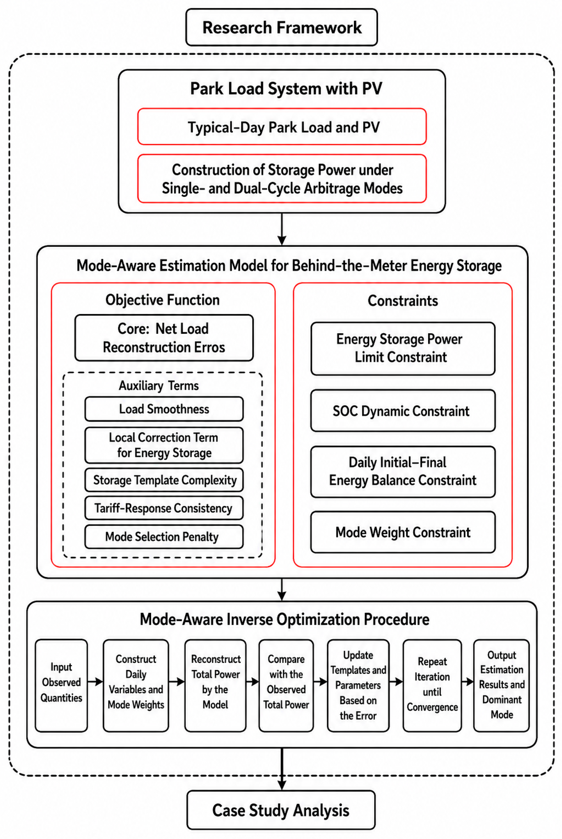
The overall framework of the proposed mode-aware behind-the-meter distributed energy storage power estimation method is shown in Figure 1. The proposed method takes the measured net load power, photovoltaic power, and time-of-use tariff as the available input information. Since the actual user load and the behind-the-meter storage power are not directly observable, the estimation problem is solved by combining mode-aware joint component representation, operational constraints, and constrained inverse optimization.

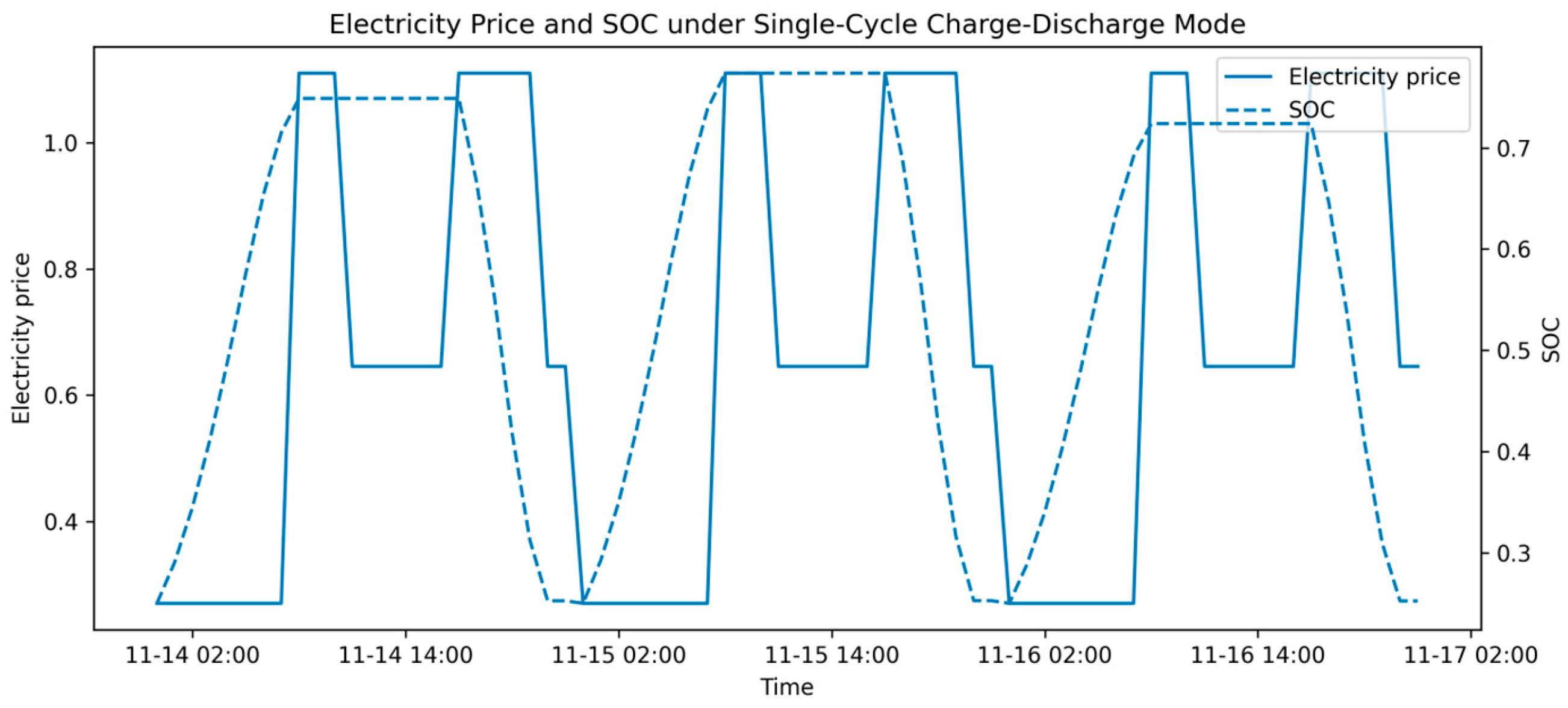
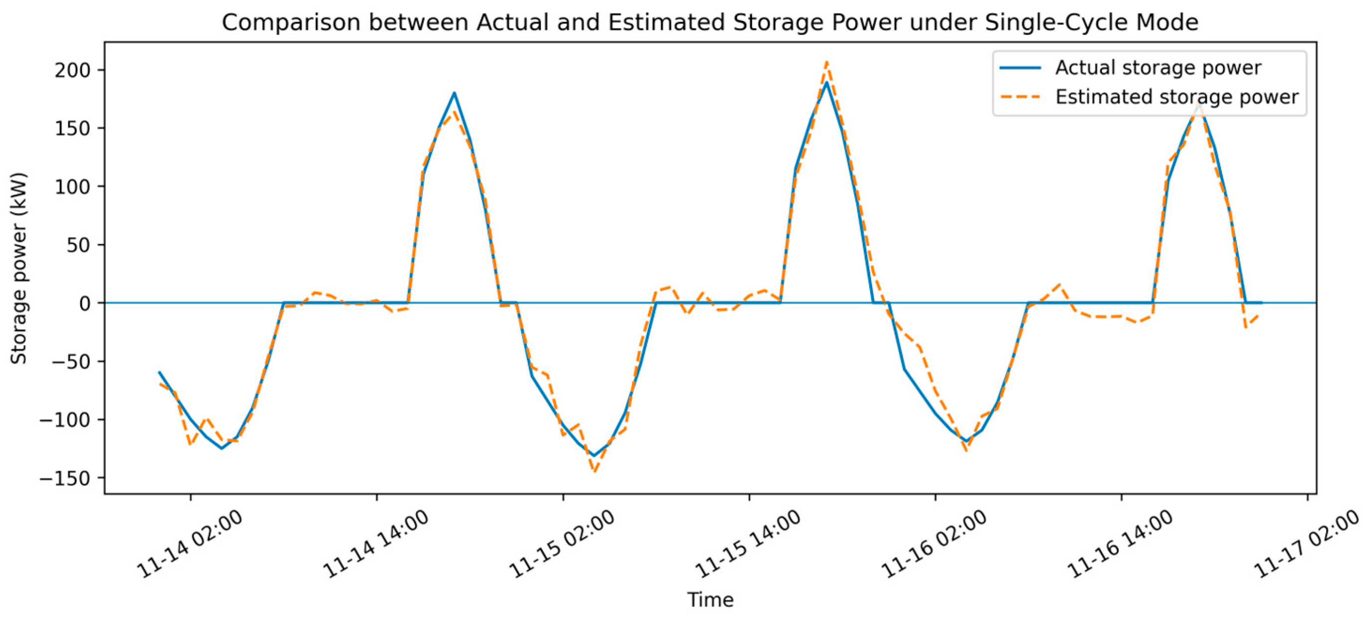
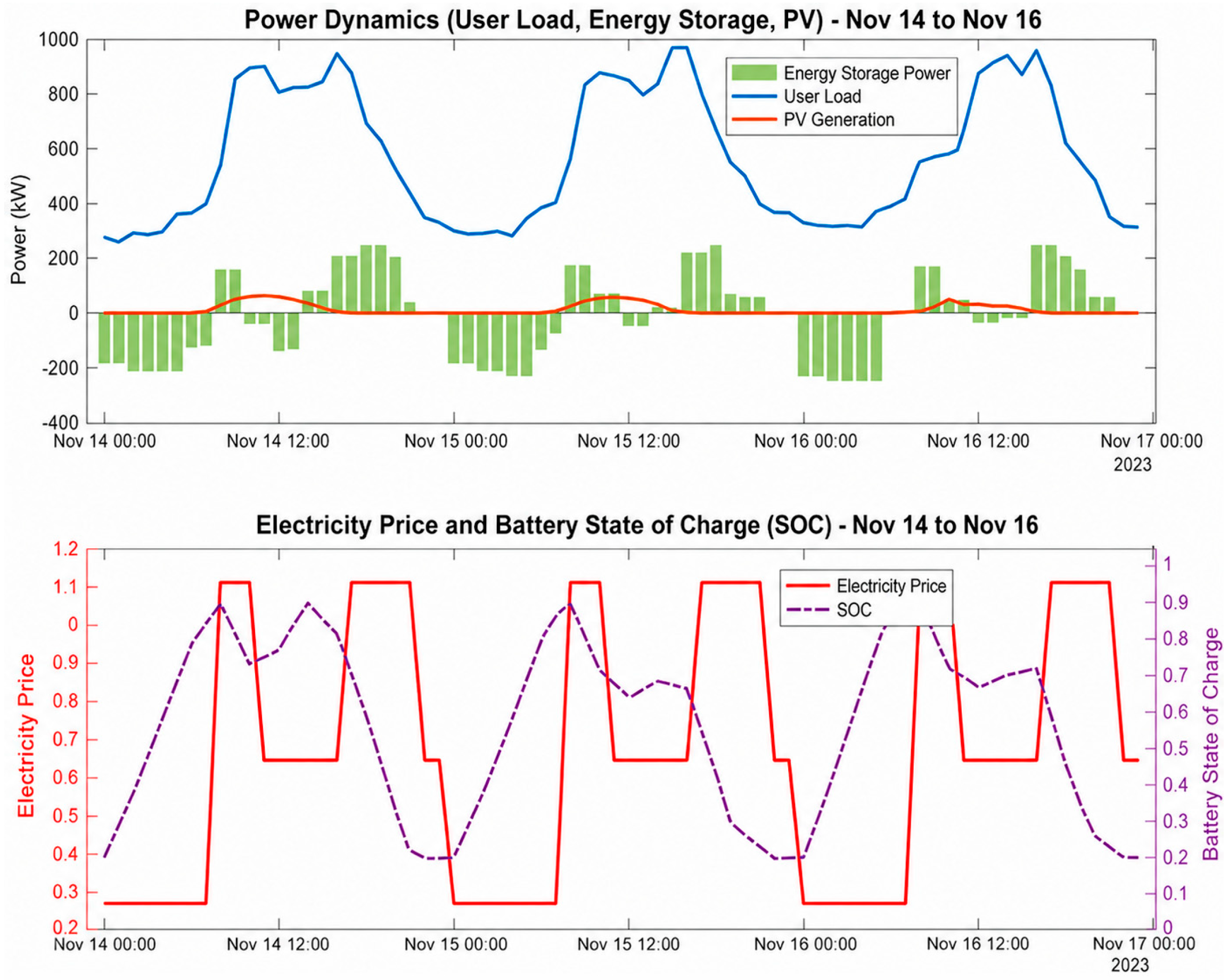
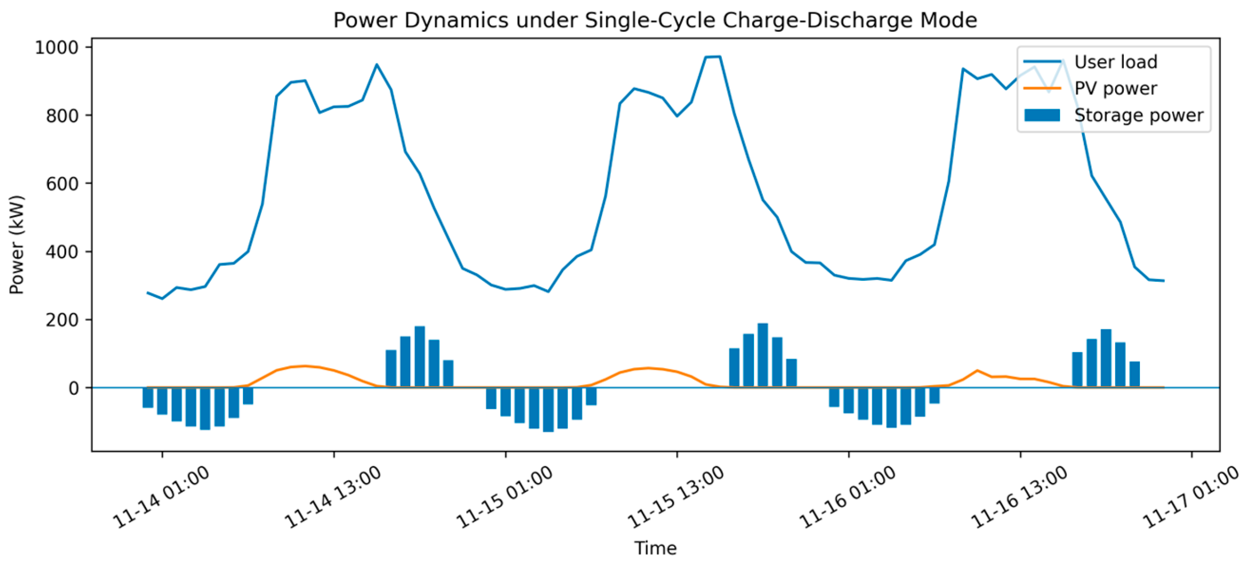
In addition to the common template-based representation, this paper further introduces an arbitrage mode library for behind-the-meter energy storage. Two typical operation modes are considered: the single-cycle charge–discharge mode and the dual-cycle charge–discharge mode. The single-cycle mode represents the case where the storage system charges once during the valley-tariff period and discharges once during the peak-tariff period. The dual-cycle mode represents the case where the storage system performs two charging and two discharging actions within one day according to multiple valley, peak, and critical peak tariff periods.

The two modes are selected according to the storage operation characteristics observed in the studied park-level fixed time-of-use tariff scenario. The single-cycle mode represents the basic peak–valley arbitrage strategy, in which the storage system charges during the valley-tariff period and discharges during the peak-tariff period. The dual-cycle mode represents a more flexible intraday arbitrage strategy under multiple valley, peak, or critical peak tariff periods, where the storage system may perform more than one charging and discharging action within a day. Therefore, the two-mode library is used as a case-specific representation of the main tariff-driven storage behaviors considered in this study, rather than a general mode library for all possible behind-the-meter storage operation strategies.

If the reference storage behavior deviates significantly from the predefined single-cycle and dual-cycle mode library, the local correction terms can partially absorb the mismatch. However, the estimation error may increase, and the estimated mode weights may become less decisive. Therefore, the proposed mode library should be regarded as suitable for the fixed time-of-use arbitrage scenario studied in this paper. More complex storage behaviors, such as demand charge reduction, photovoltaic self-consumption, backup reserve, grid service participation, or manual dispatch, require an extended mode library or additional operation constraints.

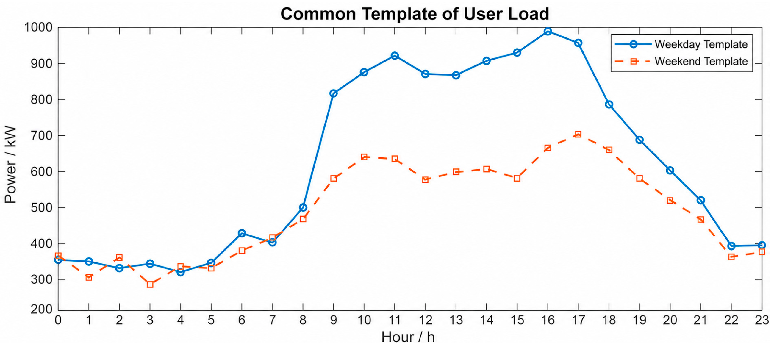
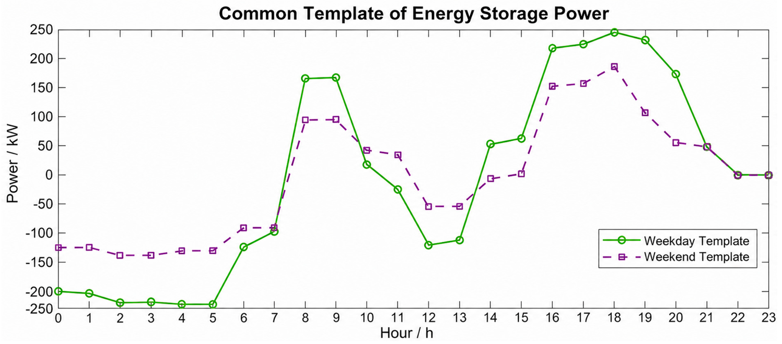
First, the user load and energy storage power are described using a joint representation model. Instead of treating the two components as completely free time-series variables, common daily templates are introduced to represent their typical intraday patterns. Daily scaling factors are used to describe the differences in load level and storage action intensity among different days, and local correction terms are added to compensate for short-term deviations. In addition, weekdays and weekends are modeled separately to reflect their different load patterns and storage operation characteristics.

Second, energy storage operational constraints are embedded into the estimation model. The estimated storage power is required to satisfy charging and discharging power limits, SOC dynamic constraints, SOC boundary constraints, and daily energy balance constraints. These constraints restrict the feasible range of storage power and prevent physically unreasonable estimation results, such as continuous one-way charging or discharging.

Third, a mode-aware inverse optimization model is established. The reconstructed net load is calculated from the estimated user load, photovoltaic power, and estimated storage power, and then compared with the measured net load. The reconstruction error, together with load smoothness, storage local correction penalty, storage template complexity penalty, tariff-response consistency penalty, and mode selection penalty, forms the objective function. During the iterative solution process, the templates, mode weights, daily coefficients, local correction terms, and storage-related variables are updated according to the reconstruction error and operational constraints until convergence is reached.

Therefore, under the studied fixed time-of-use tariff scenario, the proposed method can be summarized as a “mode-aware joint representation–operational constraint–constrained inverse optimization” framework. The final outputs are the estimated user load, behind-the-meter storage power, SOC trajectory, and dominant storage arbitrage mode.

2.3. Mode-Aware Joint Representation of User Load and Storage Power

Under fixed time-of-use tariff conditions, the user load and the operation of behind-the-meter energy storage are not completely random. The user load usually has relatively stable intraday patterns, while the charging and discharging behavior of the energy storage system is closely related to the valley, flat, peak, and critical peak tariff periods. In practical user-side applications, the energy storage system may follow different arbitrage operation patterns. Therefore, this paper introduces a mode-aware joint representation model to describe user load and storage power, in which single-cycle and dual-cycle charge–discharge modes are considered as the mode library for the studied fixed time-of-use tariff scenario.

Considering the differences between weekdays and weekends in load level, peak–valley position, and storage response behavior, two types of daily templates are constructed. The day type of day d is denoted by c_d, where c_d = w represents a weekday and c_d = e represents a weekend. The user load of day d is represented as

$$P_{\mathrm{load}}(d,h)=a_d{L}_{\mathrm{temp}}^c(d,h)+\Delta L(d,h),$$

(2)

where $L_{\mathrm{temp}}^c(d,h)$ is the common user load template corresponding to day type c_d, a_d is the daily scaling coefficient of user load, and $∆L(d,h)$ is the local correction term of user load. The common template describes the typical intraday variation pattern of user load, the daily scaling coefficient reflects the overall load level of each day, and the local correction term compensates for short-term fluctuations that cannot be described by the common template.

Different from the conventional single-template representation, this paper introduces a storage arbitrage mode library to describe different charging and discharging behaviors under time-of-use tariffs. Let M = {m1, m2}, where m1 denotes the single-cycle charge–discharge mode and m2 denotes the dual-cycle charge–discharge mode. The storage power of the d-th day is represented as

$$P_{\mathrm{ES}}(d,h)=b_d\left[{\rho }_{d,1}{E}_{\mathrm{temp}}^{c,1}(d,h)+{\rho }_{d,2}{E}_{\mathrm{temp}}^{c,2}(d,h)\right]+\Delta E(d,h),$$

(3)

where $E_{\mathrm{temp}}^{c,1}(d,h)$ is the storage power template of the single-cycle charge–discharge mode, $E_{\mathrm{temp}}^{c,2}(d,h)$ is the storage power template of the dual-cycle charge–discharge mode, $b_d$ is the daily action intensity coefficient of storage operation, ${\rho }_{d,1}$ and ${\rho }_{d,2}$ are the mode weights of the d-th day, and $∆E(d,h)$ is the local correction term of storage power. The mode weights satisfy

$$0\le {\rho }_{d,1}\le 1, 0\le {\rho }_{d,2}\le 1,$$

(4)

$${\rho }_{d,1}+{\rho }_{d,2}=1,$$

(5)

The dominant storage mode of day d is determined according to the larger mode weight. If ${\rho }_{d,1}$ $\ge$ ${\rho }_{d,2}$, the dominant mode is identified as the single-cycle mode; otherwise, it is identified as the dual-cycle mode.

The single-cycle mode describes the case where the storage system charges once during the valley-tariff period and discharges once during the peak-tariff period. The dual-cycle mode describes the case where the storage system performs two charging and two discharging actions within one day according to multiple valley, peak, and critical peak tariff periods. Under the studied fixed time-of-use tariff scenario, the proposed representation can estimate the storage power and provide an interpretable indicator of the dominant daily arbitrage mode through the mode weights.

This mode-aware joint representation has three main advantages. First, it reduces the degrees of freedom of the estimation problem by using common templates to represent the typical daily patterns of user load and storage power. Second, it retains sufficient flexibility through daily coefficients and local correction terms, so that day-to-day differences and local variations can still be described. Third, the mode weights provide an interpretable indicator of the daily storage arbitrage mode. Therefore, the proposed model avoids directly treating the hidden components as completely free time-series variables and helps improve the stability and interpretability of behind-the-meter storage power estimation.

2.4. Energy Storage Operational Constraints

Although the joint representation model in Section 2.3 reduces the degrees of freedom of the estimation problem, the estimated storage power may still be physically unreasonable if no operational constraints are imposed. In practical operation, behind-the-meter energy storage is limited by its charging and discharging power capability, energy capacity, SOC operating range, and daily operation strategy. Therefore, energy storage operational constraints are introduced to ensure that the estimated storage power satisfies basic physical and operational feasibility requirements.

First, the charging and discharging power of the energy storage system should not exceed its rated power limits. The power limit constraint is expressed as

$$-P_{\mathrm{ch},\max }\le P_{\mathrm{ES}}(d,h)\le P_{\mathrm{dis},\max },$$

(6)

where $P_{ch,max}$ and $P_{\mathrm{dis},max}$ denote the maximum charging power and maximum discharging power, respectively. In this paper, positive $P_{\mathrm{ES}}(d,h)$ represents discharging, while negative $P_{\mathrm{ES}}(d,h)$ represents charging.

To describe the charging and discharging process more clearly, the storage power is further decomposed into the discharging power and charging power:

$$P_{\mathrm{ES}}(d,h)=P_{\mathrm{dis}}(d,h)-P_{\mathrm{ch}}(d,h),$$

(7)

where $P_{ch}(d,h)$ and $P_{dis}(d,h)$ denote the charging and discharging powers, respectively.

$$0\le P_{\mathrm{ch}}(d,h)\le P_{\mathrm{ch},\max },$$

(8)

$$0\le P_{\mathrm{dis}}(d,h)\le P_{\mathrm{dis},\max },$$

(9)

To avoid physically unrealistic simultaneous charging and discharging, an additional simultaneous charge–discharge penalty is introduced:

$$J_{\mathrm{cd}}={\displaystyle \sum _{d=1}^D}{\displaystyle \sum _{h=1}^H}{P}_{\mathrm{ch}}(d,h)P_{\mathrm{dis}}(d,h),$$

(10)

This term penalizes the overlap between charging power and discharging power. When either $P_{ch}(d,h)$ or $P_{dis}(d,h)$ is close to zero at each time interval, J_cd becomes small. Therefore, this term encourages the storage system to operate in either charging, discharging, or standby state, rather than charging and discharging simultaneously. The penalty J_cd is further included in the total objective function in Section 2.5.

Second, the SOC evolution of the energy storage system is considered. The SOC at the next time interval is determined by the current SOC, charging power, discharging power, charging efficiency, discharging efficiency, and sampling interval. The SOC dynamic equation is given by

$$SOC(d,h+1)=SOC(d,h)+{\displaystyle \frac{{\eta }_{\mathrm{ch}}{P}_{\mathrm{ch}}(d,h)\Delta t}{E_{\mathrm{ES}}}}-{\displaystyle \frac{P_{\mathrm{dis}}(d,h)\Delta t}{{\eta }_{\mathrm{dis}}{E}_{\mathrm{ES}}}},$$

(11)

where $SOC(d,h)$ denotes the state of charge of the energy storage system on day d at time interval h, $E_{\mathrm{ES}}$ denotes the available energy capacity, ${\eta }_{\mathrm{ch}}$ and ${\eta }_{\mathrm{dis}}$ denote the charging and discharging efficiencies, respectively, and Δt denotes the sampling interval.

Third, the SOC should remain within a reasonable operating range to avoid overcharging and overdischarging. The SOC boundary constraint is expressed as

$$SO{C}_{\min }\le SOC(d,h)\le SO{C}_{\max },$$

(12)

where ${SOC}_{min}$ and ${SOC}_{max}$ denote the lower and upper SOC limits, respectively.

Finally, a daily energy balance constraint is introduced. For a behind-the-meter storage system operating under a typical daily cycle, the SOC at the end of a day is expected to return to approximately the initial SOC level. Therefore, the following constraint is imposed:

$$SOC(0)=SOC(d,H),$$

(13)

where H denotes the number of time intervals in one day. In the case study, SOC_min is set to 0.1, SOC_max is set to 0.9, and the initial SOC is set to SOC₀ = 0.2. This constraint prevents the model from continuously charging or discharging the storage system only to improve the net load reconstruction accuracy. By introducing the above constraints, the estimated storage power is not only required to explain the observed net load, but also required to satisfy the basic operation mechanism of energy storage.

In addition to the physical operation constraints, a tariff-response consistency penalty is introduced to reflect the economic operation mechanism of behind-the-meter energy storage. During valley-tariff periods, the storage system is expected to charge rather than discharge. During peak and critical peak periods, the storage system is expected to discharge rather than charge. Therefore, the tariff-response consistency penalty is defined as

$$J_{\mathrm{tariff}}=\sum _{h\in {\mathcal{T}}_v}{\left[\max (P_{\mathrm{ES}}(d,h),0)\right]}^2+\sum _{h\in {\mathcal{T}}_p}{\left[\max (-P_{\mathrm{ES}}(d,h),0)\right]}^2,$$

(14)

where ${\mathcal{T}}_v$ denotes the valley-tariff period, and ${\mathcal{T}}_p$ denotes the peak or critical peak tariff period. This term penalizes discharging during low-tariff periods and charging during high-tariff periods so that the estimated storage power can better follow the basic arbitrage logic under time-of-use tariffs.

2.5. Objective Function and Inverse Optimization Procedure

Based on the mode-aware joint representation model and energy storage operational constraints described above, an inverse optimization model is established to estimate the user load, behind-the-meter energy storage power [19,20], and dominant storage arbitrage mode. The objective function is designed to ensure that the reconstructed net load is close to the measured net load, while the estimated load and storage components remain smooth, stable, and physically reasonable.

Before constructing the total objective function, different objective terms are normalized to reduce the scale difference among reconstruction error, smoothness penalty, correction penalty, template complexity penalty, tariff-response penalty, mode selection penalty, and simultaneous charge–discharge penalty. The reconstruction error is treated as the dominant term, while the other terms are used as regularization terms to improve physical feasibility and estimation stability.

First, the net load reconstruction error is defined as

$$J_{\mathrm{rec}}={\displaystyle \sum _{d=1}^D}{\displaystyle \sum _{h=1}^H}{\left[P_{\mathrm{grid}}(d,h)-P_{\mathrm{grid}}^{\mathrm{rec}}(d,h)\right]}^2,$$

(15)

where D is the number of days in the dataset, H is the number of time intervals in one day, and $P_{\mathrm{grid},d}^{\mathrm{rec}}(h)$ is the reconstructed net load, which is given by

$$P_{\mathrm{grid}}^{\mathrm{rec}}(d,h)=P_{\mathrm{load}}(d,h)-P_{\mathrm{PV}}(d,h)-P_{\mathrm{ES}}(d,h),$$

(16)

The term $J_{\mathrm{rec}}$ is the core part of the objective function. It forces the estimated user load and energy storage power to explain the measured net load as accurately as possible.

Second, a load smoothness term is introduced to avoid unreasonable high-frequency fluctuations in the estimated user load:

$$J_{\mathrm{load}}={\displaystyle \sum _{d=1}^D}{\displaystyle \sum _{h=2}^H}{\left[P_{\mathrm{load}}(d,h)-P_{\mathrm{load}}(d,h-1)\right]}^2,$$

(17)

Since user load usually changes gradually within a short time interval, this term helps improve the rationality of the estimated load curve.

Third, a storage local correction penalty is introduced to prevent the storage power estimation from relying excessively on local correction terms:

$$J_{\mathrm{corr}}={\displaystyle \sum _{d=1}^D}{\displaystyle \sum _{h=1}^H}{\left[\Delta E(d,h)\right]}^2,$$

(18)

This term limits the magnitude of local corrections and prevents the estimated storage power from becoming overly irregular.

Fourth, a storage template complexity penalty is used to constrain the fluctuation of the storage power template:

$$J_{\mathrm{temp}}={{\displaystyle \sum }}_{h=2}^H{\left[E_{\mathrm{temp}}^{c,1}(d,h)-E_{\mathrm{temp}}^{c,1}(d,h-1)\right]}^2+{{\displaystyle \sum }}_{h=2}^H{\left[E_{\mathrm{temp}}^{c,2}(d,h)-E_{\mathrm{temp}}^{c,2}(d,h-1)\right]}^2,$$

(19)

This term prevents the common storage template from becoming too fragmented and helps retain the typical charging and discharging pattern under time-of-use tariffs.

To avoid ambiguous mixing between different arbitrage modes, a mode selection penalty is introduced as

$$J_{\mathrm{mode}}={\displaystyle \sum _{d=1}^D}\left[{\rho }_{d,1}(1-{\rho }_{d,1})+{\rho }_{d,2}(1-{\rho }_{d,2})\right],$$

(20)

Therefore, the total objective function can be formulated as

$$\min J={\lambda }_1{J}_{\mathrm{rec}}+{\lambda }_2{J}_{\mathrm{load}}+{\lambda }_3{J}_{\mathrm{corr}}+{\lambda }_4{J}_{\mathrm{temp}}+{\lambda }_5{J}_{\mathrm{tariff}}+{\lambda }_6{J}_{\mathrm{mode}}+{\lambda }_7{J}_{\mathrm{cd}},$$

(21)

where $J_{\mathrm{rec}}$ is the net load reconstruction error, $J_{\mathrm{load}}$ is the user load smoothness penalty, $J_{\mathrm{corr}}$ is the storage local correction penalty, $J_{\mathrm{temp}}$ is the storage template complexity penalty, $J_{\mathrm{tariff}}$ is the tariff-response consistency penalty, $J_{\mathrm{mode}}$ is the mode selection penalty, and $J_{\mathrm{cd}}$ are weighting parameters used to balance different objective terms after normalization. The coefficients ${\lambda }_1-{\lambda }_7$ are weighting parameters used to balance different objective terms.

The decision variable set in the training stage is defined as

$${\mathrm{\Xi }}_{\mathrm{tr}}=\left\{\begin{array}{c}{L}_{\mathrm{temp}}^c,E_{\mathrm{temp}}^{c,1},E_{\mathrm{temp}}^{c,2},a_d,b_d,{\rho }_{d,1},{\rho }_{d,2},\Delta L(d,h),\\ \Delta E(d,h),P_{\mathrm{ES}}(d,h),SOC(d,h),{\mathrm{\Theta }}_{\mathrm{ES}}\end{array}\right\},$$

(22)

where $L_{\mathrm{temp}}^c$ is the user load template, $E_{\mathrm{temp}}^{c,1}$ and $E_{\mathrm{temp}}^{c,2}$ are the single-cycle and dual-cycle storage templates, respectively, ${\rho }_{d,1}$ and ${\rho }_{d,2}$ are the mode weights, and ${\mathrm{\Theta }}_{\mathrm{ES}}$ denotes the storage-related parameter set.

Here ${\mathrm{\Theta }}_{\mathrm{ES}}$ denotes the storage-related parameter set.

The unified optimization model in the training stage can be expressed as

$$\begin{array}{c}\underset{{\mathrm{\Xi }}_{\mathrm{tr}}}{\min }{\lambda }_1{J}_{\mathrm{rec}}+{\lambda }_2{J}_{\mathrm{load}}+{\lambda }_3{J}_{\mathrm{corr}}+{\lambda }_4{J}_{\mathrm{temp}}+{\lambda }_5{J}_{\mathrm{tariff}}+{\lambda }_6{J}_{\mathrm{mode}}+{\lambda }_7{J}_{\mathrm{cd}}\\ \mathrm{s}.\mathrm{t}.P_{\mathrm{ES}}(d,h),SOC(d,h)\in {\mathrm{\Phi }}_{\mathrm{ES}}({\mathrm{\Theta }}_{\mathrm{ES}}),\\ 0\le {\rho }_{d,1}\le 1, 0\le {\rho }_{d,2}\le 1,\\ {\rho }_{d,1}+{\rho }_{d,2}=1,\\ d=1,\dots ,D, h=1,\dots ,H.\end{array},$$

(23)

The feasible set Phi includes the power balance equation, charging and discharging power limits, storage power decomposition, SOC dynamic equation, SOC bounds, daily SOC balance, mode-weight constraints, bounds of daily scaling coefficients, bounds of local correction terms, and the storage-related parameter ranges. Therefore, Phi defines the feasible operation region of the estimated behind-the-meter storage system.

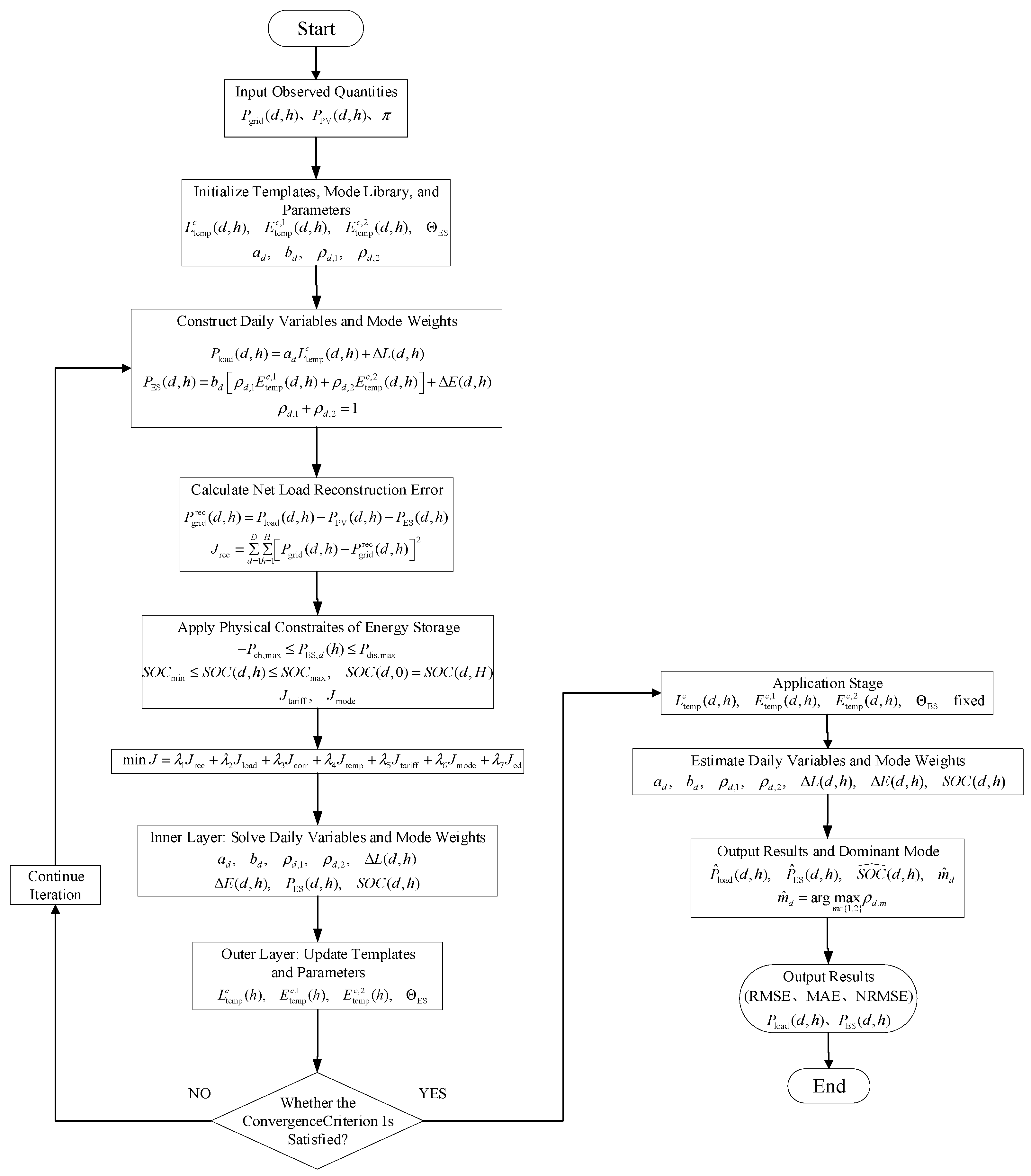
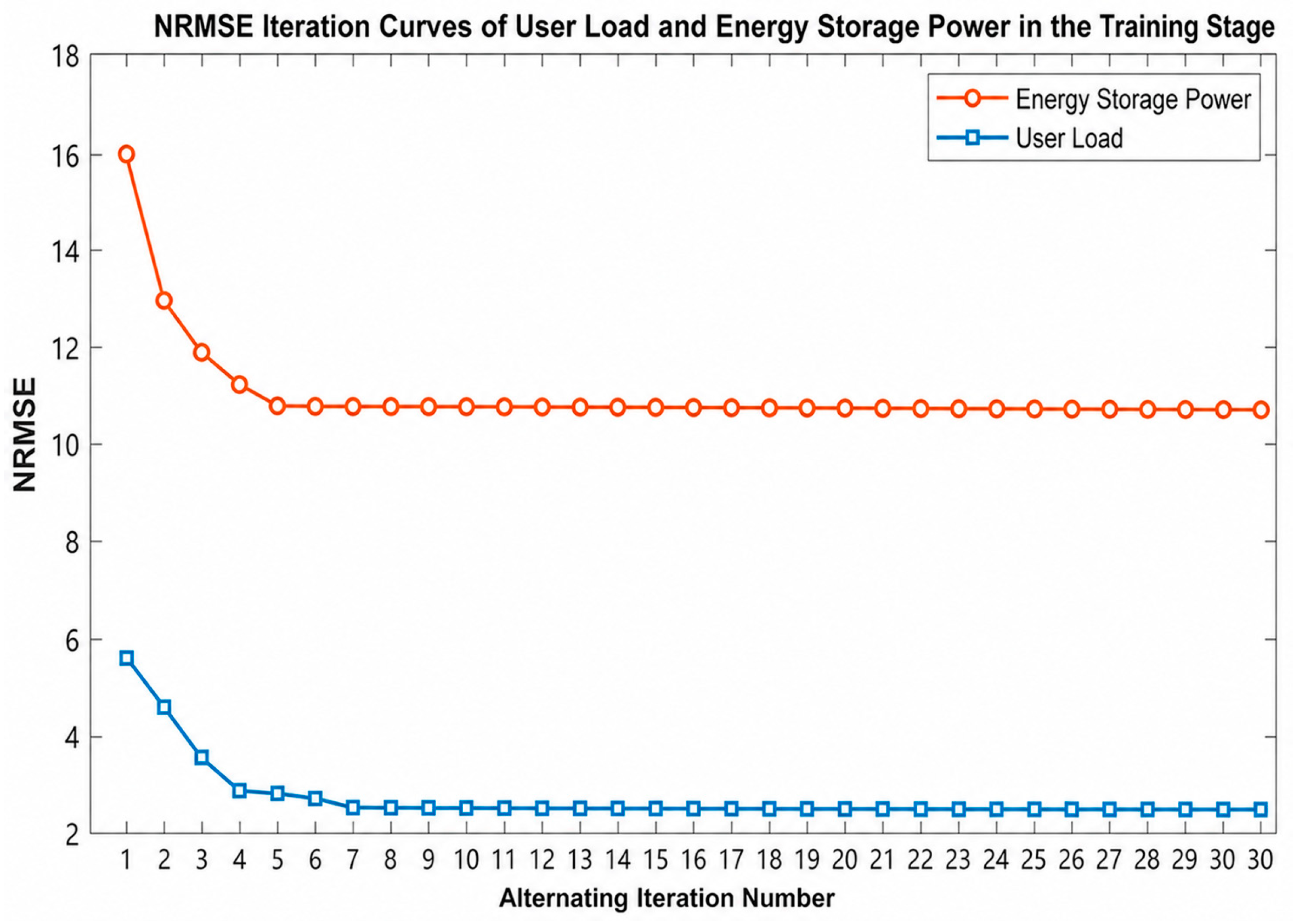
Since the optimization variables include the user load template, mode-dependent storage templates, daily coefficients, mode weights, local correction terms, storage power, SOC trajectories, and storage parameters, directly solving the whole optimization problem may lead to high dimensionality and unstable convergence. Therefore, an alternating iterative solution strategy is adopted. The training process includes the following steps:

• Initialize the user load template, the single-cycle storage template, the dual-cycle storage template, and storage-related parameters.
• Estimate the daily coefficients, local correction terms, storage power, SOC trajectory, and mode weights for each training day.
• Identify the dominant arbitrage mode of each day according to the estimated mode weights.
• Update the user load template and the mode-dependent storage templates.
• Update the storage-related parameters under the operational constraints.
• Calculate the objective function and check the convergence condition.
• Repeat the above steps until the objective function converges or the maximum number of iterations is reached.

After training, the learned user load template, mode-dependent storage templates, mode-weight ranges, and storage-related parameter ranges are fixed. In the testing stage, only the measured net load, photovoltaic power, and time-of-use tariff information of the testing days are used as inputs. The user load, behind-the-meter storage power, SOC trajectory, and dominant storage arbitrage mode are then estimated by solving the same mode-aware inverse optimization problem under the trained templates and operational constraints. The overall mode-aware inverse optimization procedure is summarized in Figure 2.

To improve the reproducibility of the proposed inverse optimization procedure, the main implementation settings are summarized in

Table 1. Main implementation settings of the proposed method.

Item	Setting
Programming environment	MATLAB R2024b (The MathWorks, Inc., Natick, MA, USA)
Solver	fmincon with SQP algorithm
Optimization strategy	Alternating iterative optimization
Objective normalization	Each objective term was normalized by its initial value
Maximum iterations	100
Convergence tolerance	1.0 × 10−4
Stopping criterion	Relative change in the objective function below the tolerance or maximum iterations reached
Initialization	Load template: average daily load; storage templates: initialized according to TOU periods; mode weights: 0.5/0.5; local corrections: 0
Objective weights	λ1 = 1.00, λ2 = 0.10, λ3 = 0.20, λ4 = 0.05, λ5 = 0.15, λ6 = 0.05, λ7 = 0.20
Average runtime	About 4.3 min for one training run and 0.8 min for one testing run
Computational platform	Intel Core i7 CPU, 16 GB RAM, Windows 11
Local-minimum treatment	The model was initialized from average load profiles and tariff-based storage templates; repeated runs with the same setting showed stable convergence

. All objective terms were normalized before weighting, and the same settings were used in the main dual-cycle case and the supplemental single-cycle case.

The reconstruction-error weight was set as the dominant term, while the other weights were used as regularization terms to improve load smoothness, storage feasibility, tariff-response consistency, mode interpretability, and suppression of simultaneous charging and discharging.

The computational complexity mainly increases with the number of days D, the number of time intervals H, and the number of decision variables in the daily subproblem. Since the case study uses 40 days with a 1 h resolution, the computational burden is acceptable for offline estimation.

3. Results

3.1. Case Study Description

To verify the proposed mode-aware behind-the-meter energy storage power estimation method, a case study was conducted using a hybrid dataset constructed from park-level user load data, photovoltaic output data, and reconstructed energy storage operation profiles. The user load and photovoltaic power were obtained from park-level operation data, while the behind-the-meter storage power was reconstructed according to typical time-of-use tariff arbitrage behaviors. Therefore, the storage power used for performance evaluation was not directly measured from a physical battery system, but was generated according to predefined storage operation rules under the given tariff structure.

In the main case, the reconstructed storage operation follows a dual-cycle charge–discharge pattern, in which the storage system charges during low-tariff periods and discharges during peak or critical peak periods. This main case is used to evaluate the estimation performance of the proposed method under the studied fixed time-of-use tariff scenario. In addition, a supplemental single-cycle charge–discharge case is constructed in Section 3.3 by keeping the same user load, photovoltaic power, and tariff profile, while reconstructing the storage power according to a simpler single-cycle arbitrage pattern. The supplemental case is used to examine the representation capability of the proposed mode library, rather than to claim general adaptability to all possible storage operation behaviors.

The measured net load power, photovoltaic power, and time-of-use tariff were used as the input information of the proposed inverse optimization model. The actual user load and reconstructed storage power were not used as direct labels during the estimation process. They were only used as reference values for evaluating the estimation accuracy. Therefore, the case study reflects an incomplete-measurement scenario in which the behind-the-meter storage power is hidden in the observed net load from the perspective of the distribution system operator.

The typical daily curves of user load, photovoltaic power, and energy storage power are shown in Figure 3. It can be observed that the photovoltaic power mainly appears during daytime, while the storage power shows obvious charging and discharging behavior under the influence of the time-of-use tariff. This provides a data basis for verifying whether the proposed method can recover the hidden storage power component from the measured net load.

The main parameters of the behind-the-meter energy storage system are listed in

Table 2. Parameters of the behind-the-meter energy storage system.

Parameter	Value
Maximum charging power	247.23 kW
Maximum discharging power	247.23 kW
Available capacity	1.4 MWh
Charging/discharging efficiency	0.95
SOC lower bound	0.1
SOC upper bound	0.9
Initial SOC	0.2

. These parameters are used to define the feasible operation region of the energy storage system, including charging and discharging power limits, available energy capacity, and charging/discharging efficiency.

The fixed time-of-use tariff used in this case study consists of valley, flat, peak, and critical peak periods. The valley period is 00:00–08:00 with a tariff of 0.2699 CNY/kWh. The peak periods are 08:00–09:00, 17:00–18:00, and 20:00–22:00 with a tariff of 1.1091 CNY/kWh. The critical peak periods are 09:00–11:00 and 18:00–20:00 with a tariff of 1.3309 CNY/kWh. The flat periods are 11:00–17:00 and 22:00–24:00 with a tariff of 0.6450 CNY/kWh.

3.2. Template Estimation Results

The estimated user load template and the dominant storage power template obtained from the training data are shown in Figure 4 and Figure 5, respectively. The user load template reflects the typical intraday variation pattern of the park load. Since the training data of the main case are dominated by dual-cycle charge–discharge behavior, the storage template shown in Figure 5 corresponds to the dominant dual-cycle arbitrage mode learned from the training data.

Figure 5 shows the dominant dual-cycle template of behind-the-meter energy storage power. Compared with the user load template, the storage power template presents a more obvious segmented charging and discharging pattern. Under fixed time-of-use tariff conditions, the storage system tends to charge during valley-tariff periods and discharge during peak or critical peak periods. Therefore, the estimated dual-cycle storage template is consistent with the typical peak-shaving and valley-filling operation mechanism of user-side energy storage.

To quantify the distribution of storage operation modes in the training stage, the mode statistics are summarized in

Table 3. Mode distribution and template stability in the training stage.

Item	Value
Total training days	30
Weekday/weekend days	22/8
Single-cycle dominant days	5
Dual-cycle dominant days	25
Average single-cycle weight	0.23
Average dual-cycle weight	0.77
Average storage-template residual	18.64 kW
Standard deviation of storage-template residual	7.92 kW
Maximum storage-template residual	46.27 kW

.

As shown in Table 3, 25 of the 30 training days are identified as dual-cycle dominant days. The average dual-cycle weight is 0.77, which quantitatively supports that the main training case is dominated by dual-cycle storage operation. The residual mean, standard deviation, and maximum value are also reported to quantify the stability of the learned storage template without adding an additional confidence-band figure.

Since the training data are dominated by dual-cycle charge–discharge behavior, Figure 5 mainly presents the dominant dual-cycle storage template. The single-cycle template is retained in the proposed mode library, and its representation capability is further examined through the supplemental single-cycle case in Section 3.3.

The above results indicate that the mode-aware joint representation model can capture the main regular patterns of both user load and storage power. The common user load template and the mode-dependent storage templates describe the shared intraday characteristics, while the daily scaling factors, mode weights, and local correction terms further compensate for day-to-day differences.

3.3. Verification Under Single-Cycle Charge Discharge Mode

Following the template analysis in Section 3.2, this subsection examines the single-cycle mode contained in the proposed storage mode library. This supplemental case is used as a controlled test to evaluate whether the proposed mode-aware representation can describe a simpler single-cycle arbitrage behavior. The main quantitative evaluation of the proposed method is still conducted under the dual-cycle testing case in Section 3.4.

To examine the representation capability of the proposed mode library, a supplemental single-cycle charge–discharge case was constructed based on the original dataset. In this case, the user load, photovoltaic power, and time-of-use tariff were kept unchanged, while the reference storage power was reconstructed according to a single-cycle arbitrage pattern. Specifically, the storage system charges once during the night valley-tariff period and discharges once during the evening peak-tariff period. The net load and SOC trajectory were then recalculated according to the power balance relationship and SOC dynamic equation.

Figure 6 shows the power dynamics under the single-cycle charge–discharge mode. Compared with the main dual-cycle case, the storage power in this supplemental case presents only one charging period and one discharging period within each day. The charging process mainly occurs during the night valley-tariff period, while the discharging process is concentrated in the evening peak period. This operation pattern is consistent with the basic logic of peak–valley arbitrage and evening peak shaving.

Figure 7 shows the electricity price and SOC trajectory under the single-cycle charge–discharge mode. It can be observed that the SOC increases during the night charging period and decreases during the evening discharging period. During the daytime standby period, the SOC remains almost unchanged. This indicates that the constructed single-cycle case can reflect a typical daily charge–discharge behavior of user-side energy storage.

Figure 8 compares the reference and estimated storage power under the single-cycle mode. The estimated storage power can follow the main charging and discharging trend of the reference storage power, indicating that the proposed mode-aware representation can describe the main pattern of the constructed single-cycle arbitrage case. However, this supplemental case is a controlled test based on reconstructed storage operation rather than an independent validation using measured battery data. Therefore, it is used to support the representation capability of the proposed mode library, rather than to claim general adaptability to all storage operation scenarios.

To provide quantitative evidence in addition to the visual comparison, the estimation errors of the supplemental single-cycle case are summarized in

Table 4. Error evaluation of the supplemental single-cycle case.

Metric	Value
RMSE of storage power	12.07 kW
MAE of storage power	9.71 kW
NRMSE of storage power	3.77%
Energy throughput error	3.90%
Identified dominant mode	Single-cycle
Single-cycle mode weight	0.84
Dual-cycle mode weight	0.16

.

The storage power RMSE, MAE, and NRMSE are 12.07 kW, 9.71 kW, and 3.77%, respectively. The single-cycle mode weight is 0.84, which is much larger than the dual-cycle mode weight of 0.16. This indicates that the proposed mode-aware representation identifies the supplemental case as single-cycle dominant, which is consistent with the constructed storage operation pattern.

As shown in

Table 5. Mode weights and identified arbitrage modes.

Case	Single-Cycle Weight	Dual-Cycle Weight	Identified Mode
Supplemental single-cycle case	0.84	0.16	Single-cycle
Main dual-cycle case	0.21	0.79	Dual-cycle

, the supplemental single-cycle case has a larger single-cycle mode weight, while the main testing case is dominated by the dual-cycle mode. This result indicates that the estimated mode weights can reflect the dominant operation pattern in the constructed single-cycle and dual-cycle cases.

3.4. Main Testing Results Under Dual-Cycle Operation

The training and testing estimation results of the main dual-cycle case are analyzed in this section to evaluate the convergence behavior and testing performance of the proposed method under the studied fixed time-of-use tariff scenario. In the training stage, the user load template, mode-dependent storage templates, daily coefficients, mode weights, local correction terms, and storage-related variables are updated iteratively according to the net load reconstruction error, tariff-response consistency, mode selection penalty, simultaneous charge–discharge penalty, and energy storage operational constraints.

As shown in Figure 9, the NRMSEs of both user load and storage power decrease rapidly in the first several iterations and then gradually become stable. This indicates that the alternating iterative optimization process can effectively update the common templates and daily variables. The convergence criterion and maximum iteration number are kept consistent with the implementation settings used in the training stage.

After the training stage, the learned templates and storage-related parameters are fixed and applied to the testing days. In the testing stage, only the measured net load, photovoltaic power, and time-of-use tariff are used as input information. The reference user load and storage power are not used in the estimation process, but only serve as reference values for performance evaluation.

Figure 10 shows the testing-stage estimation results of user load and energy storage power. It can be observed that the estimated user load follows the overall variation trend of the reference user load. The estimated storage power can also reflect the main charging and discharging behavior under time-of-use tariff conditions. However, compared with user load estimation, storage power estimation has larger local deviations in some time intervals. This is mainly because storage power has bidirectional charging/discharging characteristics and may switch between charging, discharging, and standby states, making it more difficult to estimate than the relatively smoother user load. For the main testing period, the estimated storage power mainly follows a dual-cycle charge–discharge pattern, which is consistent with the reconstructed dual-cycle reference profile under the adopted time-of-use tariff.

Figure 11 presents the net load reconstruction results in the testing stage. The reconstructed net load is obtained from the estimated user load, photovoltaic power, and estimated storage power. It can be seen that the reconstructed net load is close to the measured net load, indicating that the proposed method can reasonably explain the observed net load through the estimated hidden components. This result indicates that the proposed inverse optimization method can reasonably explain the observed net load through the estimated hidden components under the studied incomplete-measurement scenario.

To further evaluate the effectiveness of the proposed inverse optimization method, two typical data-driven methods, namely multilayer perceptron (MLP) and support vector machine (SVM), were selected as comparison methods. The training and testing sets used for the comparison methods were kept consistent with those of the proposed method, and the same error evaluation indicators were adopted.

It should be noted that MLP and SVM are used as supervised reference models rather than strictly equivalent baselines. During the training process, the reference user load and reconstructed storage power are used as labels for MLP and SVM. In contrast, the proposed method does not directly use storage power labels in the estimation stage, but estimates the hidden components using measured net load, photovoltaic power, time-of-use tariff information, and operational constraints. Therefore, this comparison is used to provide a reference against typical data-driven fitting methods, rather than to claim a fully identical information setting.

The comparison results are shown in Figure 12. It can be observed that the error distribution of the proposed method is more concentrated than those of MLP and SVM in both the training and testing stages. The proposed method shows a lower median error and a smaller fluctuation range, indicating better estimation stability. This result demonstrates that introducing operational constraints and inverse optimization can improve the robustness of behind-the-meter energy storage power estimation when direct storage power measurements are unavailable.

Compared with pure data-driven methods, the proposed method has stronger physical interpretability. The estimated storage power is constrained by charging and discharging power limits, SOC dynamics, SOC bounds, and daily energy balance. Therefore, the estimation results are not only fitted to the observed net load, but also consistent with the basic operating mechanism of energy storage. This is the main reason why the proposed method achieves better stability and generalization performance in the comparison.

3.5. Error Evaluation

To quantitatively evaluate the performance of the proposed method, RMSE, MAE, and NRMSE were adopted as error indicators. RMSE reflects the overall deviation between the estimated and reference values, MAE reflects the average absolute estimation error, and NRMSE is used to compare the relative error levels of different power components. In this paper, NRMSE is calculated by normalizing RMSE with the range of the corresponding reference signal. The evaluation results of energy storage power, user load, and net load in both the training and testing stages are listed in

Table 6. Error evaluation results of the proposed method.

Object	Stage	RMSE/kW	MAE/kW	NRMSE/%
Energy storage power	Training	25.17	18.12	10.21
Energy storage power	Testing	36.23	27.17	14.75
User load	Training	29.80	21.10	2.39
User load	Testing	40.97	29.38	3.90
Net load	Training	24.65	17.74	2.07
Net load	Testing	37.73	25.57	3.76

.

As shown in Table 6, the proposed method achieves good estimation performance in both the training and testing stages. For energy storage power, the RMSE values in the training and testing stages are 25.17 kW and 36.23 kW, respectively, and the corresponding NRMSE values are 10.21% and 14.75%. For user load, the RMSE values in the training and testing stages are 29.80 kW and 40.97 kW, respectively, while the NRMSE values are 2.39% and 3.90%. For net load reconstruction, the testing-stage RMSE and NRMSE are 37.73 kW and 3.76%, respectively.

The error of energy storage power is higher than those of user load and net load. This is mainly because energy storage power is affected by time-of-use tariffs, SOC constraints, and power limits. It has bidirectional charging/discharging characteristics and local switching behavior, which makes its estimation more difficult than the relatively smoother user load. In addition, the overall magnitude of storage power is smaller than that of user load. Therefore, the same absolute error may result in a higher relative error when NRMSE is used.

In contrast, user load has a more obvious daily periodic pattern, and the net load is the aggregated result of multiple components. Therefore, their relative errors are lower. The testing-stage NRMSE of net load is 3.76%, indicating that the estimated user load and storage power can reconstruct the observed net load with a relatively low error. Overall, the quantitative results show the testing performance of the proposed method under the studied fixed time-of-use tariff scenario.

3.6. Sensitivity and Ablation Analysis

To examine the influence of the objective weights and key model components, a basic sensitivity and ablation analysis was conducted based on the main dual-cycle testing case. The full model corresponds to the setting used in Section 3.4 and Section 3.5. The sensitivity results are summarized in

Table 7. Sensitivity analysis of objective-function weights.

Case	Setting	Storage NRMSE	User Load NRMSE	Net Load NRMSE
Full model	Original weights	14.75%	3.90%	3.76%
S1	Tariff-response weight × 0.5	15.62%	4.06%	3.91%
S2	Tariff-response weight × 2	15.18%	3.98%	3.84%
S3	Mode-selection weight × 0.5	15.34%	4.02%	3.88%
S4	Mode-selection weight × 2	15.07%	3.96%	3.82%
S5	Local-correction weight × 2	15.83%	4.13%	3.97%

.

The results show that the storage power NRMSE changes moderately when the main weights are varied. The original setting gives the lowest storage power NRMSE, indicating that it provides a suitable balance among reconstruction accuracy, tariff consistency, mode discrimination, and local flexibility. The ablation results are summarized in

Table 8. Ablation study of key modeling components.

Model	Removed Component	Storage NRMSE	User Load NRMSE	Net Load NRMSE
Full model	None	14.75%	3.90%	3.76%
A1	Tariff-response penalty	17.42%	4.35%	4.12%
A2	SOC constraints	18.63%	4.61%	4.28%
A3	Mode-selection penalty	16.81%	4.22%	4.03%
A4	Local correction terms	17.96%	4.48%	4.21%
A5	Mode-aware storage library	19.27%	4.79%	4.45%

.

The ablation results show that removing any key component increases the storage power estimation error. The SOC constraints and mode-aware storage library have relatively large effects, indicating that physical feasibility and mode representation are important for behind-the-meter storage power estimation.

4. Discussion

The proposed method addresses a typical incomplete-measurement problem in behind-the-meter storage estimation. Since only the net load, photovoltaic power, and time-of-use tariff information are available, the user load and storage power cannot be uniquely separated by the power balance equation alone. Therefore, the estimation result depends on additional structural assumptions and operational constraints. In this study, the user load is assumed to have relatively regular daily patterns, while the storage power is assumed to be mainly driven by fixed time-of-use tariff arbitrage. Under these assumptions, the template-based representation, tariff-response consistency, SOC dynamics, power limits, and daily SOC balance jointly reduce the non-uniqueness of the decomposition problem.

The role of the tariff information is to provide an external operational signal for distinguishing storage behavior from normal load variation. In the studied fixed time-of-use tariff scenario, the storage system tends to charge during valley-tariff periods and discharge during peak or critical peak periods. Therefore, the tariff-response consistency term guides the estimated storage power to follow the basic sign pattern of arbitrage operation. However, this term should not be interpreted as a complete economic dispatch objective. It does not explicitly consider battery degradation cost, demand charge, real-time electricity markets, or other non-arbitrage objectives. Its function in this paper is to provide a regularization constraint that improves the physical and operational interpretability of the estimated storage power.

The SOC-related constraints are also important for improving the feasibility of the estimation results. Without SOC dynamics, SOC bounds, and daily SOC balance, the estimated storage power may fit the measured net load but violate the basic operation mechanism of energy storage. For example, the model may produce continuous one-way charging or discharging, or an SOC trajectory outside the allowable range. By incorporating SOC constraints, the estimated storage power is coupled across different time intervals, which helps avoid physically unreasonable solutions. In addition, the simultaneous charge–discharge penalty suppresses the overlap between charging and discharging powers and encourages the storage system to operate in charging, discharging, or standby state at each time interval.

The mode-aware representation provides an interpretable way to describe typical storage arbitrage behaviors. In the studied case, the single-cycle mode represents the basic valley-charging and peak-discharging behavior, while the dual-cycle mode represents multiple intraday charging and discharging actions under multiple tariff periods. The estimated mode weights can indicate the dominant daily storage operation pattern. However, the two-mode library is a case-specific modeling choice for the fixed time-of-use tariff scenario considered in this study. It should not be regarded as a general mode library that can cover all possible behind-the-meter storage operation strategies.

Several limitations should be acknowledged. First, the storage power used for evaluation is reconstructed according to typical time-of-use arbitrage rules rather than directly measured from a physical battery system. Therefore, the validation is conducted under a controlled hybrid dataset, and further verification using measured behind-the-meter storage data is still needed. Second, the proposed method is mainly suitable for scenarios where photovoltaic power is measured, the tariff structure is known, and storage operation is dominated by time-of-use arbitrage. If the storage system is operated for photovoltaic self-consumption, demand charge reduction, backup reserve, grid services, or manual dispatch, the current single-cycle and dual-cycle mode library may not be sufficient. Third, the present study does not fully consider measurement noise, missing data, dynamic electricity prices, multiple storage units, photovoltaic forecast uncertainty, or power export conditions.

Future work will focus on extending the proposed framework in three directions. First, more storage operation modes can be incorporated into a generalized mode library to describe demand charge management, photovoltaic self-consumption, backup reserve, and other non-arbitrage behaviors. Second, measured behind-the-meter storage operation data should be used to further evaluate the practical applicability of the proposed method. Third, the robustness of the method under noisy measurements, dynamic tariff structures, different storage capacities, and multiple user-side storage systems should be investigated.

5. Conclusions

This paper proposed a mode-aware constrained inverse optimization method for behind-the-meter energy storage power estimation under fixed time-of-use tariffs. The method uses measured net load, photovoltaic power, and tariff information as inputs and estimates the hidden user load, behind-the-meter storage power, SOC trajectory, and dominant storage operation mode under incomplete measurement conditions.

A mode-aware joint representation model was developed by introducing single-cycle and dual-cycle charge–discharge templates, daily action intensity factors, mode weights, and local correction terms. To improve the physical feasibility and interpretability of the estimation results, storage power limits, SOC dynamics, SOC bounds, daily SOC balance, tariff-response consistency, mode selection penalty, and simultaneous charge–discharge suppression were incorporated into the inverse optimization framework. These constraints help reduce physically unreasonable estimation results and make the estimated storage power more consistent with the assumed tariff-driven operation behavior.

The case study was conducted using a 40-day hybrid dataset with a 1 h sampling interval and a 70%/30% training/testing split. The user load and photovoltaic power were obtained from park-level data, while the reference storage power was reconstructed according to typical time-of-use arbitrage operation. For the main dual-cycle testing case, the NRMSEs of storage power, user load, and net load were 14.75%, 3.90%, and 3.76%, respectively. The results show that the proposed method can recover the main variation trend of hidden storage power and reconstruct the observed net load with relatively low error under the studied fixed time-of-use tariff scenario.

It should be noted that the proposed method is developed under specific assumptions, including measured photovoltaic power, known time-of-use tariff structure, and storage operation mainly driven by tariff arbitrage. Therefore, the method should be regarded as a constrained estimation approach for the studied park-level scenario rather than a general solution for all behind-the-meter storage operation conditions. Future work will focus on validating the method using measured behind-the-meter storage data, extending the mode library to more complex storage behaviors, and improving the robustness of the method under dynamic pricing, multiple storage units, measurement noise, photovoltaic uncertainty, and power export conditions.