A Stepwise Calibration Method for Microscopic Traffic Simulation in Continuous-Flow Tunnel Scenarios Based on Macro- and Mesoscopic Indicators

Abstract

Microscopic traffic simulation is widely used to evaluate traffic operations in continuous-flow tunnel scenarios. However, conventional calibration methods mainly rely on aggregate indicators such as average speed or traffic flow. Under constrained geometric conditions, stable lane-use patterns, and mixed passenger car and truck operations, different parameter combinations may reproduce similar macroscopic traffic states while generating different car-following behaviors. Therefore, aggregate-indicator-based calibration alone cannot ensure behavioral realism. The principal contribution of this study is a stepwise macro- and mesoscopic calibration framework that first constrains car-following behavior using the Speed Gap Function (SGF) and then refines the macroscopic traffic state using the Speed Distribution Function (SDF). The SGF characterizes the relationship between vehicle speed and net spacing, thereby capturing longitudinal interactions often overlooked in conventional calibration, whereas SDF describes the cumulative speed distribution. Latin Hypercube Sampling and VISSIM batch simulations are used to generate a dataset for 19 driving behavior parameters, and multilayer perceptron surrogate models are trained to improve optimization efficiency. Single-objective, simultaneous multi-objective, and stepwise calibration schemes are compared. The SGF-priority stepwise scheme achieves the most balanced performance, with SGF and SDF MAPE values of 12.00% and 11.53%, respectively, corresponding to average relative discrepancies of approximately 12% in reproducing the two calibration curves. An independent capacity pressure test used for external validation yields a deviation of only −1.84%, indicating that the simulated capacity is within 2% of the reference value. Overall, the proposed framework improves behavioral consistency and engineering applicability under high-demand tunnel conditions.

1. Introduction

Microscopic traffic simulation is widely used for traffic-operation analysis, management strategy evaluation, capacity assessment, and infrastructure design [1,2]. However, its engineering reliability depends strongly on whether model parameters are appropriately calibrated and validated using field observations. The FHWA microsimulation guidelines and early calibration studies emphasized that a simulation model should reproduce observed traffic conditions before being applied to engineering analysis [3,4,5]. This requirement is particularly important in continuous-flow tunnels, where constrained geometry, relatively stable lane-use patterns, and mixed passenger car and truck operations may strengthen the influence of car-following interactions on traffic flow stability and capacity [6,7].

Conventional microsimulation calibration generally relies on aggregate indicators such as traffic flow, average speed, travel time, delay, and queue length. Existing studies have developed offline, online, and optimization-based procedures to improve agreement between simulated and observed traffic states [8,9,10]. Distribution-based indicators and connected vehicle data have also been introduced to provide richer calibration information [11,12]. Nevertheless, agreement at the aggregate level does not necessarily identify a unique or behaviorally reasonable parameter set. Different combinations of car-following and lane-changing parameters may generate similar macroscopic outputs, resulting in parameter equifinality and limited behavioral interpretability [13].

The increasing availability of vehicle trajectory data provides an opportunity to incorporate microscopic interaction information into calibration. Hale et al. [14] developed a trajectory-based procedure for microsimulation calibration, while Samandar et al. [15] used drone-derived trajectories to calibrate simulation models. Liu et al. [16] further demonstrated that lane-level operating differences can affect calibration outcomes. These studies show that high-resolution observations can reveal behavioral characteristics that may be obscured by aggregate indicators. However, the availability of detailed data alone does not determine how indicators representing different traffic system levels should be coordinated during parameter optimization.

This issue is especially relevant in tunnel environments. High-resolution trajectory studies have shown that tunnel traffic state evolution and capacity reduction are closely associated with vehicle-level dynamic processes and car-following characteristics [6,7]. Medina et al. [17] also emphasized the value of driver-behavior and car-following measures in freeway microsimulation verification and calibration. Accordingly, time headway, spacing, acceleration, and trajectory errors have increasingly been used to evaluate behavioral consistency [18,19]. Classical car-following models identify speed, spacing, and speed difference responses as fundamental characteristics of longitudinal vehicle interactions [20,21,22], while subsequent calibration studies have examined how these behavioral relationships and their uncertainty affect the reproduction of traffic dynamics [23,24].

For continuous-flow tunnel conditions, the relationship between vehicle speed and net spacing directly reflects how drivers maintain longitudinal separation at different operating speeds. Rather than proposing a new car-following law, this study reformulates the established speed–spacing relationship as a curve-based mesoscopic calibration indicator, termed the Speed Gap Function (SGF). The SGF is used to constrain car-following behavior that may remain insufficiently identified when calibration is based only on aggregate traffic measures.

Behavioral consistency alone, however, does not guarantee that the overall traffic state is reproduced correctly. A cumulative speed distribution contains more operational information than a single average speed value because it represents the proportions of vehicles operating within different speed ranges. The estimation of desired speed distributions may also vary with observation methods and trajectory data sources [25]. Therefore, the Speed Distribution Function (SDF) is adopted as a macroscopic calibration indicator and combined with the SGF to form a macro- and mesoscopic indicator system. The SDF characterizes the cumulative speed distribution, whereas the SGF represents the speed–spacing relationship underlying longitudinal vehicle interactions.

Recent studies have recognized the need to coordinate calibration information across different traffic system levels. Wang et al. [26] proposed an integrated macro–micro traffic flow modeling and calibration framework based on trajectory data. Multi-objective simulation calibration methods have also been developed to balance several indicators through weighted aggregation or Pareto-based optimization [27,28,29]. Although these approaches can improve overall fitting performance, treating macroscopic and behavioral indicators as parallel objectives may produce a numerical compromise without clarifying whether the constraints should be introduced in a particular sequence.

Meanwhile, artificial neural networks, surrogate models, and parallel-computing techniques have been used to reduce the computational burden of repeated microsimulation evaluations [30,31,32]. These methods improve calibration efficiency by approximating parameter–output relationships or accelerating simulation execution. In the present study, the surrogate model is therefore used as an optimization tool rather than as the principal methodological contribution.

Research Gap, Hypothesis, and Contributions

The literature indicates that both macroscopic traffic states and vehicle-level interactions should be considered during microscopic simulation calibration. However, existing multi-objective methods generally impose indicators from different traffic system levels simultaneously. The influence of calibration order—particularly whether behavioral constraints should precede macroscopic traffic state refinement—remains insufficiently examined. In addition, calibration performance is frequently evaluated using indicators already included in the objective function, while independent engineering validation receives less attention.

This study hypothesizes that mesoscopic car-following behavior should be constrained before the macroscopic speed distribution is refined. An SGF-first strategy can initially restrict the parameter search to a behaviorally plausible region defined by the observed speed–spacing relationship. The SDF can then refine the overall speed distribution within this region without substantially weakening the established car-following constraint. In contrast, an SDF-first strategy may identify parameter combinations that reproduce the marginal speed distribution but retain unrealistic longitudinal interactions, making subsequent behavioral correction more difficult.

To test this hypothesis, field radar and video data from the Shenzhen–Zhongshan Link tunnel are used to construct the SDF and SGF. Latin Hypercube Sampling and VISSIM batch simulations are employed to generate a parameter–indicator dataset for 19 local driving behavior parameters, including Wiedemann 99 car-following parameters and lane-changing-related parameters. Separate multilayer perceptron surrogate models are then used to support genetic algorithm optimization. Single-objective, simultaneous multi-objective, SGF-priority stepwise, and SDF-priority stepwise calibration strategies are compared under consistent simulation conditions.

The principal contribution of this study is the development of a stepwise macro- and mesoscopic calibration framework. Specifically, the established speed–spacing relationship is adapted into the SGF and combined with the SDF to constrain both car-following behavior and the macroscopic speed distribution. The framework explicitly compares alternative calibration sequences instead of directly combining the two indicators through a weighted objective. The resulting parameter sets are further evaluated through VISSIM reruns, repeated random seed tests, and an out-of-objective capacity pressure test, providing evidence of calibration robustness and engineering applicability.

The remainder of this paper is organized as follows. Section 2 presents the study data, parameter system, calibration indicators, surrogate-assisted optimization procedure, calibration strategies, and validation methods. Section 3 reports the surrogate model, calibration, stochastic robustness, and capacity test results. Section 4 discusses the behavioral interpretation, methodological implications, comparison with previous studies, practical applications, and limitations. Section 5 presents the main conclusions and future research directions.

2. Methodology

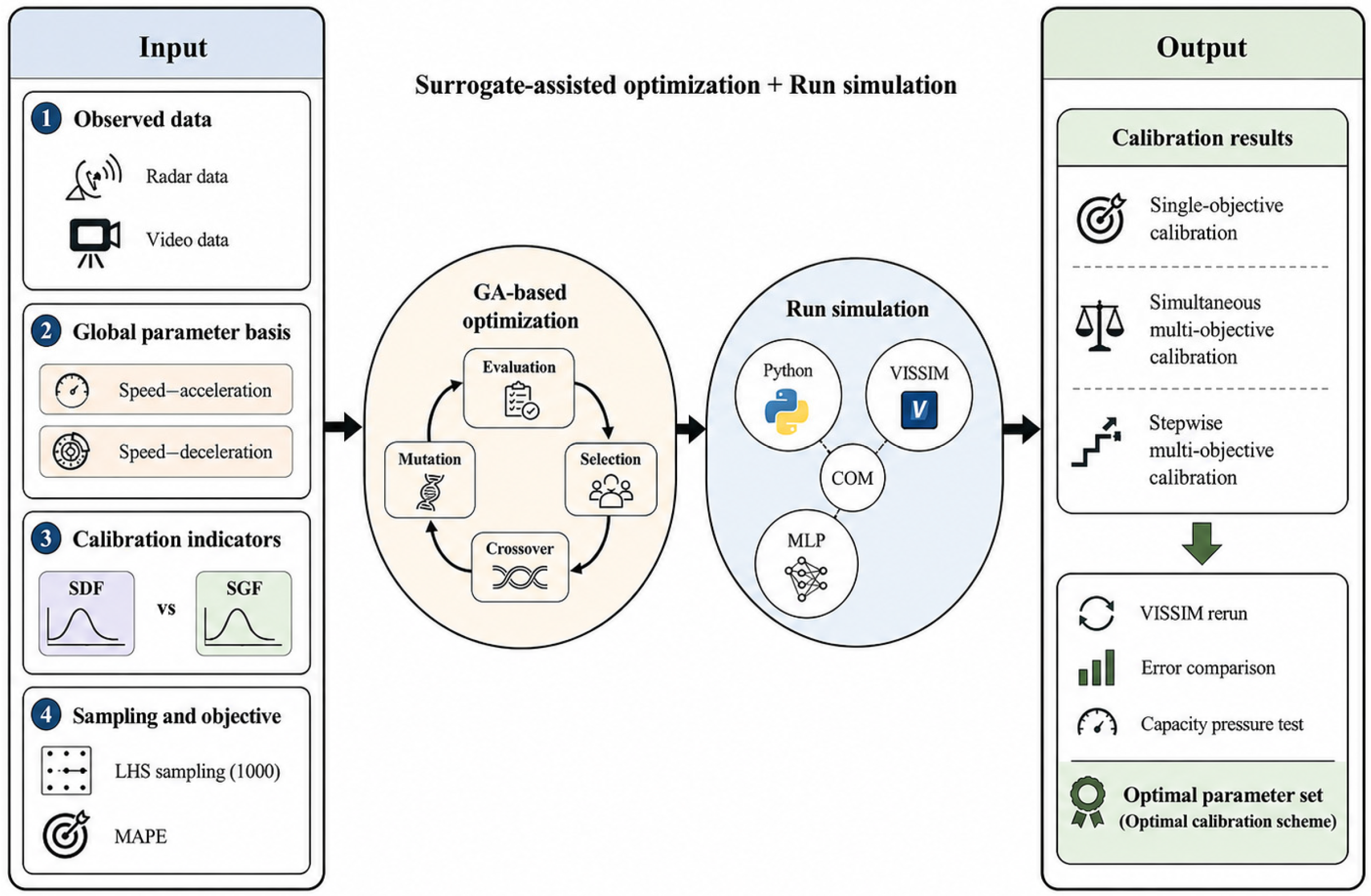
The methodological framework is summarized in Figure 1 and consists of five interconnected components: field data preparation, hierarchical parameter configuration, macro- and mesoscopic indicator construction, surrogate-assisted optimization, and calibration result validation. Field radar and video data are first processed to establish the simulation inputs and the observed calibration targets. Global vehicle dynamics settings, including desired speed, acceleration, and deceleration characteristics, are determined from field observations before the local driving behavior parameters are optimized [11]. The SDF and SGF are then constructed to represent the macroscopic cumulative speed distribution and the mesoscopic speed–spacing relationship, respectively [7,17,19].

Latin Hypercube Sampling and VISSIM (PTV Planung Transport Verkehr GmbH, Karlsruhe, Germany) batch simulations are used to generate the parameter–indicator dataset, from which separate MLP surrogate models are developed for the SDF and SGF [30,32]. The surrogate models serve as efficient fitness evaluation tools during GA-based optimization rather than as the principal methodological contribution. Single-objective, simultaneous multi-objective, SGF-priority stepwise, and SDF-priority stepwise strategies are compared to examine how the ordering of macro- and mesoscopic constraints affects calibration performance. The resulting parameter sets are finally assessed through VISSIM reruns, repeated random seed tests, and an out-of-objective capacity pressure test. The following subsections describe each component and its implementation in detail.

2.1. Study Site and Data Preparation

The Shenzhen–Zhongshan Link tunnel section was selected as the study site. The field traffic data and the simulation scenario were both derived from this tunnel section. The tunnel is a bidirectional eight-lane facility with a design speed limit of 100 km/h and a total length of approximately 6.8 km. Its constrained geometric environment, stable lane-use rules, and traffic states ranging from free flow to high demand provide a representative continuous-flow tunnel setting for evaluating the proposed calibration framework.

Traffic operation differs across lane groups. The inner lanes are used predominantly by passenger cars and generally exhibit higher and more concentrated speeds, whereas the outer lanes carry mixed passenger car and truck traffic and are more strongly affected by heavy vehicle operations and continuous car-following interactions. Lane attributes and vehicle types were therefore retained during data processing and simulation-model development.

Two field data sources were used, as summarized in

Table 1. Field data sources and usage in model calibration.

Data Source	Collection Information	Main Data Content	Usage in This Study
Radar detection data	30 September to 14 October 2025; tunnel-wide detection	Vehicle speed and flow information	Constructing speed distribution samples and observed SDF curves
Fixed-point video data	Six key locations inside the tunnel; 48 h in total	Vehicle trajectories, vehicle types, passing times, and car-following states	Identifying car-following samples and extracting net spacing for observed SGF construction

. Radar data were collected from 30 September to 14 October 2025 and provided vehicle speed and traffic flow observations for constructing the observed SDF and configuring the traffic demand inputs. Fixed-point video data were collected at six representative locations inside the tunnel, with approximately 48 h of raw video available. A continuous peak-hour period with relatively high traffic volume and abundant car-following interactions was selected for detailed trajectory extraction. The selected 1 h video data were used to identify vehicle types, lane positions, passing times, leading–following relationships, and net spacing for SGF construction.

Data preprocessing was conducted separately for the radar and video datasets. Radar records containing abnormal or missing speed and flow values were removed. For the video data, trajectories affected by severe occlusion, unreliable vehicle classification, discontinuous tracking, or ambiguous leading–following relationships were excluded. The retained observations were classified by lane and vehicle type. The processed radar data formed the speed distribution dataset, whereas the valid trajectory pairs extracted from the selected video period formed the car-following dataset.

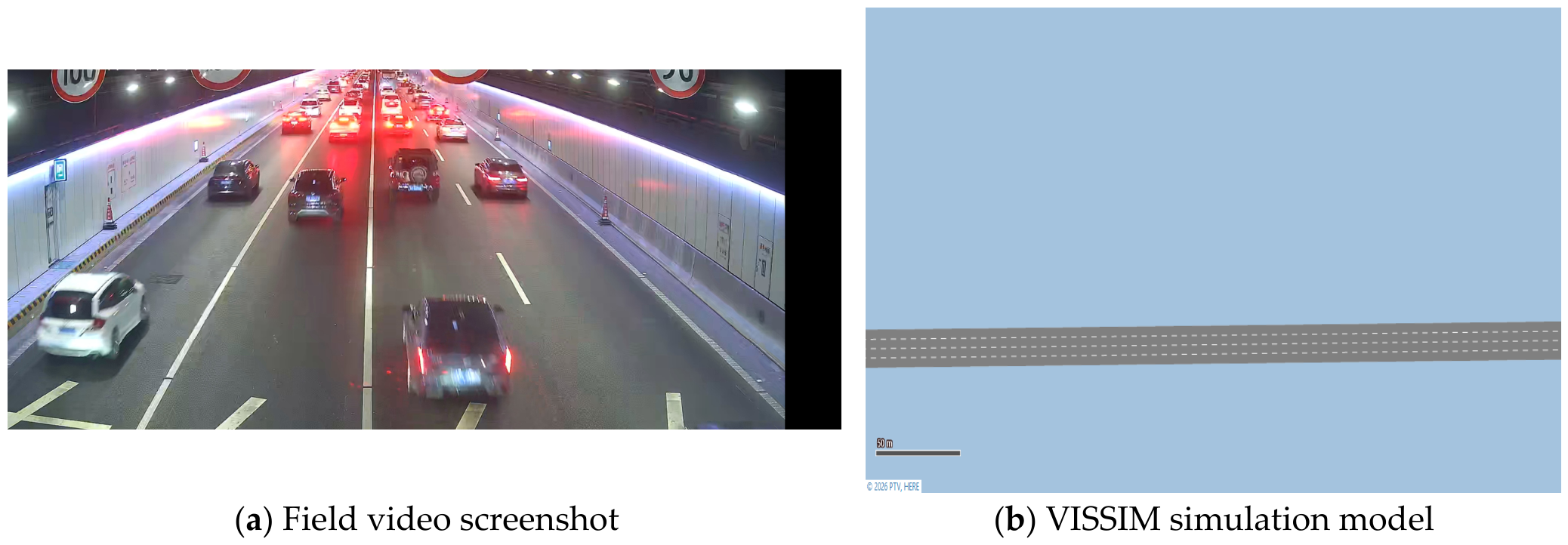
A VISSIM model corresponding to the study section was then constructed using the observed tunnel geometry, lane-use rules, traffic demand, vehicle composition, and vehicle dynamics characteristics. These external conditions were kept consistent across the calibration strategies so that differences in model performance could be attributed to the calibration method and parameter solutions rather than to changes in the simulation scenario. The field video view and the corresponding VISSIM model are shown in Figure 2.

2.2. Multi-Level Parameter System

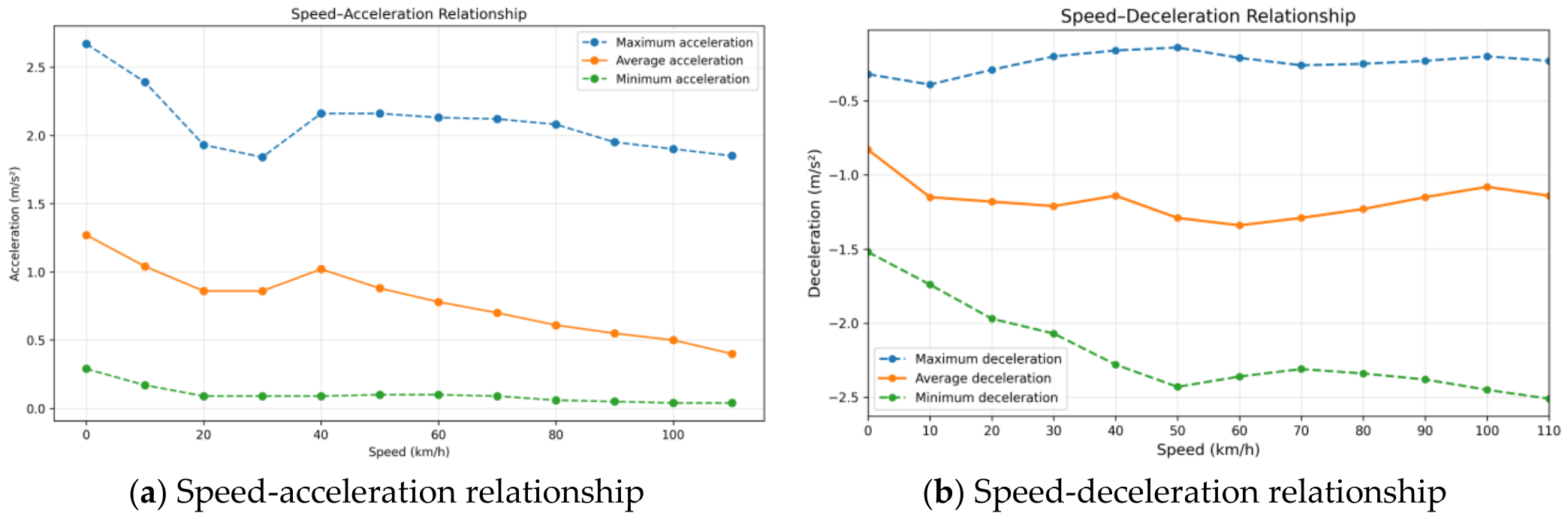
To improve the physical interpretability of the calibration results, the parameters of the VISSIM microscopic traffic simulation model were organized into a multi-level parameter system. In this study, the parameters were divided into global vehicle dynamics parameters and local driving behavior parameters. The global parameters describe the basic motion capability of vehicles, including desired speed, acceleration, and deceleration characteristics. These parameters were configured first using field data from the Shenzhen–Zhongshan Link tunnel. Specifically, the speed distribution characteristics of different vehicle types under free-flow conditions were extracted, and the observed speed–acceleration and speed–deceleration relationships were used to determine the corresponding vehicle dynamic settings in VISSIM, as shown in Figure 3.

A total of 19 local driving behavior parameters were jointly calibrated. These included all ten Wiedemann 99 car-following parameters, CC0–CC9, which describe desired spacing, speed difference perception, following state transitions, oscillation, and acceleration responses. Two additional parameters, OB_d and N_pr, represent the longitudinal perception distance and the number of preceding vehicles considered by the driver. The remaining seven parameters—ACC_max, ACC_ac, D, T_dis, GAP_min, ABX, and CO_ac—describe lane-changing gap acceptance, waiting behavior, safety distance adjustment, and cooperative deceleration.

All 19 parameters were retained in the calibration rather than being reduced through preliminary parameter screening. This design was adopted because parameters associated with car-following, anticipation, and lane-changing interactions may jointly influence both the mesoscopic SGF and the macroscopic SDF. Excluding individual parameters before optimization could restrict the feasible solution space or cause their effects to be indirectly absorbed by other parameters. The same parameter set and value ranges were therefore used for all calibration strategies to ensure a consistent comparison. The definitions and calibration ranges of the selected parameters are presented in

Table 2. Calibration parameters and value ranges.

Parameter	Description	Value Range
CC0	Standstill distance, indicating the minimum desired spacing between vehicles when stationary	(0.5, 3.0)
CC1	Desired time headway, representing the speed-dependent safety spacing time that drivers intend to maintain during driving	(0.5, 3.0)
CC2	Following variation range, indicating the additional distance allowed beyond the desired safety distance during car-following	(1.5, 10.0)
CC3	Threshold for entering the following state, representing the time threshold before a vehicle starts decelerating when approaching a slower leading vehicle	(−15, −4)
CC4	Negative speed difference threshold, indicating the lower threshold for the following vehicle’s deceleration response relative to the leading vehicle	(−2.0, −0.1)
CC5	Positive speed difference threshold, indicating the upper threshold for the following vehicle’s acceleration response relative to the leading vehicle	(0.1, 2.0)
CC6	Influence coefficient of distance on speed oscillation, reflecting the effect of following distance variation on speed fluctuation	(2, 20)
CC7	Following oscillation acceleration, representing the acceleration amplitude associated with speed oscillation in the following state	(0.1, 0.6)
CC8	Standstill acceleration, representing the desired acceleration when a vehicle starts from rest	(1.0, 4.0)
CC9	High-speed acceleration, representing the desired acceleration under relatively high-speed conditions	(0.5, 3.0)
OB_d	Longitudinal perception distance, indicating the range within which a vehicle can perceive vehicles ahead and respond to the traffic state	(150, 350)
N_pr	Number of preceding vehicles perceived and considered by the driver, affecting the driver’s anticipation of the downstream traffic state	(1, 5)
ACC_max	Maximum acceptable deceleration during lane changing, reflecting the risk tolerance of the lane-changing process	(−6, −2)
ACC_ac	Acceptable deceleration during lane changing, which affects the gap acceptance behavior in the target lane	(−2,−0.5)
D	Distance parameter for maintaining a stable spacing with vehicles in the target lane during lane changing	(50, 250)
T_dis	Maximum waiting time tolerated by the driver after deciding to change lanes	(10, 60)
GAP_min	Minimum safety gap required for lane changing, reflecting the minimum lane-changing gap under low-speed or stopped conditions	(0.5, 5.0)
ABX	Safety distance reduction factor, reflecting the driver’s acceptance of reduced safety spacing during lane-changing interactions	(0.1, 1.0)
CO_ac	Cooperative deceleration, indicating the acceptable deceleration of vehicles in the target lane to allow a lane-changing vehicle to enter	(−5, −1)

.

2.3. Macro- and Mesoscopic Calibration Indicators

To constrain the simulation model from both operational and behavioral perspectives, this study constructs two calibration indicators: the SDF and SGF. The SDF is used as a macroscopic indicator to describe the overall speed distribution of tunnel traffic, while the SGF is used as a mesoscopic indicator to characterize the relationship between vehicle speed and net spacing under car-following conditions. The combination of these two indicators allows the calibration process to evaluate not only whether the simulated traffic state is consistent with field observations, but also whether the simulated car-following behavior is behaviorally reasonable.

2.3.1. Speed Distribution Function

The SDF was constructed based on vehicle operating speed. Because instantaneous speed observations may be affected by short-term fluctuations and detection noise, the average speed of each vehicle over a continuous 5 s period was used as its representative operating speed. Let the 5 s average speed of vehicle $i$ be denoted as ${\overline{v}}_i$, the speed threshold as $s_k$, and the total number of vehicle samples as $\mathrm{N}$. The proportion of vehicles with speeds not exceeding the threshold $s_k$ can then be calculated using Equation (1).

$$F_v(s_k)={\displaystyle \frac{1}{N}}{\displaystyle \sum _{i=1}^{N}I({\overline{v}}_i\le s_k)}$$

(1)

where $F_v(s_k)$ is the cumulative Speed Distribution Function, and I(∙) is an indicator function that equals 1 when the specified condition is satisfied and 0 otherwise.

The speed thresholds ranged from 70 to 110 km/h at intervals of 5 km/h. The cumulative proportions corresponding to the same threshold sequence were calculated for both the field and simulated datasets, thereby producing the observed and simulated SDF curves. Compared with a single average speed value, the SDF retains information on the proportions of vehicles operating within different speed ranges and therefore provides a more comprehensive constraint on the macroscopic traffic state.

2.3.2. Speed Gap Function

The SGF was constructed to describe car-following behavior under continuous-flow conditions. It does not represent a new car-following law; rather, it reformulates the established speed–spacing relationship as a curve-based mesoscopic calibration indicator.

Car-following samples were identified from both field trajectories and VISSIM trajectory outputs. A sample was considered valid when: (1) the leading and following vehicles travelled in the same lane and direction; (2) no other vehicle was located between them; (3) the leading–following relationship could be continuously and reliably identified; and (4) the net spacing was less than 200 m. The 200 m criterion was used as an upper screening boundary for candidate leading–following pairs rather than as an indication that all retained observations represented close-following conditions. This relatively broad upper limit avoided truncating the observed high-speed spacing distribution, in which mean net spacing exceeded 100 m in some speed intervals. Net spacing was defined as the front-to-front longitudinal distance between two consecutive vehicles minus the length of the leading vehicle.

Let the speed of sample $i$ be denoted as $v_i$, and the corresponding net spacing as $g_i$. To construct the SGF, the vehicle speed is discretized into several speed intervals, and the average net spacing of the samples within each interval is calculated:

$${\overline{g}}_i={\displaystyle \frac{1}{n}}{\displaystyle \sum _{i=1}^{n_j}{g}_i}$$

(2)

where ${\overline{g}}_i$ denotes the average net spacing corresponding to the j-th speed interval, and $n_j$ is the number of samples in that interval. By calculating the average net spacing for each speed interval under both observed and simulated conditions, the observed and simulated SGF curves can be obtained.

2.4. Simulation Sampling and Surrogate Model Development

Separate multilayer perceptron (MLP) surrogate models were developed for the SDF and SGF to reduce the computational cost of repeatedly evaluating candidate parameter combinations in VISSIM [30,32]. The input of each surrogate model consisted of the 19 local driving behavior parameters listed in Table 2, while the output consisted of the corresponding SDF or SGF curve values. The surrogate models were used as efficient fitness evaluation tools during the subsequent optimization procedure, whereas the final parameter solutions were still verified in the original VISSIM environment.

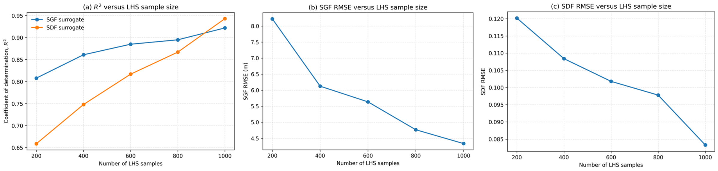
Latin Hypercube Sampling was used to generate 1000 parameter combinations within the prescribed parameter ranges. To examine whether the selected sample size was adequate for surrogate model development, five candidate sample sizes—200, 400, 600, 800, and 1000—were evaluated using consistent data-processing, dataset-partitioning, and network-training settings. The predictive performance at each sample size was assessed using the coefficient of determination ((R²)) and root mean square error (RMSE). The corresponding sample size convergence results are presented in Section 3.1.

Each sampled parameter combination was evaluated through VISSIM batch simulation using the COM interface. Each simulation lasted 4200 s, including a 600 s warm-up period that was excluded from indicator calculation. To reduce stochastic variation in the simulation-generated training targets, every parameter combination was simulated using five random seeds: 20, 30, 40, 50, and 60. The SDF and SGF curves were calculated separately for each run, and the mean curve values across the five seeds were used as the outputs associated with that parameter combination.

Vehicle operation and trajectory data were extracted from the VISSIM output files after each run. The same vehicle filtering, car-following identification, speed interval division, and indicator calculation procedures described in Section 2.3 were applied to both the field and simulated data. A parameter–indicator dataset containing 1000 input–output samples was thereby constructed for surrogate model training and evaluation.

Because the SDF and SGF differ in their output dimensions and nonlinear response characteristics, their surrogate models were trained separately. Before training, both the input parameters and output indicators were standardized. The dataset was randomly divided into training, validation, and test subsets at a ratio of 7:2:1. The training subset was used to estimate the network weights, the validation subset was used for model selection and early stopping, and the independent test subset was reserved for the final evaluation of predictive performance on previously unseen parameter combinations.

The rectified linear unit (ReLU) was adopted as the activation function, and the Adam algorithm was used for network optimization. The mean squared error (MSE) was used as the training loss function. The initial learning rate was set to 0.001, and the maximum number of training epochs was 200. The batch size followed the scikit-learn “auto” setting and therefore did not exceed 200 training samples. Early stopping was applied with a patience of 20 epochs, and training was terminated when the validation performance did not improve for 20 consecutive epochs.

Five candidate hidden-layer configurations were evaluated: (64), (64, 32), (128, 64, 32), (128, 64), and (256, 128). The final structures were selected according to their validation set performance. Predictive accuracy was then evaluated on the independent test set using MAPE, RMSE, and (R^2) after transforming the model outputs back to their original scales. In addition, the residuals were defined as the difference between the surrogate-predicted and VISSIM-generated values and were examined to identify possible systematic overestimation, underestimation, or heteroscedasticity. The network structure comparison, sample size convergence, test set accuracy, and residual distribution results are reported in Section 3.1.

During parameter optimization, the trained surrogate models predicted complete SDF or SGF curves for candidate parameter combinations. The corresponding calibration errors were then calculated and used as fitness values in the genetic algorithm. This surrogate-assisted procedure avoided repeated VISSIM execution within every optimization iteration; however, surrogate predictions were not treated as the final calibration results, and all selected parameter solutions were subsequently rerun and evaluated in VISSIM.

2.5. Calibration Objectives and Strategies

The Mean Absolute Percentage Error (MAPE) was used to measure the fitting error between simulated and observed indicators. For both the SDF and SGF, MAPE was adopted as the objective value for parameter optimization. It is defined as follows:

$$MAPE={\displaystyle \frac{1}{n}}{\displaystyle {\sum }_{i=1}^n\left|\frac{{\widehat{y}}_i-y_i}{y_i}\right|}\times 100\%$$

(3)

where $y_i$ denotes the observed value of the $\mathrm{i}$-th item, ${\widehat{y}}_i$ denotes the corresponding predicted value, and $\mathrm{n}$ is the output dimension of the model result.

2.5.1. Genetic Algorithm Settings

The genetic algorithm was initialized with a population of 100 randomly generated chromosomes, with each chromosome representing one combination of the 19 calibration parameters. The fitness of each chromosome was evaluated using the objective value calculated from the indicator curve predicted by the corresponding surrogate model.

At each generation, the chromosomes were ranked according to their objective values, and the 20 chromosomes with the lowest errors were retained as the parent pool. Fifty offspring were generated through crossover by randomly combining parameter values selected from the parent chromosomes. Another 50 offspring were generated through mutation. For the mutation operation, selected parameter values were perturbed within ±5% of their parent values and restricted to the original calibration ranges listed in Table 2.

The resulting 100 offspring formed the population of the next generation. The evaluation, selection, crossover, and mutation procedures were repeated for 50 generations. The same population size, parent selection rule, crossover procedure, mutation rule, and number of generations were applied to all calibration strategies to ensure a consistent comparison.

2.5.2. Single-Objective Calibration

For single-objective calibration, the SDF and SGF errors were minimized separately:

$$[\underset{\mathit{\theta }}{\min }{E}_{\mathrm{S}\mathrm{D}\mathrm{F}}(\mathit{\theta }),]$$

(4)

$$[\underset{\mathit{\theta }}{\min }{E}_{\mathrm{S}\mathrm{G}\mathrm{F}}(\mathit{\theta }).]$$

(5)

The resulting SDF-oriented and SGF-oriented parameter solutions were used to examine whether an indicator from only one traffic system level could adequately constrain the other indicator.

2.5.3. Simultaneous Multi-Objective Calibration

For simultaneous multi-objective calibration, the SDF and SGF were incorporated into one comprehensive objective function. Although both errors were expressed as MAPE, their distributions and variation ranges across the simulation samples were different. To prevent the indicator with the larger numerical variation from dominating the combined objective, the two errors were normalized using the minimum and maximum values obtained from the 1000 LHS samples:

$${\mathrm{E}}_{\mathrm{q}}^{\prime }(\mathit{\theta })={\displaystyle \frac{E_q\left(\mathit{\theta }\right)-E_q^{\mathrm{m}\mathrm{i}\mathrm{n}}}{E_q^{\mathrm{m}\mathrm{a}\mathrm{x}}-E_q^{\mathrm{m}\mathrm{i}\mathrm{n}}}},\hspace{1em}\hspace{1em}q\in \left\{\mathrm{S}\mathrm{D}\mathrm{F}, \mathrm{S}\mathrm{G}\mathrm{F}\right\},$$

(6)

where $E_q^{\mathrm{m}\mathrm{i}\mathrm{n}}$ and $E_q^{\mathrm{m}\mathrm{a}\mathrm{x}}$ are the minimum and maximum errors of indicator $\mathrm{q}$ obtained from the LHS sample set.

For the equal-weighted scheme, the normalized SDF and SGF errors were assigned equal weights:

$$J_{eq}\left(\mathit{\theta }\right)=0.5{E_{\mathrm{S}\mathrm{D}\mathrm{F}}}^{\prime }\left(\mathit{\theta }\right)+0.5{E_{\mathrm{S}\mathrm{G}\mathrm{F}}}^{\prime }\left(\mathit{\theta }\right)$$

(7)

.

For the entropy-weighted scheme, the weights were determined from the dispersion of the normalized errors within the LHS sample set. Let $z_{ij}$ denote the normalized error of sample $\mathrm{i}$ for indicator $\mathrm{j}$. Its proportion was calculated as:

$${\mathrm{p}}_{\mathrm{i}\mathrm{j}}={\displaystyle \frac{z_{ij}}{{\sum }_{i=1}^m{z}_{ij}}}$$

(8)

where $\mathrm{m}$ is the number of LHS samples. When $p_{ij}=0$, the term $p_{ij}\ln p_{ij}$ was defined as zero. The information entropy of indicator $\mathrm{j}$ was then calculated as:

$$e_j=-k{\displaystyle \sum _{i=1}^m{p}_{ij}\ln p_{ij}}$$

(9)

where $m$ is the number of samples and $k=1/\ln m$. The information utility coefficient for the j-th indicator can then be obtained as:

$$d_j=1-e_j$$

(10)

The weight of the j-th indicator is determined as:

$$w_j={\displaystyle \frac{d_j}{{\sum }_{j=1}^2{d}_j}}$$

(11)

The entropy-weighted objective function was expressed as:

$${J_{ent}\left(\mathit{\theta }\right)=w}_{\mathrm{S}\mathrm{D}\mathrm{F}}{E_{\mathrm{S}\mathrm{D}\mathrm{F}}}^{\prime }\left(\mathit{\theta }\right)+w_{\mathrm{S}\mathrm{G}\mathrm{F}}{E_{\mathrm{S}\mathrm{G}\mathrm{F}}}^{\prime }\left(\mathit{\theta }\right),$$

(12)

where $w_{\mathrm{S}\mathrm{D}\mathrm{F}}+w_{\mathrm{S}\mathrm{G}\mathrm{F}}=1$. The equal-weighted and entropy-weighted schemes were used as simultaneous multi-objective benchmarks for comparison with the stepwise strategies.

2.5.4. Stepwise Macro- and Mesoscopic Calibration

The stepwise strategies optimized all 19 parameters in both stages rather than assigning predefined parameter subsets to individual indicators. In the first stage, the surrogate model corresponding to the priority indicator was combined with the genetic algorithm to search the full parameter ranges listed in Table 2.

After the first-stage optimal parameter vector ${\mathsf{\theta }}^{\mathrm{*}}$ was obtained, a local parameter region was constructed around this solution. For parameter $\mathrm{j}$, the second-stage lower and upper bounds were defined as:

$${\mathrm{L}}_{\mathrm{j}}^{\left(2\right)} = \max [L_j, \min (0.9{\mathsf{\theta }}_j^{*}, 1.1{\mathsf{\theta }}_j^{*}\left)\right]$$

(13)

$${\mathrm{U}}_{\mathrm{j}}^{\left(2\right)} = \min [U_j, \max (0.9{\mathsf{\theta }}_j^{*}, 1.1{\mathsf{\theta }}_j^{*}\left)\right]$$

(14)

where $L_j$ and $U_j$ are the original lower and upper bounds listed in Table 2, and $L_j^{\left(2\right)}$ and $U_j^{\left(2\right)}$ are the corresponding local bounds used in the second-stage optimization. The use of the minimum and maximum operators ensured correct bound definition for parameters with negative values.

A new population of 100 chromosomes was randomly generated within the resulting local parameter region. The surrogate model corresponding to the second indicator was then combined with the genetic algorithm to continue optimization. The same population size, parent selection rule, crossover procedure, mutation rule, and number of generations as those used in the first stage were applied.

In the SGF-priority stepwise strategy, the SGF surrogate model was first combined with the genetic algorithm to search the full parameter space and obtain the SGF-optimal parameter vector. A local search region of ±10% was then constructed around this solution. Within this restricted region, the SDF surrogate model was used to evaluate candidate parameter combinations, and the genetic algorithm minimized the SDF error.

Restricting the second-stage search to the neighborhood of the SGF-optimal solution limited large departures from the car-following characteristics established during the first stage, while allowing the macroscopic speed distribution to be further refined. The procedure did not strictly fix the first-stage parameter values or guarantee that the SGF error remained unchanged; instead, it reduced the possibility that the second-stage optimization would move to a substantially different region of the global parameter space.

The SDF-priority stepwise strategy followed the reverse procedure. The SDF surrogate model was first combined with the genetic algorithm to identify the SDF-optimal parameter vector over the full parameter space. A ±10% local region was subsequently constructed around this solution, and the SGF surrogate model was used to improve the speed–spacing relationship within the restricted parameter space.

The same neighborhood generation rule and genetic algorithm settings were applied to the SGF-priority and SDF-priority strategies to ensure comparability.

2.6. VISSIM Rerun and Stochastic Robustness Evaluation

The parameter solutions obtained through surrogate-assisted optimization were approximate optimal solutions evaluated by the MLP surrogate models. Therefore, the final parameter vectors obtained from the six calibration strategies were reintroduced into the original VISSIM model for simulation-based validation. No additional parameter optimization or local search was performed during this validation stage.

For each calibration strategy, the tunnel geometry, lane-use rules, traffic demand, vehicle composition, global vehicle dynamics settings, and simulation duration were kept unchanged. The SDF and SGF curves were recalculated from the VISSIM outputs using the same data-processing and indicator-construction procedures described in Section 2.3. Their MAPE values relative to the field-observed curves were then calculated using Equation (3). The VISSIM rerun results, rather than the surrogate model predictions, were used as the final calibration results reported in Section 3.

To evaluate whether the performance of the calibrated parameter sets was sensitive to simulation randomness, each calibration strategy was further tested using ten common random seeds: 2, 12, 22, 32, 42, 52, 62, 72, 82, and 92. The same seed sequence was applied to all six strategies so that their results could be compared under consistent stochastic simulation conditions.

For each random seed, the SGF MAPE and SDF MAPE were obtained from the rerun of the calibration scenario. The relative capacity deviation was obtained from the capacity pressure test described in Section 2.7. The distributions of these performance measures were summarized using boxplots, medians, and interquartile ranges.

Because the same random seeds were applied to all calibration strategies, the resulting observations formed paired samples. Given the limited number of random seed replications and without assuming normality, paired comparisons were conducted using the two-sided Wilcoxon signed-rank test. The SGF-priority stepwise strategy was treated as the reference scheme and was compared with each of the other five calibration strategies.

Holm correction was applied separately to the five comparisons conducted for each performance indicator to control the increase in Type I errors resulting from multiple comparisons. An adjusted p-value below 0.05 was considered statistically significant. For capacity performance, the signed relative deviation was retained in the boxplots to distinguish capacity overestimation from underestimation, whereas the absolute relative deviation was used in the statistical comparisons to represent capacity estimation accuracy.

2.7. Capacity Pressure Test

In addition to the SDF- and SGF-based calibration assessment, a capacity pressure test was conducted to evaluate the engineering applicability of the calibrated parameter sets. Capacity was not incorporated into the calibration objective functions. Therefore, the pressure test served as an out-of-objective engineering validation rather than as an additional calibration or parameter optimization step.

The pressure test was conducted over a total simulation duration of 2 h. The first 600 s were used as the warm-up period, during which the total entrance demand of the four lanes was set to 1200 pcu/h. Beginning at 600 s, the total entrance demand was increased by 1200 pcu/h every 600 s. During the test, the tunnel geometry, lane-use rules, observed vehicle composition, global vehicle dynamics settings, and calibrated local driving behavior parameters were kept unchanged.

For each demand-loading interval, the output flow, average speed, and operational stability of the tunnel section were recorded using a fixed-section detector. After vehicle counts were converted into passenger car equivalents, the highest stable 15 min output volume was multiplied by four to obtain the simulated hourly capacity. Similarly, the reference capacity was calculated by multiplying the highest observed 15 min passenger car-equivalent traffic volume extracted from the field video by four.

The pressure test was conducted for all six calibration strategies using the ten common random seeds specified in Section 2.6. One capacity value was obtained for each seed, and the arithmetic mean of the ten values was used as the representative capacity of each calibration strategy.

The relative capacity deviation was calculated as

$$D_C={\displaystyle \frac{C_{sim}-C_{ref}}{C_{ref}}}\times 100\%$$

(15)

where $C_{sim}$ is the simulated capacity obtained from the pressure test, $C_{ref}$ is the reference capacity of the study tunnel, and $D_C$ is the corresponding relative deviation.

A positive value of $D_C$ indicates that the simulated capacity was overestimated, whereas a negative value indicates that it was underestimated. The absolute value $\left|D_C\right|$ was used to evaluate the magnitude of the capacity estimation error in the statistical comparison.

The pressure test varied traffic demand while retaining the observed lane-use pattern and vehicle composition. It was intended to evaluate high-demand traffic flow performance rather than to provide a comprehensive sensitivity analysis of truck proportions, lane compositions, or geometric configurations.

3. Results

3.1. Surrogate Model Performance

The performance of the surrogate models was evaluated from four aspects: sample size adequacy, network structure selection, predictive accuracy on previously unseen parameter combinations, and residual characteristics.

First, the influence of the LHS sample size was examined using datasets containing 200, 400, 600, 800, and 1000 parameter combinations. Figure 4 shows the changes in (R²) and RMSE as the sample size increased. For the SDF surrogate model, (R²) increased from 0.659 at 200 samples to 0.817 at 600 samples and further increased to 0.943 at 1000 samples. Meanwhile, its RMSE decreased from 0.1202 to 0.1018 and finally to 0.0833. For the SGF surrogate model, (R²) increased from 0.808 at 200 samples to 0.885 at 600 samples and reached 0.922 at 1000 samples, while RMSE decreased from 8.224 m to 5.635 m and finally to 4.333 m.

These results indicate that the predictive performance of both surrogate models improved markedly as the sample size increased from 200 to 600. Further improvements were observed between 600 and 1000 samples, although the magnitude of improvement gradually decreased. Because the dataset containing 1000 parameter combinations provided the best overall predictive performance for both indicators, it was used for final surrogate model development.

Five candidate hidden-layer configurations were subsequently compared using the validation subset. As shown in

Table 3. Validation set MAPE of different MLP hidden-layer configurations.

MLP Network Structures	SGF MAPE (%)	SDF MAPE (%)
64	11.6	12.2
64-32	10.8	9.28
128-64-32	12.1	8.8
128-64	9.6	9.7
256-128	9.9	8.5

, the optimal network structure differed between the two calibration indicators. The structure with hidden layers of (128, 64) achieved the lowest validation MAPE for the SGF, whereas the structure of (256, 128) achieved the lowest validation MAPE for the SDF. These two configurations were therefore selected as the final SGF and SDF surrogate models, respectively.

The selected surrogate models were then evaluated using the independent test subset. The parameter combinations in this subset were not used for model training or network structure selection. As shown in

Table 4. Test set performance of the selected surrogate models.

Surrogate Model	MAPE (%)	RMSE	R2
SGF	9.8	4.333	0.922
SDF	8.3	0.083	0.943

, the selected SGF surrogate model achieves an R² of 0.922 and an RMSE of 4.333 m, while the selected SDF surrogate model achieves an R² of 0.943 and an RMSE of 0.083. The relatively high R² values and low prediction errors indicate that both models maintained acceptable predictive accuracy for previously unseen parameter combinations.

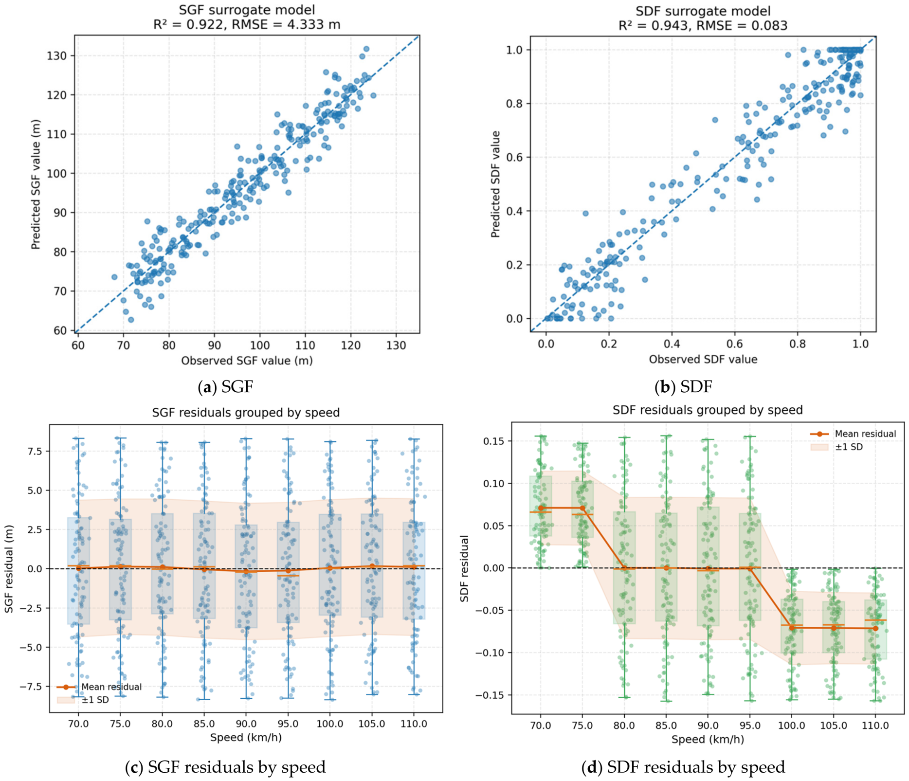
Figure 5 further illustrates the predictive and residual characteristics of the selected surrogate models on the independent test subset. As shown in Figure 5a,b, the surrogate-predicted values were generally distributed close to the 1:1 reference line for both the SGF and SDF, indicating good agreement with the corresponding VISSIM-generated values. For the SGF, the test set prediction achieved an R² of 0.922 and an RMSE of 4.333 m, while for the SDF, the corresponding values were 0.943 and 0.083.

Figure 5c,d present the residual characteristics across different speed intervals. For the SGF, the mean residuals at all speed intervals remained close to zero, indicating little systematic bias over the speed range. For the SDF, the mean residuals were close to zero over the middle speed range, whereas slight positive residuals were observed at lower speed thresholds and slight negative residuals at higher speed thresholds, indicating some local prediction bias across speed intervals. Nevertheless, the overall residual magnitudes remained limited, and the predictive accuracy was considered sufficient for using the surrogate models as efficient fitness evaluation tools during genetic algorithm optimization. The final calibration results were nevertheless determined from VISSIM reruns rather than from surrogate model predictions.

3.2. Single-Objective Calibration Results

Based on the trained surrogate models, parameter optimization was conducted using the SGF and SDF as separate objective functions. The resulting parameter sets were subsequently reintroduced into VISSIM, and the final indicator errors were calculated from the VISSIM rerun outputs. As shown in

Table 5. Optimal parameter sets obtained from the two single-objective calibration schemes.

Parameter	SDF Value	SGF Value
CC0	0.55	0.83
CC1	2.53	3.00
CC2	3.35	5.52
CC3	−6.94	−8.52
CC4	−0.97	−0.67
CC5	0.48	0.65
CC6	17.83	18.00
CC7	0.15	0.12
CC8	3.48	3.15
CC9	1.21	1.21
OB_d	174.30	260.51
N_pr	5.00	5.00
ACC_max	−3.97	−3.60
ACC_ac	−1.40	−1.30
D	162.40	220.25
T_dis	28.00	60.00
GAP_min	4.91	4.90
ABX	0.10	0.10
CO_ac	−3.06	−3.80

, the two single-objective schemes produced noticeably different parameter combinations, indicating that the SGF and SDF imposed different constraints on the parameter solution space.

The cross-indicator evaluation results are summarized in

Table 6. Cross-indicator performance of the single-objective calibration schemes.

	SGF MAPE (%)	SDF MAPE (%)
SGF single-objective calibration	11.84	13.78
SDF single-objective calibration	25.11	8.20

. The SGF single-objective scheme obtains an SGF MAPE of 11.84%, while its SDF MAPE increases to 13.78%. In contrast, the SDF single-objective scheme reduces the SDF MAPE to 8.20%, but its SGF MAPE increases to 25.11%. Thus, each scheme performed best for its own target indicator but showed weaker performance when evaluated using the other indicator.

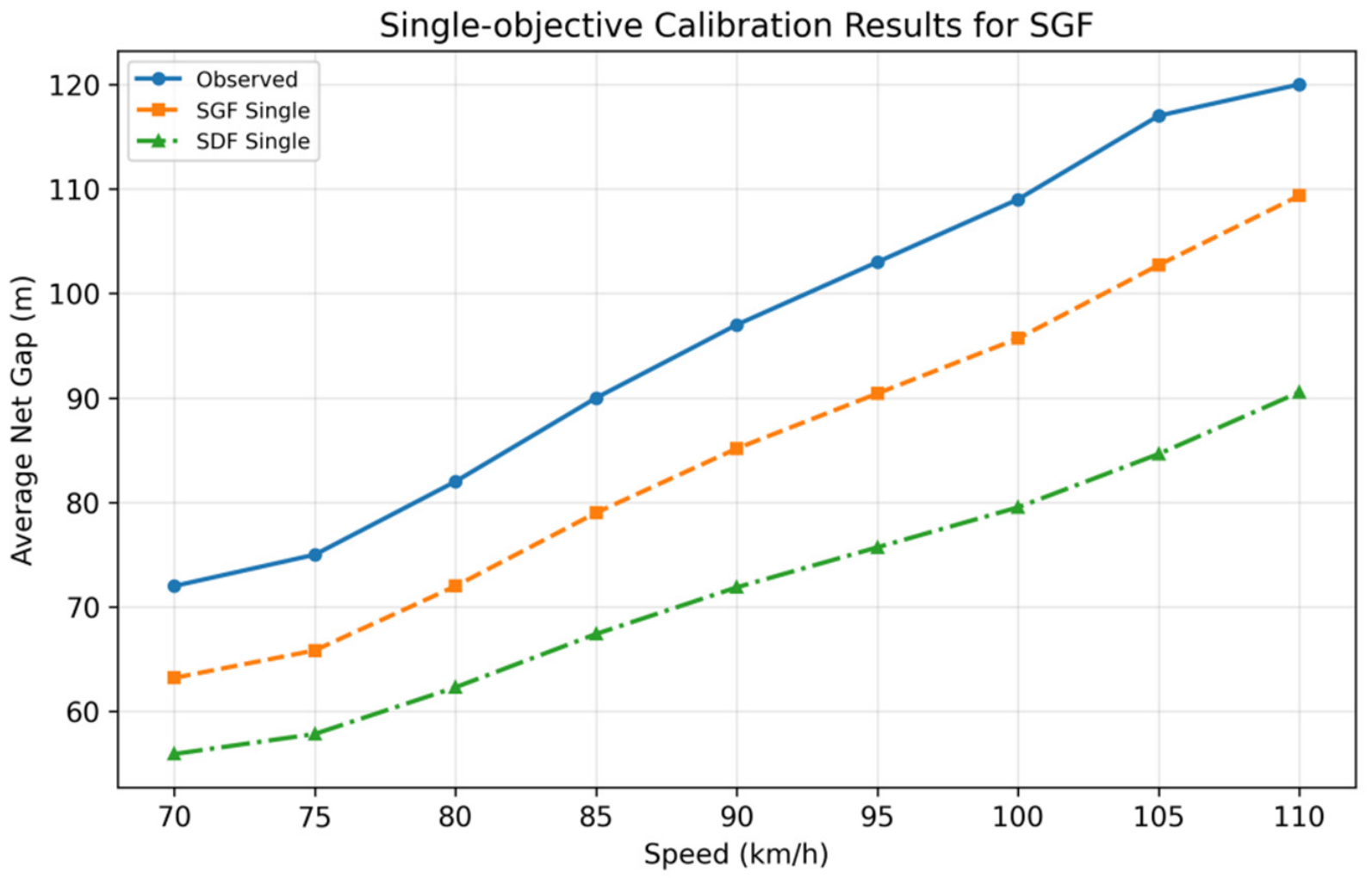
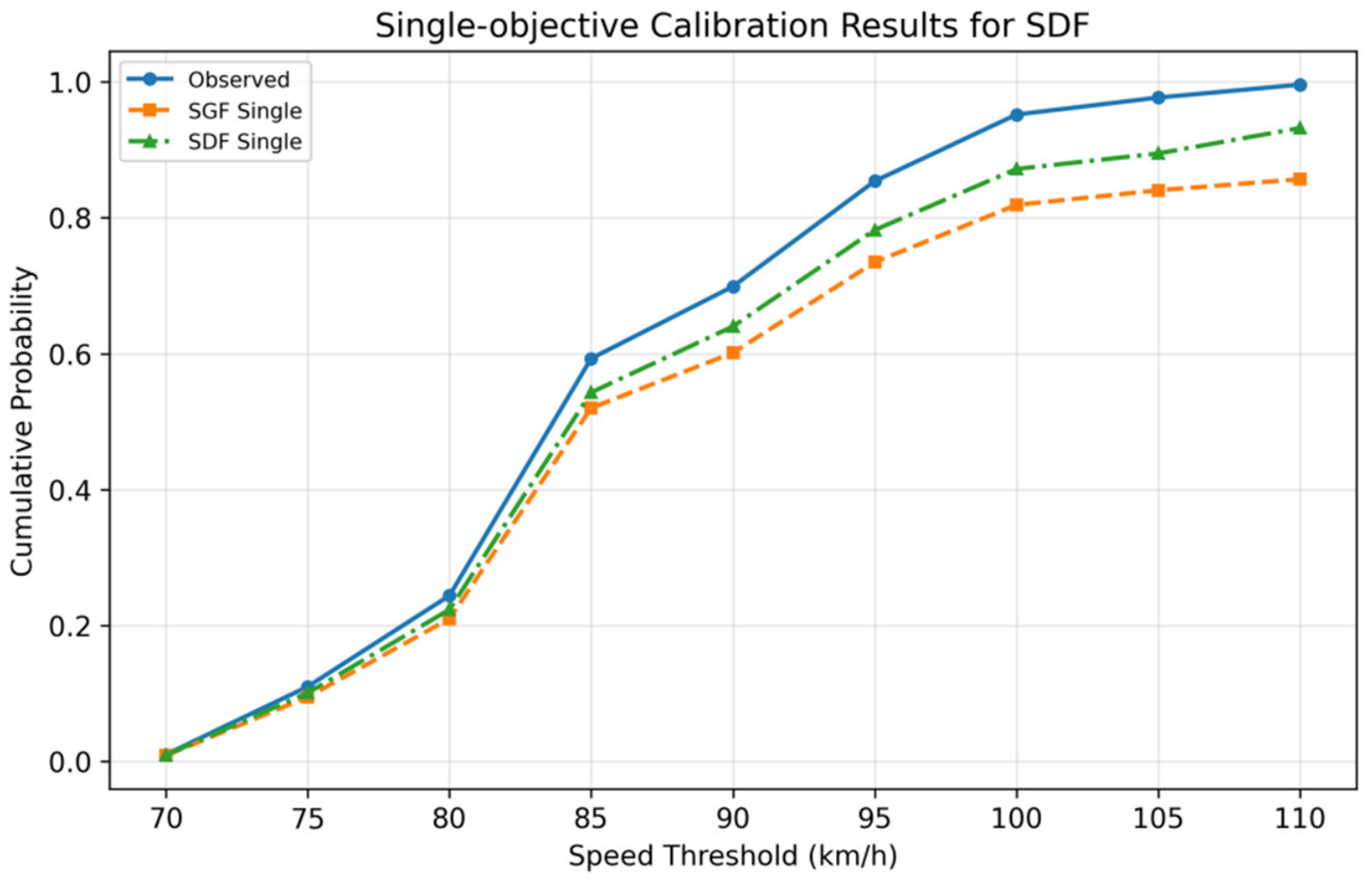
The curve comparisons in Figure 6 and Figure 7 further illustrate this indicator-specific behavior. In the SGF comparison, the SGF single-objective scheme followed the observed speed–spacing trend more closely, whereas the SDF single-objective scheme consistently underestimated the net spacing across the examined speed intervals. In the SDF comparison, the SDF single-objective scheme reproduced the observed cumulative speed distribution more closely, while the SGF single-objective scheme showed larger deviations, particularly at the higher speed thresholds.

Overall, the single-objective results show that calibration based on only one indicator leads to a clear indicator preference. SDF calibration reproduces the macroscopic speed distribution but does not adequately constrain the speed–spacing relationship, whereas SGF calibration better represents car-following behavior but provides a weaker constraint on the overall speed distribution. These results support the need to consider both indicators in the subsequent multi-objective calibration analysis.

3.3. Multi-Objective Calibration Results

The four multi-objective calibration strategies were evaluated using the SDF and SGF curves obtained from the final VISSIM reruns.

Table 7. Error summary of different multi-objective calibration strategies.

	SGF MAPE (%)	SDF MAPE (%)
SGF-priority stepwise calibration	12.00	11.53
SDF-priority stepwise calibration	27.32	8.61
Equal-weighted simultaneous calibration	12.96	13.79
Entropy-weighted simultaneous calibration	12.21	13.71

summarizes the SGF and SDF errors of the two simultaneous and two stepwise calibration strategies.

As shown in Table 7, the two simultaneous multi-objective strategies produced relatively similar results. The equal-weighted strategy obtained an SGF MAPE of 12.96% and an SDF MAPE of 13.79%, while the entropy-weighted strategy achieved an SGF MAPE of 12.21% and an SDF MAPE of 13.71%. These results indicate that both simultaneous strategies provided a compromise between the two calibration indicators.

The performance of the stepwise strategies differed clearly according to the calibration sequence. The SGF-priority strategy achieved an SGF MAPE of 12.00% and an SDF MAPE of 11.53%, showing relatively consistent performance across the two indicators.

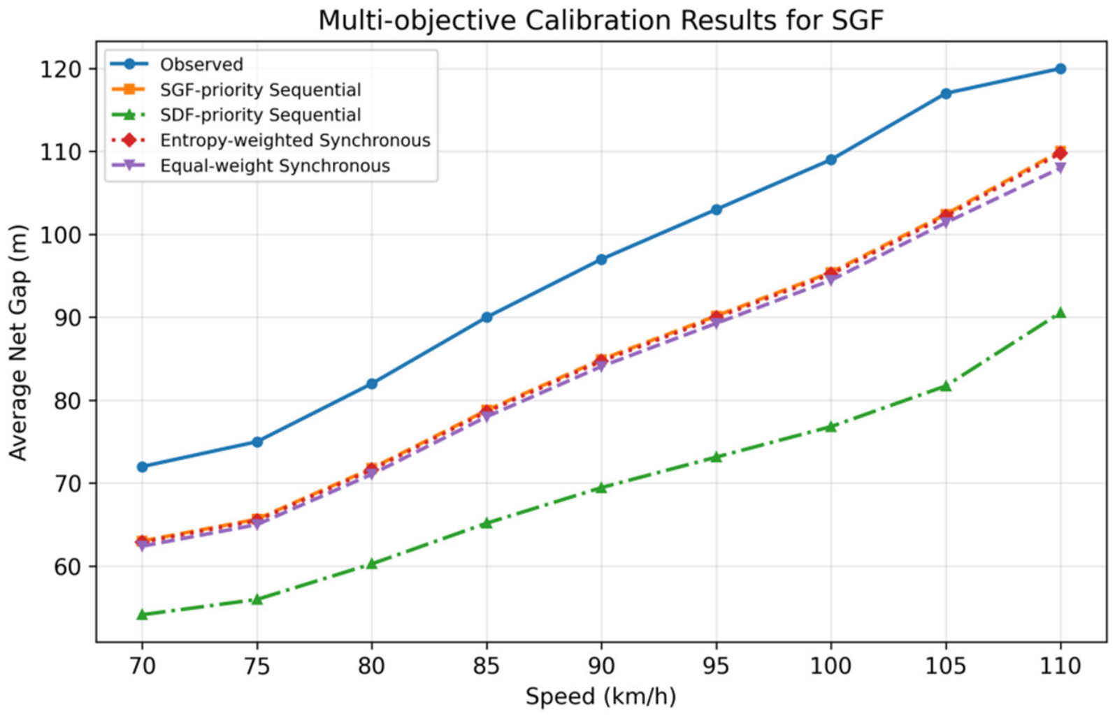
In contrast, the SDF-priority strategy achieved the lowest SDF MAPE of 8.61%, but its SGF MAPE increased markedly to 27.32%. This result indicates that prioritizing SDF produced a strong preference toward the macroscopic speed distribution indicator and did not provide comparable performance for the mesoscopic speed–spacing relationship.

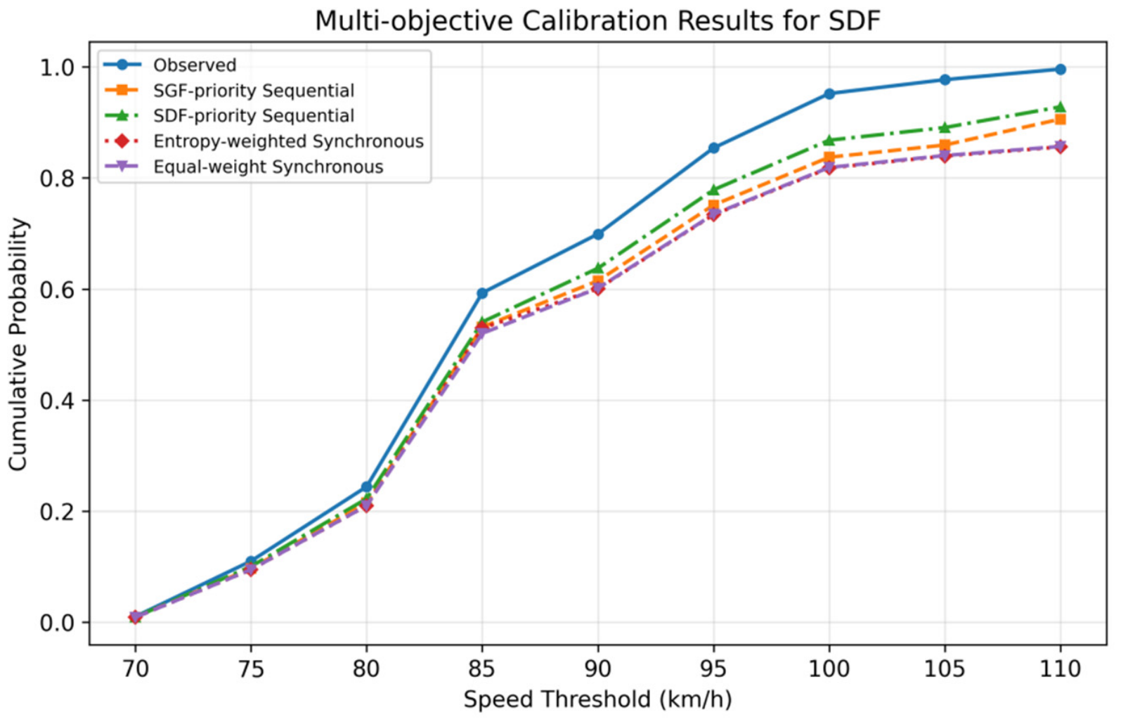
The curve comparisons in Figure 8 and Figure 9 are consistent with the numerical results. In Figure 8, the SGF-priority, equal-weighted, and entropy-weighted strategies show similar SGF trends, whereas the SDF-priority strategy consistently underestimates the observed net spacing. In Figure 9, the SDF-priority strategy follows the observed cumulative speed distribution most closely, while the SGF-priority strategy also maintains a reasonable fit across the examined speed thresholds.

Overall, the SGF-priority stepwise strategy provided the most consistent point estimate performance across the SGF and SDF among the four multi-objective strategies. The statistical robustness of these differences under common random seed conditions is further examined in Section 3.4.

3.4. Stochastic Robustness and Statistical Comparison

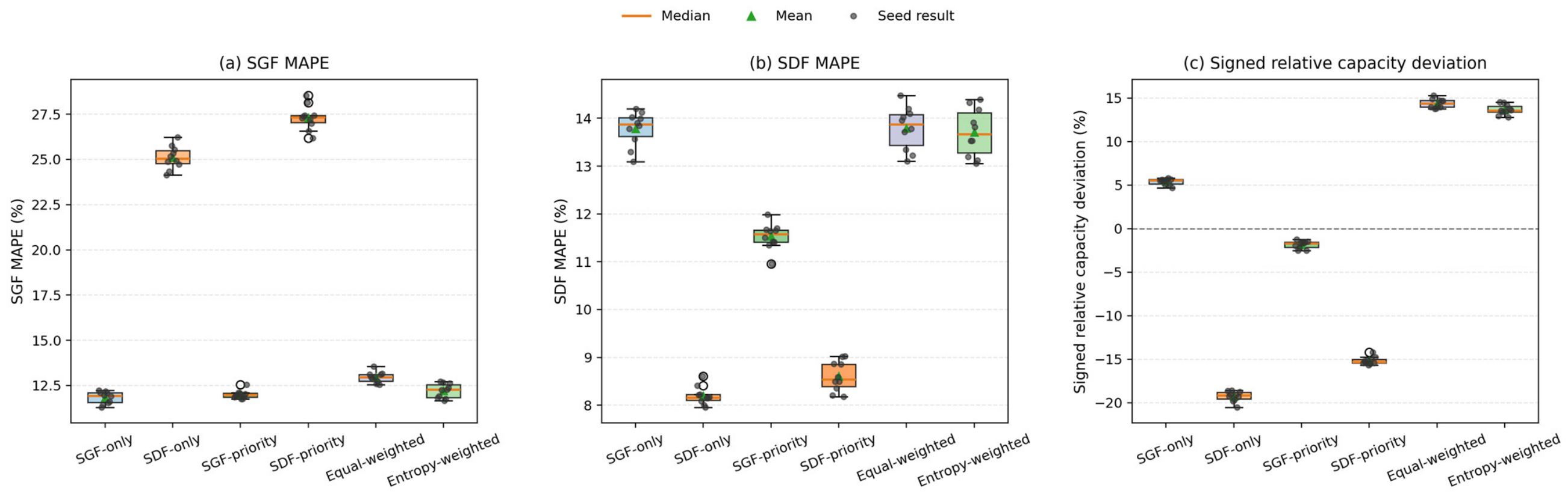
The stochastic robustness of the six calibration strategies was evaluated using the ten common random seeds specified in Section 2.6. Figure 10 presents the distributions of the SGF MAPE, SDF MAPE, and signed relative capacity deviation. The paired Wilcoxon signed-rank test results with Holm correction for comparisons between the SGF-priority strategy and the five benchmark strategies are summarized in

Table 8. Wilcoxon signed-rank test results with Holm correction for comparisons between the SGF-priority strategy and the benchmark strategies.

Performance Indicator	Comparison Strategy	Holm-Adjusted p-Value	Median Paired Difference (Percentage Points)	SGF-Priority Result
SGF MAPE	SGF-only	0.322	0.033	Higher
	SDF-only	0.010	−13.062	Lower
	SDF-priority	0.010	−15.361	Lower
	Equal-weighted	0.010	−0.993	Lower
	Entropy-weighted	0.211	−0.294	Lower
SDF MAPE	SGF-only	0.010	−2.302	Lower
	SDF-only	0.010	3.415	Higher
	SDF-priority	0.010	3.032	Higher
	Equal-weighted	0.010	−2.296	Lower
	Entropy-weighted	0.010	−2.099	Lower
Absolute capacity deviation	SGF-only	0.010	−3.866	Lower
	SDF-only	0.010	−17.477	Lower
	SDF-priority	0.010	−13.641	Lower
	Equal-weighted	0.010	−12.677	Lower
	Entropy-weighted	0.010	−11.886	Lower

. The relatively compact distributions within each calibration strategy indicate that the differences among the strategies were generally larger than the variations caused by the simulation random seeds.

For the SGF MAPE, the SGF-priority strategy showed a distribution close to those of the SGF-only and entropy-weighted strategies. The paired Wilcoxon tests confirmed that the differences between the SGF-priority and SGF-only $p_{\mathrm{a}\mathrm{d}\mathrm{j}}=0.322$ and between the SGF-priority and entropy-weighted calibration $p_{\mathrm{a}\mathrm{d}\mathrm{j}}=0.211$ were not statistically significant. In contrast, the SGF-priority strategy achieved significantly lower SGF errors than the SDF-only, SDF-priority, and equal-weighted strategies, with Holm-adjusted (p)-values of 0.010.

For the SDF MAPE, the SGF-priority strategy achieved significantly lower errors than the SGF-only, equal-weighted, and entropy-weighted strategies. However, its SDF error was significantly higher than those of the SDF-only and SDF-priority strategies. The adjusted (p)-values for all five comparisons were 0.010. These results show that the SGF-priority strategy was not the best scheme for the SDF indicator alone, but maintained a substantially lower SDF error than the strategies that did not prioritize the SDF.

For capacity performance, the boxplots retained the signed relative deviation to distinguish overestimation from underestimation, whereas the statistical tests used the absolute capacity deviation. The SGF-priority strategy achieved significantly smaller absolute capacity deviations than all five comparison strategies, with Holm-adjusted $p$-values of 0.010. This result indicates that its capacity-estimation advantage was consistently observed across the ten random seeds rather than being caused by a single simulation realization.

Overall, the repeated-seed analysis confirms that the SGF-priority strategy provides robust and balanced performance across the SGF, SDF, and capacity estimation. Its principal advantage is not achieving the minimum error for every individual indicator, but avoiding large deterioration in either calibration indicator while producing the smallest capacity estimation error.

3.5. External Validation by Capacity Pressure Test

The calibrated parameter sets were further evaluated through the capacity pressure test described in Section 2.7. The observed reference capacity was 6060.10 pcu/h, which was obtained by converting the highest observed 15 min passenger car-equivalent traffic volume to an hourly value. For each calibration strategy, the reported simulated capacity represents the arithmetic mean of the results obtained from the ten common random seeds.

As shown in

Table 9. Pressure test results of different calibration schemes.

Calibration Scheme	Capacity, S (pcu/h)	Relative Deviation (%)
SGF single-objective calibration	6387.35	5.40
SDF single-objective calibration	4892.93	−19.26
SGF-priority stepwise calibration	5948.59	−1.84
SDF-priority stepwise calibration	5140.14	−15.18
Equal-weighted simultaneous calibration	6931.52	14.38
Entropy-weighted simultaneous calibration	6888.10	13.66
Extracted reference value	6060.10	0.00

, the SGF-priority stepwise strategy produced a simulated capacity of 5948.59 pcu/h, corresponding to a signed relative deviation of −1.84% from the observed reference value. This was the smallest capacity deviation among the six calibration strategies.

The SGF-only strategy slightly overestimated the reference capacity by 5.40%. By contrast, the SDF-only and SDF-priority strategies underestimated capacity by 19.26% and 15.18%, respectively. The two simultaneous multi-objective strategies both overestimated capacity, with deviations of 14.38% for the equal-weighted strategy and 13.66% for the entropy-weighted strategy.

These results are consistent with the repeated-seed analysis in Section 3.4, in which the SGF-priority strategy achieved significantly smaller absolute capacity deviations than all five comparison strategies. Therefore, although the SGF-priority strategy did not minimize every individual calibration error, it provided the closest reproduction of the observed capacity while maintaining relatively consistent SGF and SDF performance.

4. Discussion

4.1. Effect of Calibration Sequence

The results indicate that the order of macro- and mesoscopic calibration affects the behavioral meaning of the final parameter solution. The SDF describes the aggregate speed distribution, whereas the SGF represents the speed–spacing relationship under car-following conditions. Similar SDF curves may be produced by different combinations of car-following and lane-changing parameters; therefore, good SDF fitting does not necessarily ensure realistic vehicle interactions.

In the SGF-priority strategy, the first stage restricts the solution to a parameter region that reproduces the observed car-following relationship. The SDF is then refined within a local neighborhood, limiting large departures from the established behavioral pattern. In contrast, when the SDF is optimized first, the resulting region may already contain behaviorally inconsistent parameter combinations, and the restricted second stage may not fully correct the SGF deviation. This explains why the mesoscopic-to-macroscopic sequence provides a more balanced result.

The simultaneous schemes consider both indicators but allow improvement in one objective to compensate for deterioration in the other. Equal weighting produces a numerical compromise, while entropy weighting changes the relative importance of the indicators according to their dispersion. Neither approach explicitly establishes behavioral consistency before macroscopic adjustment. The contribution of the proposed method therefore lies in the calibration sequence rather than simply combining two objectives.

4.2. Behavioral and Capacity Interpretation

The parameter differences between the SDF- and SGF-oriented solutions further illustrate the limitations of calibration based only on aggregate traffic states. Parameters such as CC1, CC2, OB_d, and D are related to desired headway, spacing variation, forward perception, and lane-changing interaction distance. Their differences suggest that similar speed distributions can be generated by parameter sets with different vehicle-interaction characteristics. These observations provide behavioral interpretation, but they should not be regarded as a formal parameter sensitivity ranking.

The capacity pressure test provides additional evidence. Capacity is influenced by effective spacing, response to speed differences, acceleration recovery, and lane-changing interactions. Consequently, a parameter set may reproduce the observed speed distribution but still produce unrealistic discharge flow under increasing demand. The lower capacities obtained from the SDF-oriented schemes may reflect overly restrictive or unstable interactions, whereas the higher capacities of the simultaneous schemes may result from overly efficient spacing or gap acceptance behavior. The SGF-priority strategy reduces both types of deviation by first constraining longitudinal interaction behavior and then correcting the macroscopic speed state.

4.3. Methodological and Practical Implications

Previous ANN-assisted calibration studies have primarily used neural networks or other surrogate models to approximate parameter–output relationships and reduce the computational burden of repeated microsimulation evaluations [30,31,32]. The present study uses the MLP surrogate models in a similar computational role to support genetic-algorithm optimization. However, the surrogate model architecture itself is not the principal methodological contribution. Compared with ANN-assisted approaches that primarily emphasize prediction accuracy or optimization efficiency, the proposed framework focuses on the ordered coordination of calibration constraints: the SGF first restricts the parameter space according to the observed speed–spacing relationship, and the SDF subsequently refines the macroscopic speed distribution within the resulting local region. Therefore, the methodological novelty lies in the stepwise macro- and mesoscopic calibration sequence rather than in the use of an ANN surrogate model alone.

For practical application, the framework provides a more behaviorally constrained simulation model for tunnel operation analysis, management strategy evaluation, and capacity assessment. It reduces the risk that a model fits observed speeds through unrealistic parameter compensation. The approach is particularly suitable for facilities where radar data can provide continuous speed observations and video data can support car-following identification.

4.4. Limitations and Future Research

This study is based on one continuous-flow tunnel and one simulation platform. The results may therefore depend on the tunnel geometry, speed limit, vehicle composition, lane-use pattern, and Wiedemann 99 model. In addition, the SGF construction requires reliable vehicle trajectories and leading–following identification, which may be affected by occlusion and detection errors.

The pressure test varied traffic demand while keeping vehicle composition and lane-use rules unchanged. It should therefore be regarded as an out-of-objective engineering validation rather than a comprehensive sensitivity analysis. In addition, a systematic global sensitivity analysis of the 19 calibrated parameters was not conducted. Consequently, the parameter differences observed among the calibration strategies should be interpreted as behavioral contrasts between alternative solutions rather than as a formal ranking of parameter importance. The ±10% neighborhood used in the second calibration stage was also fixed rather than independently optimized. Future research should examine parameter sensitivity and interactions, evaluate alternative neighborhood widths, and further test the proposed calibration sequence across different tunnels, freeway facilities, mixed-traffic conditions, and simulation platforms.

5. Conclusions

This study developed a stepwise macro- and mesoscopic calibration framework for microscopic traffic simulation in continuous-flow tunnel environments. The principal contribution is the integration of a macroscopic traffic state indicator and a mesoscopic car-following indicator within a hierarchical optimization process. The SDF describes the cumulative speed distribution, whereas the SGF constrains the speed-dependent net-spacing relationship. MLP surrogate models improve optimization efficiency, but the methodological novelty lies in using the SGF to establish a behaviorally plausible parameter region before refining the macroscopic traffic state with the SDF.

The comparison among single-objective, simultaneous, and stepwise strategies shows that accurate reproduction of one traffic level does not guarantee consistency at another. Macroscopic speed calibration alone permits behaviorally different parameter combinations to produce similar aggregate results, while simultaneous weighting may yield a compromise without preventing cross-indicator compensation. Prioritizing the SGF provides a more physically interpretable sequence because longitudinal vehicle interactions form the behavioral basis from which aggregate traffic states emerge. The subsequent SDF stage can improve macroscopic consistency while limiting large departures from the established car-following pattern.

The out-of-objective capacity pressure test further indicates that behavioral consistency is relevant to engineering performance. A parameter set that reproduces observed speeds but misrepresents vehicle spacing and interaction dynamics may produce biased capacity estimates under increasing demand. By balancing the speed–spacing relationship and speed distribution, the proposed framework provides a more credible basis for tunnel traffic operation analysis, traffic management strategy evaluation, capacity estimation, infrastructure planning, and other simulation-based decisions.

The framework is currently supported by one tunnel case, high-quality radar and video data, and the VISSIM Wiedemann 99 environment. Its generalizability should therefore be examined across different tunnel types, urban expressways, freeway corridors, mixed-traffic conditions, and alternative simulation platforms. Future research should also evaluate cross-site transferability, changes in vehicle and lane composition, and additional behavioral indicators. Despite these limitations, the study demonstrates that the calibration sequence itself is an important methodological choice and that establishing mesoscopic behavioral consistency before macroscopic adjustment can improve both the interpretability and practical reliability of microscopic simulation calibration.