Article

Prediction of Thermal Breakthrough and Parameter Optimization in Geothermal Reinjection Systems Based on Deep Neural Networks: A Case Study of the Qihe Geothermal Field


1
State Key Laboratory of Deep Geothermal Resources, Beijing 100083, China
2
SINOPEC Star Petroleum Corporation Limited, Beijing 100083, China
3
College of Geosciences, China University of Petroleum (Beijing), Beijing 102249, China
4
College of Artificial Intelligence, China University of Petroleum (Beijing), Beijing 102249, China
*
Author to whom correspondence should be addressed.
Appl. Sci. 2026, 16(13), 6291; https://doi.org/10.3390/app16136291
Submission received: 21 May 2026 / Revised: 16 June 2026 / Accepted: 19 June 2026 / Published: 23 June 2026
(This article belongs to the Section Earth Sciences)

Abstract

Predicting thermal breakthrough and optimizing injection-production parameters are essential for sustainable geothermal development. Traditional hydrothermal coupled simulations in porous media entail substantial computational costs, which limits their use in dense multi-parameter screening. This study develops a physics-constrained surrogate workflow for the Qihe geothermal doublet system by using COMSOL to generate hydrothermal simulation data and a deep neural network (DNN) to emulate the simulator response within a predefined operating domain. The DNN was trained on physics-driven synthetic outputs rather than independent field observations, and a 2.0 °C decrease in production temperature was used as the thermal breakthrough criterion. Under scenario-wise validation, the surrogate model achieved a test-set R2 of 0.9995 and an RMSE of 0.0351 °C, indicating accurate approximation of the deterministic simulator response within the bounded parameter space. The surrogate-based global scan identified a favorable operating region near a well spacing of 462 m, a reinjection temperature of 20 °C, and a reinjection rate of 150 m3/h. To evaluate whether this result was affected by sparse well-spacing sampling, additional COMSOL simulations were performed at 430, 440, 450, 460, 462, 470, 480, 490, and 500 m under the same reinjection temperature and rate. These simulator-based validation cases showed a continuous thermal response with increasing well spacing. The 2.0 °C thermal breakthrough time increased from 46 yr at 430 m to 61 yr at 500 m, while the 50-year cumulative heat extraction increased from 6594.2 to 6722.9 TJ. The 430 and 440 m cases experienced thermal breakthrough before the 50-year design life, whereas the 450 m case was close to the design boundary. The 460 and 462 m cases did not reach the 2.0 °C decline threshold within the 50-year design life and retained relatively high heat-extraction efficiency per unit well spacing. Therefore, the engineering recommendation is revised from a single precise optimum to a locally validated spacing interval of approximately 460–462 m under the present equivalent-porous-medium assumption. The proposed workflow does not replace hydrothermal simulation; instead, it provides a rapid screening tool that narrows the design space before targeted simulator verification and field calibration.

1. Introduction

Geothermal reinjection systems are essential for the sustainable development of geothermal energy. Adopting reinjection modes such as the doublet (one-production-one-injection) system manages geothermal tailwater, maintains reservoir pressure, mitigates land subsidence, and extends the economically viable lifespan of geothermal fields [1,2,3,4]. However, during long-term injection-production cycles, subsurface hydrothermal flow within deep reservoirs induces the advancement of the cold water front toward the production well. Without proper well spacing planning and injection parameter control, premature thermal breakthrough and temperature decline occur, constraining the long-term stable operation of geothermal fields [5,6,7,8,9]. Accurately predicting the thermal breakthrough process and optimizing exploitation schemes are fundamental to geothermal engineering design. Traditional methods primarily rely on hydrothermal coupled numerical simulations in porous media to reproduce subsurface heat flow dynamics. Although numerical simulations possess strict physical mechanism constraints, they are computationally time-consuming. When faced with engineering designs involving multi-parameter combinations such as well spacing, injection temperature, and injection rate, traditional numerical simulations struggle to meet the demand for rapid evaluation and optimization of massive schemes.
To improve prediction efficiency, artificial intelligence (AI) technologies have been gradually introduced into the dynamic prediction of geothermal systems in recent years. Scholars domestically and internationally have achieved preliminary results in shallow ground source heat pump systems, such as employing artificial neural networks (ANN) to predict the thermal performance of geothermal heat exchangers [10,11] or to invert the thermal conductivity of formations [12]. In the field of deep geothermal energy, machine learning methods such as support vector regression (SVR) and random forests (RF) have also been utilized for reservoir parameter prediction [13,14,15]. However, conventional machine learning models are limited by data scarcity in deep geothermal reinjection predictions. Early-stage deep geothermal developments typically lack long-term production history, rendering short-term data insufficient to train neural networks for long-term dynamic evolution. Consequently, surrogate modeling approaches frequently rely on datasets generated by numerical simulators [16,17]. However, purely data-driven models trained on finite simulated scenarios may violate physical consistency during high-dimensional parameter space extrapolation [18]. Recently, physics-informed machine learning (PIML) and physics-informed neural networks (PINNs) have emerged to address these limitations [19,20]. Standard PINNs embed governing partial differential equations (PDEs) into the loss function to solve forward and inverse problems without labeled data [19]. However, solving three-dimensional hydrothermal coupled PDEs via standard PINNs remains computationally challenging in heterogeneous media [21]. Consequently, hybrid physics-constrained surrogate models combining synthetic simulation data with thermodynamic boundary constraints offer a practical alternative [20,21].
This study addresses the need for rapid pre-feasibility screening of injection-production parameters in geothermal reinjection systems with limited field observations. A hydrothermal coupled model was constructed using COMSOL 5.5.2, and 120 exploitation scenarios were designed by combining well spacing of 400–600 m, reinjection temperature of 20–40 °C, and reinjection rate of 80–150 m3/h. The resulting simulator outputs were used to train a DNN surrogate for approximating production-temperature evolution within the predefined operating domain. A thermodynamic penalty term was included in the loss function to reduce predictions that violate the basic constraint that production temperature should not fall below reinjection temperature. The proposed workflow is therefore not intended as a new general PINN formulation or as a substitute for field-calibrated reservoir simulation. Instead, it provides a physics-constrained surrogate-screening approach for narrowing the design space before targeted COMSOL verification and subsequent field calibration.

2. Hydrothermal Coupled Numerical Simulation of Geothermal Reinjection System and Dataset Construction

2.1. Hydrothermal Coupled Mathematical Model

A hydrothermal coupled mathematical model in porous media was constructed based on mass and energy conservation to characterize thermo-hydraulic interactions within the Qihe geothermal field doublet system.

2.1.1. Groundwater Seepage Governing Equation

Fluid flow in the model is based on Darcy’s law, and its mass conservation equation is expressed as [22]:
ρ f S p p t + ( ρ f u ) = Q m
u = k μ ( T ) ( p + ρ f ( T ) g z )
where ρf is the fluid density (kg/m3); Sp is the specific storage of the reservoir (1/Pa); p is the fluid pressure (Pa); t is the time (s); u is the Darcy velocity vector (m/s); Qm is the source/sink term (kg/(m3·s)); k is the rock permeability (m2); μ is the dynamic viscosity of the fluid (Pa·s); and g is the acceleration of gravity (m/s2).

2.1.2. Heat Transfer Governing Equation

Assuming that the rock matrix and pore fluid in the porous media are in a state of local thermal equilibrium, the energy conservation equation is [23]:
( ρ c p ) e f f T t + ρ f c p , f u T = ( λ e f f T ) + Q h
where T is the temperature (°C); cp,f is the specific heat capacity of the fluid (J/(kg·K)); Qh is the heat source term (W/m3); and (ρcp)eff is the effective volumetric heat capacity of the porous media, while λeff is the effective thermal conductivity, both of which are calculated by the porosity-weighted average of the physical parameters of the rock matrix and the fluid. The local thermal equilibrium assumption is valid for porous media with moderate seepage velocities and large specific surface areas, where thermal equilibration between phases occurs faster than macroscopic heat advection [23].
During the 100-year cold water reinjection process, spatial temperature variations occur within the reservoir. To accurately reflect the localized buoyancy effects (natural convection) and the dynamic changes in seepage resistance induced by cold water injection, this study utilizes the software’s built-in liquid water material library, defining fluid density ρf(T) and dynamic viscosity μ(T) as temperature-dependent dynamic functions.

2.1.3. Numerical Simulation Setup

The numerical simulation is implemented using the COMSOL 5.5.2 software platform. The physical mechanisms are characterized by fully coupling the built-in ‘Darcy’s Law’ and ‘Heat Transfer in Porous Media’ modules. For the transient simulations spanning the 100-year operational period, a fully coupled implicit time-stepping method is adopted. The nonlinear algebraic equations are solved using the Newton–Raphson iterative method, and the sparse linear system is evaluated utilizing the PARDISO direct solver. This algorithmic configuration maintains mathematical convergence and computational stability for high-dimensional geothermal reservoir models.

2.2. Geological Conceptual Model and Mesh Generation

This study takes the typical doublet geothermal system in the Qihe geothermal field, Shandong Province, as the research object. Based on measured drilling data and stratigraphic exposure in this region, a 3D geological conceptual model was constructed (Figure 1). The lateral dimensions of the model are set to 1000 m × 1000 m, and the vertical depth covers the primary geothermal reservoir structures. The model is mainly divided into two parts from top to bottom: the upper part is a caprock with a thickness of approximately 833 m; the lower part is an Ordovician karst geothermal reservoir, which contains an aquifer with a thickness of about 500 m, sandwiched between upper and lower aquitards (weakly permeable layers). The aquifer possesses high porosity and permeability, and its storage and hydraulic conductivity are significantly superior to those of the overlying host rocks and aquitards, making it the target formation for the exploitation and reinjection of geothermal fluids in this study. Based on measured core data and well logging interpretation results, corresponding rock thermophysical parameters were assigned to the caprock and the geothermal reservoir (Table 1). Spatial discretization utilized tetrahedral elements. A grid independence study evaluated three resolutions: coarse (33,095 elements), medium (107,614), and fine (886,131). The maximum production-temperature deviation between the medium and fine meshes over 100 years was 0.10 °C. Consequently, the medium mesh was selected to optimize computational efficiency. A temporal convergence test using a 0.1-year step yielded a 0.01 °C maximum deviation compared to a 1-year step, justifying the 1-year sampling interval.
Accurate initial and boundary conditions are crucial for ensuring the fidelity of the hydrothermal coupled simulation. Regarding the initial conditions of the thermal field, the surface temperature at the top of the model is set to a constant 20 °C, and the regional constant geothermal gradient is set to 2.5 °C/100 m, which are used to calculate the initial temperature field distribution within the model. The lateral boundaries of the model are set as open boundaries for fluid and heat transfer. To maintain mass conservation, the production rate is constrained to be strictly equal to the reinjection rate throughout the operational horizon, with fluid exchange assumed to occur entirely across the fully penetrating completion interval of the target aquifer. It should be noted that the deep Ordovician carbonate geothermal reservoir exhibits fracture-karst dual-medium characteristics [24,25]. The matrix permeability obtained from conventional core tests is typically low (often < 1 mD) and cannot accurately reflect the macro-scale hydraulic conductivity of the geothermal field. Therefore, the thermophysical and hydrogeological parameters in this model (Table 1) are derived from relevant geophysical logging interpretations and regional reinjection tests of carbonate geothermal reservoirs in North China [26,27]. Given the regional scale of the doublet system (well spacing ≥ 400 m), the Ordovician karst reservoir is represented using an equivalent porous medium approach. Consequently, an upscaled effective macro-permeability (100 mD) and effective porosity (0.04) are assigned to the target aquifer.

2.3. Simulation Scenario Design and Dataset Generation

To meet the high-dimensional training requirements of the subsequent deep neural network (DNN), this study selected three core engineering parameters that control the thermodynamic evolution of the geothermal reinjection system, based on the actual engineering geological conditions and surface energy demands of the Qihe geothermal field: well spacing, reinjection temperature, and reinjection rate. The specific parameter matrix is set as follows: considering the physical balance between well construction costs and thermal breakthrough time, the well spacing is set at three levels of 400 m, 500 m, and 600 m; based on different cascaded geothermal utilization scenarios, the reinjection temperature ranges from 20 °C to 40 °C (with a step size of 5 °C, totaling 5 temperatures); and integrating the actual productivity of a single well and testing data in this region, the reinjection rate ranges from 80 m3/h to 150 m3/h (with a step size of 10 m3/h, totaling 8 rates). Through the orthogonal combination of the above three variables, a total of 3 × 5 × 8 = 120 independent exploitation simulation scenarios were generated. For each scenario, a 100-year transient simulation was performed. By sampling the production wellhead temperature at an annual interval, a foundational dataset comprising 12,000 discrete samples was generated to fulfill the high-dimensional training requirements of the subsequent deep neural network (DNN).

3. Construction of the Thermal Breakthrough Prediction Model Based on Deep Neural Networks (DNN)

3.1. Dataset Preprocessing and Feature Construction

To characterize the transient thermodynamic evolution of the reservoir, “operation time (year)” was introduced as an independent time-series feature. Consequently, the input vector of the DNN model consists of four dimensions—well spacing, reinjection temperature, reinjection rate, and operation time—while the single target output is the production well outlet temperature.
The construction of the dataset relies on the spatiotemporal discretization of the 120 independent scenarios. In terms of spatial and engineering constraints, the 120 parameter combinations provide a discrete representation of the three-dimensional geological-engineering parameter space. Temporally, due to the thermal retardation effect of the rock matrix within the porous media, the migration of the cold water front is a slow and continuous process. Adopting an annual time step corresponds to the physical time scale of deep subsurface heat transport, allowing for the effective characterization of the nonlinear decline in production well temperature while precluding temporal data redundancy. This spatiotemporal integration yielded a foundational dataset of 12,000 samples, enabling the deep neural network to approximate the nonlinear hydrothermal dynamic responses governed by coupled partial differential equations within defined engineering boundaries.
To prevent information leakage caused by the temporal correlation of adjacent time steps within these temporal trajectories, the dataset was partitioned using a scenario-wise splitting strategy. The 120 independent physical scenarios were divided into a training set (80%, 96 scenarios) and a test set (20%, 24 scenarios). By keeping the entire 100-year time series corresponding to each scenario intact, the model is evaluated exclusively on operating conditions that were absent during the training phase.

3.2. Topological Structure Design of the Prediction Model

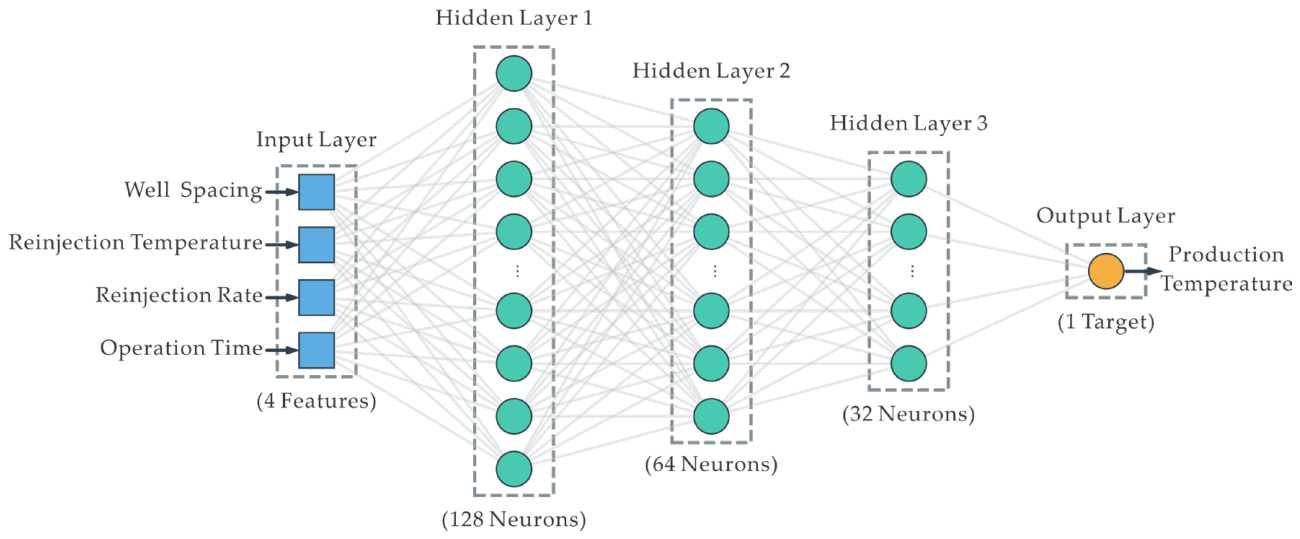
The hydrothermal flow in deep geothermal reservoirs during long-term injection-production cycles exhibits high nonlinearity and complexity, making it difficult for traditional shallow machine learning models to meet the accuracy requirements of high-dimensional optimization. Therefore, this study designed a deep feedforward neural network architecture (Figure 2):
  • Input layer: Contains 4 neurons, corresponding to the four preprocessed input features: well spacing, reinjection temperature, reinjection rate, and operation time.
  • Hidden layers: To fully extract the deep mapping relationship between the input data and the thermal breakthrough time, the model constructed a “funnel-shaped” deep network structure containing three hidden layers. The number of neurons in each hidden layer follows a step-wise decreasing design, which are 128, 64, and 32, respectively. A ReLU activation function is introduced after each hidden layer to enhance the nonlinear expression capability of the model and mitigate the vanishing gradient phenomenon. This decreasing topology acts as an information bottleneck, enforcing the network to extract a compressed, hierarchical representation of hydrothermal dynamics. This architecture inherently restricts over-parameterization and mitigates overfitting on the deterministic dataset [28].
  • Output layer: Contains 1 neuron, outputting the predicted value of the production temperature under specific scenarios and time nodes.

3.3. Model Training and Optimization Algorithm

To ensure physical consistency, this study introduces a physics-informed loss function (Ltotal) that embeds thermodynamic boundary conditions directly into the network training process. According to the thermodynamics of geothermal reinjection, the production temperature (Tprod) must not fall below the injection temperature (Tinj). The custom loss function is formulated as follows [19]:
L t o t a l = L m s e + λ L p h y
L p h y = 1 N i = 1 N ( max ( 0 , T i n j , i T p r o d , i ) ) 2
where Lmse measures the data fidelity of the thermal breakthrough trajectories; Lphy serves as the thermodynamic penalty term evaluating the degree of non-physical predictions; and λ is the penalty weight coefficient. The thermodynamic penalty is used as a soft constraint during network training. Its role is to reduce predictions that violate the basic thermal boundary within the bounded simulator-derived data domain, rather than to solve the governing hydrothermal equations directly as in standard PINNs. Therefore, the model should be regarded as a physics-constrained surrogate trained on numerical simulation data. In this study, λ was set to 1.0 to retain the thermodynamic soft constraint while maintaining the data-fitting capability of the DNN. To evaluate the influence of this empirical setting, a sensitivity test was conducted using λ = 0, 0.1, 1, and 10 under the same scenario-wise split. For consistency with the final selected surrogate model, the λ = 1 row in Table S1 was evaluated using the same trained DNN model reported in Table 2, whereas the other λ settings were independently retrained. The results are provided in Table S1. All tested settings achieved (R2 > 0.999), RMSE values below 0.05 °C, and a 0.00% non-physical prediction rate on the test set. The highest test-set accuracy occurred when λ = 0.1, whereas λ = 1 produced a slightly larger but still small prediction error. In addition, the global scans under different λ values identified favorable well spacings within a narrow range of approximately 456–462 m, with the same reinjection temperature of 20 °C and reinjection rate of 150 m3/h. This indicates that the main screening conclusion is not strongly controlled by the selected λ value. Therefore, λ = 1 was retained as a conservative setting for preserving the thermodynamic soft constraint in the physics-constrained surrogate workflow.
The model uses Mean Squared Error (MSE) for Lmse. Because the dataset is derived from partial differential equations and represents a smooth data space without random noise, Dropout and explicit regularization were omitted to maximize approximation of the physical hydrothermal response. The Adam optimizer updates weights using mini-batch gradient descent (batch size = 256) to balance computational efficiency and generalization. This configuration introduces moderate randomness, aiding in escaping local optima. The initial learning rate was 0.001 over 500 epochs. Predicted temperatures are restored to Celsius (°C) via denormalization.

4. Evaluation of the Deep Neural Network Prediction Model

4.1. Model Training and Convergence Analysis

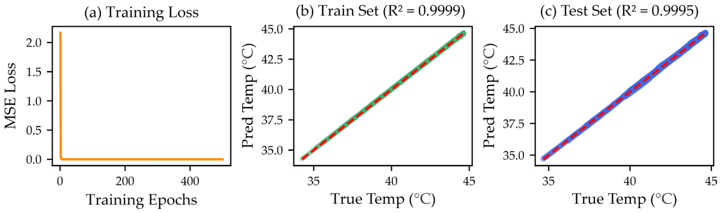
The convergence of the model is evaluated by monitoring the Mean Squared Error (MSE) loss function across training epochs. As shown in Figure 3a, using the Adam optimization algorithm, the training loss decreases rapidly during the initial stage and stabilizes after approximately 20 epochs. Within the 500 training epochs, the loss curve exhibits no oscillation or divergence, indicating that the network architecture and hyperparameter settings facilitate stable convergence during training.

4.2. Prediction Accuracy Assessment

To verify whether the model suffers from overfitting, this study extracted and compared the prediction results of the training set (80%) and the independent test set (20%). As shown in Figure 3b,c, in both the training and test sets, the production temperatures predicted by the DNN show high consistency with the numerical simulation values, with data points evenly distributed around the y = x diagonal. Statistical results indicate that the coefficients of determination (R2) of the model on the training and test sets are 0.9999 and 0.9995, respectively, with a Root Mean Square Error (RMSE) of 0.0351 °C on the test set. It should be noted that the high accuracy (R2 = 0.9995) achieved by this surrogate model on the test set is primarily attributed to the physical determinism of the underlying training data. Unlike field-measured data containing random measurement noise, the samples in this study originate from numerical simulations strictly governed by the partial differential equations of mass and energy conservation in porous media. Such deterministic data exhibit a smooth and continuous mapping manifold within the input parameter space. When a deep feedforward neural network possesses sufficient hidden layer dimensions, it can accurately reconstruct the noise-free nonlinear hydrothermal coupled evolution dynamics. Consequently, this validation accuracy objectively reflects the model’s approximation of the underlying physical mechanisms rather than extrapolative capability in heterogeneous field conditions.
To further evaluate the surrogate performance, additional benchmark regressors were trained and tested using the same input variables, scenario-wise split, and deterministic COMSOL-derived dataset. The benchmark models included support vector regression (SVR), random forest regression (RF), gradient boosting regression (GBRT), histogram-based gradient boosting regression (HGBR), and XGBoost. As shown in Table 2, SVR achieved the highest test-set accuracy, with (R2 = 0.9996), RMSE = 0.0310 °C, and MAE = 0.0195 °C. The physics-constrained DNN produced comparable accuracy, with (R2 = 0.9995), RMSE = 0.0351 °C, and MAE = 0.0227 °C, while requiring a substantially shorter prediction time than SVR. The tree-based ensemble models reproduced the general simulator response but showed larger errors than SVR and the DNN. No benchmark model produced non-physical test-set predictions below the reinjection temperature. These results indicate that the selected DNN provides an accurate and computationally efficient surrogate for continuous parameter-space screening, while the embedded thermodynamic penalty and post-processing boundary constraint preserve physical consistency during subsequent optimization.

4.3. Introduction of Physical Constraints

Purely data-driven black-box models occasionally generate extreme values that violate basic physical principles when performing high-dimensional spatial extrapolation predictions. According to the thermodynamic principles of geothermal reinjection systems, the outlet temperature of the production well cannot be lower than the temperature of the injected fluid at any evolutionary stage (TprodTinj). Therefore, this study introduces a hard physical boundary constraint at the model’s output end. During the execution of the three-dimensional full-parameter space scanning calculation, a post-processing truncation algorithm is employed to forcibly correct non-physical predicted values lower than the reinjection temperature, thereby further ensuring the engineering reliability of the global optimization results.
To evaluate the physical reliability of the surrogate model, the frequency of non-physical predictions (instances where the predicted production temperature is lower than the reinjection temperature, Tpred < Tinj) was quantified on the test set. The statistical result demonstrates an occurrence rate of 0.00% (0 instances). This result is governed by the network training mechanism and data characteristics. During the training phase, the physics-informed loss function imposes a thermodynamic penalty. Concurrently, the synthetic dataset derived from partial differential equations provides a noise-free, smooth thermodynamic manifold. This data structure enables the neural network to approximate the physical boundaries without data-induced oscillations [29]. Furthermore, to guarantee mathematical closure during the subsequent continuous parameter space optimization, a boundary constraint function (max(Tpred, Tinj)) is embedded into the predictive workflow.

5. Evolution Laws of Injection-Production Parameters and Optimization of Exploitation Schemes

5.1. Local Sensitivity Analysis of Exploitation Parameters

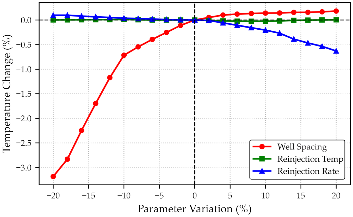
Taking the 50th year of system operation as the baseline, the control variable method is employed to analyze the perturbation degree of each parameter variation on the production temperature (Figure 4). The results indicate that the sensitivity of the parameters to production temperature is ranked as follows: well spacing > injection rate > injection temperature. The reinjection flow rate exhibits a negative correlation with the production temperature, whereas the reinjection temperature shows a positive correlation. The impact of well spacing on production temperature demonstrates nonlinear characteristics. Decreasing well spacing below 500 m induces a temperature decline; conversely, increasing well spacing beyond 10% of the baseline results in a temperature plateau. Physically, as the cold water front diffuses radially in the porous medium, the swept rock volume is proportional to the square of the propagation radius. Consequently, monotonically increasing the injection-production well spacing yields a diminishing marginal benefit in delaying the thermal breakthrough time [30,31,32]. It is noted that this parameter sensitivity ranking reflects the gradient response of the system around a specific operational baseline, rather than a global variance-based metric across the entire multi-dimensional domain.

5.2. Multi-Parameter Response Characteristics of Thermal Breakthrough Time

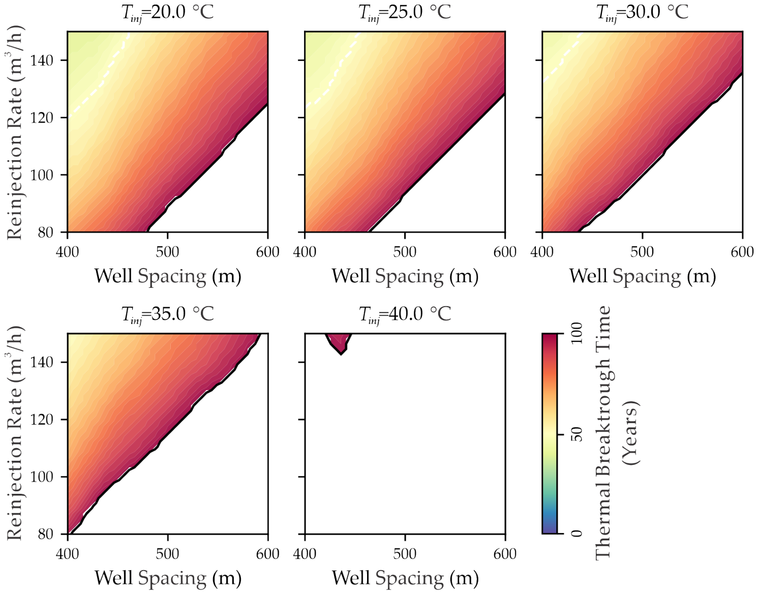
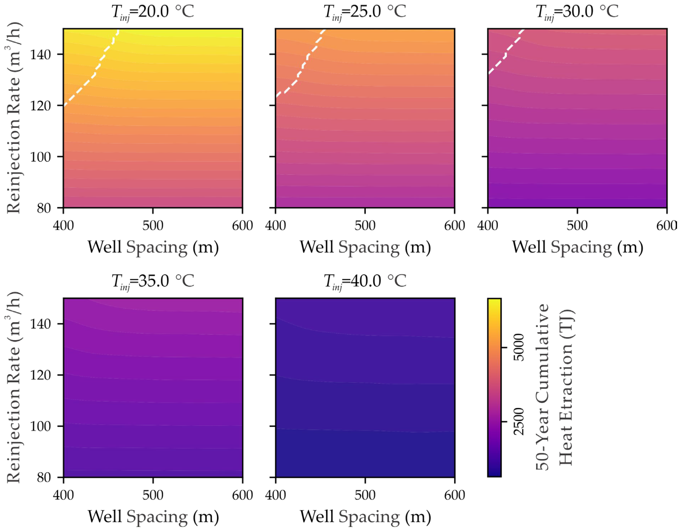
Thermal breakthrough is defined as a 2.0 °C decrease in the production well temperature. Figure 5 illustrates the thermal breakthrough time evolution in the two-dimensional space of well spacing and reinjection rate, with reinjection temperatures ranging from 20 °C to 40 °C. Reducing the reinjection temperature compresses the operational boundary of the geothermal reservoir. In Figure 5, the dashed line delineates the critical thermal breakthrough boundary within the 50-year design life. As the reinjection temperature decreases from 40 °C to 20 °C, this boundary expands. At 40 °C, none of the development schemes experience thermal breakthrough within 50 years; when the temperature drops to 20 °C, the earliest observed thermal breakthrough occurs at 20 years. From a thermodynamic perspective, reducing the injection temperature increases the injection-production thermal gradient. To achieve local thermal equilibrium, the injected cold fluid must absorb enthalpy from a larger volume of the surrounding rock matrix [33]. Although the macroscopic hydraulic transport velocity remains relatively stable under a constant injection rate, the increased enthalpy demand inherently accelerates the propagation of the thermal front, thereby advancing the thermal breakthrough time [34,35]. Therefore, low-temperature reinjection requires a corresponding expansion of the well pattern spacing to match the increased heat transfer demands [36,37].
The 2.0 °C temperature-decline threshold is used in this study as an engineering warning criterion for identifying the onset of thermal breakthrough within the 50-year design life, rather than as an absolute physical failure boundary. To evaluate the influence of this criterion, an additional threshold-sensitivity test was conducted using 1.0, 2.0, and 3.0 °C temperature-decline thresholds. The results are provided in Table S2. The selected threshold affects both the absolute breakthrough time and the favorable spacing identified by the comprehensive evaluation factor. In the DNN-based continuous scan, the favorable well spacing shifts from approximately 492 m under the stricter 1.0 °C threshold to approximately 462 m under the adopted 2.0 °C threshold and approximately 441 m under the more relaxed 3.0 °C threshold. This indicates that the reported favorable spacing is threshold-dependent and should be interpreted within the adopted engineering criterion. However, the local COMSOL validation results show physically consistent behavior across all thresholds: increasing the temperature-decline threshold delays the identified breakthrough time, and increasing well spacing delays thermal breakthrough. Under the adopted 2.0 °C criterion, the 460–462 m cases did not reach the 2.0 °C decline threshold within the 50-year design life, whereas the 430 and 440 m cases experience thermal breakthrough before 50 years and the 450 m case is close to the design boundary. Therefore, the 2.0 °C criterion is retained as a moderate engineering warning threshold, and the recommended spacing interval is interpreted as conditional on this design criterion.

5.3. Evaluation of Cumulative Heat Production

To evaluate the practical exploitation benefits of each scheme, this study quantifies the cumulative heat production of the system over its design life using thermodynamic principles. The calculation formula is as follows [38]:
H = i = 1 n q × ρ × c p × ( T a v g . i T i n j ) × Δ t × 8760 × 10 12
where q is the reinjection flow rate (m3/h); ρ is the fluid density (kg/m3); cp is the specific heat capacity of the fluid (J/(kg⋅K)); Tinj is the injection temperature (°C); Tavg.i = (Ti + Ti−1)/2; and Δt is the operation time step (yr). Because q is expressed in (m3/h), whereas Δt is expressed in years, the calculation explicitly uses (8760 h/yr) to convert the annual time step into hours. The resulting heat quantity is converted from J to TJ using a factor of (10−12). The application of this formulation is predicated on the assumption of macroscopic mass conservation, wherein the fluid production rate strictly equals the reinjection rate throughout the operational horizon.
The 50-year cumulative heat production under various exploitation conditions is calculated using Equation (6) (Figure 6). The results indicate that regardless of the reinjection temperature and flow rate, the maximum cumulative heat production consistently occurs under the condition of the maximum well spacing (600 m). Physically, expanding the well spacing increases the total reservoir volume swept by the circulating fluid. This maximizes the extraction of stored sensible heat from the rock matrix prior to the onset of thermal interference between the injection and production wells [39]. However, in field geothermal engineering deployment, continuously expanding the injection-production well spacing leads to an increase in directional drilling and completion costs [40]. Simultaneously, the increased formation hydraulic pressure drop caused by long-distance seepage elevates the long-term energy consumption of the injection pump required to maintain the system’s circulation flow rate [41]. Therefore, relying solely on cumulative heat production as a single evaluation metric makes it difficult to achieve the optimal configuration of physical performance and economic benefits in engineering planning.

5.4. Optimization of Exploitation Schemes

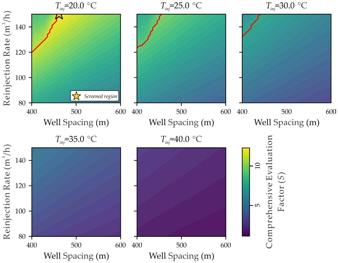
To address the physical trade-off among high heat production, high well construction costs, and short lifespan, this study constructs a comprehensive evaluation factor, S. While pursuing maximum heat production (H), this metric introduces well spacing (D) in the denominator to constrain well construction costs and incorporates a nonlinear reservoir lifespan penalty term, (t/L)n, for schemes experiencing early thermal short-circuiting. The formula is as follows:
S = H D × ( t L ) n
where H is the cumulative heat production indicator, D is the well spacing, t is the thermal breakthrough time, L is the design life, and n is the penalty factor (n = 2). For operational scenarios where the production-temperature decline does not reach the critical breakthrough threshold within the 50-year design life, the parameter t is assigned a value equal to L (t = 50), rendering the lifespan penalty term to 1.0.
Based on the principle of the quadratic penalty function, this study sets the nonlinear lifespan penalty exponent to n = 2 [42]. Mathematically, a quadratic penalty ensures C1 continuity of the objective function across the parameter space, preventing non-differentiable singularities during the continuous spatial optimization process [42]. From an engineering perspective, the economic viability of a geothermal doublet system degrades non-linearly with premature thermal breakthrough. A quadratic exponent applies a statistically heavier weight against operational scenarios that induce early thermal short-circuiting, a process consistent with the accelerated financial depreciation associated with premature well abandonment [36,43]. Compared to higher-order penalties (n ≥ 3), this configuration prevents the over-penalization of schemes experiencing late-stage thermal breakthrough, preserving the gradient smoothness of the evaluation factor during global optimization [19,44].
Based on the DNN prediction model retrained using the corrected 100 mD equivalent aquifer permeability, a global scan was conducted over the three-dimensional parameter space, including well spacing of 400–600 m, reinjection temperature of 20–40 °C, and reinjection rate of 80–150 m3/h. The surrogate-based scan identified a favorable region near a well spacing of 462 m, a reinjection temperature of 20 °C, and a reinjection flow rate of 150 m3/h (Figure 7). This result should be interpreted as a rapid surrogate-screening outcome rather than as a precise simulator-validated optimum. Because the original COMSOL design contained only three well-spacing levels, namely 400, 500, and 600 m, additional local simulator checks were required to evaluate whether the predicted favorable spacing was affected by sparse spacing coverage.
In the equivalent porous medium model, the movement of the thermal front is controlled by Darcy flow and heat exchange with the rock matrix [30,34]. Therefore, the production-temperature response is expected to vary continuously with well spacing within the bounded simulator domain. However, physical continuity alone does not eliminate interpolation uncertainty caused by sparse sampling. For this reason, the surrogate-screened spacing region around 462 m was further evaluated using additional COMSOL simulations, as described in the following subsection.

5.5. Local COMSOL Validation of the Surrogate-Screened Well-Spacing Region

To evaluate whether the surrogate-screened spacing region was affected by the sparse original well-spacing grid, nine additional COMSOL simulations were performed around the predicted favorable region. The validation cases used D = 430, 440, 450, 460, 462, 470, 480, 490, and 500 m, while the reinjection temperature and reinjection rate were fixed at 20 °C and 150 m3/h, respectively. These cases were generated after the surrogate-based screening and were not used for DNN training. They therefore provide an independent numerical check of the local response surface around the surrogate-identified spacing region.
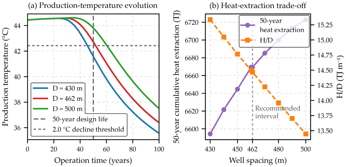
The validation results show a continuous thermal response with increasing well spacing (Table 3). At 50 years, the production-temperature decline decreases from 2.842 °C at 430 m to 0.617 °C at 500 m, and the 2.0 °C thermal breakthrough time is delayed from 46 to 61 years. The 430 and 440 m cases experience 2.0 °C breakthrough before the 50-year design life, whereas the 450 m case is close to the design boundary. In contrast, the 460 and 462 m cases remain below the 2.0 °C decline threshold during the 50-year design life, with 50-year temperature declines of 1.722 and 1.713 °C, respectively.
The 50-year cumulative heat extraction increases slightly from 6594.2 TJ at 430 m to 6722.9 TJ at 500 m as well spacing increases. However, because the increase in cumulative heat extraction is small compared with the increase in well spacing, the H/D term decreases from 15.335 to 13.446 TJ/m. Therefore, the local COMSOL validation supports the physical continuity of the response surface, but it does not support treating 462 m as a unique deterministic optimum. Under the present equivalent-porous-medium simulator and the adopted evaluation factor, the engineering recommendation is therefore expressed as an approximately 460–462 m well-spacing interval rather than as a single precise spacing value.
Figure 8 compares three representative cases, namely 430, 462, and 500 m. The 430 m case reaches the 2.0 °C decline threshold before the 50-year design life, whereas the 462 and 500 m cases remain below the threshold within 50 years. After the design life, temperature decline accelerates as the thermal front becomes more strongly connected to the production well. This result indicates that the surrogate model is useful for narrowing the design space, whereas targeted COMSOL simulations are required before reporting a final engineering spacing recommendation.

5.6. Limitations and Engineering Applicability

Although the proposed DNN surrogate provides an efficient tool for screening injection-production parameters, several limitations should be noted. First, the DNN was trained on COMSOL-derived synthetic outputs rather than on independent field production records. Therefore, the reported accuracy reflects the model’s ability to approximate a deterministic simulator response within the predefined operating domain, rather than its direct predictive robustness under uncalibrated field conditions. Field-scale application would require calibration using production-temperature records, pressure monitoring, reinjection tests, tracer tests, and history matching.
Second, the effective diversity of the training database is controlled by the 120 independent COMSOL scenarios, rather than by the total number of annual time-series records. The 12,000 samples represent structured temporal outputs derived from these scenarios. A larger simulation database, preferably generated through adaptive sampling or active-learning strategies, would improve the robustness of the surrogate response surface and reduce interpolation uncertainty in higher-dimensional design spaces.
Third, the Ordovician fracture-karst reservoir was represented using an equivalent porous medium. The adopted aquifer permeability of 100 mD and porosity of 0.04 should therefore be interpreted as upscaled effective macroscopic parameters rather than as primary matrix properties. Actual karst reservoirs may contain discrete fractures, karst conduits, and anisotropic hydraulic pathways that accelerate cold-water migration and cause earlier thermal short-circuiting than predicted by a homogeneous EPM model. Future work should incorporate dual-porosity or discrete-fracture representations to quantify the influence of preferential flow paths on thermal-front propagation.
Finally, the current sensitivity analysis remains primarily local and engineering-oriented. Although threshold and penalty-weight sensitivity tests were added in this revision, global variance-based techniques such as Sobol analysis or Morris screening were not implemented because they require a larger and more densely sampled simulation ensemble. These methods should be considered in future studies once a broader simulation database and parameter-uncertainty framework are available.

5.7. Engineering Implications for the Qihe Geothermal Field

The combined DNN screening and local COMSOL validation provide pre-feasibility design guidance for the Ordovician carbonate karst geothermal reservoir in the Qihe field. Under the present equivalent-porous-medium assumption and the adopted 2.0 °C thermal breakthrough criterion, the surrogate-based global scan identified a favorable operating region near 462 m well spacing, 20 °C reinjection temperature, and 150 m3/h reinjection rate. The additional COMSOL validation cases further show that the approximately 460–462 m spacing interval avoids the 2.0 °C decline threshold within the 50-year design life while retaining relatively high heat-extraction efficiency per unit well spacing.
This interval should be used as a preliminary spatial deployment reference for new doublet systems, not as a final construction spacing or a field-validated optimum. In practical engineering design, the recommended interval needs to be adjusted according to site-specific fracture development, hydraulic connectivity, well completion conditions, reinjection pressure limits, pumping energy consumption, and surface heat-demand constraints. The reinjection temperature of 20 °C and reinjection rate of 150 m3/h should likewise be interpreted as screening-level operating conditions within the tested design domain rather than universal operating prescriptions.
The practical value of the proposed workflow lies in rapidly narrowing the parameter space before expensive simulator refinement and field-scale calibration. Once additional production monitoring, pressure data, reinjection-test results, and tracer-test constraints become available, the COMSOL model and the DNN surrogate should be recalibrated. The workflow can then be updated iteratively to support site-specific well-pattern design and long-term reinjection management.

6. Conclusions

This study proposes an optimization framework for geothermal reinjection systems that integrates hydrothermal coupled simulation with deep neural networks (DNN). Using the Qihe geothermal field as a case study, the main findings are as follows:
  • A DNN surrogate was trained using COMSOL-derived hydrothermal simulation outputs and evaluated with a scenario-wise split. The model achieved R2 = 0.9995 and RMSE = 0.0351 °C on the test set, indicating accurate approximation of the deterministic simulator response within the predefined parameter domain. This result should be interpreted as bounded-domain surrogate accuracy rather than field-scale predictive robustness.
  • The local sensitivity response of exploitation parameters to system thermal attenuation was ranked as follows: well spacing > reinjection flow rate > reinjection temperature. Governed by the radial diffusion mechanism of the cold water front in porous media, increasing the injection-production well spacing exhibits a nonlinear diminishing marginal benefit in delaying thermal breakthrough. Concurrently, lowering the reinjection temperature increases the enthalpy demand of the rock matrix, which accelerates the propagation of the thermal front and advances the thermal breakthrough time.
  • A comprehensive evaluation system integrating cumulative heat production, well construction costs, and a nonlinear lifespan penalty was established. The surrogate-based global scan identified a favorable spacing region near 462 m under the corrected 100 mD equivalent aquifer permeability. Additional COMSOL simulations around this region confirmed that the 460–462 m cases avoided 2.0 °C thermal breakthrough within the 50-year design life while retaining relatively high heat-extraction efficiency per unit well spacing. Therefore, the final engineering recommendation is expressed as an approximately 460–462 m spacing interval rather than as a single deterministic optimum.

Supplementary Materials

The following supporting information can be downloaded at: https://www.mdpi.com/article/10.3390/app16136291/s1, Table S1: Sensitivity of DNN performance and surrogate-screened spacing to the thermodynamic penalty weight λ; Table S2: Sensitivity of thermal-breakthrough interpretation to the temperature-decline threshold.

Author Contributions

Conceptualization, L.D. and K.L.; methodology, L.D.; software, K.L.; validation, L.D., K.L., C.Z. and F.Z.; formal analysis, L.D.; investigation, F.L., L.C. and F.Z.; resources, L.D.; data curation, F.L. and Y.J.; writing—original draft preparation, L.D.; writing—review and editing, K.L. and C.Z.; visualization, K.L., F.L., L.C., Y.J. and Z.Z.; supervision, L.D.; project administration, F.L. and Y.J.; funding acquisition, L.D. All authors have read and agreed to the published version of the manuscript.

Funding

This research is supported by the National Key Research and Development Program of China (2021YFA0716003).

Data Availability Statement

The raw data involved in this study include sensitive information and confidential content provided by collaborating institutions. According to contractual agreements with these partners, the data cannot be fully disclosed at this time. Researchers requiring access for academic purposes may submit a request via email to the corresponding author (likefu553@163.com). After a review, we will provide the data in compliance with legal and institutional guidelines.

Acknowledgments

The authors thank the anonymous reviewers for their constructive comments and suggestions.

Conflicts of Interest

Authors L.D., F.L, and Y.J. were employed by the company SINOPEC Star Petroleum Corporation Limited. The authors declare that the research was conducted in the absence of any commercial or financial relationships that could be construed as potential conflicts of interest.

References

  1. Huang, Y.; Pang, Z.; Kong, Y.; Watanabe, N. Assessment of the High-Temperature Aquifer Thermal Energy Storage (HT-ATES) Potential in Naturally Fractured Geothermal Reservoirs with a Stochastic Discrete Fracture Network Model. J. Hydrol. 2021, 603, 127188. [Google Scholar]
  2. Sun, H.; Mao, X.; Wu, C.; Guo, D.; Wang, H.; Sun, S.; Zhang, Y.; Luo, L. Geothermal Resources Exploration and Development Technology: Current Status and Development Direction. Earth Sci. Front. 2024, 31, 400–411. (In Chinese) [Google Scholar]
  3. Fan, B.; Ye, H.; Bai, X.; Zhou, G.; Zhuang, Y. Indicative Significance of Geothermal Fluid Dynamics on the Balance of Geothermal Water Injection and Extraction in Wentang Geothermal Field. Geol. Rev. 2024, 70, 195–198. (In Chinese) [Google Scholar]
  4. Yang, F.; Song, H.; Zhao, Q.; Tan, J. Dynamic Monitoring of Artificial Recharge of Groundwater and Evaluation of Geothermal Resources. Geotech. Eng. Tech. 2025, 39, 383–390. (In Chinese) [Google Scholar]
  5. Huang, Y.; Cheng, Y.; Ren, L.; Tian, F.; Pan, S.; Wang, K.; Wang, J.; Dong, Y.; Kong, Y. Assessing the Geothermal Resource Potential of an Active Oil Field by Integrating a 3D Geological Model with the Hydro-Thermal Coupled Simulation. Front. Earth Sci. 2022, 9, 787057. [Google Scholar] [CrossRef]
  6. Ding, R.; Zhu, C.; Cao, Q.; Fang, C.; Yang, Y.; Jiang, X. Numerical Simulation of Buried Hill Geothermal Resources Exploitation in Hejian Area. Acta Geosci. Sin. 2023, 44, 248–256. (In Chinese) [Google Scholar]
  7. Liu, F.; Kang, F.; Liu, X.; Shi, Q.; Zheng, T.; Qin, P.; Gao, Z. Constraint of Thermal Breakthrough on Rational Well Spacing of Karst Thermal Reservoir: A Case Study of Heze Geothermal Field. Acta Geol. Sin. 2024, 98, 3149–3168. (In Chinese) [Google Scholar]
  8. Zhang, S.; Zhao, Y.; Lu, B.; Zong, Z.; Gai, Y.; Wang, B.; Gao, X. Development of Downhole Stratified Multi-Parameter Monitoring System and Its Application in Geothermal Reinjection Wells. Miner. Explor. 2025, 16, 606–613. (In Chinese) [Google Scholar]
  9. Wang, T.; Hu, J.; Liu, C.; Gao, Z.; Tang, X. The Effect of Plane Heterogeneity on the Reinjection Flow of Geothermal Reservoir: A Case Study of the Guantao Formation in Baoding City. Geol. Explor. 2025, 61, 431–440. (In Chinese) [Google Scholar]
  10. Esen, H.; Inalli, M.; Sengur, A.; Esen, M. Performance Prediction of a Ground-Coupled Heat Pump System Using Artificial Neural Networks. Expert Syst. Appl. 2008, 35, 1940–1948. [Google Scholar] [CrossRef]
  11. Esen, H.; Inalli, M. Modelling of a Vertical Ground Coupled Heat Pump System by Using Artificial Neural Networks. Expert. Syst. Appl. 2009, 36, 10229–10238. [Google Scholar] [CrossRef]
  12. Zhang, Y.; Zhou, L.; Hu, Z.; Yu, Z.; Hao, S.; Lei, Z.; Xie, Y. Prediction of Layered Thermal Conductivity Using Artificial Neural Network in Order to Have Better Design of Ground Source Heat Pump System. Energies 2018, 11, 1896. [Google Scholar] [CrossRef]
  13. Shahdi, A.; Lee, S.; Karpatne, A.; Nojabaei, B. Exploratory Analysis of Machine Learning Methods in Predicting Subsurface Temperature and Geothermal Gradient of Northeastern United States. Geotherm. Energy 2021, 9, 18. [Google Scholar] [CrossRef]
  14. Suzuki, A.; Fukui, K.; Onodera, S.; Ishizaki, J.; Hashida, T. Data-Driven Geothermal Reservoir Modeling: Estimating Permeability Distributions by Machine Learning. Geosciences 2022, 12, 130. [Google Scholar] [CrossRef]
  15. Ahmadi, M. Interpretable Machine Learning for High-Accuracy Reservoir Temperature Prediction in Geothermal Energy Systems. Energies 2025, 18, 3366. [Google Scholar] [CrossRef]
  16. Khedekar, V.V.; Memon, A.R.A.N.; Pal, M. Efficient Geothermal Reservoir Simulation Using Deep Learning Surrogates and Multiscale Interpolation Techniques. Processes 2026, 14, 1248. [Google Scholar] [CrossRef]
  17. Du, L.; Du, J.; Fang, Z.; Shah, S.Y.A.; Kablan, O.A.B.K.; Zhang, B.; Tan, J. A Recurrent Neural Network Surrogate Model with Few-Shot Strategy for CO2 Storage in Deep Subsurface Saline Aquifer with Limited Direct Numerical Simulation Samples. Lithosphere 2026, 2026, lithosphere_2025_139. [Google Scholar] [CrossRef]
  18. Willard, J.; Jia, X.; Xu, S.; Steinbach, M.; Kumar, V. Integrating Physics-Based Modeling with Machine Learning: A Survey. arXiv 2020, arXiv:2003.04919. [Google Scholar]
  19. Karniadakis, G.E.; Kevrekidis, I.G.; Lu, L.; Perdikaris, P.; Wang, S.; Yang, L. Physics-Informed Machine Learning. Nat. Rev. Phys. 2021, 3, 422–440. [Google Scholar] [CrossRef]
  20. Parsa, S.M. Physics-Informed Machine Learning Meets Renewable Energy Systems: A Review of Advances, Challenges, Guidelines, and Future Outlooks. Appl. Energy 2025, 402, 126925. [Google Scholar] [CrossRef]
  21. Qin, Z.; Jiang, A.; Faulder, D.; Cladouhos, T.T.; Jafarpour, B. Physics-Guided Deep Learning for Prediction of Energy Production from Geothermal Reservoirs. Geothermics 2024, 116, 102824. [Google Scholar]
  22. Bear, J. Dynamics of Fluids in Porous Media; Courier Corporation: Washington, DC, USA, 1988. [Google Scholar]
  23. Nield, D.A.; Bejan, A. Convection in Porous Media; Springer International Publishing: Cham, Switzerland, 2017. [Google Scholar]
  24. Jia, Y.; Su, Y.; Sui, S.; Jia, W.; Li, Z.; Yang, Z.; Wang, X.; Gao, F.; Ji, H.; Bao, Z. Lithofacies Palaeogeographic Characteristics and Evolution of the Ordovician in Western Shandong-Eastern Henan Area. J. Palaeogeogr. Chin. Ed. 2023, 25, 133–147. [Google Scholar]
  25. Sui, S.; Yang, Z.; Zhao, Y.; Jia, Y.; Su, Y.; Wang, X.; Gao, F.; Ji, H.; Bao, Z. Evolution and Main Controlling Factors of the Ordovician Karst Thermal Reservoir in Western Shandong-Eastern Henan Area. J. Palaeogeogr. Chin. Ed. 2023, 25, 1364–1378. [Google Scholar]
  26. Zhang, B.; Wang, S.; Kang, F.; Wu, Y.; Li, Y.; Gao, J.; Yuan, W.; Xing, Y. Heat Accumulation Mechanism of the Gaoyang Carbonatite Geothermal Field, Hebei Province, North China. Front. Earth Sci. 2022, 10, 858814. [Google Scholar] [CrossRef]
  27. Fan, J.; Chen, W.; Tan, X.; Sui, J.; Liu, Q.; Chen, H.; Zhang, F.; Chen, G.; Xu, Z. Water Storage Capacity of Ordovician Limestone Aquifer and Hydrogeological Response Mechanism of Deep Reinjection in North China. Water 2025, 17, 1982. [Google Scholar] [CrossRef]
  28. Tishby, N.; Zaslavsky, N. Deep Learning and the Information Bottleneck Principle. In Proceedings of the 2015 IEEE Information Theory Workshop (ITW); IEEE: New York, NY, USA, 2015; pp. 1–5. [Google Scholar]
  29. Raissi, M.; Perdikaris, P.; Karniadakis, G.E. Physics-Informed Neural Networks: A Deep Learning Framework for Solving Forward and Inverse Problems Involving Nonlinear Partial Differential Equations. J. Comput. Phys. 2019, 378, 686–707. [Google Scholar] [CrossRef]
  30. Gringarten, A.C. Reservoir Lifetime and Heat Recovery Factor in Geothermal Aquifers Used for Urban Heating. Pure Appl. Geophys. 1978, 117, 297–308. [Google Scholar] [CrossRef]
  31. Banks, D. Thermogeological Assessment of Open-Loop Well-Doublet Schemes: A Review and Synthesis of Analytical Approaches. Hydrogeol. J. 2009, 17, 1149–1155. [Google Scholar]
  32. Babaei, M.; Nick, H.M. Performance of Low-Enthalpy Geothermal Systems: Interplay of Spatially Correlated Heterogeneity and Well-Doublet Spacings. Appl. Energy 2019, 253, 113569. [Google Scholar]
  33. Bödvarsson, G.S.; Tsang, C.F. Injection and Thermal Breakthrough in Fractured Geothermal Reservoirs. J. Geophys. Res. Solid Earth 1982, 87, 1031–1048. [Google Scholar] [CrossRef]
  34. Woods, A.W. Flow in Porous Rocks: Energy and Environmental Applications; Cambridge University Press: Cambridge, UK, 2014. [Google Scholar]
  35. Aliyu, M.D.; Chen, H.-P. Sensitivity Analysis of Deep Geothermal Reservoir: Effect of Reservoir Parameters on Production Temperature. Energy 2017, 129, 101–113. [Google Scholar] [CrossRef]
  36. Kong, Y.; Pang, Z.; Shao, H.; Kolditz, O. Optimization of Well-Doublet Placement in Geothermal Reservoirs Using Numerical Simulation and Economic Analysis. Environ. Earth Sci. 2017, 76, 118. [Google Scholar] [CrossRef]
  37. Kamila, Z.; Kaya, E.; Zarrouk, S.J. Reinjection in Geothermal Fields: An Updated Worldwide Review 2020. Geothermics 2021, 89, 101970. [Google Scholar] [CrossRef]
  38. Muffler, P.; Cataldi, R. Methods for Regional Assessment of Geothermal Resources. Geothermics 1978, 7, 53–89. [Google Scholar] [CrossRef]
  39. Asai, P.; Panja, P.; Velasco, R.; McLennan, J.; Moore, J. Fluid Flow Distribution in Fractures for a Doublet System in Enhanced Geothermal Systems (EGS). Geothermics 2018, 75, 171–179. [Google Scholar] [CrossRef]
  40. Daniilidis, A.; Nick, H.M.; Bruhn, D.F. Interdependencies between Physical, Design and Operational Parameters for Direct Use Geothermal Heat in Faulted Hydrothermal Reservoirs. Geothermics 2020, 86, 101806. [Google Scholar] [CrossRef]
  41. Zinsalo, J.M.; Lamarche, L.; Raymond, J. Design and Optimization of Multiple Wells Layout for Electricity Generation in a Multi-Fracture Enhanced Geothermal System. Sustain. Energy Technol. Assess. 2021, 47, 101365. [Google Scholar] [CrossRef]
  42. Nocedal, J.; Wright, S. Numerical Optimization; Springer Series in Operations Research; Springer: Berlin/Heidelberg, Germany, 2006. [Google Scholar]
  43. Beckers, K.F.; Lukawski, M.Z.; Anderson, B.J.; Moore, M.C.; Tester, J.W. Levelized Costs of Electricity and Direct-Use Heat from Enhanced Geothermal Systems. J. Renew. Sustain. Energy 2014, 6, 013141. [Google Scholar] [CrossRef]
  44. Bangerth, W.; Klie, H.; Wheeler, M.F.; Stoffa, P.L.; Sen, M.K. On Optimization Algorithms for the Reservoir Oil Well Placement Problem. Comput. Geosci. 2006, 10, 303–319. [Google Scholar] [CrossRef]
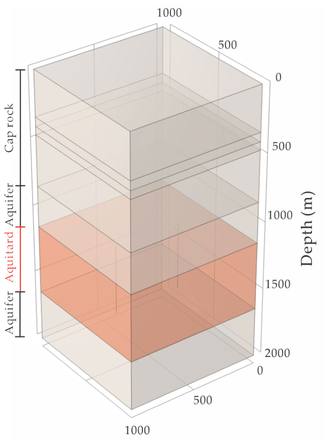
Figure 1. Stratigraphic model of Qihe. Different colors indicate the caprock, aquitards, and target aquifer in the conceptual stratigraphic model.
Applsci 16 06291 g001
Figure 2. Network architecture of the deep neural network (DNN) model.
Applsci 16 06291 g002
Figure 3. Training convergence and predictive performance of the deep neural network (DNN) model. (a) Training loss; (b) observed versus predicted production temperature for the training set; (c) observed versus predicted production temperature for the test set.
Applsci 16 06291 g003
Figure 4. Local one-factor sensitivity of production temperature to injection-production parameters at the 50th year.
Applsci 16 06291 g004
Figure 5. Thermal breakthrough time under different reinjection temperatures. The thermal breakthrough criterion is defined as a 2.0 °C decline in production temperature. The white dashed line denotes the 50-year thermal-breakthrough boundary.
Applsci 16 06291 g005
Figure 6. Cumulative heat production over 50 years of exploitation under different reinjection temperatures. The white dashed line denotes the 50-year thermal-breakthrough boundary.
Applsci 16 06291 g006
Figure 7. Comprehensive evaluation factor under different reinjection temperatures. The red line denotes the 50-year thermal-breakthrough boundary, and the star denotes the surrogate-screened favorable region near 462 m before local COMSOL validation.
Applsci 16 06291 g007
Figure 8. Temperature evolution and cumulative heat extraction for representative locally validated well-spacing cases of 430, 462, and 500 m under Tinj = 20 °C and q = 150 m3/h. (a) Production-temperature evolution; (b) 50-year cumulative heat extraction and heat extraction per unit well spacing.
Applsci 16 06291 g008
Table 1. Petrophysical properties of the caprock and geothermal reservoir.
LayerDensity
(Kg·m−3)
Thermal Conductivity
(W·(m·K)−1)
Specific Heat Capacity
(J·(kg·K)−1)
Permeability
(mD)
Porosity
Cap rock23002.19000.010.1
Aquitard27003.5850100.01
Aquifer27003.58501000.04
Table 2. Benchmark comparison between the DNN surrogate and alternative machine-learning regressors under the same scenario-wise split.
ModelR2RMSE (°C)MAE (°C)Non-Physical Prediction Rate (%)Prediction Time (s)
SVR0.99960.03100.01950.000.5317
DNN physics-constrained0.99950.03510.02270.000.0027
HGBR0.98800.18000.09280.000.0167
XGBoost0.97980.23360.16410.000.0038
RF0.97330.26890.14120.000.0915
GBRT0.96600.30360.20100.000.0057
Table 3. Local COMSOL validation of well-spacing effects near the surrogate-screened favorable region (Tinj = 20 °C, q = 150 m3/h).
Well Spacing
(m)
T0
(°C)
T50
(°C)
T100
(°C)
50-Year Decline
(°C)
2 °C Breakthrough Time
(yr)
50-Year Heat Extraction
(TJ)
H/D
(TJ/m)
43044.42541.58335.5622.842466594.215.335
44044.42541.95435.8122.471486621.615.049
45044.42542.31136.0862.114506644.714.766
46044.42542.70336.3581.722526669.414.499
46244.42542.71236.3911.713526669.314.435
47044.42543.00236.6261.423546685.214.224
48044.42543.28636.9251.139566700.013.958
49044.42543.57937.2100.846596713.513.701
50044.42543.80837.5080.617616722.913.446
Disclaimer/Publisher’s Note: The statements, opinions and data contained in all publications are solely those of the individual author(s) and contributor(s) and not of MDPI and/or the editor(s). MDPI and/or the editor(s) disclaim responsibility for any injury to people or property resulting from any ideas, methods, instructions or products referred to in the content.