Rotation-Equivariant Feature Learning on Polar BEV for Robust LiDAR Place Recognition

Abstract

LiDAR-based place recognition is critical for long-term autonomous navigation in Global Navigation Satellite System (GNSS)-denied environments, yet existing methods struggle to balance accuracy and efficiency under substantial yaw rotations. This paper proposes a robust framework based on a multi-channel polar bird’s-eye-view (BEV) representation. Under yaw-dominated revisits, the polar BEV image transforms yaw rotation into cyclic column shifts, providing a useful structural prior for rotation-equivariant feature extraction. Raw point clouds are projected onto polar BEV grids encoding density, height, and intensity. A rotation-equivariant feature extractor comprising a Radial Compression Module and a rotation-equivariant Transformer module captures long-range azimuthal dependencies via Conditional Positional Encoding and Circular Relative-Position Bias. The equivariant features are aggregated by NetVLAD into a compact global descriptor, trained end-to-end with a hard-example mining triplet loss. Extensive experiments on the public KITTI and NCLT datasets, as well as our self-constructed LiDAR Place Recognition Revisit (LPRR) dataset, demonstrate competitive performance on KITTI and superior performance on NCLT and LPRR among the compared methods. The proposed framework achieves a favorable trade-off between performance and computational cost, and shows promising cross-dataset generalization on the evaluated NCLT and LPRR datasets without fine-tuning.

1. Introduction

Place recognition refers to the capability of determining whether the currently observed environmental information corresponds to a location previously visited by the system. As a key technology in the autonomous navigation module of self-driving vehicles, place recognition provides reliable loop-closure cues for unmanned ground vehicles (UGVs), thereby effectively suppressing localization drift and enabling long-term stable operation in Global Navigation Satellite System (GNSS)-denied environments (e.g., forests, mountainous areas, underground tunnels) [1]. It thus constitutes the foundation for achieving global localization. However, among the various challenges in real-world deployment, robustness to large yaw rotations—such as those encountered at intersections and during reverse traversals—remains particularly critical yet under-addressed, as it directly determines whether a loop closure can be established under substantial viewpoint changes.

Depending on the type of environmental perception sensor employed, place recognition is primarily divided into two categories: Visual Place Recognition (VPR) and LiDAR Place Recognition (LPR). The former relies on images acquired by cameras and is susceptible to factors such as illumination variations, weather conditions, and lack of texture. The latter, in contrast, is based on 3D point cloud data and offers inherent advantages including robustness to lighting changes, well-defined geometric structures, and reliable depth information, making it particularly suitable for place recognition in outdoor scenarios.

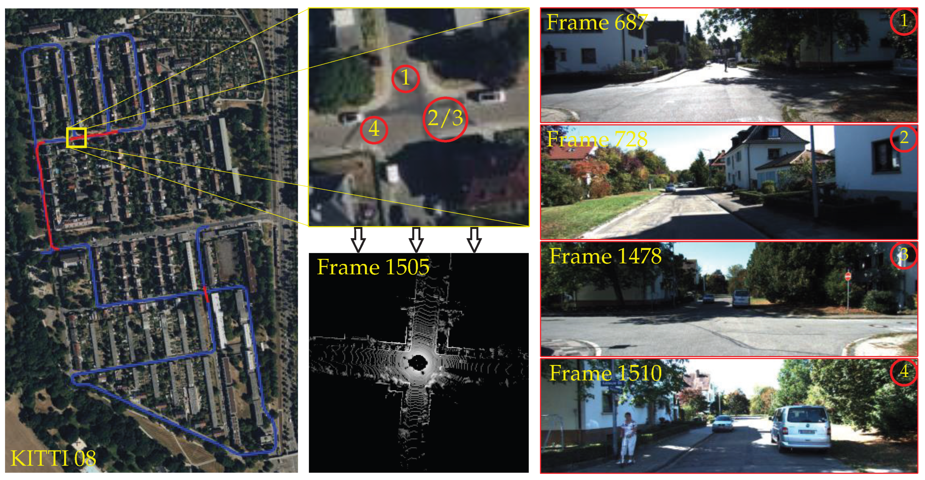
During vehicle operation, situations involving rotation—such as intersections and reverse revisits—are frequently encountered, as illustrated in Figure 1 for a particular intersection in Sequence 08 of the KITTI [2] dataset. Addressing the key challenge of rotation robustness, several researchers have conducted a series of studies, either through data augmentation or by designing rotation-invariant network architectures. Nevertheless, existing methods still face challenges in balancing accuracy and computational efficiency, suffer from discriminative degradation under extreme viewpoints, and exhibit limited generalization capability, which collectively hinder their deployment on resource-constrained autonomous driving platforms.

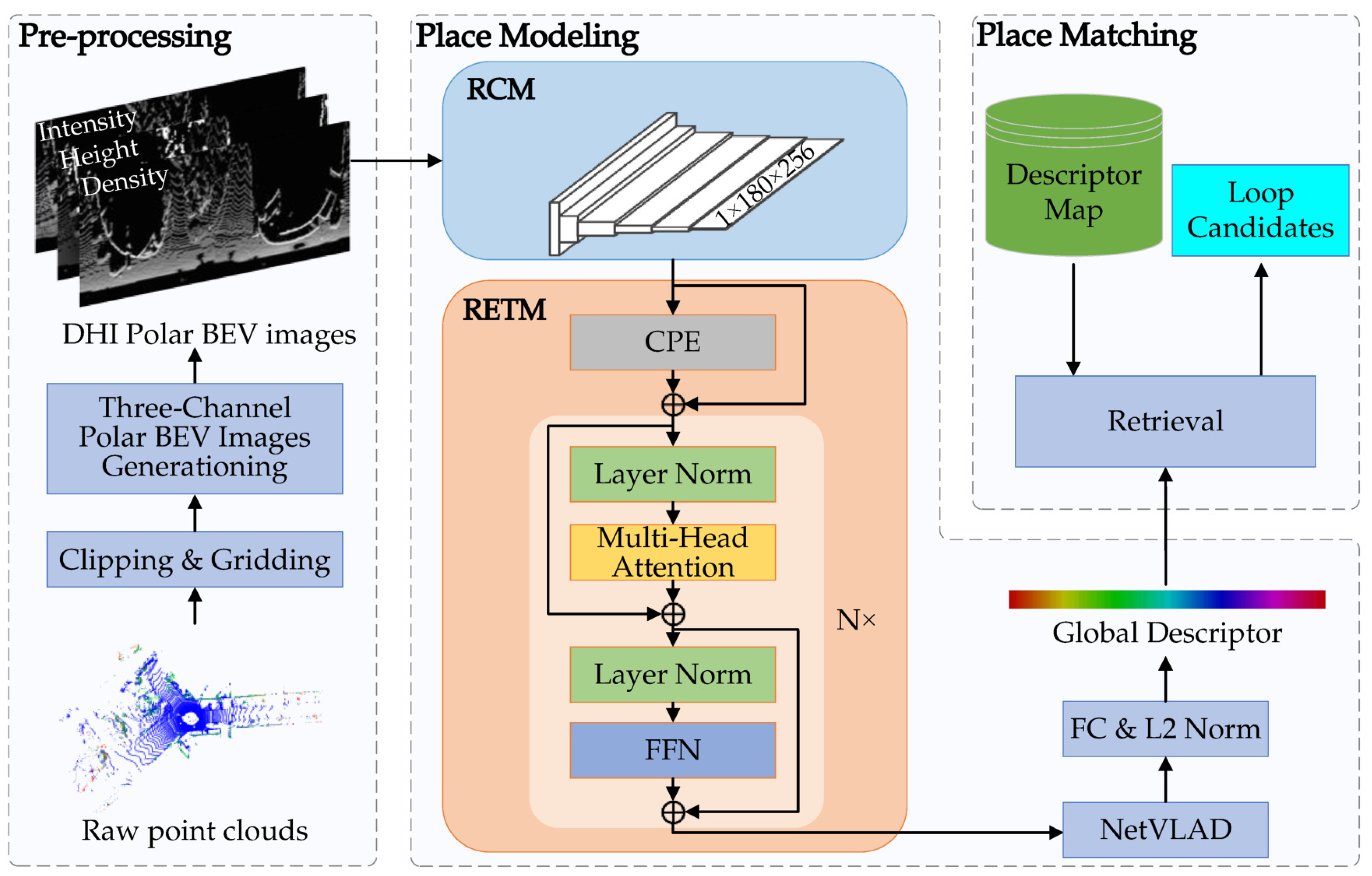
To address these limitations, this paper proposes a lightweight LiDAR place recognition framework that improves robustness to large yaw rotations. In the proposed method, the LiDAR point cloud is projected onto the horizontal plane and rasterized onto a polar grid. A three-channel polar BEV image is then constructed by encoding the point density, maximum height, and mean reflection intensity within each grid cell. To extract rotation-equivariant features from this representation, we design a rotation-equivariant feature encoder (REFE) comprising two key components: a Radial Compression Module (RCM) that aggregates radial information via axial-separable convolution with circular padding, and a rotation-equivariant Transformer module (RETM) that captures long-range azimuthal dependencies using Conditional Positional Encoding (CPE) and Circular Relative-Position Bias (CRPB). Subsequently, the resulting equivariant feature sequence is aggregated by NetVLAD into a global descriptor. The overall workflow of the proposed framework is illustrated in Figure 2, covering polar BEV generation, rotation-equivariant feature extraction, global descriptor aggregation, and descriptor-based place matching.

It should be noted that the novelty of the proposed method does not lie in using a polar grid, Transformer encoder, or NetVLAD aggregation in isolation, since these ideas have been explored in previous place recognition studies. Instead, the main novelty lies in coupling a multi-channel polar BEV representation with a rotation-equivariant feature encoder specifically designed for the cyclic-shift structure induced by yaw rotations. Compared with hand-crafted polar descriptors, such as Scan Context [3], our method learns compact descriptors end-to-end from density, height, and intensity cues. Compared with range-image-based methods, such as OverlapTransformer [4], the proposed framework preserves top-down BEV structural information while enforcing circular azimuthal equivariance throughout the feature extraction process.

The main contributions of this paper are summarized as follows:

1.

We propose a LiDAR place recognition framework based on a multi-channel polar BEV representation. By leveraging the polar BEV image, the vehicle’s yaw rotation is transformed into a cyclic shift in image columns, thereby converting the rotation invariance problem into a translation invariance problem and laying the foundation for the subsequent design of a rotation-equivariant feature extractor.

2.

We design a feature encoder comprising an RCM and an RETM. The RCM employs axial-separable convolutions to aggregate radial information while progressively compressing the radial dimension; the RETM leverages CPE and CRPB to capture long-range azimuthal dependencies, establishing global contextual associations without compromising rotation equivariance.

3.

We conduct extensive evaluations on the public KITTI and NCLT [5] datasets, as well as our self-constructed LiDAR Place Recognition Revisit (LPRR) dataset. The results demonstrate that the proposed method achieves competitive performance on KITTI and superior performance on NCLT and LPRR among the compared methods in terms of Recall@K and low computational overhead, and shows promising cross-dataset generalization on the evaluated NCLT and LPRR datasets without fine-tuning.

The remainder of this paper is organized as follows. Section 2 reviews existing LiDAR place recognition methods based on BEV images, range images, point clouds, and multi-modal representations. Section 3 presents the proposed methodology, including the construction of three-channel polar BEV images, the rotation-equivariant feature encoder, the global descriptor generator, and the training objective. Section 4 reports the experimental setup, quantitative comparisons, ablation studies, and runtime analysis on the KITTI, NCLT, and LPRR datasets. Section 5 concludes the paper and discusses the main findings.

2. Related Work

Depending on the data representation, existing LPR methods can be broadly divided into two categories: approaches based on 3D points [6,7,8] and approaches based on projection images. In this section, we briefly review recent advances in projection-image-based LPR, with a particular focus on algorithmic designs targeting rotation invariance. For a more comprehensive understanding of LPR, readers are referred to [1,9].

2.1. BEV Image-Based Methods

BEV images are obtained by orthographically projecting the point cloud onto the horizontal plane, discarding vertical height information while preserving the rigid geometric structures in the horizontal plane. This representation provides a holistic top-down view of the environment, facilitating the capture of static structures such as buildings and roads and their relative positional relationships, thereby enhancing the stability and repeatability of place recognition. BVMatch [10] uniformly discretizes the ground region, projects the point cloud onto the horizontal plane, counts the number of points within each grid cell, and normalizes the counts to produce a single-channel point cloud density image. A Log-Gabor filter is then applied to construct a maximum index map that encodes structural orientation information, yielding a descriptor insensitive to intensity and rotation variations. BEVPlace [11] employs group convolutions to extract rotation-equivariant local features, which are subsequently aggregated via NetVLAD [12] into rotation-invariant global features. BEVPlace++ [13] proposes a feature extraction pipeline for BEV images using both rotation-equivariant and rotation-invariant networks, with ResNet34 [14] as the backbone and a rotation-equivariant module to extract equivariant local features, followed by NetVLAD aggregation to generate rotation-invariant global descriptors. R2SCAT-LPR [15] projects point clouds into BEV images through random rotation augmentation, extracts multi-level patch features using cascaded multi-head self-attention mechanisms, and employs a dual-branch self- and cross-attention module to enhance the rotation robustness of the network. ForestLPR [16] slices the point cloud along the vertical direction to produce multi-height BEV density images and then applies a Transformer-based interaction module to obtain discriminative features from different heights. Scan Context [3] centers the LiDAR at its current pose and partitions the point cloud from a bird’s-eye perspective into sectors and rings according to azimuth and radial distance, encoding the maximum height within each bin into a matrix. To address translational sensitivity, the original point cloud is slightly shifted to multiple neighboring positions, and the resulting feature descriptors are stored. During query matching, the descriptor to be matched is compared against all shifted descriptors associated with that location in the database, thereby compensating for recognition errors induced by minor translations. Scan Context++ [17] improves upon Scan Context by proposing dual context descriptors in polar and Cartesian coordinates, tailored for rotational and lateral translational scenarios, respectively. By applying lateral shifts to the polar descriptor and bi-axial flips to the Cartesian descriptor, augmented descriptors are generated to accommodate composite motion scenarios.

2.2. Range Image-Based Methods

Range images—a range image is generated by spherically projecting the point cloud onto an image plane, where each pixel value corresponds to the distance from the LiDAR sensor to a point in the scene. This representation directly reflects the geometry of visible surfaces and inherently possesses rotation-equivariant properties. OverlapNet [18], as a representative work, innovatively introduces the concept of overlap from photogrammetry and computer vision into place recognition. It extracts multiple types of information from the point cloud—including depth, reflectivity, normal vectors, and semantics—and projects each modality via spherical projection to form a set of 2D images. These images are then compared against corresponding data in a database, and the similarity is computed based on the frame-to-frame overlap ratio, thereby achieving place recognition. OverlapTransformer [4] improves upon OverlapNet by relying solely on single-channel depth information to generate the range image, converting the similarity computation between point clouds into a descriptor matching problem. SeqOT [19] is a spatial-temporal Transformer-based framework designed for LiDAR sequence-based place recognition. Different from previous methods that process individual LiDAR scans independently, it takes consecutive range images as input and leverages two types of Transformer modules to jointly capture spatial and temporal cues from sequential LiDAR data. The single-scan Transformer extracts spatial features for each frame while retaining yaw-rotation equivariance, and the multiscan Transformer further models temporal correlations across three consecutive scans. By concatenating frame-wise features along the width dimension and adopting a simplified QKV design that keeps attention weights invariant to horizontal feature shifts, the method strictly preserves geometric properties during feature learning. CVT-Net [20] proposes a multi-layer projection of the point cloud at varying depths and heights, producing multi-layer depth maps and bird’s-eye views. The projected features are then compressed, aligned, and fused, ultimately yielding point cloud descriptors that are robust to viewpoint rotations. OverlapMamba [21] further advances OverlapTransformer by introducing the Mamba state-space model. By summing the SSM outputs of forward and reverse sequences, it ensures contextual integrity of the feature sequence under arbitrary yaw angles. During training, random cyclic shifts are employed to simulate different yaw angles, thereby enhancing the model’s ability to learn viewpoint-agnostic features.

To further clarify the characteristics of different LPR representations,

Table 1. Summary of representative LiDAR place recognition methods based on different data representations.

Category	Representative Methods	Advantages	Limitations
3D point-based methods	PointNetVLAD [6], LPD-Net [7], HOTFormerLoc [8]	Directly process raw point clouds and preserve original 3D geometric information.	Computationally expensive and rotation robustness usually depends on data augmentation, pose alignment, or specialized network designs.
BEV image-based methods	BVMatch [10], BEVPlace [11], BEVPlace++ [13], ForestLPR [16], Scan Context [3], Scan Context++ [17]	Provide compact BEV representations of point clouds and preserve horizontal structural layouts.	Cartesian BEV representations are highly sensitive to yaw rotations, often requiring data augmentation strategies to improve rotation robustness.
Range image-based methods	OverlapNet [18], OverlapTransformer [4], CVT-Net [20], OverlapMamba [21]	Generate range images via spherical projection of point clouds and naturally preserve rotation-equivariant properties.	Spherical projection may introduce scale variations and viewpoint-dependent distortions, affecting descriptor stability under large viewpoint changes.

summarizes representative methods, advantages, and limitations of the main categories discussed above.

As shown in Table 1, existing representations provide different trade-offs between geometric preservation, computational efficiency, and rotation robustness. These observations motivate the proposed polar BEV-based framework, which aims to preserve compact structural representation while explicitly improving yaw rotation robustness.

3. Methodology

This section elaborates on the proposed LiDAR place recognition method based on polar BEV representation and rotation-equivariant feature extraction. The overview of the proposed framework is depicted in Figure 2. First, the raw LiDAR point cloud is projected onto a polar grid. By aggregating the point count, maximum height, and mean intensity within each grid cell, a density-height-intensity (DHI) three-channel polar BEV image is constructed, achieving multi-attribute fusion encoding of the point cloud’s spatial distribution, geometric structure, and physical reflection properties (Section 3.1). Subsequently, to meet the rotation equivariance requirement of the polar BEV image, a rotation-equivariant feature extractor (REFE) is designed, comprising a Radial Compression Module (RCM) and a rotation-equivariant Transformer module (RETM). The RCM progressively compresses the radial dimension via axial-separable convolution, outputting a feature sequence along the azimuthal direction. The RETM establishes long-range azimuthal correlations while preserving rotation equivariance by employing Conditional Positional Encoding (CPE) and Circular Relative-Position Bias (CRPB) (Section 3.2). Next, the equivariant azimuthal feature sequence is fed into a Global Descriptor Generator (GDG), where NetVLAD aggregates it into a compact global descriptor with improved robustness to yaw rotations (Section 3.3). Finally, a hard sample mining triplet loss is adopted to train the network, thereby enhancing feature discriminability (Section 3.4).

3.1. Generation of Three-Channel Polar BEV Images

In this paper, we assume that the vehicle operates on structured paved road surfaces, such as urban roads and highways, which are approximately planar within a local region. Conventional BEV images are obtained by orthogonally projecting the LiDAR point cloud onto a Cartesian grid representation. Although such a representation preserves the global scene structure from a real-world perspective, it is inherently sensitive to variations in the vehicle’s yaw angle, manifesting as a global rotation of the BEV image and consequently increasing the difficulty of subsequent feature encoding and retrieval.

To enhance robustness against yaw-angle variations, we adopt a polar BEV representation. In this representation, the three-dimensional LiDAR point cloud is vertically projected onto the horizontal plane via BEV orthogonal projection, and the ground plane is partitioned into grid cells along the radial and azimuthal directions. The radial resolution $N_r$ corresponds to the number of rows in the image, while the azimuthal resolution $N_{\theta }$ corresponds to the number of columns, with each grid cell serving as a pixel of the polar BEV image.

We adopt the vehicle body coordinate system as the reference frame, in which the X-axis points forward, the Y-axis points leftward, and the Z-axis points upward. In this system, the $XY$-plane coincides with the ground plane. Let the point cloud acquired by the LiDAR at time t be denoted as

$${\mathcal{P}}_t=\{p_j\mid j=1,\dots ,N_t\},p_j=(x_j,y_j,z_j,i_j).$$

(1)

where $p_j=(x_j,y_j,z_j,i_j)$ represents the three-dimensional coordinates and reflection intensity of the j-th point, and $N_t$ is the total number of points in the cloud.

To focus on the effective sensing range and to remove noisy points, we crop the point cloud to a cylindrical region of radius $r_{max}$ centered at the vehicle and restrict the height within the interval $[z_{min},z_{max}]$. Specifically, the cropped point cloud is defined as

$${\mathcal{P}}_t^{\prime }=\left\{p_j\in {\mathcal{P}}_t\mid \sqrt{x_j^2+y_j^2}\le r_{max},z_{min}\le z_j\le z_{max}\right\}$$

(2)

Subsequently, the cropped point cloud is processed via polar grid binning to generate the polar BEV image. Specifically, the radial interval $[0,r_{max}]$ is uniformly divided into $N_r$ bins, where $r_{max}$ denotes the maximum sensing distance and the radial resolution is defined as $\Delta r=r_{max}/N_r$; the azimuthal interval $[0,2\pi )$ is uniformly divided into $N_{\theta }$ sectors, yielding an azimuthal resolution of $\Delta \theta =2\pi /N_{\theta }$. This yields a set of polar grid cells $\left\{{\mathcal{G}}_{r,\theta }\right\}$, each corresponding to a fan-shaped region:

$${\mathcal{G}}_{r,\theta }=\{(x,y)\in {\mathbb{R}}^2\mid r\le \sqrt{x^2+y^2}<r+\Delta r,\theta \le atan2(y,x)<\theta +\Delta \theta \}$$

(3)

For each grid cell $(r,\theta )$, the LiDAR points falling within it are aggregated, and three-channel features—namely point density, maximum height, and mean intensity—are computed, thereby constructing a DHI three-channel polar BEV image.

Density channel. The number of points $n_{(r,\theta )}$ within a grid cell $(r,\theta )$ is counted, then subjected to a logarithmic transformation and normalized as follows:

$$D(r,\theta )={\displaystyle \frac{ln\left(1+min\left(n_{(r,\theta )},n_{99}\right)\right)}{ln\left(1+n_{99}\right)}}$$

(4)

where $n_{99}$ is the 99th percentile of the point counts across grid cells.

Maximum height channel. Within each grid cell $(r,\theta )$, the relative height is defined as the maximum vertical offset of the point cloud with respect to the lower height bound $z_{min}$:

$$h(r,\theta )=\underset{p_i\in {\mathcal{P}}_t^{\prime }}{max}\left(z_i-z_{min}\right)$$

(5)

This value is then normalized as

$$H(r,\theta )={\displaystyle \frac{min\left(h(r,\theta ),h_{99}\right)}{h_{99}}}$$

(6)

where $h_{99}$ denotes the 99-th percentile of the maximum heights over all grid cells.

Mean intensity channel. The mean reflection intensity of points within grid cell $(r,\theta )$ is computed as ${\overline{i}}_{(r,\theta )}$ and then normalized:

$$I(r,\theta )={\displaystyle \frac{{\overline{i}}_{(r,\theta )}}{{max}_{(r^{\prime },{\theta }^{\prime })\in \left\{{\mathcal{G}}_{r,\theta }\right\}}\left({\overline{i}}_{(r^{\prime },{\theta }^{\prime })}\right)}}$$

(7)

If a grid cell contains no LiDAR points, the density, maximum height, and mean intensity channels for that cell are set to zero.

Finally, the three channels $D(r,\theta )$, $H(r,\theta )$, and $I(r,\theta )$ are combined to form a DHI three-channel polar BEV image representation.

3.2. Rotation-Equivariant Feature Extraction

After encoding the LiDAR point cloud into a DHI three-channel polar BEV image, it is necessary to further extract local features to obtain a spatially structured feature representation $\mathbf{F}$ that is both discriminative and rotation-equivariant. In this paper, we design a REFE tailored to the polar BEV image for feature extraction. Specifically, the REFE consists of an RCM followed by a Transformer encoder. The RCM progressively compresses the radial dimension to one, yielding a feature sequence of length $N_{\theta }$, and the Transformer encoder then models global relationships across this sequence to capture long-range azimuthal correlations.

It should be noted that this cyclic-shift relationship strictly holds under an ideal yaw-only transformation, where the LiDAR observes the same place from approximately the same sensor center and the dominant change is the heading angle. In practical revisits, lateral translation, viewpoint-dependent occlusion, dynamic objects, non-planar terrain, and changes in visible scene content may violate this assumption. Therefore, the proposed representation should be understood as providing a structural prior for improving rotation robustness rather than guaranteeing perfect rotation invariance in all real-world scenarios.

3.2.1. Radial Compression Module

In the polar BEV representation, a change in the vehicle’s heading at a fixed position alters only the azimuthal coordinates in the polar BEV image, without affecting the radial distances. Owing to the periodicity of the azimuth angle, $\theta$ and $\theta +2\pi$ correspond to the same direction. When the vehicle undergoes a counterclockwise yaw rotation by $\Delta \psi$, a scene point originally at azimuth $\theta$ shifts to $\theta -\Delta \psi$. In the polar BEV image, this yaw rotation manifests as a leftward integer shift of $k=\lfloor \Delta \psi ·N_{\theta }/2\pi \rfloor$ columns along the azimuthal direction.

The RCM consists of multiple stacked convolutional layers. The core idea is to progressively reduce the radial resolution while increasing the number of channels, keeping the azimuthal dimension unchanged. The input image has dimensions $N_r=100$ and $N_{\theta }=180$. The RCM transforms the input from $N_r\times N_{\theta }\times 3$ to $1\times N_{\theta }\times C$.

To reduce computational cost while preserving directional geometric priors, we decouple the standard 2D convolution into sequential 1D convolutions along the radial and azimuthal axes, respectively. We term this design axis-wise separable convolution. Along the radial dimension, zero padding is applied to progressively aggregate distance information; along the azimuthal dimension, circular padding is adopted to preserve equivariance to cyclic azimuthal shifts under the yaw-only assumption.

The RCM adopts a stage-wise homogeneous encoding strategy. Stages 1–3 form a shallow geometric encoder that employs $3\times 3$ axial-separable convolutions to rapidly reduce resolution and expand the channel count, extracting initial features. Stages 4–6 constitute a deep semantic compressor that uses a bottleneck structure to further compress the radial dimension while maintaining the channel count $C=256$, refining the high-dimensional features. The final output is a feature map consisting of $N_{\theta }$ feature vectors along the azimuthal direction. This two-stage design conforms to the general principle of visual representation learning, transitioning from shallow detail features to deep abstract features, and the structured design facilitates gradient propagation and optimization stability. The architecture of the RCM is detailed in

Table 2. Network architecture of the Radial Compression Module (RCM).

Layer	Kernel Size	Stride	Filter	Output Shape
Stage 1	$3\times 3$	$(2,1)$	64	$50\times 180\times 64$
Stage 2	$3\times 3$	$(2,1)$	128	$25\times 180\times 128$
Stage 3	$3\times 3$	$(2,1)$	256	$13\times 180\times 256$
Stage 4	$1\times 1$	$(1,1)$	64	$7\times 180\times 256$
	$3\times 3$	$(2,1)$	64
	$1\times 1$	$(1,1)$	256
Stage 5	$1\times 1$	$(1,1)$	64	$4\times 180\times 256$
	$3\times 3$	$(2,1)$	64
	$1\times 1$	$(1,1)$	256
Stage 6	$1\times 1$	$(1,1)$	64	$1\times 180\times 256$
	$3\times 3$	$(2,1)$	64
	$1\times 1$	$(1,1)$	256

.

3.2.2. Rotation-Equivariant Transformer Module

The RCM removes the radial dimension from the polar BEV image $\mathcal{I}\in {\mathbb{R}}^{N_r\times N_{\theta }\times 3}$ to obtain a compact feature sequence of length $N_{\theta }$ along the azimuthal direction, denoted as ${\mathbf{F}}_{\mathrm{RCM}}\in {\mathbb{R}}^{1\times N_{\theta }\times C}$. The output of the RCM is then reshaped into a sequence $\mathbf{S}={\left\{{\mathbf{s}}_i\right\}}_{i=1}^{N_{\theta }}\in {\mathbb{R}}^{N_{\theta }\times C}$, where ${\mathbf{s}}_i\in {\mathbb{R}}^C$ is the feature vector at the i-th azimuth, and ${\mathbf{s}}_i$ already aggregates the local contextual information of that direction and its neighboring sectors. To establish correlations between distant azimuthal positions, we design an RETM that explicitly incorporates the cyclic topology of the azimuthal sequence into the self-attention mechanism.

In conventional Transformer architectures [22], positional encodings, whether absolute or relative, lack periodic constraints on the position indices and therefore do not satisfy circular consistency along the azimuthal dimension. To ensure rotation equivariance of the network module, we adopt CPE [23] based on depthwise separable convolution. This method performs 1D convolution along the azimuthal dimension to dynamically generate a position-aware representation from the input feature sequence, thereby establishing locally position-aware correlations with rotation equivariance for each azimuthal token.

The core idea of Conditional Positional Encoding is to use the convolution result along the azimuthal direction as the positional encoding information, decoupling spatial mixing from channel mixing. Specifically, for the input azimuthal feature sequence $\mathbf{S}$, the positional encoding is obtained through two steps: depthwise convolution and pointwise convolution.

First, a depthwise convolution applies a 1D convolution independently to each channel along the azimuthal dimension to establish local spatial relationships. To ensure rotation equivariance, a circular padding strategy is adopted along the azimuthal dimension. Then, a pointwise convolution performs linear mixing along the channel dimension to enable cross-channel interaction. The pointwise convolution operates independently at each individual azimuthal position using a $1\times 1$ convolution, without introducing cross-position spatial mixing, thus preserving the sequence length. The resulting positional encoding is denoted as ${\mathbf{P}}_{\mathrm{CPE}}\in {\mathbb{R}}^{N_{\theta }\times C}$.

The output of the CPE has the same dimensions $N_{\theta }\times C$ as the input feature sequence. Adding it to the input yields the position-augmented features:

$${\mathbf{s}}_i^{\prime }={\mathbf{s}}_i+{\mathbf{P}}_{\mathrm{CPE}}\left(i\right)$$

(8)

where ${\mathbf{P}}_{\mathrm{CPE}}\left(i\right)\in {\mathbb{R}}^C$ denotes the positional encoding vector at azimuthal position i, and ${\mathbf{s}}_i^{\prime }$ denotes the input feature augmented with azimuthal positional information. Owing to the translation equivariance of convolution, this encoding naturally satisfies cyclic shift equivariance: when the entire sequence is shifted as a whole, the relative positional encoding remains unchanged, thereby ensuring the stability of the attention weight distribution.

Building upon multi-head self-attention, we introduce a CRPB to address the lack of azimuthal geometric awareness. A learnable bias term ${\mathbf{B}}_{(j-i)mod{N}_{\theta }}$ is employed to explicitly model the circular relative distance between tokens. For the i-th azimuthal token attending to all tokens, the attention score is computed as

$$\mathrm{Attention}(Q,K,V)=\mathrm{softmax}\left({\displaystyle \frac{Q{K}^T}{\sqrt{d_k}}}+{\mathbf{B}}_{(j-i)mod{N}_{\theta }}\right)V$$

(9)

where ${\mathbf{B}}_{(j-i)mod{N}_{\theta }}\in {\mathbb{R}}^{N_{\theta }}$ is a learnable Relative-Position-Bias vector that depends only on the circular distance $(j-i)mod{N}_{\theta }$ between tokens. When the entire sequence is shifted, $(j-i)mod{N}_{\theta }$ remains invariant; consequently, the attention map remains consistent under cyclic shifts, and the network preserves rotation equivariance.

We adopt a Pre-Layer Normalization (Pre LN) architecture and is stacked with L identical encoder layers. Each encoder layer consists of two sublayers: multi-head self-attention (MHSA) and a feed-forward network (FFN), formulated as

$$X_{l+1}=X_l+\mathrm{Sublayer}\left(\mathrm{LN}\left(X_l\right)\right)$$

(10)

The MHSA employs $N_{\mathrm{head}}$ attention heads and leverages the CRPB mechanism to model circular dependencies among azimuthal tokens. The FFN comprises two fully connected layers with an intermediate dimension expanded to $4C$, using the GELU activation function. To maintain rotation equivariance under cyclic azimuthal shifts, the FFN operates independently on each token along the azimuthal dimension in a pointwise manner, without introducing cross-position spatial convolutions or fully connected operations.

3.3. Global Descriptor Generator

After processing by the RETM, we obtain a feature sequence $F_{\mathrm{trans}}\in {\mathbb{R}}^{N_{\theta }\times C}$ encoded along the azimuthal dimension. This feature sequence is rotation-equivariant. However, place recognition tasks benefit from global descriptors that are robust to yaw-induced cyclic shifts.

In this paper, we adopt NetVLAD as the global descriptor generator. NetVLAD is an aggregation layer widely used in visual place recognition tasks. Unlike its original design tailored for two-dimensional CNN feature maps, we apply NetVLAD to the one-dimensional azimuthal feature sequence $F_{\mathrm{trans}}\in {\mathbb{R}}^{N_{\theta }\times C}$ derived from the polar BEV image, where the feature vector at each azimuthal position is treated as a local descriptor for cluster-based aggregation:

$$v_m={\displaystyle \sum _{i=1}^{N_{\theta }}}{w}_{im}\left(f_i-c_m\right)$$

(11)

where $v_m$ is the VLAD residual vector for cluster m, $w_{im}$ are soft-assignment weights, $f_i$ is the feature at position i, and $c_m$ is the centroid of cluster m. Concatenating the residual vectors ${\left\{v_m\right\}}_{m=1}^M$ of all M clusters yields a VLAD vector of dimension $M·C$, which is subsequently projected to $D_{\mathrm{out}}=256$ dimensions via a fully connected (FC) layer and L2-normalized to yield the final yaw-rotation-robust global descriptor.

3.4. Network Training

We train the proposed network in an end-to-end manner. For an input point cloud ${\mathcal{P}}_t$, its corresponding global descriptor is denoted as $g_t\in {\mathbb{R}}^{M·C}$. In this paper, we adopt a hard sample mining triplet loss for network optimization.

For each training batch, j locations are randomly selected, and from each location, m point cloud frames are randomly sampled to generate global descriptors, yielding a total of $j·m$ samples in a batch. Based on the ground-truth global poses of the point clouds, the translational distances between point clouds are computed. For a given anchor sample ${\mathcal{P}}_{\mathrm{anchor}}$ in the batch, point clouds whose pose translation distance is smaller than the positive threshold ${\tau }_{\mathrm{pos}}$ are assigned to the same-location set $\left\{{\mathcal{P}}_{\mathrm{pos}}\right\}$, while those with a translation distance larger than the negative threshold ${\tau }_{\mathrm{neg}}$ are assigned to the different-location set $\left\{{\mathcal{P}}_{\mathrm{neg}}\right\}$.

As the global descriptors are L2-normalized, we adopt the cosine distance to measure the spatial similarity of the global features. We then select the hardest positive sample ${\mathcal{P}}_{\mathrm{pos}}^{+}$ and the hardest negative sample ${\mathcal{P}}_{\mathrm{neg}}^{-}$ to form a triplet. The loss function is formulated as

$$\mathcal{L}={\displaystyle \frac{1}{j·m}}\sum _{{\mathcal{P}}_{\mathrm{anchor}}\in \mathrm{Batch}}{\left[\underset{\mathcal{P}\in \left\{{\mathcal{P}}_{\mathrm{pos}}\right\}}{max}\left(1-\langle f\left({\mathcal{P}}_{\mathrm{anchor}}\right),f\left(\mathcal{P}\right)\rangle \right)-\underset{\mathcal{P}\in \left\{{\mathcal{P}}_{\mathrm{neg}}\right\}}{min}\left(1-\langle f\left({\mathcal{P}}_{\mathrm{anchor}}\right),f\left(\mathcal{P}\right)\rangle \right)+\beta \right]}_{+}$$

(12)

where $\beta$ is a constant hyperparameter that defines the margin, ${[\dots ]}_{+}$ denotes the hinge loss, and $\langle ·,·\rangle$ represents the vector inner product.

In summary, this section presents the complete methodology of the proposed LPR framework. The raw point cloud is first converted into a DHI polar BEV representation, where yaw rotations are transformed into cyclic shifts along the azimuthal dimension. Based on this representation, the proposed REFE extracts rotation-equivariant features through radial compression and azimuthal contextual modeling. Finally, NetVLAD aggregates the equivariant feature sequence into a compact rotation-invariant global descriptor, and the network is optimized using a hard sample mining triplet loss.

4. Evaluation Setup

This section presents the experimental setup, including the datasets employed and the evaluation metrics used to assess place recognition performance.

4.1. Datasets

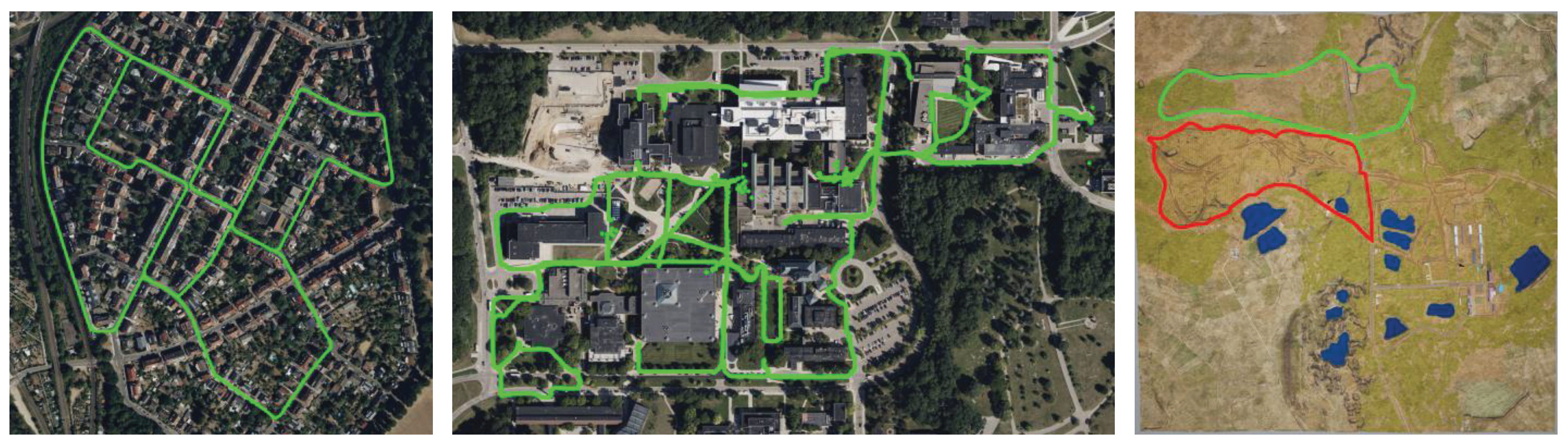
In this paper, three datasets are adopted to evaluate the performance of the proposed method for the place recognition task. The first consists of the widely used public datasets KITTI and NCLT, which are employed to assess the overall performance of the algorithm. The second is a self-constructed dataset based on the Car Learning to Act (CARLA) simulation platform [24], specifically designed for evaluating robustness to large yaw rotations, and is used to evaluate the algorithm’s performance under rotational conditions. The trajectories of the three dataset sequences used in this paper are shown in Figure 3 on satellite maps.

KITTI dataset. As one of the most representative public datasets in autonomous driving, KITTI provides real-world road scene data collected by vehicle-mounted sensors. In this paper, we conduct experiments using the KITTI Odometry Benchmark sequences. Specifically, sequences 03 to 10 are used for network training, sequence 02 for validation, and sequence 00 for testing, with frames 0 to 3000 employed to construct the database, and frames 3200 to 4541 used for queries.

NCLT dataset. This dataset is an important resource for studying long-term autonomous robot operation. Data were collected at the University of Michigan, encompassing multiple repeated trajectories in a campus environment. The NCLT dataset spans multiple months with varying weather and vegetation conditions, making it ideal for evaluating cross-session robustness. In this paper, we select two representative sequences for experiments: sequence 2012-01-08 is used to construct the database, and sequence 2012-02-05 is used for queries.

Self-constructed LiDAR Place Recognition Revisit (LPRR) dataset. Although public LiDAR datasets such as KITTI and NCLT provide a real-world scene foundation for place recognition research, they suffer from notable limitations in terms of coverage density of vehicle revisit scenarios and the controllability of rotation angles. Specifically, real-world data collection makes it difficult to systematically introduce substantial heading variations while ensuring strictly overlapped trajectories, which in turn hinders the disentanglement of pose error interference and prevents targeted evaluation of algorithmic robustness to rotational changes. To address this shortcoming, we construct a supplementary dataset specifically designed for rotation-robustness validation using the CARLA open-source autonomous driving simulation platform.

To clarify the hardware and software implementation of the self-constructed dataset, the simulation platform, sensor configuration, and data acquisition pipeline are described as follows. A real-world off-road area of approximately $2\mathrm{km}\times 2\mathrm{km}$ is modeled as a custom simulation map using Unreal Engine 4. The data acquisition software is implemented using the Python API provided by CARLA 0.9.14, which is used for vehicle control, sensor configuration, data synchronization, and ground-truth pose recording. The simulator adopts a left-handed coordinate system in which the +X axis points forward along the driving direction, the +Y axis points to the right of the vehicle, and the +Z axis points vertically upward. The extrinsic matrices of all sensors and the ground-truth global poses are provided by the CARLA simulator API carla.Transform and follow this convention.

The virtual hardware configuration includes a LiDAR sensor and a forward-looking RGB camera mounted on the autonomous vehicle. The LiDAR is mounted on the vehicle roof to acquire three-dimensional point cloud data of the surrounding environment. Its specifications are as follows: vertical field of view ranging from −25° to +15°, horizontal field of view of 360°, 128 channels, and a point frequency of 1 MHz. Point cloud data are saved in PCD format, with an average size of approximately 2.1 MB per frame. The camera is mounted on the front part of the vehicle roof to capture RGB images of the environment ahead. Its specifications are as follows: image resolution of $800\times 800$ pixels, a horizontal field of view of 120°, and a frame rate of 10 Hz. Image data are saved in PNG format, with an average size of approximately 0.9 MB per frame.

Based on the above hardware and software configuration, we performed data acquisition by driving back and forth along two routes in the simulation scenario: one paved road and one dirt road. LiDAR point clouds, forward-looking camera images, and vehicle global poses were synchronously saved at intervals of 0.1 s, resulting in a total of four data sequences, as presented in

Table 3. Specifications of the sequences in the self-constructed LiDAR Place Recognition Revisit (LPRR) dataset.

Sequence	Length	Frame	Direction	Role
1-1	2.85 km	8628	clockwise	Database
1-2	2.91 km	8810	counterclockwise	Query
2-1	3.05 km	9120	clockwise	Database
2-2	3.07 km	9174	counterclockwise	Query

.

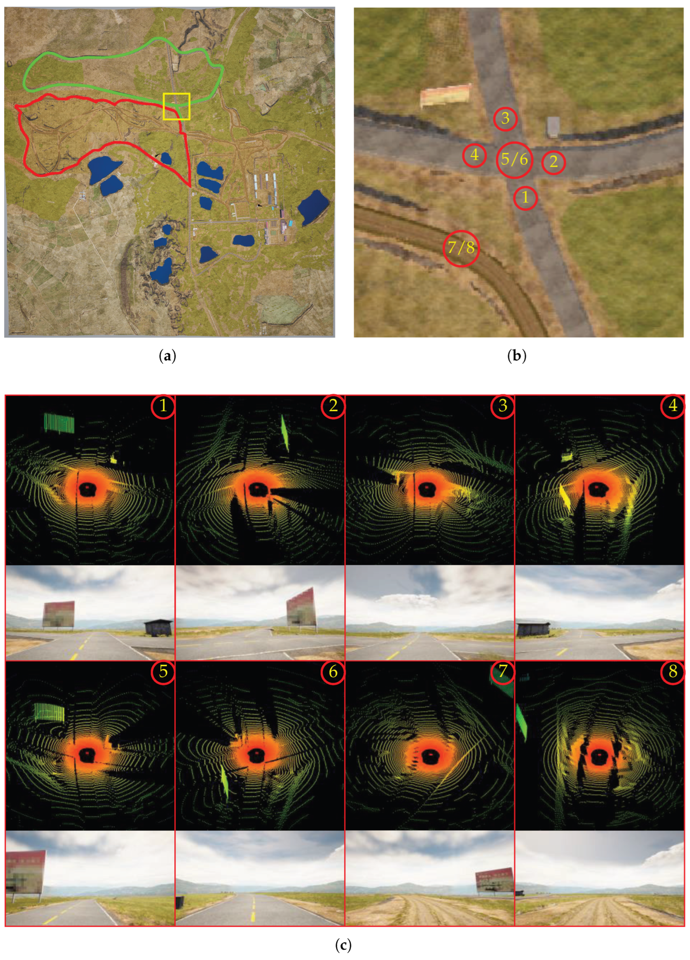
As illustrated in Figure 4, the LiDAR point clouds and camera images captured at different headings of the vehicle at a certain intersection in the simulation scenario exhibit notable appearance differences. Although these acquisition positions are spatially close to each other, the differing orientations lead to substantial variations in the LiDAR point clouds, which poses a significant challenge for place recognition.

4.2. Evaluation Metrics

To evaluate the place recognition performance of the proposed algorithm, we adopt Recall@K as the primary evaluation metric. This metric measures whether, for a given query frame, at least one true match exists among the top-K most similar candidates returned from the database. A successful place recognition is counted if such a match is found. The formula for Recall@K is given as follows:

$$\mathrm{Recall}@\mathrm{K}={\displaystyle \frac{1}{N_q}}{\displaystyle \sum _{i=1}^{N_q}}\mathbb{I}\left(\underset{p\in {\mathcal{T}}_K}{min}\mathcal{D}(p,{\mathcal{P}}_t)<\tau \right)$$

(13)

where $N_q$ is the total number of query samples, $\mathbb{I}(·)$ denotes the indicator function, ${\mathcal{T}}_K$ represents the set of the top-K retrieval results returned for the query point cloud ${\mathcal{P}}_t$ based on feature similarity, $\mathcal{D}(p,{\mathcal{P}}_t)$ is the Euclidean distance in pose space between the query point cloud ${\mathcal{P}}_t$ and a retrieved point cloud p, and $\tau$ is a distance threshold for determining whether two point clouds correspond to the same location.

In addition to Recall@K, we further report a top-1 threshold-based precision-recall (PR) curve as a threshold-based complementary evaluation. It should be noted that Recall@K differs from the recall used here. Recall@K is a ranking-based retrieval metric that evaluates whether at least one true match appears among the top-K retrieval candidates for each query. In contrast, the top-1 threshold PR curve evaluates, under varying descriptor distance thresholds, whether the retrieved top-1 candidate can be correctly accepted or rejected.

For each query, we first retrieve its top-1 database candidate according to descriptor distance, forming a query-candidate pair. Let $d_{\mathrm{desc}}$ denote the descriptor distance between the query and its top-1 candidate, and let $d_{\mathrm{pose}}$ denote their Euclidean pose distance. Given a descriptor-distance threshold $\delta$, the pair is predicted as positive if $d_{\mathrm{desc}}\le \delta$, and negative otherwise. The ground-truth label of the pair is positive if $d_{\mathrm{pose}}\le \tau$, where $\tau$ is the same place recognition distance threshold used in Recall@K; otherwise, it is negative.

Based on these binary decisions, true positives ($TP$), false positives ($FP$), false negatives ($FN$), and true negatives ($TN$) are counted as follows: $TP$ denotes accepted pairs that are ground-truth positives; $FP$ denotes accepted pairs that are ground-truth negatives; $FN$ denotes rejected pairs that are ground-truth positives; and $TN$ denotes rejected pairs that are ground-truth negatives. Precision and recall are then computed as

$$\mathrm{Precision}\left(\delta \right)={\displaystyle \frac{TP\left(\delta \right)}{TP\left(\delta \right)+FP\left(\delta \right)}},$$

(14)

$$\mathrm{Recall}\left(\delta \right)={\displaystyle \frac{TP\left(\delta \right)}{TP\left(\delta \right)+FN\left(\delta \right)}}.$$

(15)

By sweeping $\delta$, the PR curve characterizes the trade-off between accepting correct top-1 matches and suppressing incorrect top-1 matches.

5. Experimental Evaluation

This section presents extensive experiments to validate the place recognition performance of the proposed method on both public and self-constructed datasets. First, the network implementation details and key hyperparameter settings used during training are provided. Subsequently, quantitative comparisons between the proposed method and state-of-the-art approaches are reported. Ablation studies are then conducted to verify the effectiveness of the designed modules. Finally, the inference time and computational efficiency of the model are analyzed.

5.1. Implementation Details

Polar BEV Generation. The raw LiDAR point cloud is cropped to retain valid points within a cylindrical region centered at the vehicle with a radius of $r_{max}=40\mathrm{m}$ and a height range of $[z_{min},z_{max}]=[-5\mathrm{m},10\mathrm{m}]$. The cropped point cloud is then projected onto a polar grid, where each grid cell encodes three channels of information: density, maximum height, and mean intensity, ultimately generating a DHI polar BEV image of size $100\times 180\times 3$.

Network Architecture. In the proposed REFE, the detailed configuration of the RCM is provided in Table 1. The RCM progressively compresses the input spatial dimensions from $100\times 180\times 3$ to $1\times 180\times 256$ over six stages, outputting a feature sequence along the azimuthal direction. The RETM is stacked with $L=4$ encoder layers, where the number of heads in the MHSA is $N_{\mathrm{head}}=8$, and the intermediate dimension of the FFN is expanded to $4C=1024$. The number of cluster centers in NetVLAD is $M=64$, and the dimension of the final global descriptor after dimensionality reduction is $D_{\mathrm{out}}=256$.

Training Configuration. The network is trained end-to-end using the Adam optimizer with an initial learning rate of ${10}^{-4}$ and a weight decay coefficient of ${10}^{-4}$. The learning rate is scheduled via a cosine annealing strategy. Training is conducted for 200 epochs with a batch size of 16, i.e., randomly selecting $j=4$ locations per iteration and $m=4$ point cloud frames per location. The margin hyperparameter $\beta$ in the triplet loss is set to $0.5$. The positive threshold ${\tau }_{\mathrm{pos}}$ and negative threshold ${\tau }_{\mathrm{neg}}$ are set to $5\mathrm{m}$ and $10\mathrm{m}$, respectively. The proposed network is trained only on the KITTI dataset, using sequences 03–10 for training and sequence 02 for validation. The final in-domain test is conducted on KITTI sequence 00, where frames 0–3000 are used as the database and frames 3200–4541 are used as queries. The NCLT and LPRR datasets are not used for training or fine-tuning; they are used only for evaluation to assess cross-dataset generalization and robustness under different revisit conditions.

Retrieval. To ensure real-time place recognition, an approximate nearest neighbor search algorithm based on the Hierarchical Navigable Small World (HNSW) [25] graph is adopted for efficient matching of global descriptors during the retrieval stage. In our experiments, the HNSW algorithm uses the following parameters: number of neighbors per element is $M_{\mathrm{hnsw}}=16$, candidate list size during construction is $efConstruction=100$, and candidate list size during search is $ef=100$.

Baseline Evaluation. For the compared learning-based methods, including HOTFormerLoc [8], BEVPlace++ [13], and OverlapTransformer [4], we use the publicly available implementations and pretrained weights provided by the original authors. These methods are not retrained in our experiments. Instead, their pretrained models are directly used for descriptor extraction, and the extracted descriptors are evaluated on the dataset splits specified in this paper. For Scan Context [3], which is a hand-crafted descriptor rather than a deep learning model, no training is required; we evaluate it using the same database/query splits and matching protocol.

Hardware Environment. All experiments are performed on a workstation running Ubuntu 20.04, equipped with an Intel Core i7 12700K processor (3.6 GHz), 64 GB of RAM, an NVIDIA GeForce RTX 4090 D GPU (24 GB VRAM), and CUDA 12.1.

5.2. Evaluation for Place Recognition

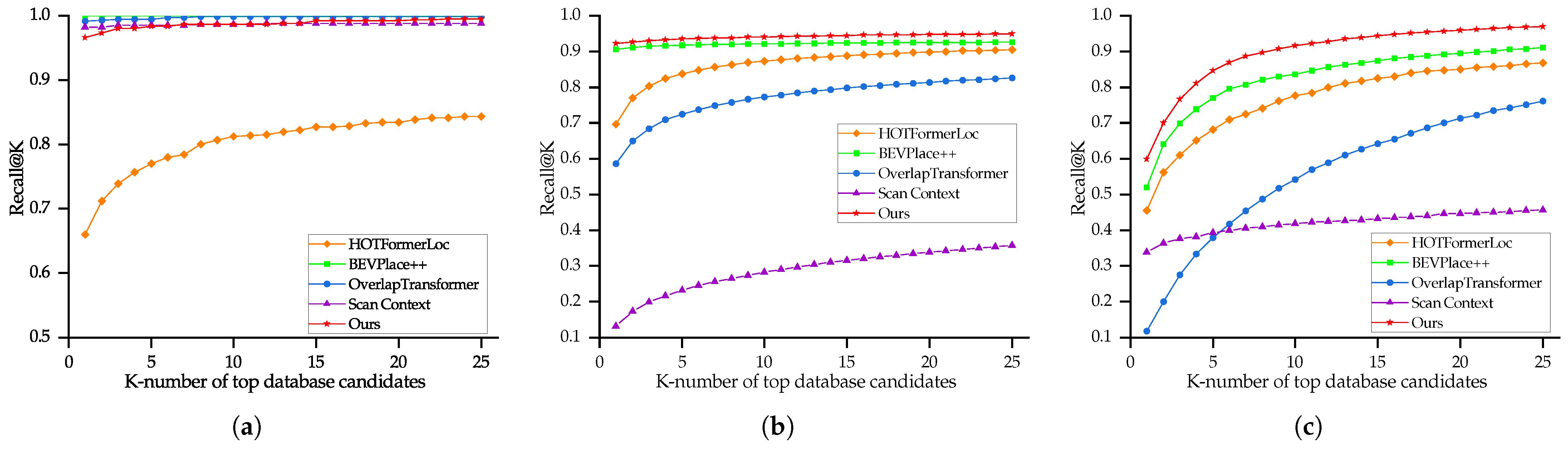
We compare the proposed method with HOTFormerLoc [8], BEVPlace++ [13], OverlapTransformer [4], and Scan Context [3] on the KITTI, NCLT, and LPRR datasets. The resulting Recall@K curves are presented in Figure 5 and Figure 6, and the quantitative comparison of the key metrics Recall@1 and Recall@25 is provided in

Table 4. Quantitative comparison of Recall@1 and Recall@25 of different algorithms.

Algorithm	Recall@1			Recall@25
	KITTI	NCLT	LPRR	KITTI	NCLT	LPRR
HOTFormerLoc	0.660	0.697	0.456	0.843	0.905	0.868
BEVPlace++	1.000	0.907	0.520	1.000	0.926	0.911
OverlapTransformer	0.991	0.586	0.117	0.999	0.826	0.761
Scan Context	0.982	0.131	0.339	0.988	0.357	0.457
Ours	0.966	0.923	0.599	0.995	0.949	0.970

.

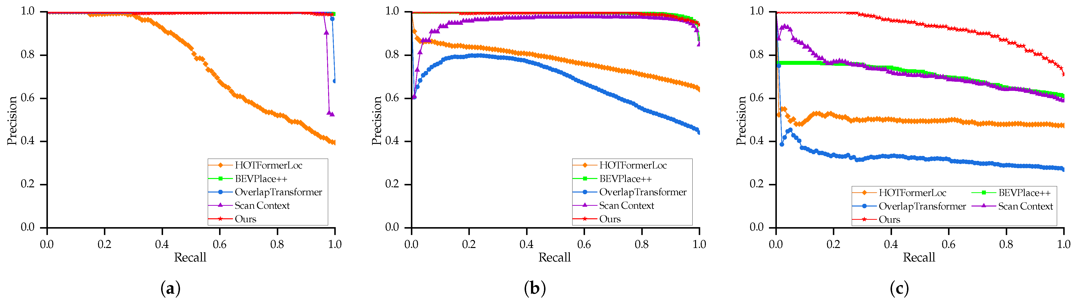
Results on the KITTI Dataset. Since the model is trained on other KITTI sequences and tested on sequence 00, this experiment mainly reflects in-domain performance under the KITTI odometry setting. Figure 5a presents the Recall@K curves of different algorithms on sequence 00 of the KITTI dataset. Overall, most learning-based methods achieve nearly saturated Recall@K performance on this dataset, indicating that KITTI sequence 00 is relatively less challenging when the training and testing data come from the same benchmark domain. BEVPlace++ achieves the best performance on KITTI, with both Recall@1 and Recall@25 reaching 1.000. OverlapTransformer also performs strongly, achieving a Recall@1 of 0.991 and a Recall@25 of 0.999. The proposed method achieves a Recall@1 of 0.966 and a Recall@25 of 0.995, which is slightly lower than BEVPlace++ and OverlapTransformer but remains competitive in the in-domain KITTI setting. Scan Context also obtains high recall scores, with a Recall@1 of 0.982 and a Recall@25 of 0.988, suggesting that hand-crafted polar descriptors can be effective under regular urban driving trajectories. In contrast, HOTFormerLoc achieves lower Recall@1 and Recall@25 values of 0.660 and 0.843, respectively. The top-1 threshold-based PR curve in Figure 6a further shows that BEVPlace++, OverlapTransformer, Scan Context, and the proposed method all maintain high precision over most recall levels, while HOTFormerLoc exhibits a more evident precision decrease as recall increases. These results indicate that the proposed method is highly competitive on KITTI, although its main advantage becomes more apparent in the cross-dataset NCLT evaluation and the large-yaw LPRR evaluation.

Results on the NCLT Dataset. To complement the in-domain KITTI evaluation and assess cross-dataset generalization, we directly test the KITTI-trained model on the NCLT dataset without additional fine-tuning, using sequence 2012-01-08 as the database and sequence 2012-02-05 as the query set. As shown in Figure 5b, the proposed method consistently outperforms the compared methods on this dataset, achieving a Recall@1 of 0.923 and a Recall@25 of 0.949. BEVPlace++ achieves the second-best performance, with Recall@1 of 0.907 and Recall@25 of 0.926. In comparison, OverlapTransformer and HOTFormerLoc show lower cross-dataset performance, while Scan Context degrades substantially on NCLT, achieving a Recall@1 of only 0.131 and a Recall@25 of 0.357. This indicates that the proposed DHI polar BEV representation and rotation-equivariant feature encoder provide better generalization of long-term cross-session environments. The PR curve in Figure 6b also demonstrates that the proposed method preserves high precision across a broad recall range, whereas several baselines suffer from more obvious precision degradation as the descriptor threshold becomes looser.

Results on the LPRR Dataset. To further evaluate robustness under large yaw changes beyond the standard KITTI setting, we test the KITTI-trained model on the self-constructed LPRR dataset without additional fine-tuning. Figure 5c presents the Recall@K curves of different algorithms on the LPRR dataset. This dataset is specifically built for evaluating robustness under large yaw changes, comprising clockwise and counterclockwise round-trip traversal data under both paved-road and dirt-road scenarios, where the vehicle revisits the same location with approximately opposite headings, i.e., a near 180° yaw change. The proposed method achieves the best performance in this challenging scenario, with Recall@1 of 0.599 and Recall@25 of 0.970. BEVPlace++ obtains a Recall@1 of 0.520 and a Recall@25 of 0.911, while HOTFormerLoc and Scan Context show lower performance. OverlapTransformer performs poorly on LPRR, with a Recall@1 of 0.117 and a Recall@25 of 0.761, indicating that range-image-based depth-only descriptors may lack sufficient discriminability in sparse off-road environments with strong viewpoint changes. The PR curve in Figure 6c further confirms the advantage of the proposed method: it maintains substantially higher precision than the compared methods across most recall levels, showing stronger ability to suppress descriptor-level false-positive loop candidates. The overall Recall@1 values on LPRR remain lower than those on KITTI and NCLT mainly because reverse revisits introduce significant changes in visible geometric content, and the simulated off-road environment contains repeated vegetation and terrain structures that cause perceptual aliasing. These results suggest that rotation robustness alone is insufficient under simultaneous viewpoint change and perceptual ambiguity; nevertheless, the proposed DHI encoding and circularly consistent feature modeling help mitigate these challenges.

5.3. Ablation Study

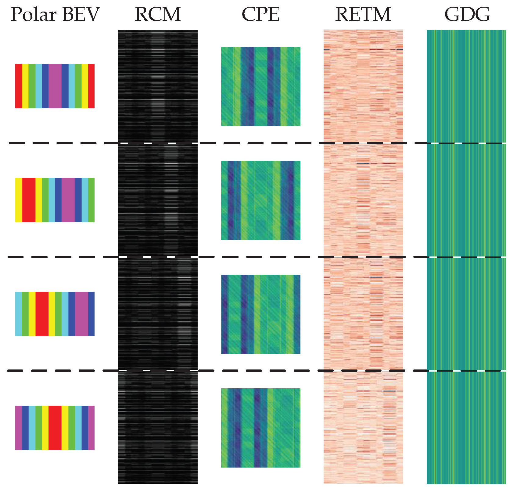
To intuitively illustrate the feature behavior of the proposed modules under controlled yaw rotations of the proposed network modules, we conduct a controlled visualization experiment. As shown in Figure 7, a color-striped image is employed as a simplified polar BEV input, with each row corresponding to rotation angles of 0°, 60°, 120°, and 180°, respectively. From left to right: the polar BEV input exhibits a cyclic column shift under rotation; the RCM compresses radial information while preserving the azimuthal structure; the CPE dynamically injects rotation-equivariant positional encoding; and the RETM further models long-range azimuthal dependencies. Finally, the output of the GDG remains visually consistent across all rotation angles, showing that the aggregated global descriptor remains visually consistent under controlled yaw rotations.

The above visualization provides a qualitative illustration that, under controlled yaw rotations, the proposed network modules can preserve the cyclic-shift structure of the polar BEV representation and produce consistent global descriptors after GDG aggregation. On this basis, to further quantitatively analyze the contribution of both the DHI input representation and the key network components to place recognition performance, we conduct ablation experiments on the LPRR dataset. For the DHI ablation, inspired by the pseudo-RGB input setting used in BEVPlace++ to adapt a single-channel BEV image to a ResNet backbone, each single-attribute polar BEV image is copied into three channels to keep the input size and network architecture unchanged. Specifically, the Density-only, Height-only, and Intensity-only variants use $[D,D,D]$, $[H,H,H]$, and $[I,I,I]$ as inputs, respectively, while the full model uses the proposed DHI input $[D,H,I]$. This design ensures that the comparison focuses on the contribution of different input attributes rather than changes in model capacity. For the module ablation, we remove or replace key components in the feature extractor to evaluate the roles of the RCM, CPE, CRPB, and RETM. All models involved in the ablation study adopt exactly the same training configuration as the full model and are evaluated under the same LPRR protocol. The quantitative comparison of the key metrics Recall@1 and Recall@25 is provided in

Table 5. Ablation study results of Recall@1 and Recall@25 on the key components.

Variant	Recall@1	Recall@25
Density-only	0.471	0.853
Height-only	0.425	0.767
Intensity-only	0.413	0.746
w/o RCM	0.543	0.924
w/o CPE	0.511	0.877
w/o CRPB	0.503	0.912
w/o RETM	0.550	0.901
Ours	0.599	0.970

Abbreviations: RCM, Radial Compression Module; CPE, Conditional Positional Encoding; CRPB, Circular Relative-Position Bias; RETM, rotation-equivariant Transformer module.

.

Validation of the DHI. To evaluate the effectiveness of the proposed DHI polar BEV representation, we compare the full DHI input with three three-channel replicated single-attribute variants. As shown in Table 5, the Density-only, Height-only, and Intensity-only variants achieve Recall@1 values of 0.471, 0.425, and 0.413, respectively, and Recall@25 values of 0.853, 0.767, and 0.746, respectively. In contrast, the full DHI representation improves Recall@1 to 0.599 and Recall@25 to 0.970. These results indicate that the three input attributes provide complementary information for place recognition: density captures the spatial distribution of LiDAR points, height encodes geometric structure, and intensity introduces reflectance cues. Their joint use therefore enhances the discriminability and robustness of the learned global descriptor.

Validation of the RCM. To verify the necessity of the proposed axis-wise separable convolution with circular padding, we replace the axis-wise separable convolutions in the RCM with standard convolutions, while keeping the remaining network architecture consistent with the full model. As shown in Table 5, the Recall@1 of this variant drops from 0.599 to 0.543, and the Recall@25 drops from 0.970 to 0.924. Although the absolute drops in Recall@1 appear modest, the consistent degradation across both metrics confirms that each module contributes distinct and complementary properties: the RCM preserves geometric equivariance, while the RETM enhances discriminative power through global contextualization.

Validation of the CPE. To assess the effectiveness of CPE, we construct a w/o CPE variant by removing the CPE module from the RETM and using no additional positional encoding, so that the feature sequence output by the RCM is directly fed into the multi-head self-attention layers. The remaining network architecture and training configuration are kept unchanged. As presented in Table 5, the w/o CPE variant yields a Recall@1 of 0.511 and a Recall@25 of 0.877, which are lower than the full model by 0.088 and 0.093, respectively. This performance degradation shows that CPE is beneficial for injecting local azimuthal positional information into the feature sequence. Without CPE, the Transformer has weaker capability to encode position-aware relationships among neighboring azimuthal tokens, resulting in reduced descriptor discriminability.

Validation of the CRPB. To verify the necessity of CRPB, we construct a w/o CRPB variant by replacing the proposed circular-relative-bias self-attention with standard multi-head self-attention, where the attention score is computed only from the query-key similarity without adding any Circular Relative-Position Bias. The other components are kept unchanged. As shown in Table 5, the w/o CRPB variant obtains a Recall@1 of 0.503 and a Recall@25 of 0.912, which are lower than the full model by 0.096 and 0.058, respectively. These results confirm that CRPB helps the attention mechanism explicitly model the circular relative distances among azimuthal tokens. Without CRPB, the Transformer lacks circular relative-position modeling, leading to weaker long-range azimuthal contextual reasoning and reduced place recognition performance.

Validation of the RETM. To evaluate the effectiveness of the proposed RETM in modeling long-range azimuthal dependencies, we remove the RETM and reshape the RCM output from $1\times N_{\theta }\times C$ to $N_{\theta }\times C$, which is then directly fed into NetVLAD. This variant aims to test the capability of place recognition using only local azimuthal features without global contextual interactions along the azimuthal dimension. As presented in Table 5, this variant yields a Recall@1 of 0.550 and a Recall@25 of 0.901. This indicates that without the global contextual interactions introduced by the RETM, the network struggles to establish long-range azimuthal correlations, resulting in a degradation in the discriminability of the global descriptor, thereby validating the critical role of the RETM.

5.4. Runtime

In addition to recognition accuracy, computational efficiency is also a critical metric for determining whether a LiDAR place recognition algorithm can be practically deployed on resource-constrained autonomous driving platforms. In this section, we compare the runtime efficiency of the proposed algorithm with that of HOTFormerLoc, BEVPlace++, OverlapTransformer, and Scan Context on the KITTI dataset sequence 00.

To ensure a fair comparison of the online inference efficiency of different methods, the global descriptors of the database are pre-extracted offline according to the default configuration of each method. During the testing phase, timing starts from reading the raw point cloud file from disk and ends when retrieval matching is completed. Query frames of the KITTI dataset sequence 00 are tested continuously, frame by frame, and the average processing time per frame is recorded. The runtime metrics, including per-frame latency and throughput measured in frames per second (FPS), are reported in

Table 6. Comparison of model complexity and runtime performance among different LiDAR place recognition methods.

Method	Params (M)	Size (MB)	FLOPs (G)	Latency (ms)	FPS
HOTFormerLoc	35.37	134.93	2.47	44.90	22.26
BEVPlace++	1.36	5.20	10.84	118.31	8.45
OverlapTransformer	48.14	183.65	3.26	18.28	54.70
Scan Context	N/A	N/A	N/A	103.39	9.67
Ours	8.22	31.35	2.10	25.44	39.30

Scan Context is a non-learning method without trainable parameters.

.

To further avoid ambiguity in the runtime analysis, we decompose the query-time latency of the proposed method into its main pipeline components, as reported in

Table 7. Comparison of component-wise runtime performance among different stages of the proposed method.

Component	Total (s)	Avg. (ms)
Polar BEV Generation	28.86	21.52
Radial Compression Module	2.59	1.93
Rotation-Equivariant Transformer Module	2.12	1.58
Global Descriptor Generator	0.49	0.37
Database Matching	0.06	0.05
Overall Total	34.12	25.44

. The component-wise timing is averaged over 1341 query frames of KITTI sequence 00.

As shown in Table 6, BEVPlace++ achieves the most compact model with only 1.36 M parameters and a size of 5.20 MB. This compactness, however, comes with relatively high computational overhead, as evidenced by its 10.84 GFLOPs, 118.31 ms per-frame latency, and 8.45 FPS. OverlapTransformer has the largest parameter count, with 48.14 M parameters and a model size of 183.65 MB, but achieves the fastest runtime, with a latency of 18.28 ms and 54.70 FPS. HOTFormerLoc occupies a middle ground in terms of model size and speed, achieving a latency of 44.90 ms and 22.26 FPS. Scan Context, although free of trainable parameters, requires 103.39 ms per frame due to its hand-crafted descriptor construction and matching procedure.

The proposed method achieves a favorable balance between model complexity and runtime efficiency. It has 8.22 M parameters, roughly one-sixth of OverlapTransformer, and a model size of 31.35 MB, making it more compact than OverlapTransformer and HOTFormerLoc. Its computational cost of 2.10 GFLOPs is also the lowest among the learning-based methods. Although its latency of 25.44 ms and frame rate of 39.30 FPS are slightly lower than those of OverlapTransformer, they are substantially better than BEVPlace++, HOTFormerLoc, and Scan Context.

The component-wise analysis in Table 7 further shows that the main computational cost of the proposed method lies in Polar BEV generation, which takes 21.52 ms per frame and accounts for most of the total latency. This relatively high cost is mainly caused by point-cloud loading/parsing and CPU-based polar grid binning in the current implementation rather than the neural network itself. In contrast, the neural descriptor extraction stages are lightweight: the Radial Compression Module, rotation-equivariant Transformer module, and Global Descriptor Generator require only 1.93 ms, 1.58 ms, and 0.37 ms, respectively. Database matching is also efficient, requiring only 0.05 ms per query. These results indicate that the proposed feature encoder and retrieval stage introduce limited computational overhead, while further optimization of the Polar BEV generation stage, such as more efficient point-cloud loading and GPU-based parallel grid construction, could further improve online efficiency. Since common vehicle-mounted LiDAR typically operate at 10 Hz or 20 Hz, the proposed method shows potential for real-time LiDAR place recognition on autonomous driving platforms.

6. Conclusions

This paper presents a robust and efficient LiDAR place recognition framework that achieves strong performance under large yaw rotations while maintaining computational efficiency. By projecting raw point clouds into polar BEV grids with density, height, and intensity channels, and designing a rotation-equivariant feature encoder consisting of a Radial Compression Module and a rotation-equivariant Transformer module, our method produces compact global descriptors that exhibit strong robustness to large yaw rotations via NetVLAD with end-to-end hard example mining triplet loss. Extensive experiments on KITTI, NCLT, and the proposed LPRR dataset demonstrate that our approach achieves competitive or superior performance across the evaluated datasets and metrics, achieving superior recall rates with only 8.22 M parameters and 25.44 ms per frame. Ablation studies confirm the necessity of the proposed modules, and the results on NCLT and LPRR suggest promising cross-dataset generalization within the evaluated settings without fine-tuning.

In future work, we plan to relax the ground-flatness assumption to handle non-planar off-road scenarios with significant pitch and roll disturbances. We will also further evaluate the proposed method on more diverse real-world datasets and deployment scenarios to validate its generalization capability under broader environmental conditions. In addition, we will investigate integrating multi-modal sensor fusion, such as camera and IMU, and developing online adaptation strategies for long-term operation without full retraining.

References

1. Yin, H.; Xu, X.; Lu, S.; Chen, X.; Xiong, R.; Shen, S.; Stachniss, C.; Wang, Y. A Survey on Global LiDAR Localization: Challenges, Advances and Open Problems. Int. J. Comput. Vis. 2024, 132, 3139–3171. [Google Scholar] [CrossRef]
2. Geiger, A.; Lenz, P.; Urtasun, R. Are we ready for autonomous driving? The KITTI vision benchmark suite. In Proceedings of the 2012 IEEE Conference on Computer Vision and Pattern Recognition, Providence, RI, USA, 16–21 June 2012. [Google Scholar] [CrossRef]
3. Kim, G.; Kim, A. Scan Context: Egocentric Spatial Descriptor for Place Recognition Within 3D Point Cloud Map. In Proceedings of the 2018 IEEE/RSJ International Conference on Intelligent Robots and Systems (IROS), Madrid, Spain, 1–5 October 2018. [Google Scholar] [CrossRef]
4. Ma, J.; Zhang, J.; Xu, J.; Ai, R.; Gu, W.; Chen, X. OverlapTransformer: An efficient and yaw-angle-invariant transformer network for LiDAR-based place recognition. IEEE Robot. Autom. Lett. 2022, 7, 6958–6965. [Google Scholar] [CrossRef]
5. Carlevaris-Bianco, N.; Ushani, A.K.; Eustice, R.M. University of Michigan North Campus Long-Term Vision and Lidar Dataset. Int. J. Robot. Res. 2016, 35, 1023–1035. [Google Scholar] [CrossRef]
6. Uy, M.A.; Lee, G.H. PointNetVLAD: Deep point cloud based retrieval for large-scale place recognition. In Proceedings of the 2018 IEEE/CVF Conference on Computer Vision and Pattern Recognition, Salt Lake City, UT, USA, 18–23 June 2018. [Google Scholar] [CrossRef]
7. Liu, Z.; Zhou, S.; Suo, C.; Yin, P.; Chen, W.; Wang, H.; Li, H.; Liu, Y. LPD-Net: 3D point cloud learning for large-scale place recognition and environment analysis. In Proceedings of the 2019 IEEE/CVF International Conference on Computer Vision (ICCV), Seoul, Republic of Korea, 27 October–2 November 2019. [Google Scholar] [CrossRef]
8. Griffiths, E.; Haghighat, M.; Denman, S.; Fookes, C.; Ramezani, M. HOTFormerLoc: Hierarchical Octree Transformer for Versatile Lidar Place Recognition Across Ground and Aerial Views. In Proceedings of the 2025 IEEE/CVF Conference on Computer Vision and Pattern Recognition (CVPR), Nashville, TN, USA, 10–17 June 2025. [Google Scholar] [CrossRef]
9. Yin, P.; Jiao, J.; Zhao, S.; Xu, L.; Huang, G.; Choset, H.; Scherer, S.; Han, J. General place recognition survey: Toward real-world autonomy. IEEE Trans. Robot. 2025, 41, 3019–3038. [Google Scholar] [CrossRef]
10. Luo, L.; Cao, S.; Han, B.; Shen, H.; Li, J. BVMatch: Lidar-Based Place Recognition Using Bird’s-Eye View Images. IEEE Robot. Autom. Lett. 2021, 6, 6076–6083. [Google Scholar] [CrossRef]
11. Luo, L.; Zheng, S.; Li, Y.; Fan, Y.; Yu, B.; Cao, S.; Li, J.; Shen, H. BEVPlace: Learning LiDAR-based Place Recognition using Bird’s Eye View Images. In Proceedings of the 2023 IEEE/CVF International Conference on Computer Vision (ICCV), Paris, France, 1–6 October 2023. [Google Scholar] [CrossRef]
12. Arandjelović, R.; Gronat, P.; Torii, A.; Pajdla, T.; Sivic, J. NetVLAD: CNN architecture for weakly supervised place recognition. IEEE Trans. Pattern Anal. Mach. Intell. 2018, 40, 1437–1451. [Google Scholar] [CrossRef] [PubMed]
13. Luo, L.; Cao, S.; Li, X.; Xu, J.; Ai, R.; Yu, Z.; Chen, X. BEVPlace++: Fast, robust, and lightweight LiDAR global localization for autonomous ground vehicles. IEEE Trans. Robot. 2025, 41, 4479–4498. [Google Scholar] [CrossRef]
14. He, K.; Zhang, X.; Ren, S.; Sun, J. Deep residual learning for image recognition. In Proceedings of the 2016 IEEE Conference on Computer Vision and Pattern Recognition (CVPR), Las Vegas, NV, USA, 27–30 June 2016. [Google Scholar] [CrossRef]
15. Jiang, W.; Xue, H.; Si, S.; Xiao, L.; Zhao, D.; Zhu, Q.; Nie, Y.; Dai, B. R2SCAT-LPR: Rotation-robust network with self- and cross-attention transformers for LiDAR-based place recognition. Remote Sens. 2025, 17, 1057. [Google Scholar] [CrossRef]
16. Shen, Y.; Tuna, T.; Hutter, M.; Cadena, C.; Zheng, N. ForestLPR: LiDAR Place Recognition in Forests Attentioning Multiple BEV Density Images. In Proceedings of the 2025 IEEE/CVF Conference on Computer Vision and Pattern Recognition (CVPR), Nashville, TN, USA, 10–17 June 2025. [Google Scholar] [CrossRef]
17. Kim, G.; Choi, S.; Kim, A. Scan Context++: Structural Place Recognition Robust to Rotation and Lateral Variations in Urban Environments. IEEE Trans. Robot. 2022, 38, 1856–1874. [Google Scholar] [CrossRef]
18. Chen, X.; Läbe, T.; Milioto, A.; Röhling, T.; Vysotska, O.; Haag, A.; Behley, J.; Stachniss, C. OverlapNet: Loop closing for LiDAR-based SLAM. In Proceedings of the Robotics: Science and Systems, Corvallis, OR, USA, 12–16 July 2020. [Google Scholar] [CrossRef]
19. Ma, J.; Chen, X.; Xu, J.; Xiong, G. SeqOT: A spatial-temporal transformer network for place recognition using sequential LiDAR data. IEEE Trans. Ind. Electron. 2023, 70, 8225–8234. [Google Scholar] [CrossRef]
20. Ma, J.; Xiong, G.; Xu, J.; Chen, X. CVTNet: A Cross-View Transformer Network for LiDAR-Based Place Recognition in Autonomous Driving Environments. IEEE Trans. Ind. Inform. 2024, 20, 4039–4048. [Google Scholar] [CrossRef]
21. Luo, J.; Cheng, J.; Xiang, Q.; Wu, J.; Fan, R.; Chen, X.; Tang, X. OverlapMamba: A shift state space model for LiDAR-based place recognition. IEEE Robot. Autom. Lett. 2025, 10, 8380–8387. [Google Scholar] [CrossRef]
22. Vaswani, A.; Shazeer, N.; Parmar, N.; Uszkoreit, J.; Jones, L.; Gomez, A.N.; Kaiser, Ł.; Polosukhin, I. Attention is all you need. In Proceedings of the 31st International Conference on Neural Information Processing Systems, Long Beach, CA, USA, 4–9 December 2017. [Google Scholar]
23. Chu, X.; Tian, Z.; Zhang, B.; Wang, X.; Shen, C. Conditional Positional Encodings for Vision Transformers. In Proceedings of the Eleventh International Conference on Learning Representations (ICLR 2023), Kigali, Rwanda, 1–5 May 2023. [Google Scholar]
24. Dosovitskiy, A.; Ros, G.; Codevilla, F.; Lopez, A.; Koltun, V. CARLA: An Open Urban Driving Simulator. In Proceedings of the 1st Annual Conference on Robot Learning (CoRL 2017), Mountain View, CA, USA, 13–15 November 2017. [Google Scholar]
25. Malkov, Y.A.; Yashunin, D.A. Efficient and Robust Approximate Nearest Neighbor Search Using Hierarchical Navigable Small World Graphs. IEEE Trans. Pattern Anal. Mach. Intell. 2020, 42, 824–836. [Google Scholar] [CrossRef] [PubMed]
Figure 1. Multi-view revisits at an intersection in KITTI Sequence 08. (Left): trajectory overlaid on a satellite map, where blue denotes trajectory segments without revisits, red denotes revisited trajectory segments, and the yellow rectangle marks the intersection. (Middle top): zoomed-in aerial view corresponding to the yellow rectangle, with red circles 1–4 marking observation positions. (Middle bottom): LiDAR BEV representation at Frame 1505, with the vehicle at the center of the intersection. (Right): onboard camera images at Frames 687, 749, 1478, and 1510.
Applsci 16 06155 g001
Figure 2. Pipeline overview of our proposed approach. The proposed place recognition framework comprises three consecutive stages: (first) Pre-processing, where raw point clouds are clipped and gridded to generate three-channel polar BEV images encoding intensity, height, and density information; (second) Place Modeling, which first employs a Radial Compression Module (RCM) to derive compact azimuthal feature sequences. Subsequently, a rotation-equivariant Transformer module (RETM) equipped with Conditional Positional Encoding (CPE) processes these sequences to dynamically inject rotation-equivariant positional information and model long-range contextual dependencies. The encoded features are then aggregated into a global representation via NetVLAD, projected to a low-dimensional vector by a fully connected (FC) layer, and L2-normalized to yield the final global descriptor; and (third) Place Matching, where the query global descriptor is retrieved against a pre-built descriptor map through approximate nearest neighbor search to obtain the loop candidates.
Applsci 16 06155 g002
Figure 3. Trajectory visualization overlaid on satellite maps. (Left): trajectory of the KITTI 00 sequence; (middle): trajectory of the NCLT 2012-01-08 sequence; (right): trajectory of the self-constructed LiDAR Place Recognition Revisit (LPRR) dataset built upon the CARLA simulation platform.
Applsci 16 06155 g003
Figure 4. Example of sensor data at an intersection scene in the self-constructed LiDAR Place Recognition Revisit (LPRR) dataset: (a) global trajectory of the data collection route, where the red and green curves indicate two traversal directions and the yellow rectangle marks the selected intersection area; (b) enlarged local view of the intersection, where the red circles indicate representative data acquisition positions; (c) synchronized sensor observations at eight acquisition positions, where the upper images show LiDAR point clouds in BEV form and the lower images show the corresponding forward-view camera images. Positions 5/6 and 7/8 correspond to different vehicle headings at spatially close locations, illustrating appearance variations caused by viewpoint changes.
Applsci 16 06155 g004
Figure 5. Recall@K curves on three benchmark datasets: (a) KITTI; (b) NCLT; (c) LiDAR Place Recognition Revisit (LPRR).
Applsci 16 06155 g005
Figure 6. Top-1 threshold-based precision-recall curves on three benchmark datasets: (a) KITTI; (b) NCLT; (c) LiDAR Place Recognition Revisit (LPRR).
Applsci 16 06155 g006
Figure 7. Demonstration of the rotation equivariance and invariance of the network modules. A color-striped image is employed as a simplified example input for the polar BEV representation. From left to right: polar BEV input, Radial Compression Module (RCM) output features, Conditional Positional Encoding (CPE), rotation-equivariant Transformer module (RETM) output features, and Global Descriptor Generator (GDG) output. Each row corresponds to the input image rotated by 0 , 60 , 120 , and 180 , respectively.
Applsci 16 06155 g007