Multi-Objective Optimization in Injection Molding Simulation: A Preference-Driven Approach with an Adaptive Experimental Design to Investigate the Optimal Solution Region

Abstract

This contribution presents a simulation-based approach for optimizing injection molding processes using digital twins. It combines surrogate modeling via response surface methodology (RSM) with the evolutionary algorithm NSGA-II to efficiently capture complex relationships between process parameters and objectives. A key element is the adaptive enhancement of the training dataset within the decision-relevant region of interest (ADEROI) by a modified greedy max–min algorithm. This strategy closes data gaps, improves model accuracy in the potentially optimal region, and directs additional simulations to informative areas. Leave-one-out (LOO) and hold-out (HO) cross-validations show strong root mean square error (RMSE) and $R^2$ values for deformation, shrinkage, cycle time, and mass. NSGA-II converges after 403 generations and results in 191 Pareto-optimal solutions, which are consolidated into preference-consistent operating points. These points make trade-offs between analyzed objectives’ deformation, shrinkage, and cycle time explicit for process pre-design. Preferred solutions are identified through weighted sums of normalized objectives and inversely mapped process parameters. Their agreement with the physics-based digital twin at the hundredths level supports the plausibility of the selected operating points within the investigated simulation-based workflow. A retrospective benchmark against a scaled single-stage LHS baseline shows that ADEROI achieves ROI-equivalent point density with fewer simulation runs for the investigated case, reducing the estimated runtime by $39.1\%$ and resulting in a $1.64\times$ speed-up. The quantitative validation is limited to one thin-walled PP keyholder component; further geometries, mold layouts, and polymer materials are required to empirically assess generalizability.

1. Introduction

Injection molding is a key process in polymer manufacturing, enabling the efficient production of high-quality components with complex geometries. Advances in simulation software have improved the prediction of process parameters, but detailed simulation models remain computationally expensive. This is mainly due to the need to resolve multiphysical phenomena such as heat transfer, solidification, non-Newtonian fluid dynamics, and complex material behavior [1]. To address these challenges, surrogate modeling techniques have become an established approach for reducing computational cost while maintaining sufficient model accuracy [2,3].

Process parameter optimization is traditionally performed using experimental approaches such as design of experiments (DoE) in combination with RSM [4]. However, simulation-based optimization offers considerable flexibility and efficiency, particularly when combined with surrogate models such as RSM or Kriging [5]. These models can substantially reduce the computational effort required for complex simulation models [6,7]. Alternative surrogate modeling techniques, including neural networks and random forests, have also been investigated [8,9,10]. However, these methods often require larger training data sets and are less straightforward to interpret. In addition, they do not always provide an optimal balance between accuracy and computational efficiency compared with classical surrogate models [8,9].

Several studies have demonstrated the potential of surrogate-based optimization in injection molding. For example, ref. [11] combined RSM with a multi-objective evolutionary algorithm (NSGA-II) for automotive fender injection molding and successfully balanced energy efficiency and product quality. Similarly, ref. [12] integrated an artificial neural network (ANN) surrogate with NSGA-II to simultaneously optimize dimensional accuracy, cycle time, and energy consumption. In addition, ref. [13] applied Latin hypercube sampling to train an ANN surrogate for microcellular injection molding, achieving improvements in energy usage, weight, and warpage. Further studies by [14,15] demonstrated the effectiveness of RSM in surrogate modeling and multi-objective process optimization. These authors used RSM together with complementary techniques such as the Taguchi method and genetic algorithms to optimize injection molding parameters. Their results showed that process parameters such as melt temperature and injection pressure can significantly reduce shrinkage, warpage, and other quality-related defects.

In summary, the integration of surrogate models into simulation-based optimization frameworks represents an important advancement in injection molding. It can reduce computational cost while improving the robustness and accuracy of process optimization, thereby supporting more efficient and effective manufacturing processes.

The combination of surrogate models and optimization algorithms offers considerable potential for injection molding simulations by reducing both computational time and resource consumption. In particular, integrating RSM with optimization algorithms such as NSGA-II has proven effective for improving the efficiency of process optimization. NSGA-II is widely regarded as a benchmark algorithm for multi-objective optimization and is extensively used in manufacturing and other real-world applications. Compared with alternative evolutionary multi-objective optimization algorithms, previous studies have reported high solution quality, computational efficiency, and robust population diversity [16,17,18,19,20], as well as strong practical applicability [17,21,22]. In injection molding, NSGA-II has been shown to be an effective method for multi-objective process optimization [12,14,23,24,25,26,27,28]. Within the proposed framework, NSGA-II is considered a suitable candidate optimizer because it operates without derivatives, requires limited parameter tuning, and uses elitism and crowding distance to maintain diverse Pareto front approximations. Its final selection is further supported by the comparative benchmark presented in Section 6.

This study presents a systematic implementation and analysis of surrogate-based multi-objective optimization for injection molding simulations using digital twin technology (cf. Figure 1). As shown in Figure 1, digital twin level 1 represents the generation of a physical injection molding simulation model based on Cadmould 3D-F simulations, with training data points obtained from Latin hypercube sampling (LHS). Digital twin level 2 describes the generation of RSM-based surrogate models that represent digital twin level 1. In this study, digital twins are understood as virtual representations of physical systems [29,30,31,32].

The aim of this study is to introduce a framework for the systematic expansion of training data, the optimization of injection molding process parameters, and the preference-based evaluation of Pareto-optimal solutions. The training data are adaptively enhanced in the region of interest (ADEROI) using the surrogate model. This approach approximates the relevant optimization region and enriches it with new training data through a modified greedy max-min strategy. In addition, a preference-based solution identification method is introduced to select Pareto-optimal solutions according to the relative importance of the objectives.

The proposed framework is investigated for a preference-driven multi-objective optimization problem in injection molding involving six process parameters and three objectives: deformation, shrinkage, and cycle time, with mass treated as a constraint. The RSM-based surrogate models are initialized using a Latin hypercube design with 100 sampling points. Subsequently, 100 ROI-focused samples are added through ADEROI and the modified greedy max-min strategy, resulting in a $1.64\times$ speed-up compared to a larger LHS. The NSGA-II optimization is performed over 403 generations and results in 191 Pareto-optimal solutions. Practically relevant operating points are then identified using weighting methodologies. Although the study focuses on a single geometry and material, generalization aspects, limitations, and implementation details are discussed in the associated methods.

2. Numerical Simulation of Injection Molding Process

An accurate representation of the polymer melt flow into thin mold cavities, typical for thin-walled polymer parts, can be achieved using a two-dimensional incompressible flow model based on the mid-surface approximation, as implemented in the commercial simulation software Cadmould 3D-F. In this modeling approach, the Hele–Shaw approximation, derived from the Navier–Stokes equations, is applied [33]. The respective conservation laws for mass, momentum, and energy are employed to accurately describe the filling and holding pressure phases during injection molding. During the cooling phase, Cadmould 3D-F employs a comprehensive approach to compute both heat transfer and stress evolution. The heat transfer calculations are performed individually for each specific region of the cavity, allowing for a detailed and accurate representation of the thermal behavior within the system. In order to predict shrinkage and warpage of the molded part, it is necessary to determine the residual stresses by means of a viscous-thermoelastic approach. Such an approach is implemented in the software Cadmould 3D-F [34]. For further details on the simulation model, the authors refer to their former research [5,34,35,36,37,38]. In the further course of investigations, the numerical simulation model serves as the physics-based numerical reference model for all surrogate models. In an industrial context, this model can also be replaced by the real process in an injection molding machine.

3. Surrogate Models

Surrogate models are an essential part of computational modeling and simulation for approximating complex systems that are otherwise computationally expensive. These models have been developed to reduce the computational cost and simplify the analysis, optimization, and uncertainty quantification of complex systems by approximating the behavior of the original system [39]. This section describes the surrogate modeling approach based on RSM.

RSM is a statistical technique designed to explore the relationship between multiple independent variables and one or more dependent responses [40]. It is particularly useful in process optimization because it approximates how changes in input variables influence system behavior. In practice, RSM employs regression analysis to fit a polynomial model to experimental data [41]. The following equation is a general formulation of the flexible polynomial RSM [42]:

$$\begin{array}{c}\hfill y\left(x\right)={\beta }_0+{\displaystyle \sum _{m=1}^d}{\displaystyle \sum _{i=1}^k}{\beta }_{i,m}{x}_i^m+{\displaystyle \sum _{m=1}^d}\sum _{i<j}{\beta }_{ij,m}{x}_i^m{x}_j^m+{ϵ}_i\end{array}$$

(1)

In this context, the function $y:{\mathbb{R}}^k\mapsto \mathbb{R}$ represents the predicted response of the model based on the input vector $x\in {\mathbb{R}}^k$, where k is the number of input factors. The intercept term ${\beta }_0\in \mathbb{R}$ represents the expected response when all inputs are zero. The coefficient ${\beta }_{i,m}\in \mathbb{R}$ quantifies the individual effect of each input $x_i$ at the m-th order [43]. The flexible polynomial RSM model can include linear terms ${\beta }_{i,1}{x}_i$, quadratic terms ${\beta }_{i,2}{x}_i^2$, and higher-order terms ${\beta }_{i,m}{x}_i^m$ up to a maximum order d. The interaction terms ${\beta }_{ij,m}{x}_i^m{x}_j^m$ represent the combined effects of the two input variables $x_i$ and $x_j$ at the m-th order on the objective variable. A non-zero value for the interaction term ${\beta }_{ij,m}\in \mathbb{R}$ indicates that the effect of one variable on the response is dependent on the level of the other variable and highlights interaction effects within the system [41]. The residual error term ${ϵ}_i\in \mathbb{R}$ is the difference between the observed data and the model prediction. The residual error term describes the impact of random fluctuations, measurement inaccuracies, and other sources of variability in the data. The residual error term is described by the following equation:

$$\begin{array}{c}\hfill {ϵ}_i=y_{\mathrm{obs},i}-{\widehat{y}}_i\end{array}$$

(2)

In this equation, $y_{\mathrm{obs},i}\in \mathbb{R}$ represents the actual observed values, ${\widehat{y}}_i\in \mathbb{R}$ denotes the values predicted by the RSM model for a given observation, and i is the number of observations [42].

The RSM model is developed to determine the coefficients ${\beta }_0$, ${\beta }_{i,m}$, and ${\beta }_{ij,m}$ by fitting the model to the experimental data using a least squares approach. This involves the reduction of the sum of the squared deviations between the actual responses and the predictions of the model [41]. Once these parameters have been established, the model can predict results for new input scenarios and clarify the influence of different inputs on the response.

4. Multi-Objective Optimization with NSGA-II and Comparative Pareto Front Quality Assessment

Evolutionary algorithms have been proven to be a flexible and powerful method for solving complex, multi-dimensional, and nonlinear multi-objective optimization problems. The algorithms do not depend on derivatives or exact gradient information but use population-based search methods. These methods aim to approximate the Pareto front while maintaining solution diversity and they do not rely on derivatives or exact gradients. In this context, it is important to note that the decision variables are expressed as the vector $x\in {\mathbb{R}}^n$, where $x_i$ are components in ${\mathbb{R}}^n$. The constrained multi-objective minimization problem for M scalar-valued objective functions $f_{•}:{\mathbb{R}}^n\to \mathbb{R}$ can be defined as follows:

$$\begin{array}{c}\hfill \begin{array}{cc}\hfill & \underset{x\in \mathcal{X}}{\min }f\left(x\right)={\left(f_1\left(x\right),\dots ,f_M\left(x\right)\right)}^{\top }\hfill \\ \hfill & \mathcal{X}=\{x\in {\mathbb{R}}^n\mid {\ell }_i\le x_i\le u_i,g_j\left(x\right)\le 0,h_p\left(x\right)=0\}\hfill \end{array}\end{array}$$

(3)

In this context, ${\ell }_i\le x_i\le u_i$ for $i=1,\dots ,n$ denote the component-wise lower/upper bounds; $g:{\mathbb{R}}^n\to {\mathbb{R}}^{m_{\mathrm{ineq}}}$ collects the inequality constraints with $g_j\left(x\right)\le 0$ understood element-wise; and $h:{\mathbb{R}}^n\to {\mathbb{R}}^{m_{\mathrm{eq}}}$ collects the equality constraints (i.e., $h_p\left(x\right)=0$). A feasible point $x^{*}\in \mathcal{X}$ is Pareto-optimal if no $x\in \mathcal{X}$ exists with $x\prec x^{*}$, where the Pareto set is ${\mathcal{P}}^{\star }$ and the global Pareto front is $f\left({\mathcal{P}}^{\star }\right)$.

The aim of evolutionary algorithms is to generate a set of solutions $P\subset {\mathbb{R}}^n$ that represent a good approximation of the Pareto front. Evolutionary algorithms are based on the principles of natural selection as well as genetic variation and were developed in their original form for modeling biological evolution [44].

The fundamental elements of these algorithms include population, generation, selection, crowding distance, crossover, mutation, and fitness evaluation. The population, denoted by $P_t=x_1^t,x_2^t,\dots ,x_N^t$, represents the set of individuals (solutions) N that are analyzed simultaneously in each generation (iteration step) t. Each individual $x\in P_t$ is evaluated using the objective function values $f\left(x\right)={(f_1\left(x\right),f_2\left(x\right),\dots ,f_M\left(x\right))}^T$. The selection describes the process of choosing individuals based on their fitness. Higher fitness values are associated with a greater probability of reproduction. In the context of multi-objective optimization, fitness is quantified according to Pareto dominance and additional diversity measures [45,46]. The dominance relation $x\prec y$ for two individuals $x,y\in P_t$ is defined as follows [45]:

$$\begin{array}{c}\hfill x\prec y\iff f_i\left(x\right)\le f_i\left(y\right)\forall i\mathrm{and}\exists j\mathrm{with}{f}_j\left(x\right)<f_j\left(y\right)\end{array}$$

(4)

The population is divided into non-dominated fronts $F_1,F_2,\dots ,F_k$ according to the following relation. In this context, $F_1$ denotes the set of all non-dominated individuals, while $F_2$ represents the non-dominated individuals of the remaining set [47].

The crowding distance, denoted by $d\left(x\right)$, quantifies the density of solutions around an individual x in a given Pareto front $F_k$ and promotes the preservation of diversity in the population. For each objective $f_i$, the front $F_k$ is first sorted in ascending order to produce a sequence $x_1^i,x_2^i,\dots ,x_{|F_k|}^i$. The distance to its nearest neighbors along the objective $f_i$ is then computed for each individual $x=x_j^i$. This method corresponds to an approximation of the edge of a rectangular region around the individual without containing other solutions [48] (cf. Figure 2). The total crowding distance $d\left(x\right)$ is then determined by summing the normalized distances over all objectives [48]. The extreme points of a Pareto front are assigned an infinite crowding distance to prevent them from disappearing from the population. The crowding-distance-based selection guarantees the consideration of these points during the subsequent generation, in addition to promoting the expansion of the Pareto front. The application of this method thus ensures a preference for individuals in regions with a low population density and a high crowding distance, which results in an optimal coverage of the Pareto front.

The following equation gives an approximation of the crowding distance for an individual $x=x_j^i$ [49]:

$$\begin{array}{c}\hfill d\left(x\right)={\displaystyle \sum _{i=1}^M}{\displaystyle \frac{f_i\left(x_{(j+1)}^i\right)-f_i\left(x_{(j-1)}^i\right)}{f_i^{\max }-f_i^{\min }}}\end{array}$$

(5)

In this context, $f_i^{\max }$ and $f_i^{\min }$ represent the maximum and minimum values of the objectives in the front. The individuals at the edges have an infinite distance to guarantee their selection [47]. The SBX-Crossover, a genetic operator, allows the combination of two parents $x^1,x^2\in {\mathbb{R}}^n$ with high fitness values to produce a new child y. The following equation applies to each element $k\in 1,\dots ,n$ [50]:

$$\begin{array}{c}\hfill y_k={\displaystyle \frac{1}{2}}\left[(1+{\beta }_q)x_k^1+(1-{\beta }_q)x_k^2\right]\end{array}$$

(6)

This contains the random parameter ${\beta }_q$, which is determined as a function of a random variable $u\in [0,1]$ and the distribution index ${\eta }_c$ [45,50].

$${\beta }_q=\left\{\begin{array}{cc}{\left(2u\right)}^{{\displaystyle \frac{1}{{\eta }_c+1}}}\hfill & , \mathrm{if}u\le 0.5\hfill \\ {\left({\displaystyle \frac{1}{2(1-u)}}\right)}^{{\displaystyle \frac{1}{{\eta }_c+1}}}\hfill & , \mathrm{if}u>0.5\hfill \end{array}\right\}$$

(7)

Mutation is defined as a genetic operator that is a random variation in individuals. The modified gene $x_k^{\prime }$ is determined for each element k according to the following equation:

$$\begin{array}{c}\hfill x_k^{\prime }=x_k+{\Delta }_k\left(x_k^{\max }-x_k^{\min }\right)\end{array}$$

(8)

Here, the random variable ${\Delta }_k$ is generated within the interval $[0,1]$, taking into account the allowed restrictions of the k-th gene by $x_k^{\max }$ and $x_k^{\min }$ [51]. These operators prevent the population from being restricted to local optima and encourage the exploration of new regions in the Pareto space [44,51]. The evaluation of the suitability of individual solutions is based on criteria that take into account compliance with Pareto dominance. This evaluation enables the specific selection of individuals that represent an acceptable compromise between competitive objectives [45]. The iterative application of these elements results in a population that is optimally close to the Pareto front. This iterative approach allows multiple optimal solutions to be approached simultaneously, taking into account different conflicting objectives.

The NSGA-II integrates the essential elements of evolutionary algorithms to form an iterative optimization procedure [47]. Within each generation t, a combined set $R_t=P_t\cup Q_t$ is obtained, where $Q_t$ represents the population of offspring generated by the genetic operators. Subsequently, a division of $R_t$ into non-dominated fronts $F_1,F_2,\dots ,F_k$ is carried out. The subsequent generation $P_{t+1}$ is determined by the selection of the best individuals N, according to the rank $r\left(x\right)$ and the crowding distance $d\left(x\right)$. This process can be described as follows, employing the comparison operator ${\prec }_{\mathrm{NSGA-II}}$.

$$\begin{array}{c}\hfill x{\prec }_{\mathrm{NSGA-II}}y\iff (r\left(x\right)<r\left(y\right))\mathrm{or}(r\left(x\right)=r\left(y\right)\mathrm{and}d\left(x\right)>d\left(y\right))\end{array}$$

(9)

The approach of the NSGA-II is shown in Figure 3 and can be divided into a three-phase process. These are the sorting of non-dominated solutions, the sorting of crowding distance, and genetic operations. This process guarantees both the convergence to the Pareto front and the diversity of the solutions. The division into non-dominated fronts, combined with the selection of the best individuals based on rank and crowding distance, ensures that the optimization process converges to the Pareto-optimal solutions with the maximum diversity of solutions.

For the comparative Pareto front quality assessment, two additional classical multi-objective optimizers are considered in addition to NSGA-II. These are the multi-objective particle swarm optimization (MOPSO) and the multi-objective evolutionary algorithm based on decomposition (MOEA/D). The three algorithms represent complementary search principles. NSGA-II is based on Pareto dominance and crowding distance, MOPSO follows a swarm-based search mechanism with an external archive of non-dominated solutions, and MOEA/D decomposes the multi-objective optimization problem into a set of scalar subproblems. This selection enables a compact comparison of dominance-based, swarm-based, and decomposition-based Pareto search strategies under identical surrogate- model conditions.

MOPSO extends the particle swarm optimization principle to multi-objective optimization problems [52]. Each individual is represented by a particle with position $x_i^t\in {\mathbb{R}}^n$ and velocity $v_i^t\in {\mathbb{R}}^n$ in generation t. The movement of the particle is influenced by its personal best position $p_i^t$ and by a leader $g_i^t$ selected from an external archive of non-dominated solutions. The velocity and position update can be expressed as follows:

$$\begin{array}{c}\hfill v_i^{t+1}=\chi v_i^t+c_1{\rho }_1\left(p_i^t-x_i^t\right)+c_2{\rho }_2\left(g_i^t-x_i^t\right)\end{array}$$

(10)

$$\begin{array}{c}\hfill x_i^{t+1}=x_i^t+v_i^{t+1}\end{array}$$

(11)

In this context, $\chi$ denotes the inertia factor, $c_1$ and $c_2$ are acceleration coefficients, and ${\rho }_1,{\rho }_2\in [0,1]$ are random numbers. The external archive stores the current set of non-dominated solutions and provides elitism during the optimization process. In addition, the selection of archive leaders can be used to promote diversity by preferring sparsely populated regions of the approximated Pareto front. MOPSO therefore provides a swarm-based reference method for comparison with the dominance-based NSGA-II.

MOEA/D follows a different strategy by decomposing the multi-objective optimization problem into several scalar optimization subproblems [53]. Each subproblem is associated with a weight vector ${\omega }^j={({\omega }_1^j,\dots ,{\omega }_M^j)}^{\top }$, where $j=1,\dots ,N$. The distribution of these weight vectors supports the coverage of the objective space. A common formulation is based on the Tchebycheff scalarization, which can be written as follows:

$$\begin{array}{c}\hfill g^{\mathrm{te}}\left(x\mid {\omega }^j,z^{\star }\right)=\underset{1\le i\le M}{max}\left\{{\omega }_i^j\left|f_i\left(x\right)-z_i^{\star }\right|\right\}\end{array}$$

(12)

Here, $z^{\star }={(z_1^{\star },\dots ,z_M^{\star })}^{\top }$ denotes the ideal point in the objective space. Each scalar subproblem is optimized in cooperation with neighboring subproblems, which are defined based on the distance between the corresponding weight vectors. This neighborhood structure enables local information exchange and supports both convergence and diversity. MOEA/D therefore provides a decomposition-based reference method for the comparative assessment of Pareto front quality.

To quantify the quality of the approximated Pareto fronts, the hypervolume indicator (HV) and the inverted generational distance (IGD) are used. Let $\mathcal{A}=a_1,\dots ,a_q$ denote an approximated Pareto front in the objective space and let $r^{\mathrm{HV}}={(r_1^{\mathrm{HV}},\dots ,r_M^{\mathrm{HV}})}^{\top }$ be a reference point that is dominated by all relevant non-dominated solutions for a minimization problem. The hypervolume is defined as the M-dimensional measure of the objective-space region dominated by $\mathcal{A}$ and bounded by $r^{\mathrm{HV}}$.

$$\begin{array}{c}\hfill HV(\mathcal{A},r^{\mathrm{HV}})={\lambda }_M\left(\bigcup _{a\in \mathcal{A}}[a_1,r_1^{\mathrm{HV}}]\times [a_2,r_2^{\mathrm{HV}}]\times \cdots \times [a_M,r_M^{\mathrm{HV}}]\right)\end{array}$$

(13)

In this equation, ${\lambda }_M$ denotes the M-dimensional Lebesgue measure. For a minimization problem, a larger hypervolume indicates a better Pareto front, since a larger region of the objective space is dominated. The IGD evaluates the average distance between a reference Pareto front ${\mathcal{P}}_{\mathrm{ref}}$ and the approximated Pareto front $\mathcal{A}$. It is defined as follows:

$$\begin{array}{c}\hfill IGD({\mathcal{P}}_{\mathrm{ref}},\mathcal{A})={\displaystyle \frac{1}{|{\mathcal{P}}_{\mathrm{ref}}|}}\sum _{p\in {\mathcal{P}}_{\mathrm{ref}}}\underset{a\in \mathcal{A}}{min}∥p-a∥\end{array}$$

(14)

A smaller IGD indicates that the approximated Pareto front is closer to the reference front and provides better coverage of it. In this contribution, HV and IGD are calculated in the normalized objective space. A common hypervolume reference point $r^{\mathrm{HV}}$ is used for all algorithms, and the IGD reference front ${\mathcal{P}}_{\mathrm{ref}}$ is constructed from the non-dominated union of the final Pareto fronts obtained by NSGA-II, MOPSO, and MOEA/D. This ensures that all algorithms are evaluated under identical Pareto front quality criteria.

5. Numerical Modeling

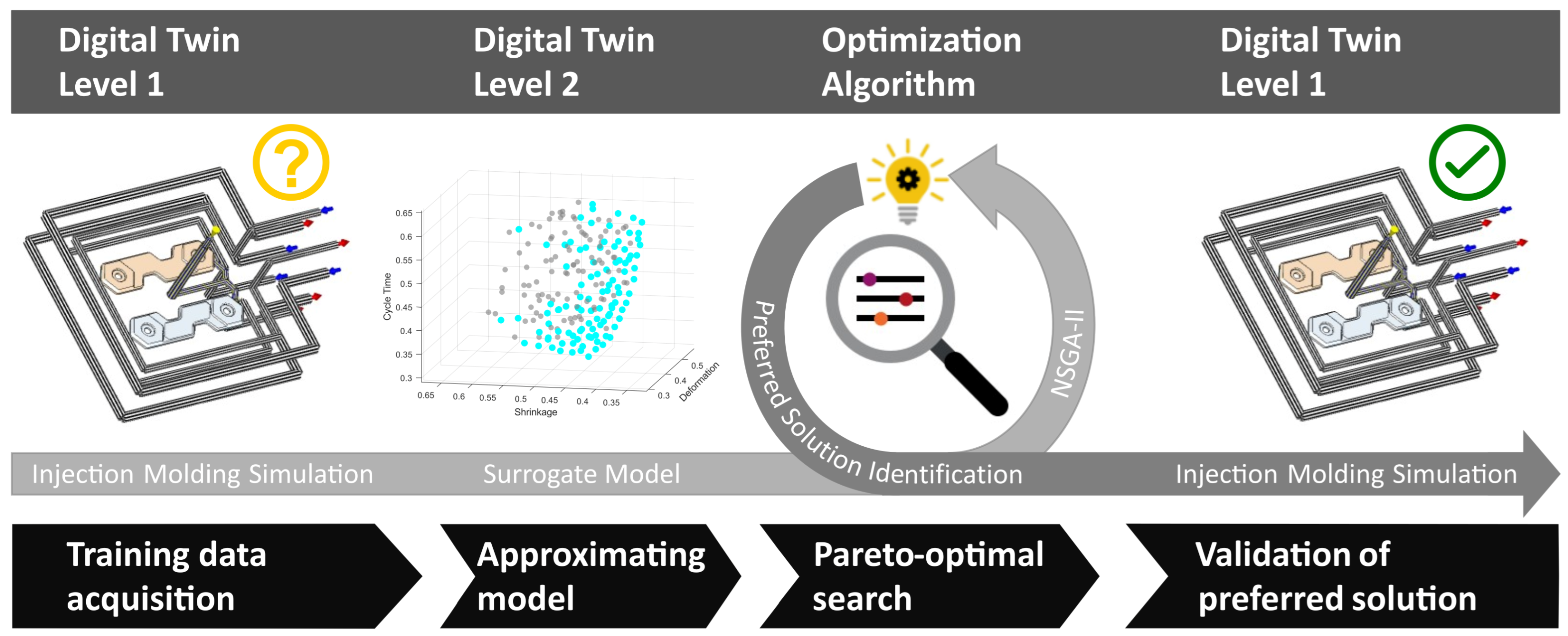
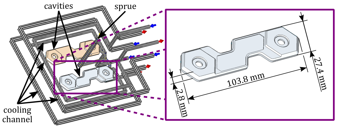
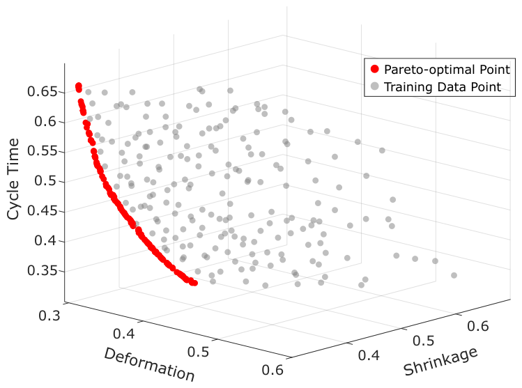
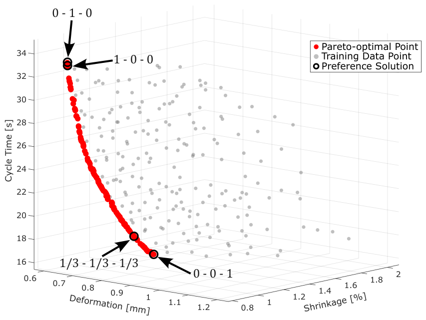
The numerical modeling of the injection molding process is implemented by using digital twins, which can be classified according to the process level. The first level of the digital twin includes the modeling of the injection molding processes with the Cadmould 3D-F injection molding simulation software. This first digital twin level is responsible for generating the training data that are required for further processing and modeling in the surrogate model. The surrogate model is subsequently used as a digital twin level 2. In this investigation, a simulation model with specific settings, e.g., geometry, material, and process parameters, is employed.

The simulation model is described as a keyholder simulation model (cf. Figure 4). This model is comparable to the structure that is used in the real production of these polymer parts. In addition to the two different cavities, the model is designed with four cooling channel geometries and a sprue for both cavities.

5.1. Modeling of Digital Twin Level 1

In the context of the numerical modeling of the digital twin level 1, the training data are typically generated by varying process parameters. This phase constitutes a significant component of the test scenario, given the limitations of existing real-world production environments for polymer parts, which prevent the manipulation of molds and polymer materials. The material properties of the polymer are given in

Table 1. Material properties of the keyholder simulation models.

Parameter	Symbol	Value
Density (melt)	${\rho }_{\mathrm{melt}}$	$702.7{\mathrm{kg}/\mathrm{m}}^3$
Density (solid)	${\rho }_{\mathrm{solid}}$	$905{\mathrm{kg}/\mathrm{m}}^3$
Specific heat capacity	$c_{p,\mathrm{polymer}}$	$2776\mathrm{J}/(\mathrm{kg}\mathrm{K})$
Thermal conductivity	${\lambda }_{\mathrm{polymer}}$	$0.1855\mathrm{W}/(\mathrm{m}\mathrm{K})$
Young’s modulus	E	$1150\mathrm{MPa}$
No-flow temperature	$T_{NF}$	$129.5 °\mathrm{C}$
Poisson’s ratio	${\nu }_P$	$0.35$
Carreau-WLF Winter	$P_1$	$459.42\mathrm{Pa}\mathrm{s}$
	$P_2$	$0.025214\mathrm{s}$
	$P_3$	$0.67191$
	$T^{*}$	$235 °\mathrm{C}$
	$T_s$	$-15.746 °\mathrm{C}$

. Specifically, the polymer PP (Borealis RF365MO) was selected for the keyholder simulation model, and all material data presented in this investigation were obtained from the Cadmould 3D-F material library. The numerical investigation is therefore limited to one thin-walled keyholder geometry and one PP material grade. This setting is used to demonstrate and analyze the complete ADEROI-based workflow under consistent modeling conditions. Consequently, the results should be interpreted as a case-specific validation of the proposed methodology rather than as an empirical proof of general applicability to arbitrary part geometries, mold configurations, or polymer materials.

The mesh is generated internally as a semi-volumetric mesh with triangular surface elements in Cadmould 3D-F. This is also referred to in the literature as an advanced 2.5D approach [54]. The mesh for the keyholder simulation model is built up with 74,151 elements and a maximum element size of 1.14 mm with a geometric volume of 14,893 mm³. The initial structure of the training data is created through an experimental design based on Latin hypercube sampling (LHS), subject to the constraint $t_{\mathrm{cooling}}>t_{\mathrm{holdingpressure}}$. This design involves the analysis of 100 valid sample points for the six input parameters that characterize the injection molding process. For reproducibility, the random number generator used for the initial LHS design was initialized with seed 0. The experimental parameters include the melt temperature $T_{\mathrm{melt}}$, holding pressure time $t_{\mathrm{holdingpressure}}$, cooling time $t_{\mathrm{cooling}}$, holding pressure $p_{\mathrm{holdingpressure}}$, volumetric flow rate during injection ${\dot{V}}_{\mathrm{injection}}$, and temperature of the cooling medium $T_{\mathrm{cooling}}$. The definition of lower limits $LB$ and upper limits $UB$ for each parameter is an essential aspect of the process, as it enables the incorporation of realistic ranges into the model (cf.

Table 2. Upper and lower limits for the LHS.

Parameter	$\mathit{LB}$	$\mathit{UB}$
$T_{\mathrm{melt}}$  ${[}^{\circ }\mathrm{C}]$	215	255
$t_{\mathrm{holdingpressure}}$  $\left[\mathrm{s}\right]$	5	15
$t_{\mathrm{cooling}}$  $\left[\mathrm{s}\right]$	10	25
$p_{\mathrm{holdingpressure}}$  $\left[\mathrm{bar}\right]$	300	500
${\dot{V}}_{\mathrm{injection}}$  $[{\mathrm{cm}}^3/\mathrm{s}]$	5	15
$T_{\mathrm{cooling}}$  ${[}^{\circ }\mathrm{C}]$	30	60

). The training data set has been generated using the LHS algorithm, which has been designed to provide a random distribution of values within the constraints of the specified parameter ranges [55]. The LHS algorithm is an effective method for maximizing the variability in input parameters, resulting in a comprehensive exploration of the parameter range.

The experimental design is simulated with Cadmould 3D-F, and the resulting data for cycle time, deformation, shrinkage, and mass are assigned to the individual tests. The cycle time $t_{\mathrm{cycle}}$ describes the total process time. It should be noted that a secondary time of $5\mathrm{s}$ is included in all simulations. In addition, the deformation $\Delta L$ can be defined as a measurable quantity that includes shrinkage and warpage. In this context, the deformation is taken to be the maximum observed deformation of the geometry. The shrinkage $V_{\mathrm{shrinkage}}$ is defined as the average reduction in the volume of the entire geometry after cooling the polymer part to the ambient temperature of 20 °C. Finally, the mass $m_{\mathrm{parts}}$ includes the weight of all polymer parts of the respective model, with the exclusion of the weight of the sprue. The experimental design is provided in the attached Appendix A.

5.2. Modeling of Digital Twin Level 2

In this contribution, the RSM model is employed as a surrogate model for the digital twin of level 2. The RSM model is used to model the process parameters in addition to creating the surrogate model. The performance is evaluated using the LOO cross-validation and HO cross-validation methods and evaluation criteria. In this context, the RMSE and the coefficient of determination $R^2$ are used as evaluation criteria. The surrogate models are implemented by converting them into so-called normalized surrogate models, which is a concept introduced as a method for modeling the surrogate models. The preparation of the normalized surrogate models first requires the mathematical normalization of the training data of the digital twin level 1. It should be noted that a precise distinction between the surrogate model and the normalized surrogate model is essential. In this contribution, the surrogate model is defined as a physical model based on the real training data set, while the normalized surrogate model is based on the normalized training data set. The modeling is necessary to achieve a harmonization of the different scales of the process parameters and target variables. The min-max scaling process is employed to normalize the data, a process which efficiently transforms the data into the interval $[0,1]$. The normalization of the variables $x_{\mathrm{norm}}$ is shown in the following equation:

$$\begin{array}{c}\hfill x_{\mathrm{norm}}={\displaystyle \frac{x-x_{\min }}{x_{\max }-x_{\min }}}\end{array}$$

(15)

This approach allows for the normalization of process parameters and objectives to the minimum values $x_{\min }$ and maximum values $x_{\max }$. This normalization guarantees that all variables x are represented on a uniform scale, improving the modeling efficiency and increasing the RSM’s convergence. Additionally, the process of normalization is used to prevent potential scale errors caused by the different scales of the variables. The normalized RSM model was approximated with a quadratic polynomial function for the regression function. The quadratic model enables the modeling of linear effects, as well as quadratic effects and interactions between the process parameters. The normalized RSM model is fitted through the least squares method. The normalization process is executed by operating within the limits specified in Table 2 for the process parameters. The objective values for the minimum parameters are set to zero, while the maximum values are defined as $2\mathrm{mm}$ for deformation, $3\%$ for shrinkage, $50\mathrm{s}$ for cycle time, and $20\mathrm{g}$ for mass.

5.3. Results of Normalized Surrogate Modeling

LOO and HO cross-validation are employed to assess the predictive accuracy and generalization capability of the normalized RSM model. In the LOO cross-validation method, each data point is iteratively excluded from the training data set, the model is retrained on the remaining data, and the excluded point is used to evaluate prediction accuracy. This process yields individual prediction errors across the data set, offering a comprehensive measure of model performance on unseen data. The resulting error metrics serve as key indicators of model reliability, highlight potential weaknesses, and inform subsequent optimization efforts.

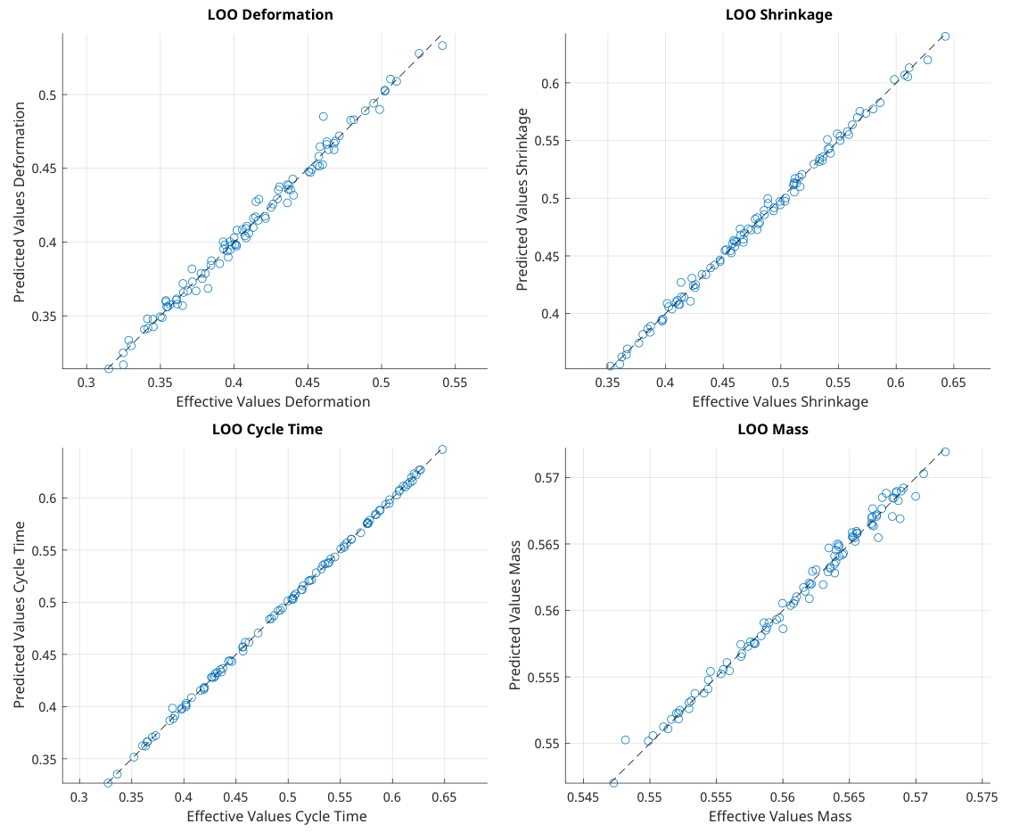
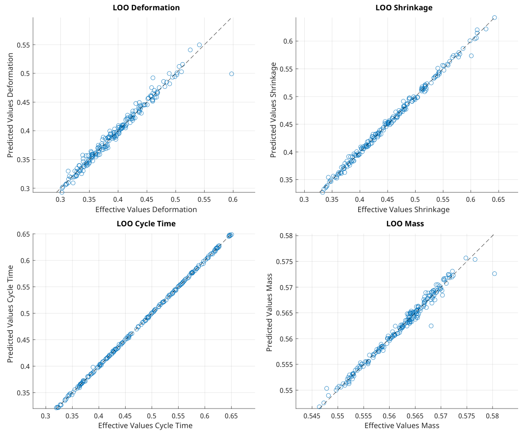
The model fit for predicting the keyholder simulation model is shown in Figure 5. The plots of the effective values compared to the predicted values demonstrate a scattering of data points, especially for higher targets, which indicates a potential decrease in the precision of these predictions. However, the figure shows that there is a significantly lower quantity of data points in the low- and high-value ranges of the objectives than in the mid-range.

In contrast, the LOO cross-validation performance indicators shown in

Table 3. LOO cross-validation performance indicators for the normalized RSM model of the keyholder simulation model.

		LOO
	Performance Indicators	Deformation	Shrinkage	Cycle Time	Mass
Normalized RSM	RMSE	0.0052	0.0041	0.0016	0.0006
	$R^2$	0.9892	0.9962	0.9996	0.9899

demonstrate high accuracy and adequate fit, as indicated by the lower RMSE values and agreement with the predicted values. The normalized RSM model consistently demonstrates low RMSE and high $R^2$ values for all objectives.

The HO cross-validation involves the separation of the data set into a training data set and a test set. The model is trained on a designated training data set and evaluated on a separate test set. This process enables the prediction of the model’s performance on unseen data [56,57,58]. For systematic evaluation, a random selection of $20\%$ of the training data set is designated as the test data set.

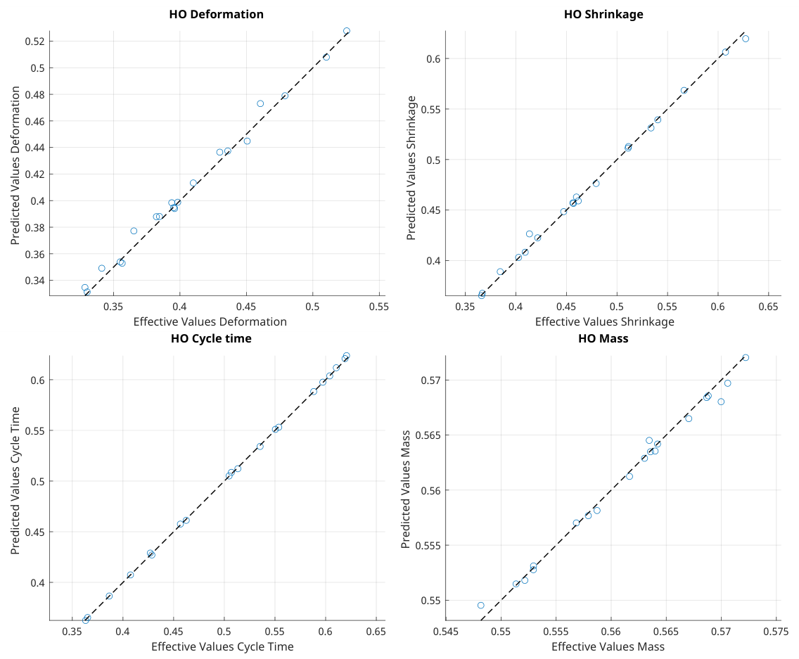
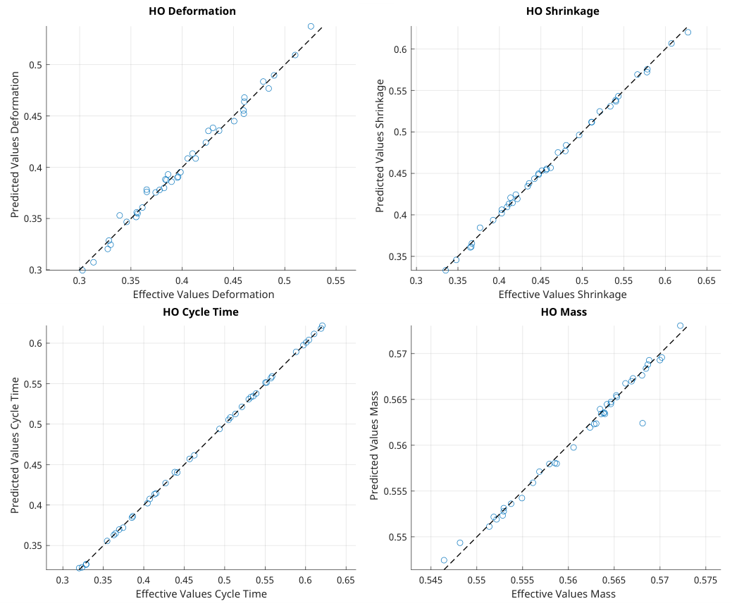
The model fit for predicting the keyholder simulation model is shown in Figure 6. A comparison of the diagrams of the effective values and the predicted values indicates a scattering of data points, particularly for higher targets. This result indicates a decrease in the precision of these predictions.

The HO cross-validation performance indicators presented in

Table 4. HO cross-validation performance indicators for the normalized RSM model of the keyholder simulation model.

		LOO
	Performance Indicators	Deformation	Shrinkage	Cycle Time	Mass
Normalized RSM	RMSE	0.0041	0.0024	0.0009	0.0007
	$R^2$	0.9904	0.9973	0.9998	0.9908

demonstrate high accuracy and adequate fit, as evidenced by the lower RMSE values and the agreement with the predicted values. The analysis of the normalized RSM model demonstrates consistently low RMSE and high $R^2$ values for all objectives.

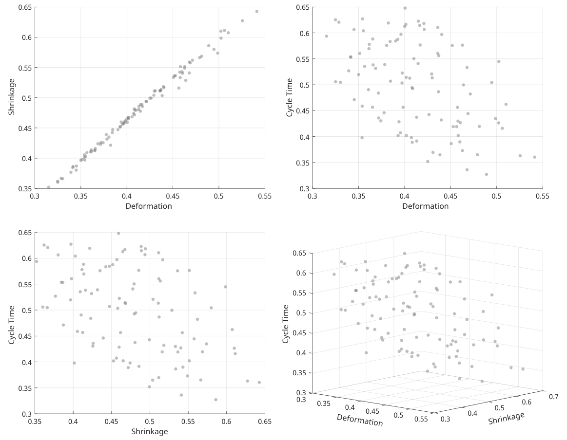
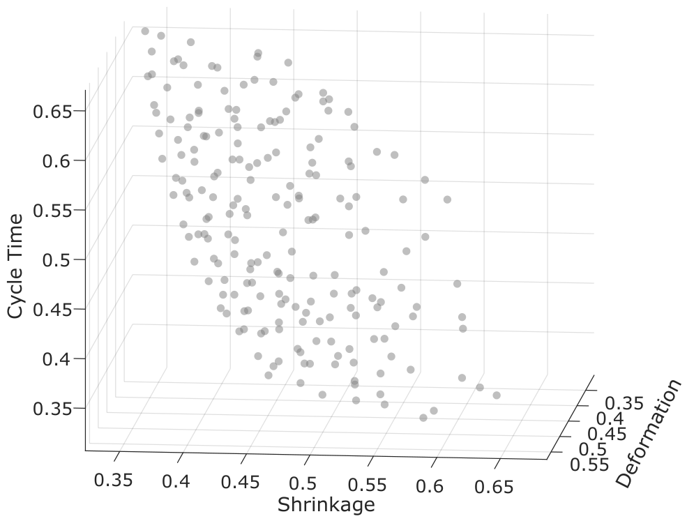
The LOO and HO cross-validation models demonstrate excellent performance indicators for the normalized RSM model, validating the models’ accuracy and the reliability of the training data set. Figure 7 shows a representation of the normalized training data from the LHS, with the objectives cycle time, shrinkage, and deformation. The plot reveals a low density of training data near the origin, which may impair the accuracy of digital twin level 2 modeling in the region critical for optimization. To improve the model fidelity in this area, a systematic enrichment of the training data set toward the origin is required.

In addition, Figure 7 indicates a strong relationship between deformation $\Delta L$ and shrinkage $V_{\mathrm{Shrinkage}}$. Therefore, an additional correlation analysis was performed for the normalized optimization objectives. Pearson correlation coefficients were calculated to quantify linear relationships, while Spearman correlation coefficients were used to assess monotonic rank correlations. The results are summarized in

Table 5. Correlation coefficients between the normalized optimization objectives of the keyholder training data set.

Correlation	$\mathbf{\Delta }\mathit{L}$ vs. ${\mathit{V}}_{\mathbf{Shrinkage}}$	$\mathbf{\Delta }\mathit{L}$ vs. ${\mathit{t}}_{\mathbf{cycle}}$	${\mathit{V}}_{\mathbf{Shrinkage}}$ vs. ${\mathit{t}}_{\mathbf{cycle}}$
Pearson	0.98816	−0.41570	−0.40336
Spearman	0.99557	−0.41479	−0.40403

.

The results confirm a strong correlation between deformation $\Delta L$ and shrinkage $V_{\mathrm{Shrinkage}}$ for the investigated keyholder case. This is consistent with the physical interpretation that the maximum deformation includes shrinkage- and warpage-related contributions. Consequently, the effective Pareto front structure is partially reduced, since improvements in shrinkage are closely linked to improvements in deformation. The strongest independent trade-off is therefore observed between the coupled quality-related objectives, deformation and shrinkage, and the process-related objective, cycle time.

Nevertheless, deformation and shrinkage are retained as separate objectives because they describe different quality aspects in injection molding. Shrinkage represents the volumetric reduction of the molded part after cooling, whereas deformation describes the maximum geometric deviation of the part and additionally includes warpage-related effects. The optimization problem is therefore kept as a three-objective formulation, while the interpretation of the resulting Pareto front explicitly accounts for the observed correlation between deformation and shrinkage.

Please note that for the investigated thin-walled keyholder case, the observed similarity between deformation and shrinkage is considered to be strongly related to the specific application scenario. Warpage still contributes to the total part deviation and therefore leads to differences between the deformation and shrinkage responses. However, for the present component and process setup, the warpage contribution is rather small compared with the shrinkage-related dimensional changes. Consequently, the maximum deformation response is mainly governed by shrinkage, which explains the very strong correlation between $\Delta L$ and $V_{\mathrm{Shrinkage}}$ in this use case. This behavior should therefore not be interpreted as a general property of injection molding optimization problems. For other geometries, wall thickness distributions, gating layouts, cooling concepts, or polymer materials, warpage-related effects may become more pronounced, and deformation and shrinkage may show a weaker correlation. The separate treatment of both quantities is therefore retained, because shrinkage and warpage contribute differently to the final part’s deviation, although shrinkage dominates the maximum deformation response in the investigated use case.

5.4. Optimization Approach for the Adaptive Expansion of the Training Data

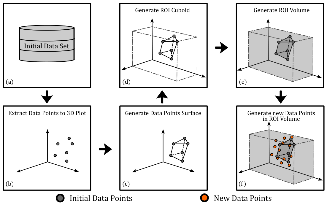
An adaptive extension of the training data set is proposed in the region of interest, guided by a surrogate model. This model systematically augments the existing data by introducing additional points toward the origin. The process for systematically expanding the training data set is shown in Figure 8.

The starting point is an existing training data set, as shown in Figure 8a. Figure 8b shows that the training data set in this example is visualized as a three-dimensional representation of the objectives to be optimized in a scatterplot. The subsequent step is shown in Figure 8c. In this step, the training data points are given a surface to create a volume. The stretching ranges $\Delta f_i=f_i^{\max }-f_i^{\min }$ for $i=1,2,3$ are subsequently calculated for each dimension, where the axis with the largest range is selected as the reference axis. This selection serves as the basis for defining upper limits in the other dimensions. By sorting the boundary points along this reference axis, interpolation functions are created that specify the maximum acceptable value as the upper limit in the other dimensions for each value of the reference axis. Based on the surface limitation, a cuboid is defined, which determines the limiting area of the ROI, as shown in Figure 8d. Since the subsequent optimization is a minimization problem, the outer points of the cuboid define the shape of the ROI. In each cuboid surface, the minimum values are used as a constant minimum value, while the maximum values of the corners are calculated from the largest expansion of the objective size data. This guarantees that all existing training data are included in the respective dimension. The resulting space is shown in Figure 8e. This space is defined by the enclosed data structure and the cuboid. It forms the real ROI, in which the known training data are separated from the unexplored region. Figure 8f shows the final step of the process. The new data points are generated based on the surrogate model, which can be specifically placed in the ROI, taking into account physical constraints as well as spatial limitations.

The specific implementation of the adaptive training data extension in the ROI method is shown using the example of the normalized surrogate model of the digital twin level 2 presented in Section 5.3. The alpha-shape method by [59] is employed to generate the surface based on the data points from Figure 7. The alpha shape approach is a methodology for representing the geometry of a point set at different levels of detail, whereby the selected parameter $\alpha$ assumes a pivotal role. When $\alpha =0$, the conventional convex hull is calculated, i.e., only the point cloud outer frame is determined. When positive values of $\alpha$ are employed, it becomes possible to approximate the outline to the data. This process emphasizes the constrictions and depressions that the convex hull would otherwise cover. Negative values of $\alpha$ direct the focus to cavity regions by employing the complement of circles, so that areas outside these circles are particularly highlighted. The method is based on the assumption that individual points are considered alpha-extreme if there is a circle with a radius of $1/\alpha$ that touches the point and, depending on the sign of $\alpha$, either includes or excludes all other points. The Delaunay triangulation of the point set is first calculated for the structured visualization of the point relationships. This triangulates the area into triangles and identifies neighboring points. The subsequent extraction of edges from the triangulation that meets the conditions for alpha-extreme points results in the creation of a triangular mesh of the point cloud, thereby generating an outer surface delineated by the mesh. This mesh not only provides a representation of the outer surface but also highlights constrictions, depressions, and inner cavities on a detailed level.

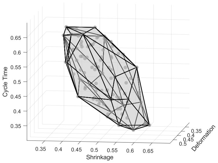
In this contribution, the training data set resulted in the selection of the parameter value of $\alpha =0$. This allows one to obtain a complete surface around the training data without inner cavities. As demonstrated in Figure 9, this factor provides sufficient structural detail of the surface of the point cloud to identify the region to be excluded.

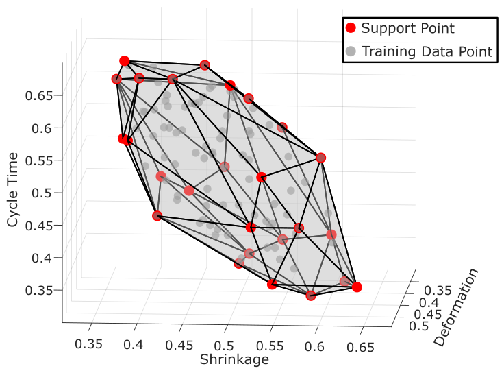
In the following, the outer corner points of the surface are defined as corner points. These corner points provide the support points for modeling an interpolation function that serves as the limiting function of the outer contour of the surfaces training data points (cf. Figure 10). In the keyholder example, the cycle time is used as the reference axis to form this interpolation function, whereby the other objectives are considered as dependent variables. The longest normalized distance between the data points in the respective axis direction defines the reference axis. In the keyholder example, the distance between the training data points in the direction of the cycle time is $\Delta f_i=0.321$.

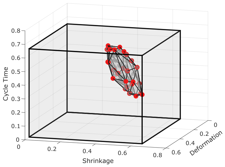
As shown in Figure 11, the generated cuboid represents the outer surface of the ROI, including the entire objective range between 0 and the respective maximum values of the training data set. Furthermore, in combination with the training data volume, this cuboid enables approximation of the real ROI.

The procedure begins with the generation of ${10}^6$ random data points in the objective space based on the surrogate model. In the second step, these data points are filtered based on their compliance with the constraints, the limits of the real ROI, and the limits of the maximum permissible values of the interpolation function of the reference axis. This filtering guarantees that only new data points located within the real ROI are retained. Subsequently, a modified greedy max-min method is employed on the filtered data points within the range of the real ROI. This method results in the selection of only 100 new data points, which are intended to complement unexplored regions and orient toward the origin. The greedy max-min approach is an iterative heuristic method used to select new points such that they are as far as possible from existing points [60]. For each new point, the minimum distance to all previously selected points is computed. The subsequent step involves the ranking of these candidate points based on their minimum distances. The selection of new points is then based on the largest minimum distances, which correspond to points that are farthest from their nearest neighboring points [60]. This iterative process is iterated until a maximum number of new points has been reached. The modified greedy max-min method employs an adapted distance metric to calculate a score $S_G\left(y\right)$. This calculation includes the original training data, a distance-to-origin penalty term, and an additional penalty term for closeness to previously observed data points. The selection of new points is based on the highest score, which is subsequently added to the training data. Furthermore, the distances are iteratively calculated based on the existing points. The score can be expressed by the following equation:

$$\begin{array}{c}\hfill S_G\left(y\right)=d_{\min }\left(y\right)-\gamma \left|\right|y\left|\right|-\delta \max \left(0,d_{\mathrm{th}}-d_{\min }\left(y\right)\right)\end{array}$$

(16)

In this equation, $d_{\min }\left(y\right)={\min }_{p\in P}\left|\right|y-p\left|\right|$ is defined as the minimum Euclidean distance from the new data point $y\in {\mathbb{R}}^n$ to all previously selected training points $P\subset {\mathbb{R}}^n$, while $\left|\right|y\left|\right|$ is the Euclidean distance to the origin. The parameter $d_{\mathrm{th}}$ is a defined threshold distance and the weighting factors $\gamma$ and $\delta$ control the influence of the penalty terms in the score calculation. The term $\max \left(0,d_{\mathrm{th}}-d_{\min }\left(y\right)\right)$ is employed to determine the inclusion of a penalty component in the score. This term is only applicable in cases where the new data point is too close in proximity to the existing training data (i.e., $d_{\min }\left(y\right)<d_{\mathrm{th}}$).

The threshold distance $d_{\mathrm{th}}$ is not interpreted as an objective spacing between the finally selected candidate points. Instead, it defines the activation range of the proximity penalty during candidate ranking. In the present implementation, $d_{\mathrm{th}}=0.5$ is selected in the normalized objective space to ensure that the proximity penalty is active for the candidate points located in the ROI. This is intentional, because the ROI represents the low-objective region in which the new candidates are expected to be selected. Thus, the threshold is used to obtain a consistent regularized ranking rule within the ROI rather than to prescribe the final nearest-neighbor distance of the selected point cloud.

For candidate points satisfying $d_{\min }\left(y\right)<d_{\mathrm{th}}$, the score can be rewritten as follows:

$$\begin{array}{c}\hfill S_G\left(y\right)=(1+\delta )d_{\min }\left(y\right)-\gamma \left|\right|y\left|\right|-\delta d_{\mathrm{th}}\end{array}$$

(17)

The last term is constant for a fixed threshold and therefore does not affect the relative ranking of candidates within the active range. Consequently, $d_{\mathrm{th}}$ primarily defines whether the proximity regularization is active, whereas $\gamma$ and $\delta$ determine the actual trade-off in the ranking. The parameter $\gamma$ controls the orientation toward the origin, while $\delta$ increases the relative weight of the distance-preserving contribution. This interpretation also explains why $d_{\mathrm{th}}$ should not be directly compared with the nearest-neighbor distances of the final selected point set. The nearest-neighbor distances characterize the local spacing between the selected candidates after the iterative selection has been completed, whereas $d_{\mathrm{th}}$ acts during the ranking of each candidate point.

In summary, this modified greedy max-min guarantees that new data points are located a considerable distance from previously obtained points, as well as having an orientation in the direction of the origin and an adequate distance to the training data.

In the keyholder simulation model example, the modified greedy max-min is implemented in normalized space. The threshold distance is set at $d_{\mathrm{th}}=0.5$, while the weighting factors $\gamma$ and $\delta$ are investigated by means of a sensitivity analysis. The limits of the LHS, as presented in Table 2, are employed as constraints during the filtration of new data points.

A quantitative analysis of the selected candidate points is performed by a density analysis of the new data point clouds in the normalized objective space. It should be noted that this analysis refers to the candidate point proposal stage before the suggested points are inversely mapped to process parameters and re-evaluated using the digital twin level 1. Therefore, surrogate accuracy indicators such as RMSE and $R^2$ are not used as primary evaluation metrics in this step. These indicators become meaningful after the proposed points have been simulated with the physics-based model and incorporated into the extended training data set. The present analysis instead isolates the influence of the point-selection parameters on the spatial distribution of the proposed candidates.

The set of new data points under consideration is defined as ${x_i}_{i=1}^n$ and the normalized objective vector as $y_i:=f^{\mathrm{norm}}\left(x_i\right)\in {[0,1]}^K$, where K is the number of objective variables. For each new data point, the distance to the nearest new data point is determined according to the following Euclidean distance:

$$\begin{array}{c}\hfill d_i=\underset{j\ne i}{min}\left|\right|y_i-y_j{\left|\right|}_2\end{array}$$

(18)

The average local density in the normalized objective space is characterized by the mean nearest neighbor distance $\overline{d_i}$.

$$\begin{array}{c}\hfill \overline{d_i}={\displaystyle \frac{1}{n}}{\displaystyle \sum _{i=1}^n}{d}_i\end{array}$$

(19)

The maximum neighbor point distance, denoted by $d_{max}$, is used to identify the largest gap in the data point cloud.

$$\begin{array}{c}\hfill d_{max}=\underset{1\le i<n}{max}{d}_i\end{array}$$

(20)

The homogeneity of the data point distances is evaluated by the standard deviation $s_d$.

$$\begin{array}{c}\hfill s_d=\sqrt{{\displaystyle \frac{1}{n-1}}\sum _{i=1}^n{(d_i-\overline{d_i})}^2}\end{array}$$

(21)

Based on the interpretation of $d_{\mathrm{th}}$ as an activation threshold, the sensitivity analysis focuses on the two weighting parameters $\gamma$ and $\delta$, which directly control the trade-off between orientation toward the origin and distance-preserving regularization. A factorial design with $\gamma \in \{0,0.1,0.2\}$ and $\delta \in \{0,1,2\}$ is investigated. For each parameter combination, 100 candidate points are selected in the ROI and evaluated using $\overline{d_i}$, $d_{max}$, and $s_d$. The results are summarized in

Table 6. Sensitivity analysis of the modified greedy max-min criterion.

No.	$\mathit{\gamma }$	$\mathit{\delta }$	$\overline{{\mathit{d}}_{\mathit{i}}}$	${\mathit{d}}_{max}$	${\mathit{s}}_{\mathit{d}}$
1	0	0	0.000452	0.001405	0.000295
2	0	1	0.000452	0.001405	0.000295
3	0	2	0.000452	0.001405	0.000295
4	0.1	0	0.000459	0.006570	0.000767
5	0.1	1	0.000470	0.003445	0.000440
6	0.1	2	0.000471	0.002456	0.000399
7	0.2	0	0.000294	0.001333	0.000249
8	0.2	1	0.000460	0.006569	0.000767
9	0.2	2	0.000461	0.003798	0.000451

.

The results show that the orientation parameter $\gamma$ has a stronger influence on the point selection behavior than the proximity weight $\delta$. For $\gamma =0$, all three variants identical values for $\overline{d_i}$, $d_{max}$, and $s_d$. In this case, the origin-oriented term is inactive and the selection behavior corresponds to the classical distance-based greedy max-min strategy. The value of $\delta$ has no effect in this configuration, because the proximity penalty does not change the ranking of the candidate points when no orientation toward the origin is introduced.

Introducing a moderate orientation with $\gamma =0.1$ changes the selection behavior. Without the proximity penalty, $d_{max}$ and $s_d$ increase noticeably, which indicates that the selected points are shifted toward the ROI, while the distribution becomes less homogeneous. The combination $\gamma =0.1$ and $\delta =1$ reduces both $d_{max}$ and $s_d$ while maintaining a comparable mean nearest-neighbor distance. This indicates a balanced candidate distribution with ROI-oriented enrichment and reduced local irregularity. A further increase to $\delta =2$ slightly reduces $d_{max}$ and $s_d$, but the improvement is comparatively small. Therefore, $\delta =1$ is selected as a moderate regularization weight that avoids excessive weighting of the proximity penalty.

A stronger orientation with $\gamma =0.2$ does not provide a clear improvement. In the case of $\delta =0$, the mean nearest-neighbor distance decreases markedly, which indicates a stronger local concentration of candidate points. For $\delta =1$ and $\delta =2$, the distribution metrics are comparable to the case $\gamma =0.1$, but without a distinct improvement in homogeneity or coverage. Consequently, $\gamma =0.1$ is selected as a moderate orientation weight that directs the candidate selection toward the relevant ROI without causing excessive local concentration.

Based on this sensitivity analysis, the parameter combination $\gamma =0.1$, $\delta =1$, and $d_{\mathrm{th}}=0.5$ is used for the modified greedy max-min criterion. This combination provides a balanced compromise between distance-based exploration, orientation toward the origin, and controlled avoidance of candidate clustering near previously sampled regions. The main parameter settings used for ADEROI are given in Appendix A 

Table A2. Main parameter settings used for the ADEROI-based training data extension.

Parameter	Value
Initial LHS sample size	100
Number of ROI candidate points	${10}^6$
Number of added ADEROI points	100
Alpha shape parameter $\alpha$	0
Threshold distance $d_{\mathrm{th}}$	0.5
Origin-orientation weight $\gamma$	0.1
Distance-preservation weight $\delta$	1
Random seed for ROI candidate generation	0

.

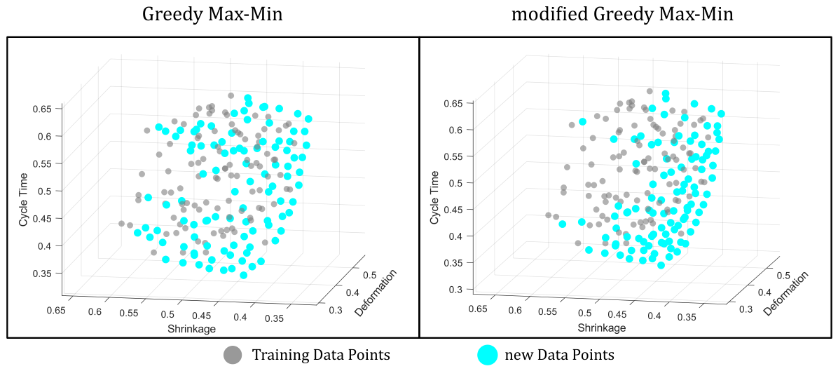
The results of the distributions of the classical greedy max-min approach and the selected modified greedy max-min approach are shown in Figure 12. It is important to note that in the classic greedy max-min approach, the original training data are also taken into account when selecting new data points. This allows for a comparison between the unmodified distance-based selection and the final ADEROI point selection using $\gamma =0.1$, $\delta =1$ and $d_{\mathrm{th}}=0.5$. The figure shows that the modified greedy max-min approach results in a significantly better orientation in the direction of the origin when selecting the new data points. In addition, this approach allows the orientation of the solution region to be developed in the direction of the ideal optimum. In this region, a significant compression with an equivalent quantity of 100 new data points can be observed. This can result in an improved quality of the surrogate model in the potential optimal solution region during a subsequent validation of these new data points.

In summary, the application to the keyholder simulation model shows that the adaptive training data extension in the ROI (ADEROI) in combination with the modified greedy max-min provides a structured candidate point selection in the possible optimal solution region. It is important to note that the inclusion of new data points is intended to serve as a suggestion for the structured approximation of the solution region. Due to the potential inaccuracy of the surrogate model, it is necessary to calculate the data points using the digital twin level 1 before further analysis.

5.5. Results of the Extended Normalized Surrogate Modeling

The data points determined with ADEROI and the modified greedy max-min approach for an extension of the digital twin level 2 can be applied if the process parameters are calculated inversely by the surrogate model and simulated with the digital twin level 1. However, due to the potential inaccuracy of the surrogate model, the results simulated with the digital twin level 1 could differ slightly from the suggested new data points. As shown in Figure 13, the new training data set, based on the original training data set of the LHS and the new simulated data set, clearly demonstrates the clustering of valid test points for the extended normalized surrogate model in the region of a potential optimal solution in the direction of the origin.

The model fit for predicting the keyholder simulation model with the new training data set is shown in Figure 14 and Figure 15. The diagrams of the effective values compared to the predicted values show a scatter in the comparison of the new training data points with the original data points. The LOO cross-validation diagrams for the deformation and mass show individual outliers in the higher-value range, whereas a compression of the data points in the low-value range is evident (cf. Figure 14). In contrast, the cycle time shows a consistent compression of data points in the mid-range, while the mass shows a more pronounced, concentrated density of data points in the mid-range.

In the context of HO cross-validation, a random selection of $20\%$ of the new training data set was designated as the new test data set (cf. Figure 15). The diagram also demonstrates a strong correlation between the effective values and the predictive values. The HO cross-validation demonstrates comparable performance in predicting points based on the remaining $80\%$ of the new training data points.

As shown in

Table 7. LOO and HO cross-validation performance indicators for the extended normalized RSM model of the keyholder simulation model.

		LOO
	Performance Indicators	Deformation	Shrinkage	Cycle Time	Mass
Normalized RSM	RMSE	0.0052	0.0041	0.0016	0.0006
	$R^2$	0.9892	0.9962	0.9996	0.9899
Extended normalized RSM	RMSE	0.0095	0.0045	0.0013	0.0009
	$R^2$	0.9683	0.9958	0.9998	0.9783
		HO
	Performance indicators	Deformation	Shrinkage	Cycle Time	Mass
Normalized RSM	RMSE	0.0041	0.0024	0.0009	0.0007
	$R^2$	0.9904	0.9973	0.9998	0.9908
Extended normalized RSM	RMSE	0.0047	0.0027	0.0008	0.0005
	$R^2$	0.9885	0.9979	0.9999	0.9765

, the LOO and HO cross-validation performance indicators for the normalized RSM model and the extended normalized RSM model are presented. This table also presents the data for the normalized RSM model from Table 3 and Table 4 to enhance clarity. The extended normalized RSM model shows a minimal decrease in the performance indicators for deformation, shrinkage, and mass. The cycle time showed marginal improvement in comparison with the normalized RSM model. However, it can be concluded that these variations are minimal and that the extended normalized RSM model is a good fit.

In summary, it can be concluded that the proposed extended normalized RSM is characterized by a significantly enhanced data set, focusing in the direction of the assumed optimum in the solution space. The surrogate model can approximate this region without significant gaps due to missing data points. The enhancement is deliberately ROI-focused and new data points are placed in decision-relevant neighborhoods of the Pareto front. As a result, global cross-validation metrics may change only marginally, or even decrease slightly, because the added samples probe more challenging parts of the response surface. This behavior reflects a standard bias–variance trade-off and is consistent with our goal of improving decision quality within the ROI.

5.6. Budget-Controlled Retrospective Benchmark

The following benchmark is intended as a retrospective comparison against a scaled single-stage LHS baseline. It evaluates whether the ROI-directed enhancement by ADEROI with modified greedy max-min reaches an equivalent ROI point density with fewer simulation runs than an unguided LHS expansion for the investigated keyholder case. The benchmark does not claim superiority over established sequential sampling strategies such as expected improvement (EI), probability of improvement (PI), upper confidence bound (UCB), or expected hypervolume improvement (EHVI). A methodologically fair comparison with these acquisition strategies requires separate sequential sampling workflows under harmonized computational budgets, including re-evaluation of the proposed points with digital twin level 1, surrogate refitting and a joint assessment of ROI density, surrogate accuracy, and total simulation runtime. Such a comparison is therefore treated as a dedicated benchmark study and is identified as future work.

Within this retrospective LHS-baseline benchmark, the ROI-directed enhancement (ADEROI with modified greedy max-min) is compared against a larger one-shot LHS design. In the context of comparable ROI point density, the present analysis aims to quantify the number of additional LHS simulations required to achieve a point density comparable to ADEROI within the decision-relevant ROI. This approach enables the estimation of savings in simulations and a conservative reduction in simulation time. The measurements were performed on a workstation with a 3 GHz Intel Xeon Gold 6248R CPU (48 cores) and 383 GB RAM, using Cadmould 3D-F V16.1 and MATLAB R2024b.

The comparison is based exclusively on the existing 200 simulated points (100 LHS and 100 ADEROI ROI points). The normalization of the objectives is outlined in Section 5.2. The density analysis is based on the consistent computation of nearest-neighbor distances in the normalized objective space within the ROI, resulting in ${\overline{d}}_{\mathrm{LHS}}=0.00032$ for the 100 LHS points with an enclosed volume $V_{\mathrm{LHS}}=0.000349$ and ${\overline{d}}_{\mathrm{ROI}}={\overline{d}}_{\mathrm{target}}=0.00033$ for the 100 ROI points with an enclosed volume $V_{\mathrm{ROI}}=0.000502$. The total volume that a scaled-up LHS would need to cover is approximated by the volume of the hull of the union of both point sets ${\mathcal{P}}_{•}$, i.e., $V\left(\mathrm{hull}({\mathcal{P}}_{\mathrm{LHS}}\cup {\mathcal{P}}_{\mathrm{ROI}})\right)$. The convex hull is used consistently for all volumes. This results in $V_{\mathrm{target}}=0.001258$.

In an M-dimensional normalized objective space, a characteristic length scale (e.g., the average nearest-neighbor distance) scales with the sample size as $\overline{d}\propto {\left({\displaystyle \frac{V}{n}}\right)}^{1/M}$. The ROI-equivalent LHS sample size $n_{\mathrm{eq}}$ that attains the same point density as the 100 ROI points can be determined using the following equation:

$$n_{\mathrm{eq}}=n_{\mathrm{LHS}}{\displaystyle \frac{V_{\mathrm{target}}}{V_{\mathrm{LHS}}}}{\left({\displaystyle \frac{{\overline{d}}_{\mathrm{LHS}}}{{\overline{d}}_{\mathrm{target}}}}\right)}^M$$

(22)

The additional number of LHS points relative to the designated 200-point budget is determined by the following equation:

$$\Delta n=n_{\mathrm{eq}}-200$$

(23)

The conservative time reduction is computed from the average simulation time per run $t_{\mathrm{sim}}$, the effective parallelism P, and the ADEROI selection overhead $t_{\mathrm{ADEROI}}$, by the following equation:

$$\Delta t={\displaystyle \frac{\Delta n·t_{\mathrm{sim}}}{P}}-t_{\mathrm{ADEROI}}$$

(24)

With the LHS reference sample size $n_{\mathrm{LHS}}=100$ and $M=3$, it can be obtained that $\Delta n=129$. By using $t_{\mathrm{sim}}=1687\mathrm{s}$, $P=5$, and $t_{\mathrm{ADEROI}}=38\mathrm{s}$, the corresponding time saving is $\Delta t=12.05\mathrm{h}$ compared to an ROI-equivalent LHS. The associated runtimes are $t_{\mathrm{LHS},\mathrm{eq}}={\displaystyle \frac{n_{\mathrm{eq}}·t_{\mathrm{sim}}}{P}}=30.84\mathrm{h}$ and $t_{\mathrm{framework}}={\displaystyle \frac{200·t_{\mathrm{sim}}}{P}}+t_{\mathrm{ADEROI}}=18.76\mathrm{h}$, which define the speed-up by the following equation:

$$\mathrm{speed}-\mathrm{up}={\displaystyle \frac{t_{\mathrm{LHS},\mathrm{eq}}}{t_{\mathrm{framework}}}}=1.64$$

(25)

In comparison to an ROI-equivalent LHS, the proposed ADEROI method with modified greedy max-min reduces runtime from $30.84\mathrm{h}$ to $18.76\mathrm{h}$ ($-39.1\%$) and achieves a 1.64× speed-up. These efficiency values refer exclusively to the scaled LHS baseline and the investigated keyholder data set. They should therefore be interpreted as a case-specific LHS-baseline result rather than as a general performance comparison against other adaptive or Bayesian sequential sampling methods.

6. Optimization of the Digital Twin Level 2

The optimization of the digital twin level 2 is based on the previously identified extended normalized RSM model. Since the optimization is performed on the surrogate representation of digital twin level 1, the optimizer acts exclusively on the normalized RSM-based objective functions and constraints. Before the final optimizer is used for the subsequent preference-driven solution identification, a compact benchmark of classical multi-objective optimizers is performed to quantify the Pareto front quality under identical surrogate model conditions.

The optimization problem for the keyholder simulation model can be described as follows:

$$\begin{array}{c}\hfill \underset{x\in {\mathbb{R}}^n}{\min },f(\Delta L\left(x\right),V_{\mathrm{Shrinkage}}\left(x\right),t_{\mathrm{cycle}}\left(x\right))\hfill \\ \\ \hfill \begin{array}{ccc}\hfill \mathrm{s}.\mathrm{t}.\Delta L\left(x\right)& \le \hfill & 1\mathrm{mm}\hfill \\ \hfill V_{\mathrm{shrinkage}}\left(x\right)& \le \hfill & 1.5\%\hfill \\ \hfill m_{\mathrm{parts}}\left(x\right)& \ge \hfill & 11\mathrm{g}\hfill \\ \hfill t_{\mathrm{holdingpressure}}& <\hfill & t_{\mathrm{cooling}}\hfill \\ \hfill 215 °\mathrm{C}& \le \hfill & T_{\mathrm{melt}}\le 255 °\mathrm{C}\hfill \\ \hfill 5\mathrm{s}& \le \hfill & t_{\mathrm{holdingpressure}}\le 15\mathrm{s}\hfill \\ \hfill 10\mathrm{s}& \le \hfill & t_{\mathrm{cooling}}\le 25\mathrm{s}\hfill \\ \hfill 300\mathrm{bar}& \le \hfill & p_{\mathrm{holdingpressure}}\le 500\mathrm{bar}\hfill \\ \hfill 5{\mathrm{cm}}^3/\mathrm{s}& \le \hfill & {\dot{V}}_{\mathrm{injection}}\le 15{\mathrm{cm}}^3/\mathrm{s}\hfill \\ \hfill 30 °\mathrm{C}& \le \hfill & T_{\mathrm{cooling}}\le 60 °\mathrm{C}\hfill \end{array}\hfill \end{array}$$

(26)

It is important to note that only the deformation $\Delta L\left(x\right)$, shrinkage $V_{\mathrm{Shrinkage}}\left(x\right)$, and cycle time $t_{\mathrm{cycle}}\left(x\right)$ objectives are considered in the minimization problem. The objective of mass $m_{\mathrm{parts}}\left(x\right)$ is regarded as a constraint during the optimization problem. The digital twin level 1 employed establishes the relationship $t_{\mathrm{holdingpressure}}<t_{\mathrm{cooling}}$, since the cooling time $t_{\mathrm{cooling}}$ includes the holding pressure time $t_{\mathrm{holdingpressure}}$. The limits of the LHS were used as the limits of the constraints for the process parameters.

6.1. Surrogate-Based Optimizer Benchmark

To address the Pareto front quality beyond the convergence curves, NSGA-II, MOPSO, and MOEA/D are compared on the extended normalized RSM model. The comparison is performed on digital twin level 2, since this is the objective function representation used by the optimization algorithm in the proposed workflow. This setup isolates the influence of the optimizer while keeping the surrogate model, objective functions, constraints, and normalization limits identical. All three algorithms are executed with the same population size of $N=200$ and the same maximum number of generations $G_{max}=200$, resulting in an identical budget of $N·G_{max}=40,000$ surrogate model evaluations per run. To account for stochastic variability, 10 independent runs are performed for each algorithm.

This fixed-budget benchmark is used only for the comparative Pareto front quality assessment and is separated from the final NSGA-II workflow, which uses the convergence criteria described in Section 6.2.

To improve reproducibility, the main hyperparameters and random number seed settings used for the optimizer benchmark are summarized in

Table 8. Hyperparameters and random number seed settings used for the RSM-based optimizer benchmark.

Algorithm	Parameter	Value
All	Population size N	200
All	Maximum number of generations $G_{max}$	200
All	Number of independent runs	10
All	Evaluation budget per run	40,000
NSGA-II	Crossover probability $p_c$	0.3
NSGA-II	Mutation probability $p_m$	$1/6$
NSGA-II	SBX distribution index ${\eta }_c$	20
NSGA-II	Random seeds	$1,\dots ,10$
MOPSO	Inertia factor $\chi$	0.4
MOPSO	Cognitive acceleration coefficient $c_1$	1.5
MOPSO	Social acceleration coefficient $c_2$	1.5
MOPSO	Archive size	200
MOPSO	Mutation probability $p_m$	$1/6$
MOPSO	Mutation range	0.05
MOPSO	Random seeds	$1001,\dots ,1010$
MOEA/D	Number of neighbors T	20
MOEA/D	Neighborhood selection probability $\delta$	0.9
MOEA/D	Differential evolution factor F	0.5
MOEA/D	Crossover rate $CR$	1.0
MOEA/D	Mutation probability $p_m$	$1/6$
MOEA/D	Mutation range	0.05
MOEA/D	Random seeds	$2001,\dots ,2010$

. The benchmark runs use fixed population sizes and fixed maximum generation numbers to ensure a comparable evaluation budget across all algorithms. The random seeds are assigned deterministically for the independent runs.

The Pareto front quality is evaluated using HV and IGD in the normalized objective space. The common hypervolume reference point is set to $r^{\mathrm{HV}}={(1.1,1.1,1.1)}^{\top }$, which is dominated by the relevant non-dominated solutions in the normalized minimization problem. The IGD reference front ${\mathcal{P}}_{\mathrm{ref}}$ is constructed from the non-dominated union of the final Pareto fronts obtained by NSGA-II, MOPSO, and MOEA/D over all benchmark runs. This procedure provides a common approximation of the best available Pareto front and ensures that all algorithms are assessed under identical quality criteria. In

Table 9. RSM-based Pareto front quality benchmark of NSGA-II, MOPSO, and MOEA/D. HV and IGD are calculated in the normalized objective space.

Algorithm	HV	${\mathit{\sigma }}_{\mathbf{HV}}$	IGD	${\mathit{\sigma }}_{\mathbf{IGD}}$	${\mathit{N}}_{\mathbf{PF}}$
NSGA-II	0.46819	0.00084	0.00452	0.00055	$129.1\pm 7.16$
MOPSO	0.47052	0.00050	0.00192	0.00018	$200.0\pm 0.00$
MOEA/D	0.46885	0.00073	0.00578	0.00058	$192.0\pm 1.76$

, the results of the RSM-based Pareto front quality benchmark of NSGA-II, MOPSO, and MOEA/D are presented. The calculation of HV and IGD is performed in the normalized objective space, while ${\sigma }_{\mathrm{HV}}$ and ${\sigma }_{\mathrm{IGD}}$ represent the corresponding standard deviations.

The benchmark shows that all three algorithms achieve comparable hypervolume values on the extended normalized RSM model. MOPSO obtains the highest HV and the lowest IGD, indicating the largest dominated objective-space region and the densest approximation of the joint reference front. MOEA/D achieves a slightly higher HV than NSGA-II, but it also shows the highest IGD among the three algorithms. This indicates that MOEA/D reaches a comparable dominated objective-space region, but its approximation of the joint reference front is less accurate in terms of average distance and coverage. NSGA-II achieves an HV of 0.46819, which is close to MOPSO with an absolute difference of 0.00233 and close to MOEA/D with an absolute difference of 0.00066. Relative to the best HV value obtained by MOPSO, the difference is approximately $0.5\%$. Thus, the dominated objective-space region obtained by NSGA-II is nearly equivalent to the best-performing benchmark result.

The IGD values provide additional information on the density and coverage of the Pareto front approximation. MOPSO retains $200.0\pm 0.00$ non-dominated solutions and therefore provides the densest representation of the joint reference front. NSGA-II produces $129.1\pm 7.16$ Pareto points on average and consequently shows a higher IGD than MOPSO. MOEA/D generates $192.0\pm 1.76$ Pareto points on average, but its IGD remains higher than that of NSGA-II. This indicates that the number of non-dominated points alone is insufficient to characterize the quality of the approximation. While MOPSO provides the best coverage of the joint reference front, NSGA-II offers a balanced performance with a nearly equivalent HV and a lower IGD than MOEA/D.

Based on this benchmark, NSGA-II is selected as the main optimizer for the subsequent preference-driven optimization workflow. Although MOPSO achieves the best numerical values for HV and IGD, the improvement in HV over NSGA-II is small, whereas the main advantage of MOPSO is the denser sampling of the approximated front. For the present study, the objective is not to generate the densest possible Pareto front representation, but to obtain a representative, diverse, and well-established set of trade-off solutions for subsequent preference-based decision making. NSGA-II fulfills this requirement while providing a dominated objective-space region that is nearly equivalent to the best benchmark result and an IGD that is better than that of MOEA/D. In addition, NSGA-II is a widely established reference method in surrogate-based and injection-molding-related multi-objective optimization. Therefore, the benchmark supports the use of NSGA-II as a methodologically appropriate optimizer for the proposed workflow.

Consequently, the benchmark is interpreted as a Pareto front quality assessment and robustness check on digital twin level 2, while NSGA-II is selected for the final optimization chain. This preserves consistency with the subsequent preference-based selection and the validation of selected operating points with digital twin level 1.

6.2. NSGA-II Optimization and Convergence Behavior

Based on the benchmark and the subsequent optimizer selection, the NSGA-II is used for the final optimization of the digital twin level 2. The NSGA-II is employed in conjunction with the previously described genetic operators and the crowding distance. The optimization process involves the introduction of two convergence metrics. The first is used to evaluate the orientation of the Pareto front with reference to the theoretical optimum at the origin and is called the reference distance. The second convergence metric is used to guarantee diversity by adjusting the population size and is called diversity. The definitions of these two convergence measures are described as follows.

The convergence metric of the reference distance is defined as the Euclidean distance between the origin and the nearest reference point on the Pareto front, determined in the respective generation. The difference between the current generation’s reference distance and the previous generation’s reference distance is used to calculate the convergence behavior between the generations. Should the difference between the reference distance of the current generation $d_t$ and the reference distance of the previous generation $d_{t-1}$ be less than a defined threshold value ${ϵ}_{\mathrm{ref}}$ over a specified number of generations $G_{\mathrm{ref}}$, the stop criterion for the reference distance is applied. The convergence relationship of the reference distance is shown in the following equation:

$$\begin{array}{c}\hfill |d_t-d_{t-1}|<{ϵ}_{\mathrm{ref}}\end{array}$$

(27)

The convergence metric of diversity is employed to regulate the size of generations, with diversity defined as the pairwise Euclidean distance between individuals in a respective generation. The difference between the pairwise Euclidean distances of the current generation $D_t$ and the pairwise Euclidean distances of the previous generation $D_{t-1}$ is used as a reference value for the threshold value ${ϵ}_{\mathrm{div}}$. The population size is increased by $10\%$, under the assumption that the difference is less than a defined threshold and considering a defined number of generations $G_{\mathrm{div}}$. The number of generations, which serves as a stop criterion, can also be interpreted as a threshold value. If no expansion has occurred over this number of generations, the stop criterion for the diversity is applied. The diversity can be expressed by the following equation:

$$\begin{array}{c}\hfill |D_t-D_{t-1}|<{ϵ}_{\mathrm{div}}\end{array}$$

(28)

The following equation describes the pairwise Euclidean distance. The pairwise Euclidean distance $D_t$ is defined as the average of all pairwise Euclidean distances in a generation. In this equation, $d(x_j,x_k)$ describes the Euclidean distance between the individuals and n is the number of individuals in the generation.

$$\begin{array}{c}\hfill D_t={\displaystyle \frac{2}{n(n-1)}}{\displaystyle \sum _{j=1}^{n-1}}{\displaystyle \sum _{k=j+1}^n}d(x_j,x_k)\end{array}$$

(29)

The NSGA-II is stopped based on the convergence metrics for the reference distance and the diversity, resulting in the final generation being used as a valid Pareto-optimal solution set.

The normalized convergence criteria of the keyholder simulation model were set to ${ϵ}_{\mathrm{ref}}={10}^{-5}$ for the reference distance and ${ϵ}_{\mathrm{div}}={10}^{-2}$ for the diversity. For the final NSGA-II optimization, the random number generator was initialized with seed 0. The crossover probability was set to $p_c=0.3$, the mutation probability to $p_m=1/6$, and the SBX distribution index to ${\eta }_c=20$. The number of generations for both convergence metrics is $G_{\mathrm{ref}}=G_{\mathrm{div}}=8$. The initial population size was set at 200 individuals, and the final population size was identified as 220 individuals. The convergence metrics were obtained after 403 generations, and a total of 191 Pareto-optimal solutions were determined.

The convergence behavior of the normalized reference distances and the diversity is shown in Figure 16. The plot of the reference distance shows the progress of the convergence of the solutions to the origin. It is shown that there is a continuous improvement or convergence of the solutions for the distance to the reference point until the threshold is reached. The diversity metric, calculated as the average of the pairwise distances of the normalized target values, shows a slight increase in diversity over the generations or, respectively, a convergence to a constant value. This indicates a good balance between exploration (diversity) and exploitation (focus on potential regions).

The normalized Pareto front generated by the NSGA-II based on the extended normalized RSM model is shown in Figure 17. The results indicate that the Pareto-optimal points in the normalized space are located in a slightly different region than in the original extended training data. The figure presents the convex approximation of the Pareto front for the keyholder simulation model. It is evident that ADEROI, in combination with the modified greedy max-min approach, has significantly increased the density of the training data points in the solution space of the Pareto front without previously identifying a possible gap between the Pareto front and the training data. Therefore, an improved modeling of the normalized RSM with the previously proposed method can be derived since gaps in the definition regarding the possible solution front could already be closed based on the initial digital twin level 2. Additionally, the implementation of convergence metrics effectively guarantees the orientation and diversity of the Pareto front.

In accordance with the correlation analysis in Section 5.3, the Pareto front should be interpreted as an effectively reduced trade-off structure for the investigated case, mainly balancing the coupled quality-related objectives $\Delta L$ and $V_{\mathrm{Shrinkage}}$ against the process-related objective $t_{\mathrm{cycle}}$.

7. Preferred Solution Identification Method

Multi-objective optimization with the NSGA-II approach includes extensive solution identification by generating many Pareto-optimal solutions. A preferred solution identification method is proposed for systematic solution identification. This method is predicated on the methodical preference of rated Pareto-optimal solutions. A weighted sum of the respective normalized objectives is calculated as part of the preferred solution identification method. The weightings are used to integrate the preference for a specific objective. The result of this weighting is referred to as the score. This calculation of the score allows for the identification of the lowest score as the preferred Pareto-optimal solution. The following equation is employed to calculate the score:

$$\begin{array}{c}\hfill \mathrm{Score}={\displaystyle \sum _{i=1}^n}{w}_i{f}_i\left(x\right)\mathrm{with}{w}_i\in [0,1]\mathrm{and}{\displaystyle \sum _{i=1}^n}{w}_i\stackrel{!}{=}1\end{array}$$

(30)

In this equation, $w_i$ is the weighting of each normalized objective $f_i\left(x\right)$. According to this approach, the restriction of the sum of the weightings allows an equal preference for a large number of objectives. A high weighting of an objective corresponds to increased consideration of that objective. In contrast, lower weightings result in lower consideration of the respective preference in the score. This method enables a preference-oriented choice of the most preferable Pareto-optimal solution. The weighted sum approach is characterized by its transparency and its application-oriented nature for industrial practice in decision making. It is important to note that non-convex areas of the Pareto set may be underrepresented as a result.

In the keyholder simulation model example, four possible preference scenarios are analyzed. In this analysis, $w_1$ corresponds to the weighting of the deformation, $w_2$ to the weighting of the shrinkage, and $w_3$ to the weighting of the cycle time. The overall preference is specified according to the definition $w_1-w_2-w_3$, taking into account the three optimized objectives.

This contribution defines four preference scenarios according to the weighting constellation. The four preference scenarios are determined by considering each objective as the dominant preference variable ($1-0-0$, $0-1-0$, and $0-0-1$) and one scenario where each objective is equally weighted ($1/3-1/3-1/3$). The identified solutions using the preferred solution identification method are shown in Figure 18.

The respective process parameters are identified from the preference solutions by inverse determination based on the surrogate model.

Table 10. Preference optimal solutions and inverse determined process parameters for the keyholder simulation model.

Preference Weighting	$1-0-0$	$0-1-0$	$0-0-1$	$1/3-1/3-1/3$
$\Delta L\left(x\right)$	$0.58\mathrm{mm}$	$0.59\mathrm{mm}$	$0.75\mathrm{mm}$	$0.71\mathrm{mm}$
$V_{\mathrm{Shrinkage}}\left(x\right)$	$0.98\%$	$0.97\%$	$1.29\%$	$1.21\%$
$t_{\mathrm{cycle}}\left(x\right)$	$32.8\mathrm{s}$	$32.85\mathrm{s}$	$16.23\mathrm{s}$	$17.82\mathrm{s}$
$m_{\mathrm{parts}}$	$11.41\mathrm{g}$	$11.39\mathrm{g}$	$11.38\mathrm{g}$	$11.42\mathrm{g}$
$T_{\mathrm{melt}}$	$248.9 °\mathrm{C}$	$254.7 °\mathrm{C}$	$215.4 °\mathrm{C}$	$215 °\mathrm{C}$
$t_{\mathrm{holdingpressure}}$	$12.1\mathrm{s}$	$11.9\mathrm{s}$	$9.5\mathrm{s}$	$11\mathrm{s}$
$t_{\mathrm{cooling}}$	$25\mathrm{s}$	$25\mathrm{s}$	$10\mathrm{s}$	$11.7\mathrm{s}$
$p_{\mathrm{holdingpressure}}$	$500\mathrm{bar}$	$500\mathrm{bar}$	$500\mathrm{bar}$	$500\mathrm{bar}$
${\dot{V}}_{\mathrm{injection}}$	$5.2{\mathrm{cm}}^3/\mathrm{s}$	$5{\mathrm{cm}}^3/\mathrm{s}$	$12{\mathrm{cm}}^3/\mathrm{s}$	$14.3{\mathrm{cm}}^3/\mathrm{s}$
$T_{\mathrm{cooling}}$	$30 °\mathrm{C}$	$30 °\mathrm{C}$	$30 °\mathrm{C}$	$30 °\mathrm{C}$

presents the identified process parameters and their corresponding objectives.

The preferred solutions for the deformation-dominated weighting $(1-0-0)$ and the shrinkage-dominated weighting $(0-1-0)$ are very similar. This behavior is consistent with the strong correlation between $\Delta L$ and $V_{\mathrm{Shrinkage}}$ reported in Section 5.3. Therefore, these two preference scenarios should not be interpreted as fully independent objective directions for the investigated keyholder case, but as closely related quality-oriented preference settings. These process parameters are applied to the digital twin level 1 for the validation process. The comparison between the preferred solutions based on the preferred solution identification method using NSGA-II and the results of the digital twin level 1 is shown in

Table 11. Preference optimal solutions based on the NSGA-II and results of the digital twin level 1.

	Preference Weighting	$1-0-0$	$0-1-0$	$0-0-1$	$1/3-1/3-1/3$
NSGA-II	$\Delta L\left(x\right)$	$0.58\mathrm{mm}$	$0.59\mathrm{mm}$	$0.75\mathrm{mm}$	$0.71\mathrm{mm}$
	$V_{\mathrm{Shrinkage}}\left(x\right)$	$0.98\%$	$0.97\%$	$1.29\%$	$1.21\%$
	$t_{\mathrm{cycle}}\left(x\right)$	$32.8\mathrm{s}$	$32.85\mathrm{s}$	$16.23\mathrm{s}$	$17.82\mathrm{s}$
	$m_{\mathrm{parts}}\left(x\right)$	$11.41\mathrm{g}$	$11.39\mathrm{g}$	$11.38\mathrm{g}$	$11.42\mathrm{g}$
Digital twin level 1	$\Delta L\left(x\right)$	$0.6\mathrm{mm}$	$0.6\mathrm{mm}$	$0.75\mathrm{mm}$	$0.72\mathrm{mm}$
	$V_{\mathrm{Shrinkage}}\left(x\right)$	$0.99\%$	$0.98\%$	$1.29\%$	$1.23\%$
	$t_{\mathrm{cycle}}\left(x\right)$	$32.86\mathrm{s}$	$32.98\mathrm{s}$	$16.24\mathrm{s}$	$17.74\mathrm{s}$
	$m_{\mathrm{parts}}\left(x\right)$	$11.4\mathrm{g}$	$11.39\mathrm{g}$	$11.39\mathrm{g}$	$11.42\mathrm{g}$

. In this comparison, the digital twin level 1 is used as the physics-based numerical reference model.

The results in Table 11 are based on the NSGA-II predictions and the digital twin level 1 simulations. The deviations were predominantly in the hundredths range. In the context of prioritized shrinkage, the deviation in the cycle time is in the tenths range, but remains below $1\%$ in relative terms. These minor discrepancies can be explained by the model uncertainty of the digital twin level 2 and the numerical uncertainties of the digital twin level 1. The comparison therefore supports the simulation-based consistency of the preferred solution identification method. However, this comparison does not constitute experimental validation on physical molded parts. Systematic deviations may remain due to mesh discretization, material model assumptions, boundary condition definitions, and process fluctuations. Therefore, physical injection molding experiments using the selected operating points remain necessary before transferring the identified parameter settings to real production conditions.

8. Conclusions and Discussion

The findings of this contribution demonstrate that the proposed methodology is theoretically well founded and practically effective for the investigated simulation-based injection molding optimization case. The normalized RSM models achieved high prediction accuracy for deformation, shrinkage, cycle time, and mass, as indicated by low RMSE values and very high $R^2$ values. This accuracy was confirmed by LOO and HO cross-validation, demonstrating a robust representation of the complex relationships between process parameters and target quantities within the investigated data set.

A central element of the methodology is the adaptive expansion of the training data set in the solution region of interest (ADEROI). In combination with the modified greedy max-min method, gaps in the relevant solution space are identified and filled with strategically placed data points. Although global error metrics change only marginally, the ROI-focused enhancement improves local predictive fidelity and search efficiency in regions near potential optima. This is particularly important for reliable preference-driven solution selection under limited simulation budgets.

The NSGA-II optimization was performed using convergence metrics and resulted in 403 generations and 191 Pareto-optimal solutions. The convergence behavior, including the reference distance to the origin and the adaptive diversity within the generations, confirms that the algorithm systematically approaches the theoretical optimum while maintaining a diverse set of solutions. This enables the optimization objectives, such as deformation, shrinkage, and cycle time, to be considered simultaneously, while mass is included as an additional process-related quantity and constraint.

The preference-oriented solution selection provides a transparent way to identify practically relevant operating points within the investigated simulation framework. By applying a weighted sum approach to normalized objectives, preferred solutions can be selected according to application-specific priorities. The inversely determined process parameters of these preferred Pareto-optimal solutions showed very close agreement with the results of digital twin level 1. This indicates that the approach can provide mathematically consistent and traceable process settings within the investigated simulation-based workflow. However, this simulation-based verification does not by itself establish general industrial validity for other geometries, materials, or production conditions.

The present study focuses on the geometry of a keyholder as a representative thin-walled part made of PP. The proposed workflow is modular in its formulation, because the LHS-based initial design, ADEROI enrichment, surrogate modeling, NSGA-II optimization, and preference-based solution selection can in principle be repeated for other injection molding models if a validated digital twin level 1, suitable material data, process parameter bounds, and objective definitions are available. However, the empirical validation presented in this contribution is limited to the investigated keyholder case. Therefore, the quantitative findings, including the surrogate accuracy, the ROI-focused enrichment behavior, and the reported runtime reduction, should not be directly generalized to other part geometries, wall thicknesses, mold layouts, or polymer grades without additional validation studies.

A budget-controlled retrospective benchmark further demonstrated the efficiency of the proposed approach for the investigated case. ADEROI with the modified greedy max-min method achieved an equivalent ROI point density while requiring 129 fewer simulations than a single-stage LHS. This reduced the runtime from $30.84\mathrm{h}$ to $18.76\mathrm{h}$, corresponding to a $39.1\%$ runtime reduction and a 1.64x speed-up. These results highlight the practical benefit of concentrating additional simulations in decision-relevant regions of the Pareto set for the investigated thin-walled PP keyholder case. Additional cases are required to assess whether comparable efficiency gains can be achieved for other geometries, mold configurations, and polymer materials.

In summary, the combination of RSM-based surrogate modeling, adaptive ROI-focused data enhancement, and NSGA-II optimization represents an effective framework for the investigated injection molding process optimization case. The integration of individual priorities through weighted objectives enables preference-based solution selection and supports the derivation of traceable operating points for simulation-based process pre-design.

The quantitative findings of this study are limited to the investigated thin-walled PP keyholder component and should not be directly generalized to other component geometries, wall thicknesses, mold layouts, or polymer materials. While the proposed ADEROI-based workflow is modular and can in principle be transferred to other injection molding scenarios, empirical evidence for such transferability requires additional case studies. Future work should therefore apply the complete workflow to thick-walled components, multi-cavity molds, and further polymer materials such as ABS, PE, or additional PP grades.

In addition, uncertainty sources such as material variation, process fluctuations, meshing effects, and boundary condition assumptions should be investigated. Although MOPSO and MOEA/D were included in the present Pareto front quality benchmark, future studies should extend the optimizer comparison to further population-based methods, such as MOIPO and MOGSA, as well as to decision-making methods such as TOPSIS and AHP. Finally, comprehensive benchmarks with sequential sampling and acquisition strategies, including EI, PI, UCB variants, and EHVI, should be conducted under harmonized computational budgets. Such studies should compare ROI-specific point density, surrogate accuracy after digital twin level 1 re-evaluation and surrogate refitting, and total simulation runtime to assess scalability for broader simulation-based process optimization scenarios.