Optimized Quantum Classifiers for the Prevention of Anxiety Disorders Using Wearable Data

Abstract

Quantum machine learning (QML) provides a framework for benchmarking wearable biosignal classification relevant to stress detection. Motivated by the burden of stress-related conditions, this study compares three quantum classifiers with seven classical baselines using heart rate and respiration rate features as inputs under noise-free and noisy conditions. Uncertainty was quantified using Nadeau–Bengio-corrected confidence intervals and percentile bootstrap ($B=1000$). The variational quantum classifier (VQC) achieved an accuracy of $99.47\%/97.30\%$ (noise-free/noisy), the quantum support vector classifier (QSVC) achieved $99.90\%/99.37\%$, and PegasosQSVC achieved $99.80\%/99.70\%$. Additionally, under the assessed proof-of-concept conditions, statistical equivalence between the QSVC and the best-performing classical model was established at $\Delta =1$ pp; PegasosQSVC under noise achieved equivalence at $\Delta =2$ pp with accuracy degradation of less than $0.10$ pp. The time feature was identified as the primary separability driver in a post hoc classical ablation. Tree-based models were robust on physiological features alone. The surveyed methods provide a reproducible, noise-aware benchmark for wearable physiological signal classification; however, the reported high accuracies are based on a deliberately separable proof-of-concept benchmark and do not demonstrate clinical utility or a quantum advantage.

1. Introduction

Anxiety disorders impose a substantial burden on global health and present a significant challenge for medical systems. Approximately 300 million people suffer from anxiety disorders worldwide [1], and as a result of the COVID-19 pandemic, global prevalence is estimated to have risen by approximately 25% over the course of one year [2]. Epidemiological evidence demonstrates that substantial under-treatment of large-scale anxiety disorders persists across all income-level countries (high-income, middle-income, and low-income) [2]. It has been clearly demonstrated that individuals suffering from anxiety disorders are associated with an increased risk of cardiovascular disease (CVD). CVD is the world’s leading killer, responsible for approximately 17,900,000 deaths in 2019 (32% of all global deaths) [3,4]. Considerable epidemiological evidence supports a significant association between anxiety disorders and cardiovascular morbidity. However, at this time, there is no strong evidence that supports a direct causal mechanism. Although anxiety disorders occur worldwide, they are typically underrepresented in healthcare due to a lack of understanding of how to identify the illness in patients and the stigma that prevents them from seeking assistance. A reliable method of early detection is required to ensure timely intervention to prevent long-term physiological and psychological sequelae.

Advances in wearable technology enable continuous observation of physiological signals such as heart rate, skin conductance, body temperature, and respiratory activity. These sensors generate high-dimensional data sets that capture the physiological manifestations of anxiety disorders as these signals occur. The high dimensionality and complexity of data generated by wearable biosignal devices present challenges to traditional methods of extracting information from data sets, particularly in terms of computational speed and feature extraction fidelity. Consequently, more effective analytical methods must be developed to support mental health assessments [5,6].

Quantum computing has emerged as a potentially effective tool for analyzing challenging data, as it utilizes natural laws such as superposition, entanglement, and interference. Data are encoded as quantum bits (qubits), allowing quantum systems to represent and process high-dimensional data in a manner potentially superior to traditional computing. Quantum feature maps and parameterized circuits have been demonstrated to provide efficient data representations while reducing the computational overhead. This potential has generated further interest in the application of quantum machine learning (QML) for medical applications [7].

Combining wearable sensor technologies with QML offers a novel framework for assessing mental health. Because wearable devices continuously collect physiological metrics, quantum classifiers enable the detailed organization of complex data within the collected data sets. QML has been proposed as a vehicle for advancing medical informatics, as it facilitates the development of accurate and standardized tools for identifying stress and anxiety.

Although the concepts of QML offer much promise, its practical use for the assessment of mental health remains limited. Gupta et al. [8] reviewed 4915 studies related to QML in the medical literature and identified only 169 relevant articles, of which only 16 were determined to be of high quality. Moreover, none of the studied articles addressed either consumer health tracking or the health of the general public. This void in the literature is notable given that wearable physiological data are widely available.

The intersection of quantum classifiers, wearable biosignals, and stress detection is still in its earliest stages of growth. Padha and Sahoo [9] indicated that researchers had not evaluated whether there exists a quantum advantage in systems that utilized machine learning to detect stress. Imran et al. [10] commented on the emerging nature of studying medicine with quantum technology. Most experts agree that the field lags, as evidenced by the recent explorations of Onim and Thapliyal [11] on hybrid quantum support vector machines, which exhibited only marginal improvements over classical counterparts.

There are several challenges in the study of QML as researchers rely on idealized models that fail to account for machine interference. Indeed, fewer than 10% of studies utilize noise-aware models, despite the fact that most current noisy intermediate-scale quantum (NISQ) devices are highly error-prone [12]. Addressing these deficiencies will be essential when determining the true utility of quantum models.

Principal Contribution. This research examines the targeted optimization of quantum classifier architectures for the identification of stress and the alleviation of anxiety disorders through physiological data obtained from wearable devices. Current quantum classifiers reported in the literature often exhibit modest accuracy due to the presence of equipment limitations and quantum noise; however, researchers can achieve significant increases in performance outcomes with the careful selection of architecture designs and hyperparameters. In addition to modern preparation techniques and data engineering approaches, the new approaches presented here are designed to prepare data from classical wearable devices for compatibility with quantum feature spaces. In this work, the quantum approaches are compared with the classical machine learning classifiers. Physiological data from IoT wearable devices provide an ideal testbed for evaluating optimized quantum classifiers under both noise-free and noisy conditions. The purpose of the research is to demonstrate that quantum-based models represent a viable alternative for the identification of stress.

2. Survey of Literature, Related Works and Novelty

2.1. Using Quantum Computers to Enhance Medical Fields

Considerable attention has been directed toward the potential of quantum computers across diverse areas of the medical fields. This includes developing new drugs, medical image processing, and clinical data analysis. Many authors argue that quantum simulations may help us to develop new paths for modeling molecular interactions, as these simulations are more powerful than traditional approaches. Kumar et al., for example, developed and implemented quantum algorithms to enhance the pace of drug development research; their paper also outlined potential directions for integrating quantum-enhanced workflows into biomedical research [13].

QML has yielded several notable results in medical image processing. Sagheer et al. demonstrated a quantum autonomous perceptron model on both artificial and UCI breast disease data sets and reached 99% and 98% accuracy, respectively [14]. Ding et al. proposed a least squares support vector machine (SVM) approach to classify medical images and reached an accuracy of 91.40% [15]. Dutt et al. achieved 94.90% accuracy on computed tomography (CT) scans using hybrid quantum neural networks [16]. Classical quantum-inspired alternatives to locally orderless tensor-network classifiers have also been developed for two- and three-dimensional medical image classification [17]. Despite the primary tools remaining classical, quantum-inspired optimization has enhanced the performance of standard deep learning. Yangyang et al. used quantum particle swarm optimization to improve the work of convolutional neural networks (CNNs) on MNIST and other medical image data sets [18]. Other authors have examined the performance of variational quantum circuits since they were interested in comparing competitive results to standard neural networks [19,20].

Hybrid quantum–classical models have also been widely explored for disease identification. Amin et al. developed systems using conditional generative adversarial network (CGAN)-generated images with both quantum and classical neural networks, achieving 93% and 80% accuracy, respectively [21]. A two-qubit quantum CNN was developed to sort brain tumors from images and achieved 98% accuracy on a variety of image data sets [22]. Houssein et al. developed a hybrid quantum–classical CNN to identify COVID-19 from X-rays and outperformed standard CNN models [23]. Accuracies ranging from 87% to 99% have been reported in various studies that used quantum distance classifiers and kernel methods to identify breast cancer and heart disease [24,25,26].

Researchers have also explored QML for clinical and electronic health record data sets in addition to examining images. VQCs have attracted particular interest due to their suitability for near-term hardware. Chen et al. used standard preparation with VQC models to sort mammography data [27]. Benlamine et al. demonstrated accelerated clustering by comparing quantum K-means to classical grouping methods [28]. Ensemble learning and hybrid quantum setups were used to explore disease prediction for diabetes and heart disease [29,30,31,32]. Accuracies ranging from 69% to 95% were reported in studies applying QSVC and VQC models to PIMA diabetes data under varying configurations [33,34,35,36,37].

2.2. Quantum Computing Using Biosignal and Wearable Data Devices

Medical wearable devices track continuous physiological signals via sensor technologies such as electroencephalograms (EEGs), electrocardiograms (ECGs), electromyograms (EMGs), electrocorticograms (ECOGs), and magnetoencephalograms (MEGs). The physiological signals are highly valued for the essential diagnostic information that they provide regarding neurological and physical conditions. EEG signals are frequently employed in studies of machine learning systems.

Recent studies have used QML methods to successfully analyze biological signals. An accuracy of 95.14% was reported by YaoChong et al. when they used a modified QSVC with a feature selection process utilizing quantum-based selection for EEG signals [38]. A specialized network for identifying heart rhythm abnormalities was designed by Sridevi et al. using ECG images generated from transformed signals, which achieved 98% accuracy on the PhysioNet MIT-BIH data set [39]. Sameer et al. achieved perfect classification by proposing a hybrid classical–quantum network for identifying brain seizures on the Bonn EEG data set, using a reduced parameter set [40].

2.3. Quantum Computing for Stress Detection and Anxiety Disorders

Wearable Internet of Things (IoT) devices and digital monitoring are increasingly employed in mental health protection and management. Despite these advances, researchers note that there are very few quantum applications in this field, as quantum computing hardware is still in its formative stages.

Padha et al. proposed a method to track mental health using quantum tools and the SWELL and Psykose data sets. The combined VQC, QSVC, and quantum K-nearest neighbors (QKNN) models with principal component analysis (PCA) achieve 90% accuracy [9]. The QSVC subsequently achieved the highest accuracy of 80% for multi-class classification using heart rhythm and skin data from the SWELL-KW data set [41]. Hybrid quantum–classical network architectures have also been investigated. Koike-Akino et al. achieved accuracies of 87.23%, 95.12%, and 60.22% when they constructed a model to combine quantum circuits with deep networks for stress data derived from EEG [42]. A hybrid structure was then demonstrated by Padha et al. where quantum circuits were combined with long short-term memory (LSTM) networks, resulting in a top accuracy of 87.67% using SWELL-KW and stress EEG data [43].

2.4. Machine Learning with Metaheuristic Optimization on Classical Computers in Health Care

Metaheuristic optimization techniques have been employed to optimize classical machine learning performance in healthcare. As these quantum techniques remain in the testing phase, such classical optimization pipelines serve as meaningful benchmarks. High-dimensional data, complex relationships among features, and irregular boundaries characterize many healthcare domains. Metaheuristic optimization techniques have therefore demonstrated considerable advantage in these domains, well suited to handling such complexity.

Jovanovic et al. [44] demonstrated metaheuristic optimization for neural networks to detect problems in electrocardiography (ECG) time-series data. An accuracy of 99.26% was reported when an LSTM or recurrent neural network (RNN) architecture was optimized using population-based optimization. Similar findings were demonstrated by Minic et al. [45], who provided evolutionary methods for optimizing neural networks to find problems in ECG time-series data. Bacanin et al. [46] demonstrated that a firefly algorithm modified to include metaheuristic optimization improved extreme learning machine performance by 12.94% relative to unoptimized models.

High-quality results have been achieved in healthcare imaging and time-series classification using metaheuristic optimization. Majhi et al. [47] combined grey wolf optimization with deep mixed architectures to identify Parkinson’s disease and achieved 100% accuracy on neuroimaging data sets. Zivkovic et al. [48] used a modified arithmetic optimization algorithm to tune a hybrid convolutional neural network (CNN)–XGBoost model for detecting COVID-19 and achieved 99.39% accuracy on chest x-ray data set of 12,000 images across three classes (normal, COVID-19, and viral pneumonia).

Accuracies exceeding 98% have been reported in the literature for detecting stress and emotional states using wearable sensors. Mortensen et al. [49] achieved 99.90% accuracy using one-dimensional CNNs on heart rate features. Abd Al-Alim et al. [50] demonstrated 98% accuracy using K-nearest neighbors with synthetic data on stress records.

Beyond those studies of stress-related wearables, the general wearable physiology sensing field continues to grow on both the hardware side and the software/classical machine learning side. In terms of the hardware, recent reviews and updates highlight advancements in intelligent fibers and textiles for wearable biosensors [51], in fabric hybrid electronic systems for multi-functional wearable systems [52], and in deep learning architectures that combine wearable bioelectrical and mechanical signals to assess physiological functions more accurately [53]. These developments demonstrate that the acquisition pipeline of wearable physiological signals is no longer limiting wearable-based health monitoring. On the classical machine learning side, Schmidt et al.’s [54] WESAD benchmark has become the standard reference data set for wearable stress and affect detection, and Bolpagni et al.’s [55] PRISMA-compliant scoping review confirmed that classical and deep learning pipelines on curated wearable data sets achieve 90–99% accuracy on all SWELL-KW, WESAD, and similar corpora. Most closely related to the modalities of the present work, Tsai et al. [56] demonstrated real-time stress estimation using photoplethysmography (PPG)-derived heart rate variability features using classical machine learning. Additionally, Moser et al. [57] further developed these pipelines with explainable deep learning models combining LSTM with integrated gradients on multimodal wearable data; therefore, it appears that interpretability is quickly becoming a fundamental expectation within this space. Notably, robustness-oriented research such as Rashid et al.’s [58] SELF-CARE context-aware sensor-fusion framework addressed high levels of measurement noise associated with wearable sensors—a consideration analogous to the hardware noise robustness examined in the current work for NISQ-era quantum classifiers. The large-scale ($n=1000$) ambulatory validation provided by Smets et al. [59] provides additional population-level evidence that while lab-controlled accuracies on curated data sets approximate the ceiling, free-living performance still significantly decreases. Overall, these studies show that the classical performance ceiling on curated wearable physiological data sets is generally saturated; this saturation is consistent with the results of [49,50] described earlier regarding stress-specific performance. Given this saturated classical performance ceiling, the present study frames its contributions as a rigorous noise-aware equivalence benchmark rather than a claim of accuracy superiority through quantum methods.

Aside from stress detection, QML has been investigated for other physiological time series problems, specifically ECG arrhythmia recognition. Sridevi et al. [39] proposed a quanvolutional neural network operating on 2D scalograms of ECG signals from the PhysioNet MIT-BIH database. Ozpolat and Karabatak [60] compared multiple quantum kernel and variational classifier approaches on cardiac arrhythmia data, reporting accuracies competitive with classical baselines. Most relevant to the current work, Onim et al. [11] recently explored QML for emotion recognition in older adults from wearable sensors; however, they did not conduct formal equivalence testing nor evaluate their models under realistic NISQ noise. To date, PPG-derived heart rate and respiratory rates—the predominant modality found on commodity consumer wearables—have never been analyzed under a noise-aware QML benchmark. Positioning the current work relative to this larger medical time series literature clearly establishes its novelty: unlike previous QML-focused ECG and/or EEG studies, this work couples a comprehensive search of possible feature maps, ansatz, and optimizers with an explicit NISQ noise model and formal two one-sided test (TOST) equivalence analysis on wearable physiological signals.

Collectively, the metaheuristics-optimized classical pipelines in [44,45,46,47,48], the classical/deep learning wearables/stress benchmarks in [49,50,54,55,56,57,58,59], and the broader QML medical time series literature of [11,39,60] established the comparative environment in which the noise-aware quantum classifiers presented in this study were evaluated. The quantum models presented in this study achieved classification accuracy in the range of 97.30–99.90%, generally consistent with the highest performing classical baselines, while being subjected to explicit NISQ noise—the primary methodological contribution formally defined in the following section.

2.5. Principal Novelty

The most significant finding emerging from the preceding survey is a thorough exploration of how hybrid quantum models can support mental health monitoring and biosignal-based stress detection. Generally, the previous studies have made use of large public data sets, including SWELL-KW and EEG/EMG/ECoG. They also generally employed PCA to reduce the dimensionality. In addition, they generally worked on the assumption of ideal simulation; therefore, no attempt was made to assess the impact of hardware noise. Model evaluation was typically limited to a single architectural configuration. It is acknowledged that relatively few studies have examined real-world noise or wearable IoT physiological data. A recent review of QML in health demonstrated that fewer than 10% of studies utilized real hardware configurations [8].

In contrast to all prior works, the present research introduces three critical novel aspects:

• Each of the three types of quantum classifiers was extensively tested in terms of its internal architecture and settings: VQC, QSVC, and PegasosQSVC. Most researchers agree that the type of feature mapping (Pauli, Z, ZZ) and design (EfficientSU2 or RealAmplitudes) can greatly affect the quality of the result. Concretely, the ZFeatureMap provides only diagonal one-qubit rotation operations to encode each physiological parameter independently. Therefore, it has to be considered a shallow encoding method and also relatively robust against noise. In contrast, the PauliFeatureMap with an additional ZZ term uses entangling two-qubit operations to encode pair-wise dependencies of the physiological parameters (for example, heart rate–respiratory coupling), but obviously requires deeper, less noise-tolerant circuits. A systematic comparison of such different representations for encoding is thus not just superficial: it determines the inherent trade-off between expressiveness and noise in the representation. Since the system’s optimizer strategy (COBYLA and SPSA) was varied systematically, the work demonstrates how models respond to noise much more than prior research.
• The work utilized wearable IoT physiological data from 25 individuals. The heart rate and respiration data used in this work were derived from the Stress-Predict data set of Iqbal et al. [61,62]. Data cleaning involved addressing missing values and applying Tomek links undersampling to balance the class distribution. MinMaxScaler normalization was applied to preserve real-world signal amplitude characteristics.
• The models were tested in both simulated perfect environments and in environments with added noise. Many researchers feel that simulating real hardware is challenging. Even when the added noise was extreme, the quantum classifiers achieved a stress detection accuracy of 97.30%. This level of performance is rare in the literature that existed prior to this work.
  Under the same noisy environment, comparisons were made between these quantum models and classic models. This demonstrates the practical potential of these models for clinical application, despite the relative immaturity of the underlying technology.

This work was specifically designed to address the gaps identified in the recent scientific literature, providing an in-depth evaluation of structural parameter tuning and feature mapping selection. It has been demonstrated that using cleaned real-world wearable sensor data addresses many of the problems. Our results demonstrate improved classification performance compared to prior work for detecting stress and preventing anxiety issues associated with imperfect binary classification.

Scope and nature of the contribution. This work does not have a clinically or accurately quantifiable advantage in terms of quantum over the Stress-Predict data set. The preprocessing pipeline in Section 3.3 produces an inherently separable binary task—decision trees achieve 100% and random forests achieve 99.97% using 3 variables and 480 training samples—for which no classifier will be able to demonstrate an advantage based upon accuracy. The contribution is methodological: (i) a systematic search across 78 different topologies of quantum circuits with controlled feature maps, ansatz, and optimizers; (ii) explicit NISQ noise embeddings by means of depolarizing, readout, and amplitude/phase damping channels; and (iii) formal TOST equivalence analysis with Nadeau–Bengio-corrected uncertainty under disclosed asymmetric evaluation. This methodology is completely independent of the data set’s separability and reusable on any wearable physiological data set. The deliberately separable testbed was chosen to isolate the noise-robustness behavior from confounds related to the capacity of classifiers on the underlying task. The classical ablation study reported in Section 3.3 confirmed that time is the primary driver of separability for linear classifiers in this data set, while tree-based methods retain strong performance on heart rate and respiratory alone; this finding is consistent with the proof-of-concept framing and does not affect the methodological contributions.

3. Methodology

3.1. The Architecture Schema—Process and Structure

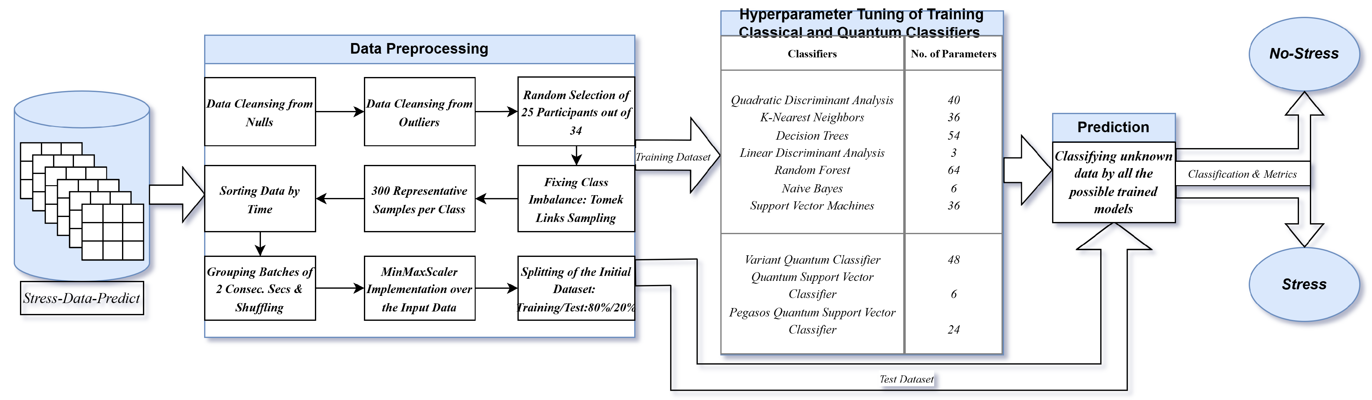
An overview of the complete pipeline, from data collection to the final classification, is provided before examining each component in detail. Figure 1 illustrates the end-to-end methodology that was used for the prediction of stress, depicting the complete transformation sequence from raw data set to the classification output.

Figure 1 details how each stage operates for both classical and quantum computations. For consistency, the same pipeline was implemented for both noisy and noiseless quantum simulations. The process started at the point of gathering the data. The data collection had all of the participant’s individual information, physiological attributes, and the class label for each record.

Data preparation constituted the next stage, comprising nine separate preprocessing steps applied to all classifiers in order to ensure a fair comparison and reliable results. Once the training data had been cleaned up, it was passed to the classification methods. Hyperparameter testing became possible through this particular sequence.

In the testing phase, both the quantum and classical classifiers were evaluated on the held-out data to identify which models produced the highest accuracy and metrics. In total, seven classical and three quantum classifiers were studied; each quantum classifier was evaluated under both noisy and noiseless simulations. Thirteen configurations—seven classical and six quantum (three classifiers × noiseless/noisy)—were compared, yielding the best-performing configurations for this data set. The experimental results reflect the true performance characteristics of the model. These results were compared to help validate additional observations related to how long it took to sort and how accurate the classification was.

3.2. The Data Set

The empirical study was based on a data set created by Iqbal et al. to examine the physiological effects of stress [61]. Since stress produces measurable physiological changes, the Empatica E4 wearable device was utilized to capture these signals. Data related to heart rate and breathing rates were collected during times of stress, as these measures reflect the physiological responses to stress. The Empatica E4 is a research-grade, wrist-worn device incorporating four sensors integrated into it, including a PPG sensor to measure the blood volume pulse in order to determine heart rate; a three-axis accelerometer to measure movement and orientation of the wrist; an electrodermal-activity (EDA) sensor; and an infrared (IR) temperature sensor to measure skin temperature. The two variables that were utilized as predictors for this project were heart rate and respiratory rate. Respiratory rates were determined using the raw PPG waveform [62]. There is an important difference between how ECG data and PPG data are processed. ECG signals are derived from electrodes placed on the chest, provide high temporal resolution, and directly measure the heart’s electrical activity. PPG, on the other hand, indirectly measures both cardiac and respiratory cycles via optical means. It is also more susceptible to artifacts due to movement or perfusion issues at the measurement site. Therefore, this study was specifically designed to assess the low-fidelity, unobtrusive, and consumer-style wearable format as opposed to the high-fidelity ECG format. High-fidelity ECG is the clinical format most relevant to assessing physiological responses to stress continuously in an individual’s daily environment.

Thirty-five healthy participants, ranging in age from 18 to 75 years, volunteered for the research study and wore an Empatica E4. A broad age range was intentionally sought. Women who were breastfeeding and pregnant, as well as color-blind individuals, were excluded from the research, as these characteristics could introduce uncontrolled variability. Color-blind participants were excluded because the Stroop Color–Word Test requires accurate discrimination of the colors; this inability to perform this test invalidates the stress stimulus rather than reflecting the physiological stress response. Similarly, pregnant and breastfeeding women were also excluded in order to avoid introducing uncontrolled variations in autonomic and cardiovascular variability unrelated to the experimentally induced stressors. Each participant signed an informed consent prior to the beginning of the medical measurement collection.

Participants engaged in three different assigned tasks that produced pressure, such as the Stroop Color Test and the Trier Social Stress Test. Resting periods were placed between the assigned tasks since the physical structure required time for physiological recovery. The equipment captured heart rate and breathing rate during task and rest periods. Iqbal et al. reported that respiratory rate can be detected through other signals; therefore, they developed a novel algorithm to estimate respiratory rate from raw PPG signals as described in their work [62]. They employed a Bayesian framework and a time-efficient expectation–maximization (EM) algorithm for the individual-level statistical analysis.

During the Trier Social Stress Test, the largest variations in terms of heart rate and breathing rates were produced. Iqbal et al. reported significant heart rate variations in 27 of the 35 participants (77%) and respiratory rate variations in 28 of the 35 participants (80%). Identifying whether individual participants’ heart rate and respiratory rate deviated from baseline was therefore a critical requirement.

The primary finding revealed that the variations in heart rate and respiratory rate are highly informative for stress detection. Given the discriminative value of the signals, a dedicated data set containing only these two physiological variables was developed to facilitate binary classification for stress detection. This open-access data set makes studying stress monitoring easier when individuals utilize wearable devices like the Empatica E4.

The data set was chosen for its suitability for data preparation and binary classification in this study. This methodology applies binary classification using complex data preparation and optimized classical, quantum and quantum hybrid machine learning algorithms on the data collected by the group of Iqbal et al.

3.3. Data Preprocessing

The Stress-Predict data set was preprocessed to ensure compatibility with both classical and quantum machine learning classifiers, improve data quality, and ensure a fair comparison in the subsequent classification experiments.

Missing data were first addressed by removing all records containing at least one missing value. This reduced the number of cases available for analysis from 112,516 to 112,472. The outliers were identified next based on Tukey’s interquartile range (IQR) method; for each feature, only rows whose values fell within $[Q_1-1.5·\mathrm{IQR},Q_3+1.5·\mathrm{IQR}]$ were retained, where $Q_1$ and $Q_3$ denote the 25th and 75th percentiles, respectively. Based on this process, an additional 3597 cases were dropped. Thus, the clean file contained 108,878 cases. The resulting per-feature IQR values are summarized in

Table 1. Interquartile range (IQR) of features.

Feature	IQR Value
Participant	$1.700000\times {10}^1$
Heart Rate (HR)	$1.569000\times {10}^1$
Respiratory Rate (RR)	$2.685676\times {10}^0$
Time (s)	$1.802372\times {10}^6$
Label	$1.000000\times {10}^0$

.

Rows totaled 3597 fewer once the outlier removal was finished. Twenty-five individuals were selected at random from the entire population of individuals that participated. This sample size was chosen to keep the runtime in the quantum simulation tractable. Both the classical and quantum machine learning classifiers had to be compared in a fair manner; therefore, the same number of individuals was used for both methods.

Class weights were computed from the label distribution to address imbalance; Tomek links undersampling was applied to minimize class overlap, particularly near the decision boundary [63]. This action removed ambiguous data examples so that the success of classification would be enhanced.

Mutual-information-based methods were utilized in the stage of feature selection to identify the most relevant features for each class. Retaining only the most informative features improved computational tractability and classification performance, which is a necessity given that quantum classifiers require medium-sized data sets to operate under the current technological advancements.

Following the feature selection stage, the data sets for each class were decreased to the 300 most representative samples. Reducing the sample size allowed for computations to occur while still maintaining enough variability for training the machine learning models. The data were organized in accordance with the time feature, then grouped into batches that contained two seconds each. These batches were formed to capture time-based patterns, which are essential for machine learning models. To eliminate any potential biases caused by the order of the data, the samples were shuffled after the batching was complete.

To improve the machine learning models, data normalization was applied using MinMaxScaler, which limited all values to be between 0 and 1. StandardScaler normalization was also evaluated but yielded lower accuracy on quantum classifiers; MinMaxScaler was adopted. The data were divided into 80% for the training phase and 20% for the testing phase to finalize the configuration.

Two consequences of this pipeline are acknowledged with full transparency and reviewed in Section 5.6 as well. The first is that the combination of outlier removal, Tomek links cleaning, mutual information feature selection, and per-class subsampling creates a very simple binary problem that can be solved with high accuracy using standard machine learning algorithms. As such, the nearly perfect accuracies reported later may indicate how well each model is able to separate tasks rather than an indication of superior performance on the part of each model. The second result is that the feature set includes time (s), so it appears that in the Stress-Predict protocol, because of the placement of stress and rest blocks at constant time intervals throughout the experiment, the timestamp could potentially serve as a partial proxy for the timing of the block schedule. Both issues are dealt with in detail in Section 5.6 as explicit threats to validity along with those experiments necessary to determine the extent to which they impact the conclusions drawn from the data.

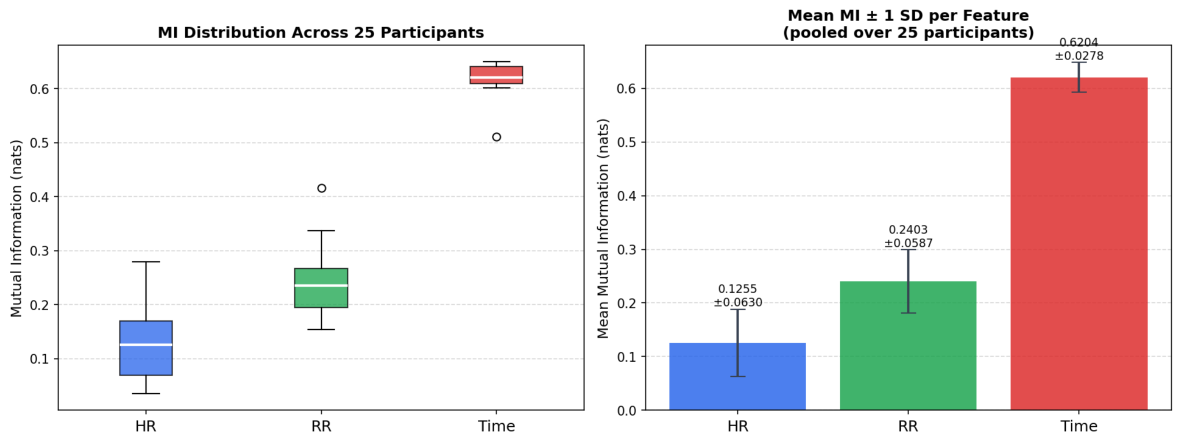
Classical ablation and empirical bounding of the time predictor. Comparing mutual information for each participant reveals that time has the most discriminatory information of the three features examined: $MI\left(Time\right)=0.6204\pm 0.0278$ nats, while $MI\left(RR\right)=0.2403\pm 0.0587$ nats and $MI\left(HR\right)=0.1255\pm 0.0630$ nats (mean ± standard deviation across participants; Figure 2). The results confirm the scheduling-proxy concern. In the Stress-Predict protocol, the fixed temporal positions of the Stroop and Trier stress blocks create an independent temporal gradient from the physiological responses.

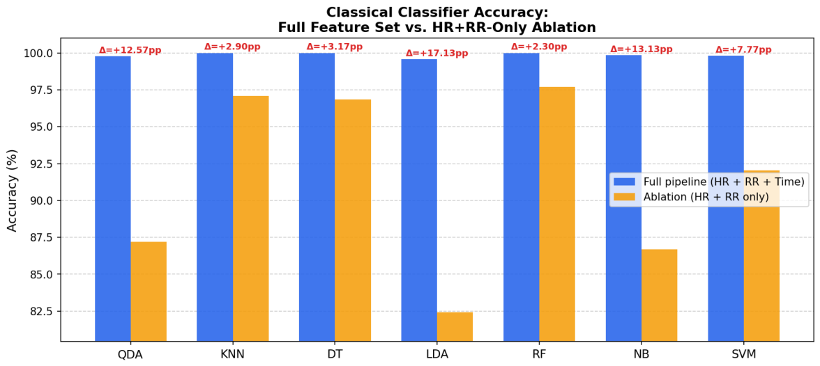
A classical ablation study was conducted to measure each classifier’s dependence on the time feature, using only HR and RR as inputs. All the classifiers were trained using the same preprocessing steps but without using time. The results show that there are two separate behavioral categories. The tree-based or distance-based classifiers—random forest ($\Delta =-2.30$ pp), K-nearest neighbors ($\Delta =-2.90$ pp), and decision trees ($\Delta =-3.17$ pp)—perform well without the time, demonstrating that the physiological separation in HR and RR alone is real. The linear or density-based classifiers—support vector machine ($\Delta =-7.77$ pp), quadratic discriminant analysis ($\Delta =-12.57$ pp), naive Bayes ($\Delta =-13.13$ pp), and linear discriminant analysis ($\Delta =-17.13$ pp)—experience substantially larger drops, indicating that their performance achieved in the original pipeline is due to time’s structural properties and not its physiological content (Figure 3).

These results reinforce the deliberate framing of this study as a noise-aware proof-of-concept benchmark on a physiologically separable data set (Section 2.5). As quantum and classical classifiers used the same set of features throughout this study, the TOST equivalence found in Section 4.5 is consistent within this evaluation context. It remains to be determined whether equivalence will hold in physiology-only data; thus, quantum re-simulation is required and is committed as future work (Section 5.6, item 2).

3.4. The Classical Machine Learning Classifiers

In addition to being able to compare the performance of quantum classifiers with the performance of classical ones, the data set had to undergo preprocessing. The following seven classical machine learning algorithms were evaluated: K-nearest neighbors (KNN); naive Bayes (NB); decision trees (DTs); quadratic discriminant analysis (QDA); linear discriminant analysis (LDA); support vector machines (SVMs); and random forest (RF).

A random search method was used to evaluate many combinations of hyperparameters as listed in

Table 2. Hyperparameters for each classical classifier.

Classifier	Hyperparameter	Values
Quadratic Discriminant Analysis (QDA)	reg_param	{0.00001, 0.0001, 0.001, 0.01, 0.1}
	store_covariance	{True, False}
	tol	{0.0001, 0.001, 0.01, 0.1}
K-Nearest Neighbors (KNN)	n_neighbors	{5, 7, 9, 11, 13, 15}
	weights	{uniform, distance}
	metric	{minkowski, euclidean, manhattan}
Decision Tree (DT)	criterion	{gini, entropy}
	max_depth	range(1, 10, 2)
	min_samples_split	range(1, 10, 2)
	min_samples_leaf	range(1, 5, 2)
Linear Discriminant Analysis (LDA)	solver	{svd, lsqr, eigen}
Random Forest (RF)	n_estimators	{100, 500}
	max_features	{auto, sqrt}
	max_depth	{60, 80}
	min_samples_split	{2, 10}
	min_samples_leaf	{1, 4}
	bootstrap	{True, False}
Naïve Bayes (NB)	priors	{None, [0.5, 0.5]}
	var_smoothing	{$1\times {10}^{-9}$, $1\times {10}^{-6}$, $1\times {10}^{-12}$}
Support Vector Machine (SVM)	C	{0.1, 10, 1000}
	gamma	{1, 0.01, 0.0001}
	kernel	{linear, poly, rbf, sigmoid}

. Additionally, 5-fold cross-validation (CV) was used to evaluate the robustness of each classifier’s performance.

During the training phase, the time it took to build each model was recorded. The best hyperparameter combination for each classifier was determined. The trained models were subsequently applied to generate predictions on the test data set. The time taken to make predictions for the test data set was recorded. The performance of each model was evaluated via a comprehensive classification report, comprising accuracy, precision, recall, and the F1 score. Confusion matrices were also constructed to extract TP, FN, FP, and TN, enabling a granular assessment of classifier quality.

Furthermore, the memory size of each trained model was determined. It provided insight into the computational efficiency of the models. Each classical classifier was therefore evaluated in three ways: classification accuracy, prediction time, and computational efficiency.

3.5. The Quantum Machine Learning Classifiers

In this subsection, the development of the QML classifiers is examined. There are three strategies that can be used to develop QML classifiers. The first strategy, VQC, employs a scalable parameterized circuit architecture for data classification. The second, QSVC, combines classical support vector classification with quantum kernel-based feature mapping. The third, PegasosQSVC [64], is similar to the QSVC but replaces the standard SVM solver with a Pegasos stochastic subgradient descent algorithm. These hybrid quantum classifiers leverage the representational power of quantum circuits and the interpretability of classical optimization.

Therefore, the goal was to identify hyperparameter combinations governing each classifier’s circuit architecture—determining which feature maps, ansatz, and optimizers yield the highest accuracy and associated performance metrics.

Inside the VQC, the main architecture consists of a feature map and an ansatz. The circuit parameters were optimized using gradient-based and gradient-free solvers. Six different feature maps and four different ansatz designs were used with two optimizers. Therefore, there were a total of 48 unique quantum architecture circuits for the target classifiers.

For the QSVC, six different feature maps were evaluated. Therefore, six unique quantum architectures were generated. For the PegasosQSVC, six different feature maps were used and two different regularization parameters (C) were used with two different values for each step size. When the received collection of information was used, 24 cases of PegasosQSVC were studied. These cases are presented in

Table 3. Quantum classifiers and their hyperparameters.

Classifier	Hyperparameter	Values
Variational Quantum Classifier (VQC)	Feature Maps	PauliFeatureMap(num_features, reps=1, alpha=1)
		PauliFeatureMap(num_features, reps=2, alpha=1)
		PauliFeatureMap(num_features, reps=3, alpha=1)
		ZFeatureMap(num_features, reps=1)
		ZFeatureMap(num_features, reps=2)
		ZFeatureMap(num_features, reps=3)
	Ansatzs	RealAmplitudes(num_features, reps=1)
		RealAmplitudes(num_features, reps=2)
		EfficientSU2(num_features, reps=2)
		EfficientSU2(num_features, reps=3)
	Optimizers	SPSA()
		COBYLA()
Quantum Support Vector Classifier (QSVC)	Feature Maps	PauliFeatureMap(num_features, reps=1, alpha=1)
		PauliFeatureMap(num_features, reps=2, alpha=1)
		PauliFeatureMap(num_features, reps=3, alpha=1)
		ZFeatureMap(num_features, reps=1)
		ZFeatureMap(num_features, reps=2)
		ZFeatureMap(num_features, reps=3)
Pegasos Quantum Support Vector Classifier (PegasosQSVC)	Feature Maps	ZFeatureMap(num_features, reps=1)
		ZFeatureMap(num_features, reps=2)
		ZFeatureMap(num_features, reps=3)
		PauliFeatureMap(num_features, reps=1, alpha=1)
		PauliFeatureMap(num_features, reps=2, alpha=1)
		PauliFeatureMap(num_features, reps=3, alpha=1)
	C	[750, 1500]
	Steps	[1000, 1200]

The parameter num_features was set to 3 since, in this case study, the number of features in the data set was three in total: heart rate, respiratory rate, and time. In addition, the feature map function PauliFeatureMap used the single-qubit Pauli gates “Y” and “Z” and the two-qubit Pauli gate “ZZ” for VQC and QSVC models, and the default Pauli gates (“Z” and “ZZ”) for the PegasosQSVC model.

.

As mentioned earlier, the calculated working time for a real quantum computer began with the construction of the classifier. The feature maps and ansatz designs of every classifier were broken down into quantum circuits. These quantum circuits were further broken down into the gate level. By breaking them down, the type and size of gates inside the circuit could be followed. If the gate size was one, the single-qubit gate counter was incremented by one. If the gate size was two, the two-qubit gate counter was incremented by one.

Tau times for single- and two-qubit actions (see Table 3) were multiplied by the total counts of single-qubit and two-qubit gates. The total circuit time for a single shot was obtained by adding the times for both gate types. Calculation for the final running time occurred when the number of shots defined for the simulation was multiplied by the total circuit time for one shot.

The running time of quantum circuits is a critical determinant of the practical feasibility of quantum classifiers. The basic gate operations—single-qubit and two-qubit gates—were analyzed in detail. The total running time was determined by the number of operations and the time that each operation took.

Each quantum circuit (qc) was broken down into its constituent single- and two-qubit gates, and the respective counts were tallied. The specific counters were modified according to the gate type identified during the counting process:

$$\begin{array}{cc}\hfill N_{\mathrm{single}}& =\sum _{\mathrm{gates}\in qc}{⊮}_{\mathrm{single}-\mathrm{qubit}}\left(g\right)\hfill \end{array}$$

(1)

$$\begin{array}{cc}\hfill N_{\mathrm{two}}& =\sum _{\mathrm{gates}\in qc}{⊮}_{\mathrm{two}-\mathrm{qubit}}\left(g\right)\hfill \end{array}$$

(2)

where $⊮$ is the indicator function that assigns 1 when the condition is satisfied.

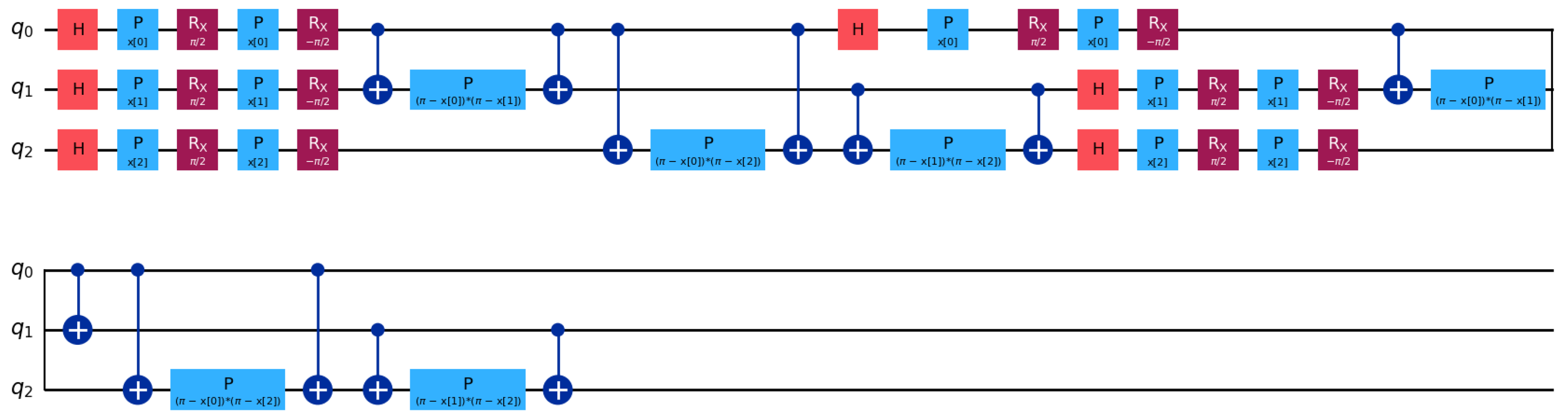
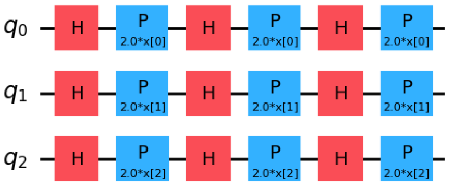
To make Equations (1) and (2) concrete, “breaking down” a circuit means transpiling the feature map and ansatz at a high level of abstraction into the basis of hardware-native gates such that all the operations are either a single-qubit gate (e.g., h, rx, ry, u3, acting on a wire) or a two-qubit entangling gate (e.g., cx, acting on a pair of wires). The counting routine is responsible for the iteration of the decomposed gate list, and an indicator function ${⊮}_{\mathrm{single}-\mathrm{qubit}}\left(g\right)=1$ is evaluated when gate g operates on exactly one qubit, and 0 otherwise. Symmetrically, an indicator function ${⊮}_{\mathrm{two}-\mathrm{qubit}}\left(g\right)=1$ is assessed when gate g operates on exactly two qubits, and 0 otherwise. Therefore, $N_{\mathrm{single}}$ and $N_{\mathrm{two}}$ are simply the number of one- and two-qubit operations in the compiled circuits. These values may be determined directly by inspecting the diagrams of the circuits: in Figure 4, Figure 5 and Figure 6, every H, $R_Y$, $R_Z$, or P block contributes to $N_{\mathrm{single}}$, whereas each pair of vertically connected control–target pairs (denoted by the ⊕ symbol controlling target symbols representing entanglements) contributes to $N_{\mathrm{two}}$. As mentioned above, two-qubit gates also have significantly slower times (${\tau }_{\mathrm{two}}=0.25 \mu \mathrm{s}$ vs. ${\tau }_{\mathrm{single}}=0.05 \mu \mathrm{s}$) than single-qubit gates and are thus also much noisier on real hardware. Consequently, the ratio of two-qubit gates in a given decomposition has been identified as the primary contributor to both the predicted runtime and the noise sensitivity presented later. It follows then that more complex entangled feature maps are expected to degrade more rapidly due to the noise models.

Given the execution time per gate type, denoted as ${\tau }_{\mathrm{single}}$ for single-qubit gates and ${\tau }_{\mathrm{two}}$ for two-qubit gates, the total time needed for gate execution in a quantum classifier is computed as follows:

$$\begin{array}{cc}\hfill T_{\mathrm{single}}& =N_{\mathrm{single}}·{\tau }_{\mathrm{single}}\hfill \end{array}$$

(3)

$$\begin{array}{cc}\hfill T_{\mathrm{two}}& =N_{\mathrm{two}}·{\tau }_{\mathrm{two}}\hfill \end{array}$$

(4)

$$\begin{array}{cc}\hfill T_{\mathrm{total}}& =T_{\mathrm{single}}+T_{\mathrm{two}}\hfill \end{array}$$

(5)

where:

• $T_{\mathrm{single}}$ denotes the total execution time for all single-qubit gates.
• $T_{\mathrm{two}}$ denotes the total execution time for all two-qubit gates.
• $T_{\mathrm{total}}$ is the cumulative execution time for the entire quantum circuit.

This method enables estimation of total circuit execution time and provides a common basis for comparing the computational efficiency of various quantum architectures, simulators, and backends.

Systematic evaluation of different circuit configurations was critical for identifying the most effective quantum classifier architecture. AerSimulator was used in both noise-free and noisy models to evaluate classifier performance under ideal and realistic hardware conditions, respectively. The specific steps for creating a noisy simulation model (that mimics a real quantum computer at extremely high noise levels) is shown in

Table 4. Noise model embedding steps.

Step	Description	Values
1	Initialize parameters: gate times, errors, $T_1$, $T_2$, etc.	${\tau }_{single}=0.05 \mu \mathrm{s}$
		${\tau }_{two}=0.25 \mu \mathrm{s}$
		$erro{r}_{single}=0.01$
		$erro{r}_{two}=0.1$
		$T_1=80 \mu \mathrm{s}$, $T_2=60 \mu \mathrm{s}$
		shots = 256
2	Create noise model instance.	NoiseModel()
3	Add depolarizing errors to gates based on feature map.	For QSVC/PegasosQSVC: h, p, u1, u2, u3, cx
		For VQC: rx, ry, u3
4	Add readout errors to all qubits.	$readou{t}_{error}=0.2$
		ReadoutError matrix:
		$\left[\right[1-0.2,0.2],[0.2,1-0.2\left]\right]$
5	Include amplitude and phase damping errors (for VQC).	Amplitude error: $0.05$
		Phase error: $0.02$
6	Configure noisy backend using AerSimulator.	AerSimulator(method=density_matrix)

. Included in each step are the relevant measurements.

The simulation incorporates the primary contributors to real-world quantum noise through a multi-channel architecture. (i) Stochastic gate failure, represented by depolarization errors on each of the original gate sets, was applied per gate type. Therefore, the total number of failures would increase exponentially for longer circuits. (ii) Measurement (readout) errors; these are modeled via a symmetric bit-flip confusion matrix for errors with a probability of $0.2$ and represent classical assignment errors during measurement. These types of errors were generally the largest error contributors found within current superconducting devices. (iii) Channels representing amplitude and phase damping were used to simulate $T_1$ energy loss and $T_2$ dephasing. Together, the combination of (ii) and (iii) provides qualitative behavior similar to that of a NISQ device rather than a purely stochastic simulator. It is therefore primarily due to the combination of (ii) and (iii) that the degradation of variational circuits (more complex, longer circuits comprising more two-qubit gates) was greater than the degradation observed for the simpler, shallower feature extraction circuit maps.

The noise model is input-signal-independent; it characterizes hardware-level errors in the quantum processor without correlating them to participants’ physiological waveform properties. As mentioned above, this was done intentionally since the noise associated with a processing unit is a characteristic of the hardware itself. Therefore, the authors argue that their results demonstrate tolerance to hardware noise of the quantum processor and not tolerance to variability in physiological signals. Joint modeling of device noise together with subject-specific signal noise is identified as future work in Section 5.6.

3.6. Performance Evaluation Metrics for Classification Models

Several metrics were used to evaluate the performance of classifiers: accuracy, recall, precision, and F1 score. These metrics characterize the effectiveness of each classifier in classifying data precisely between the two classes and were derived from the confusion matrix entries: true positives (TPs), true negatives (TNs), false positives (FPs), and false negatives (FNs).

Accuracy. Accuracy was calculated as the ratio of correctly classified items to the total number of items. The formula for accuracy is:

$$\mathrm{Accuracy}={\displaystyle \frac{TN+TP}{TN+FP+FN+TP}}$$

(6)

Recall. Recall, also known as sensitivity or the true-positive rate, was calculated as the ratio of real positives that the classification models identified correctly. Recall was calculated for each class individually. For example, for class 0 (no-stress) and class 1 (stress),

$${\mathrm{Recall}}_0={\displaystyle \frac{TN}{TN+FP}}$$

(7)

$${\mathrm{Recall}}_1={\displaystyle \frac{TP}{TP+FN}}$$

(8)

High recall values indicate successful identification of positive instances and a low false-negative rate.

Precision. Precision was calculated as the ratio of correctly identified positive items to all items that the classification models identified as positive. High precision is required when false positives incur a large cost. It was calculated for each class after the testing was completed. Precision measures the reliability of the classification models.

$${\mathrm{Precision}}_0={\displaystyle \frac{TN}{TN+FN}}$$

(9)

$${\mathrm{Precision}}_1={\displaystyle \frac{TP}{TP+FP}}$$

(10)

F1 Score. The F1 score is the harmonic mean of precision and recall, providing a single composite measure of classifier performance. This special metric is useful when the two classes are not equally sized. It was recorded for each class because it is essential to have balanced classes. The F1 score is defined as

$$\mathrm{F}1{\mathrm{score}}_0={\displaystyle \frac{2·{\mathrm{Precision}}_0·{\mathrm{Recall}}_0}{{\mathrm{Precision}}_0+{\mathrm{Recall}}_0}}$$

(11)

$$\mathrm{F}1{\mathrm{score}}_1={\displaystyle \frac{2·{\mathrm{Precision}}_1·{\mathrm{Recall}}_1}{{\mathrm{Precision}}_1+{\mathrm{Recall}}_1}}$$

(12)

3.7. Statistical Analysis Methodology

Given the computational cost of quantum circuit simulation, multiple independent test runs were not feasible. Therefore, statistical analysis methods were employed to determine whether differences between classification models were genuine or simply due to random chance. In addition, three complementary methods were adopted: Nadeau–Bengio-corrected cross-validation confidence intervals (CIs), percentile bootstrap CIs, and the two one-sided tests (TOSTs) equivalence test.

3.7.1. Corrected Cross-Validation Confidence Intervals (Classical Classifiers)

When classical classifiers are evaluated with k-fold CV, the standard variance estimator is downwardly biased because the folds are not independent. To correct for this issue, Nadeau–Bengio variance correction [65,66] was used.

Let ${\theta }_j$ denote the performance metric (e.g., accuracy, precision, recall, F1 score, etc.) computed on fold j, where $j=1,\dots ,k$. The average across the k-folds is

$$\overline{\theta }={\displaystyle \frac{1}{k}}{\displaystyle \sum _{j=1}^k}{\theta }_j,$$

(13)

the variance estimate is given by

$$s^2={\displaystyle \frac{1}{k-1}}{\displaystyle \sum _{j=1}^k}{({\theta }_j-\overline{\theta })}^2,$$

(14)

the standard error is defined as

$${\mathrm{SE}}_{\mathrm{std}}={\displaystyle \frac{s}{\sqrt{k}}},$$

(15)

and the corrected standard error is

$${\mathrm{SE}}_{\mathrm{corr}}={\mathrm{SE}}_{\mathrm{std}}\sqrt{1+{\displaystyle \frac{k}{k-1}}}.$$

(16)

The 95% confidence interval (CI) is expressed as

$${\mathrm{CI}}_{95\%}^{\mathrm{corr}}=\overline{\theta }\pm 1.96·{\mathrm{SE}}_{\mathrm{corr}}.$$

(17)

An alternative way of expressing this is as follows. In the canonical Nadeau–Bengio form, we have that ${\mathrm{SE}}_{\mathrm{corr}}^2=\left({\displaystyle \frac{1}{k}}+{\displaystyle \frac{n_{\mathrm{test}}}{n_{\mathrm{train}}}}\right)s^2$, which, for standard k-fold CV, simplifies to Equation (16), using the fact that $n_{\mathrm{test}}/n_{\mathrm{train}}=1/(k-1)$.

Quantifiable measures of statistical uncertainty were provided for each classifier by these CIs. Corrected and bootstrap CIs for classical models are currently the best way to conduct model evaluation under dependent-fold CV. There is theoretical justification for these methods under weak stability conditions, including the hypothesis-testing framework for cross-validated estimators [67,68].

Due to computational constraints, quantum classifiers could each be trained and evaluated only once; Nadeau–Bengio-corrected CV CIs are therefore inapplicable. Instead, uncertainty was quantified using non-parametric percentile bootstrap CIs, enabling statistically meaningful comparisons with classical models despite the asymmetric methodology.

3.7.2. Bootstrap Confidence Intervals (All Classifiers)

To derive non-parametric bootstrap CIs for the performance metric of the classifiers tested in a single test, the percentile method was used [69]. There is widespread convention among researchers that the use of bootstrap CIs is essential when only a single evaluation run is feasible. Bootstrap CIs provide a means to establish a range for the results.

Let ${\widehat{\theta }}^{\left(i\right)}$ denote the performance metric estimated on the i-th bootstrap resample, where $i=1,\dots ,B$, and $B=1000$ iterations. The 95% percentile bootstrap CI is defined as

$${\mathrm{CI}}_{95\%}^{\mathrm{boot}}=\left[Q_{0.025}(\{{\widehat{\theta }}^{(i)}\}),Q_{0.975}(\{{\widehat{\theta }}^{(i)}\})\right],$$

(18)

where $Q_p(·)$ denotes the p-quantile of the empirical bootstrap distribution. This method requires no assumption of normality and is valid near metric boundaries (0 or 1).

3.7.3. Statistical Comparison of Classifiers

The TOST method [70] was used on classifier pairs to test whether their average accuracies were statistically equivalent based on an established margin. In contrast to conventional difference tests, which fail to find significance, TOST offers positive evidence of equivalence by rejecting both one-sided null hypotheses of non-equivalence. The population mean accuracies of classifiers ${\mu }_A$ and ${\mu }_B$ and the equivalency margin ($\Delta >0$) represent how large an absolute difference in mean accuracies would have to exist before it could be reasonably considered as practically insignificant for this problem. Thus, TOST simultaneously tested the two null hypotheses:

$$H_0^{\mathrm{lower}}:{\mu }_A-{\mu }_B\le -\Delta ,H_0^{\mathrm{upper}}:{\mu }_A-{\mu }_B\ge +\Delta .$$

(19)

The two classifiers can be declared to be equal in terms of their statistical performance with a margin of $\Delta$ if both hypothesis tests reject the respective one-sided test. This is equivalent to saying that it can be constructed as a $(1-2\alpha )$ CI and ${\mu }_A-{\mu }_B$ such that it completely contains $[-\Delta ,+\Delta ]$:

$${\mathrm{CI}}_{1-2\alpha }({\mu }_A-{\mu }_B)=\left[({\overline{\theta }}_A-{\overline{\theta }}_B)\pm z_{1-\alpha }·{\mathrm{SE}}_{\mathrm{diff}}\right]\subseteq [-\Delta ,+\Delta ],$$

(20)

where ${\overline{\theta }}_A$ and ${\overline{\theta }}_B$ represent the average accuracy over all k-fold CV estimates for A and B, respectively; $z_{1-\alpha }$ represents the z-score at $1-\alpha$ in a standard normal distribution; ${\mathrm{SE}}_{\mathrm{diff}}$ is the standard error of the difference between two classifiers, computed via propagation from the Nadeau–Bengio-corrected standard error of each classifier individually (assuming independence among folds for different classifiers):

$${\mathrm{SE}}_{\mathrm{diff}}=\sqrt{{\mathrm{SE}}_{\mathrm{corr}}^{{\left(A\right)}^2}+{\mathrm{SE}}_{\mathrm{corr}}^{{\left(B\right)}^2}}.$$

(21)

Throughout the study, $\alpha =0.05$ was used, providing an approximate $90\%$ CI on pairwise accuracy differences. A total of two margins were employed: a strict margin of $\Delta =1$ pp, appropriate for classifiers operating at performance ceilings, and a moderate margin of $\Delta =2$ pp, representing the threshold below which it is improbable to observe clinical distinctions among wearable sensor-based continuous stress monitoring applications with typical variability. Rather than merely stating that there is no statistically significant difference, this method provides affirmative evidence that two classifiers can be practically interchanged.

3.7.4. Summary of Implementation Formulas

Table 5. Formulas used to quantify uncertainty and assess statistical significance for classifier performance.

Method	Formula
Corrected CV SE (classical)	${\mathrm{SE}}_{\mathrm{corr}}={\mathrm{SE}}_{\mathrm{std}}·\sqrt{1+{\displaystyle \frac{k}{k-1}}}$
Standard SE	${\mathrm{SE}}_{\mathrm{std}}={\displaystyle \frac{s}{\sqrt{k}}},s^2={\displaystyle \frac{1}{k-1}}{\sum }_{j=1}^k{({\theta }_j-\overline{\theta })}^2$
Corrected 95% CI	${\mathrm{CI}}_{95\%}^{\mathrm{corr}}=[\overline{\theta }\pm 1.96·{\mathrm{SE}}_{\mathrm{corr}}]$
Bootstrap 95% CI (all)	${\mathrm{CI}}_{95\%}^{\mathrm{boot}}=[Q_{0.025}(\{{\widehat{\theta }}^{(i)}\}),Q_{0.975}(\{{\widehat{\theta }}^{(i)}\})]$
TOST SE of difference	${\mathrm{SE}}_{\mathrm{diff}}=\sqrt{{\mathrm{SE}}_{\mathrm{corr}}^{{\left(A\right)}^2}+{\mathrm{SE}}_{\mathrm{corr}}^{{\left(B\right)}^2}}$
TOST 90% CI of difference	${\mathrm{CI}}_{90\%}({\mu }_A-{\mu }_B)=[({\overline{\theta }}_A-{\overline{\theta }}_B)\pm 1.645·{\mathrm{SE}}_{\mathrm{diff}}]$
TOST equivalence decision	Equivalent at $\Delta$ if ${\mathrm{CI}}_{90\%}({\mu }_A-{\mu }_B)\subseteq [-\Delta ,+\Delta ]$

consolidates all the formulas used in this research to quantify uncertainty and to assess the statistical significance and equivalence of classifierś performance. It collects the corrected cross-validation standard error, the standard error and sample variance, the corrected and bootstrap 95% confidence intervals, and the two one-sided tests (TOST) in order to make the equivalence decisions reported in the next section.

4. Experimental Results

4.1. Cloud Computing Environment and System Specifications

The research was initially conducted in the IBM Quantum Lab Cloud Environment; following its deprecation on 15 May 2024, the QBraid Quantum Environment was adopted. The Pro mode of the QBraid platform was chosen for better performance because the total number of CPUs was eight with 25GB RAM of memory. The AerSimulator was used in both noise-free and noisy configurations to obtain ideal and realistic performance metrics. The libraries used were Qiskit v1.2.0, and Python version 3.11. The experiments were submitted to IBM real quantum computers; however, all jobs failed since the size of the circuits of the classifiers exceeded device capabilities. The simulator was employed throughout with hardware-realistic noise injected to approximate the behavior of real quantum processors.

4.2. The Metrics for the Classical Classifiers

The models of classification were finalized using the optimal hyperparameters determined by 5-fold CV using RandomizedSearchCV. The results of the test data set provided information about the success metrics of each classifier. Because each participant provided a unique data set, the analysis of each data set occurred independently. Statistical measures of performance reflect the specifics of each data set and the average value for each classifier of each participant.

Table 6. Performance and classification metrics of classifiers.

Classifier	Training Time (s)	Prediction Time (s)	Accuracy
DT	$0.1063\pm 0.0196$	$0.0002\pm 0.0001$	$1.0000\pm 0.0000$
KNN	$0.2239\pm 0.0298$	$0.0046\pm 0.0085$	$0.9997\pm 0.0017$
LDA	$0.0522\pm 0.0207$	$0.0002\pm 0.0000$	$0.9937\pm 0.0220$
NB	$0.0295\pm 0.0041$	$0.0002\pm 0.0000$	$0.9967\pm 0.0136$
QDA	$0.1687\pm 0.3611$	$0.0021\pm 0.0090$	$0.9977\pm 0.0088$
RF	$2.4664\pm 0.8678$	$0.0104\pm 0.0071$	$0.9997\pm 0.0017$
SVM	$0.0760\pm 0.0292$	$0.0005\pm 0.0004$	$0.9990\pm 0.0050$

reports training time, prediction time, and accuracy for each classical classifier used in this research. The DT classifier achieved both the fastest training and prediction times and the highest accuracy (100%), making it the most efficient classifier overall. The NB and LDA classifiers had a good trade-off between precision and speed. These classifiers can be used instantly in practical applications.

It should be noted that the RF model required the greatest amount of computation, as it took the longest to train and predict. Despite reaching 99.97% accuracy, RF was not the best choice when fast responses are required. The QDA classifier took varying amounts of time to train. Due to this variability, the computational requirements of the QDA classifier were less predictable than those of the other models. Both the KNN and SVM classifiers achieved high accuracy values of 99.97% and 99.90%. However, due to the longer prediction times of the KNN classifier, the SVM classifier had greater computational efficiency.

All metrics for each classical classifier for both the no-stress and stress classes are listed in

Table 7. Classification metrics per class.

Classifier	No Stress Class			Stress Class
	Recall	Precision	F1 Score	Recall	Precision	F1 Score
DT	$1.0000\pm 0.0000$	$1.0000\pm 0.0000$	$1.0000\pm 0.0000$	$1.0000\pm 0.0000$	$1.0000\pm 0.0000$	$1.0000\pm 0.0000$
KNN	$0.9993\pm 0.0033$	$1.0000\pm 0.0000$	$0.9996\pm 0.0017$	$1.0000\pm 0.0000$	$0.9993\pm 0.0033$	$0.9996\pm 0.0017$
LDA	$0.9987\pm 0.0066$	$0.9899\pm 0.0352$	$0.9943\pm 0.0181$	$0.9888\pm 0.0389$	$0.9985\pm 0.0075$	$0.9936\pm 0.0200$
NB	$0.9953\pm 0.0235$	$0.9988\pm 0.0060$	$0.9970\pm 0.0122$	$0.9985\pm 0.0073$	$0.9947\pm 0.0267$	$0.9966\pm 0.0139$
QDA	$0.9994\pm 0.0032$	$0.9964\pm 0.0133$	$0.9979\pm 0.0069$	$0.9958\pm 0.0155$	$0.9993\pm 0.0037$	$0.9975\pm 0.0080$
RF	$0.9993\pm 0.0034$	$1.0000\pm 0.0000$	$0.9996\pm 0.0017$	$1.0000\pm 0.0000$	$0.9994\pm 0.0032$	$0.9997\pm 0.0016$
SVM	$0.9982\pm 0.0088$	$1.0000\pm 0.0000$	$0.9991\pm 0.0044$	$1.0000\pm 0.0000$	$0.9978\pm 0.0109$	$0.9989\pm 0.0055$

. DT achieved perfect recall, precision, and F1 score across both classes. The KNN classifier followed very closely with an F1 score of 99.96% and almost perfect recall and precision. The NB classifier yielded strong overall results, with a recall of 99.53%, a precision of 99.88%, and an F1 score of 99.70%.

Although the precision of 98.99% was slightly less than the other classifiers for the LDA classifier, the F1 score was still 99.43%. This result indicates a slight increase in the number of false positives when compared to the other classifiers. A nearly complete recall of 99.94%, a precision of 99.64%, and an F1 score of 99.79% were demonstrated by the QDA classifier, indicating that the QDA classifier is excellent at detecting no-stress examples. The RF and SVM classifiers demonstrated a high degree of ability for generalizing, as both had nearly complete performance, with F1 scores of 99.96% and 99.91%, respectively.

Since the stress class was the focus of this study, the DT, RF, and SVM classifiers demonstrated total recall, precision, and F1 scores. The results demonstrate the ability of these classifiers for highly accurate classification of both classes. Although the precision of the KNN classifier was slightly decreased to 99.93%, the F1 score was 99.96% and the recall was perfect. Superior performance was maintained by the NB and QDA classifiers as they had F1 scores of 99.66% and 99.75%, respectively. The LDA classifier was the weakest performer on the stress class, with a notably lower recall of 98.88% and an F1 score of 99.36%, reflecting a higher false-negative rate relative to other classifiers.

4.3. The Best Architectures and the Metrics of the Quantum Classifiers

After exhaustive investigation of all configurations—48 for VQC, 6 for QSVC, and 24 for PegasosQSVC—under both noise-free and noisy conditions, the best-performing architecture for each classifier was identified. The settings that were selected formed the basis for developing the quantum-circuit construction plans that matched each quantum classifier.

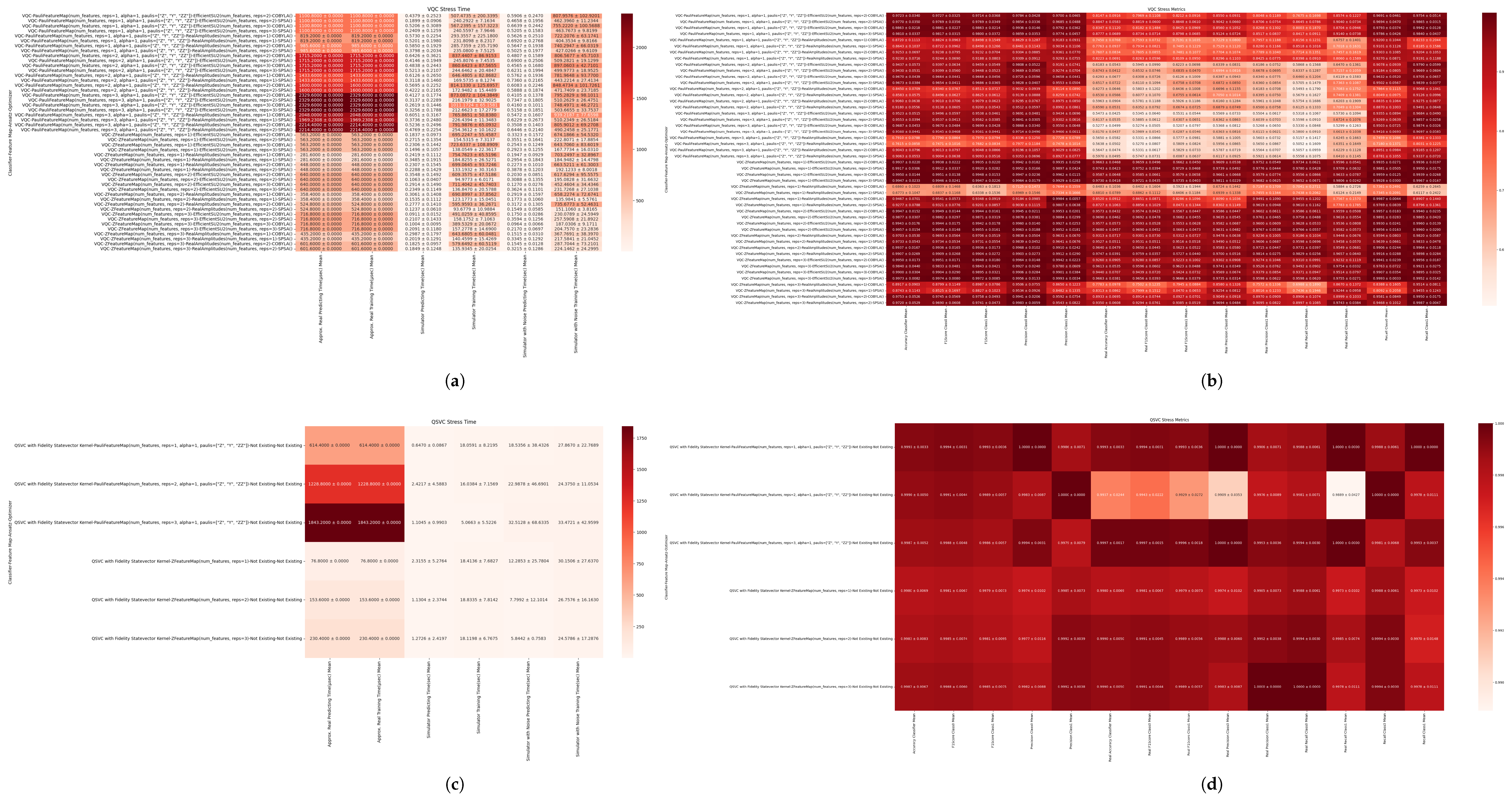
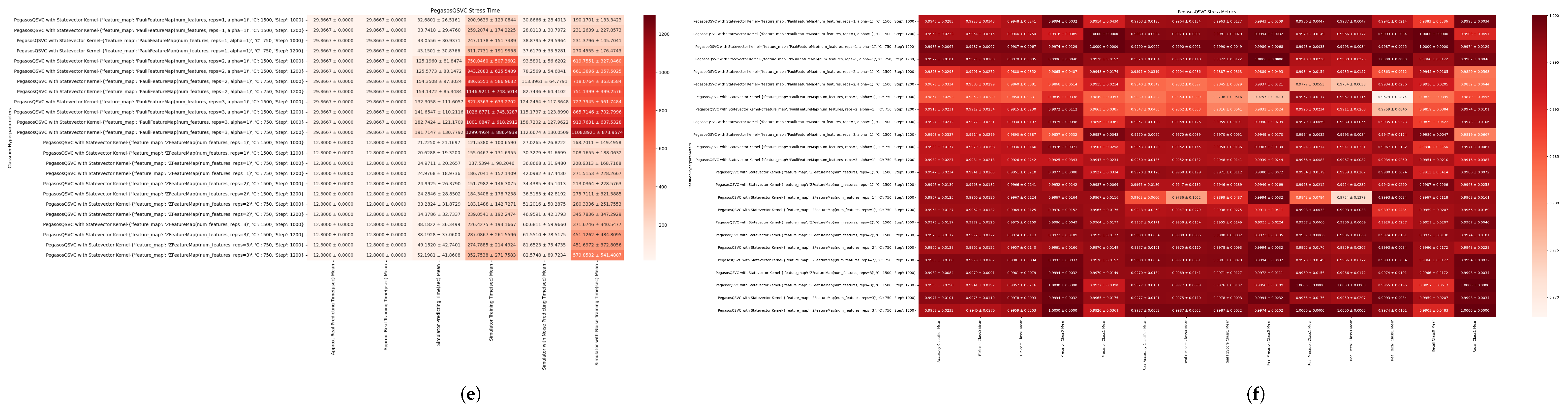
Figure 4, Figure 5 and Figure 6 illustrate how the quantum circuits were developed for the VQC, QSVC, and PegasosQSVC classifiers. In addition, the original circuit structures for the QSVC and PegasosQSVC are also depicted as they function in quantum kernel-based classifiers. Figure 4 displays the final construction plan of the variational quantum classifier (VQC), where the best combination of parameters were determined using the measurement criteria. The heatmap tables of these results are located in the appendix for both noisy and noiseless simulation systems. There is one ZFeatureMap mapping tool and three EfficientSU2 repetitions in this construction plan. For the training phase, the SPSA optimizer was used.

The first figures presenting the initial quantum circuits prior to the application of the mathematical algorithms for the QSVC and PegasosQSVC are Figure 5 and Figure 6. These circuits match the parameters that produced the highest scores and optimal classification measurement criteria. The heatmaps in the appendix illustrate the results for both noiseless and noisy simulation systems. The QSVC employs a PauliFeatureMap with two repetitions, while PegasosQSVC uses a ZFeatureMap with three repetitions.

When testing the VQC, QSVC, PegasosQSVC, and their respective noisy versions, all models demonstrated extremely high performance in all categories. This demonstrates that QML models are efficient regardless of the amount of noise present.

Table 8. Performance and classification metrics of the quantum classifiers.

Quantum Classifier	Training Time (s)	Prediction Time (s)	Accuracy
VQC	$138.0549\pm 22.3617$	$0.1496\pm 0.1057$	$0.9947\pm 0.0233$
VQC Noise	$167.7734\pm 16.0310$	$0.2923\pm 0.1255$	$0.9730\pm 0.0418$
QSVC	$16.0384\pm 7.1569$	$2.4217\pm 4.5883$	$0.9990\pm 0.0050$
QSVC Noise	$24.3750\pm 11.0534$	$22.9878\pm 46.6901$	$0.9937\pm 0.0244$
PegasosQSVC	$226.4275\pm 193.1667$	$38.1822\pm 36.3499$	$0.9980\pm 0.0084$
PegasosQSVC Noise	$371.6746\pm 340.5477$	$60.6811\pm 59.9660$	$0.9970\pm 0.0134$

and

Table 9. Classification metrics per class of the quantum classifiers.

Quantum Classifier	No Stress Class			Stress Class
	Recall	Precision	F1 Score	Recall	Precision	F1 Score
VQC	$0.9928\pm 0.0300$	$0.9964\pm 0.0179$	$0.9946\pm 0.0175$	$0.9947\pm 0.0226$	$0.9967\pm 0.0167$	$0.9957\pm 0.0141$
VQC Noise	$0.9652\pm 0.0671$	$0.9811\pm 0.0229$	$0.9731\pm 0.0359$	$0.9682\pm 0.0625$	$0.9806\pm 0.0242$	$0.9744\pm 0.0338$
QSVC	$0.9983\pm 0.0087$	$0.9991\pm 0.0044$	$0.9987\pm 0.0049$	$0.9989\pm 0.0057$	$1.0000\pm 0.0000$	$0.9994\pm 0.0029$
QSVC Noise	$0.9909\pm 0.0353$	$0.9943\pm 0.0222$	$0.9926\pm 0.0209$	$0.9976\pm 0.0089$	$0.9929\pm 0.0272$	$0.9952\pm 0.0144$
PegasosQSVC	$0.9994\pm 0.0032$	$0.9979\pm 0.0091$	$0.9986\pm 0.0048$	$0.9970\pm 0.0149$	$0.9981\pm 0.0079$	$0.9975\pm 0.0084$
PegasosQSVC Noise	$0.9972\pm 0.0111$	$0.9969\pm 0.0141$	$0.9970\pm 0.0090$	$0.9969\pm 0.0156$	$0.9971\pm 0.0127$	$0.9970\pm 0.0101$

contain all relevant results for every quantum classifier and both groups.

The ideal noiseless classifiers achieved accuracies exceeding 99%, while noisy variants attained at least 97.30%. The QSVC and PegasosQSVC proved resilient, achieving 99.37% and 99.70% accuracies under noise, respectively.

Both the training and prediction procedures were conducted within acceptable time limits for each computational model. Although noise was added to the simulation, this increased the computational time for the PegasosQSVC model. These models can be practically implemented, as their theoretical execution times are relatively short.

High levels of recall, precision, and F1 scores for the “No Stress” and “Stress” classes were achieved by all of the classifiers. Scores for F1 and recall were frequently greater than 99% and rarely varied when the simulation was ideal (noiseless). A high-quality level of classification was maintained when noise was added to the simulation. The F1 score of 99.70% was achieved by PegasosQSVC Noise, demonstrating exceptional noise robustness.

Across both noiseless and noisy conditions, the quantum classifiers achieved high accuracy and stability, demonstrating robust generalization under simulated hardware noise.

4.4. Comparison Between Classical and Quantum Classifiers’ Metrics

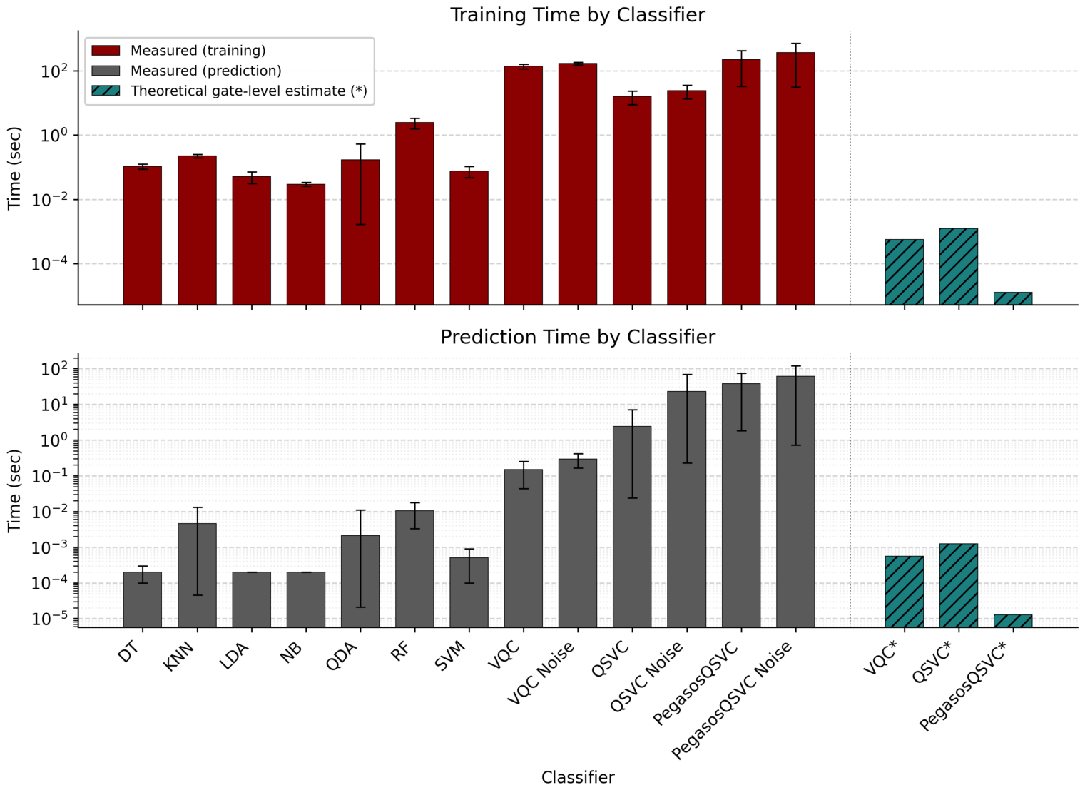
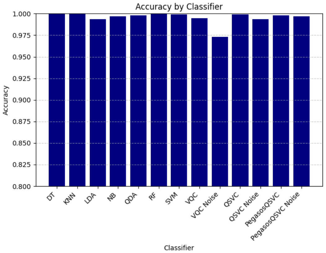
The results from the comparisons of training and prediction times for the classifiers demonstrated in Figure 7 indicated that the classical classifiers were able to finish their work before the quantum classifiers. This is because the quantum classifiers were developed and trained using a quantum simulator, the AerSimulator, which executes on classical hardware.

In addition to requiring one to two orders of magnitude more time to prepare the quantum models than the classical models, there were additional obstacles to overcome by the quantum classifiers due to noise. It is well established that noise-affected quantum classifiers are impractical for real-time applications when simulated on classical hardware. Currently, the simulations of these noisy quantum classifiers are hosted on classical hardware.

Although the current computational requirements of quantum classifiers limit the usefulness of quantum classifiers in applications where rapid results are needed, it is still possible for quantum classifiers to utilize quantum effects in complex data spaces. Quantum classifiers remain less mature than classical models refined over decades. Therefore, progress in quantum hardware, circuit design, and noise reduction must continue until the gap in performance between these technologies is narrowed.

Table 10. Theoretical performance of quantum classifiers. These values represent an analytical lower bound for what has been demonstrated in the experimental results; it is derived from the number of gates compiled to perform both single-qubit and two-qubit operations multiplied by the estimated time to perform each type of operation at ideal conditions (${\tau }_{\mathrm{single}}=0.05 \mu$s, ${\tau }_{\mathrm{two}}=0.25 \mu$s). It assumes that there are no defects, the device has full connectivity so every qubit can interact with any other, there is no transpilation time, there is no delay due to performing readouts of qubits and there is no overhead for error correction. Therefore, these theoretical values are not representative of the current or near-term capability of any existing quantum processor. Instead, they should be viewed strictly as a future-looking benchmark and not as a measure of past or present performance.

Quantum Classifier	Estimated Time ($\mathbf{\mu }$s)
	Training	Prediction
VQC	$563.2000\pm 0.0000$	$563.2000\pm 0.0000$
QSVC	$1228.8000\pm 0.0000$	$1228.8000\pm 0.0000$
PegasosQSVC	$12.8000\pm 0.0000$	$12.8000\pm 0.0000$

contains information regarding the processing times for each of the different classifier architectures. These processing times were calculated using realistic values of a real quantum computer. As it was stated in previous sections, quantum classifiers were able to train at much shorter times (in microseconds) than classical classifiers that required seconds. PegasosQSVC was approximately 5800 times faster during the training phase than NB, which is the fastest classical model. Rapid training can provide an advantage when the need exists for frequent model updates. The prediction times for the quantum classifiers were very close to the prediction times for the classical classifiers. In addition, PegasosQSVC was the fastest among the quantum classifiers.

Three distinct regimes need to be identified to make a direct comparative assessment of the computational overhead of each classifier as well as their corresponding wall-clock times. (1) Wall-Clock Classical Training and Testing Time: A full classical pipeline that was trained and tested in less than 60 min using an 8-core, 25 GB cloud node. (2) Wall-Clock Quantum Simulation Time: State-vector and density-matrix simulations of the quantum classifiers were performed on the same classical computer and took from two to four orders of magnitude longer per configuration than did the classical models. The entire hyperparameter search of all configurations (i.e., 78 different circuit topologies × 5-fold CV × 25 participant data sets) was completed in approximately two to three months of wall-clock time. This is due solely to the exponential increase in computation time associated with simulating quantum state evolution by a classical computer. This is not a limitation imposed by any aspect of actual quantum hardware. (3) Estimated Wall-Clock Times for Theoretical Execution Using Quantum Hardware (Table 10). The estimated time to perform the operations at the gate level for the fastest quantum classifier PegasosQSVC would take $12.8 \mu$s, while it would take as long as $1228.8 \mu$s for the slowest quantum classifier QSVC. Thus, the theoretically predicted speedup of the fast quantum model over the fastest classical model (e.g., approximately $5800\times$ faster for PegasosQSVC training compared to NB) is purely speculative and contingent upon the availability of working quantum hardware. Therefore, it is good to emphasize these distinctions to ensure that no misleading claims about the efficiency of present-day quantum computing systems are made.

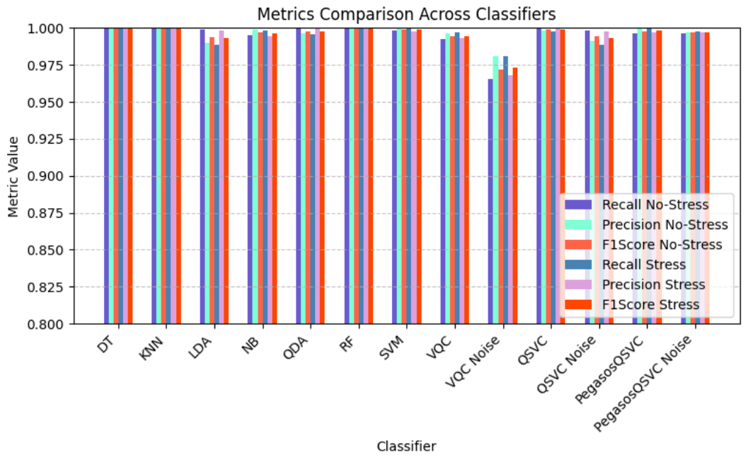
Figure 8 and Figure 9 highlight the results that were obtained by the classical and quantum classifiers when performing tasks related to binary classification. Nearly perfect results were obtained by the classical algorithms. Specifically, the classical algorithms that were included in this evaluation consisted of DT, KNN, LDA, and RF. In addition, the classical algorithms maintained a balance of precision, recall, and F1 score for both classes. Although simulations were conducted without the presence of disturbances, the quantum models (specifically VQC, QSVC, and PegasosQSVC) also obtained excellent results.

It was observed that the quantum classifiers performed robustly in the extreme testing environments that were used to evaluate the limits of modern NISQ hardware. Some of the quantum classifiers did experience slight reductions in performance when disturbances were introduced. PegasosQSVC was able to maintain high accuracy under the same poor environmental conditions as other quantum classifiers. In addition, the high recall and F1 scores of the stress and no-stress classes reflect the robustness of the model, as shown in Figure 9.

When the noise was absent, the VQC achieved high accuracy, but it proved more susceptible to disturbances than PegasosQSVC. By applying hyperparameter tuning to improve the architecture of quantum circuits, it was possible to develop an improved architecture. When the parameters were optimized, the quantum classifiers were able to produce results comparable to the classical models even when the environment had considerable levels of disturbance.

4.5. Statistical Significance and Confidence Interval Analysis

Table 11. 95% Confidence intervals for classifier metrics for classical classifiers. Corrected 95% CIs computed with the Nadeau–Bengio formula ($k=5$, $z=1.96$); bootstrap 95% CIs with $B=1000$ percentile resamples. Both columns are truncated to $[0,1]$.

Classifier	Metric	Estimate	Bootstrap 95% CI	Corrected 95% CI
DT	Accuracy	1.0000	[100.00%, 100.00%]	[100.00%, 100.00%]
	Recall Class0	1.0000	[100.00%, 100.00%]	[100.00%, 100.00%]
	Precision Class0	1.0000	[100.00%, 100.00%]	[100.00%, 100.00%]
	F1 Class0	1.0000	[100.00%, 100.00%]	[100.00%, 100.00%]
	Recall Class1	1.0000	[100.00%, 100.00%]	[100.00%, 100.00%]
	Precision Class1	1.0000	[100.00%, 100.00%]	[100.00%, 100.00%]
	F1 Class1	1.0000	[100.00%, 100.00%]	[100.00%, 100.00%]
KNN	Accuracy	0.9997	[99.83%, 100.00%]	[99.75%, 100.00%]
	Recall Class0	0.9993	[99.67%, 100.00%]	[99.50%, 100.00%]
	Precision Class0	1.0000	[100.00%, 100.00%]	[100.00%, 100.00%]
	F1 Class0	0.9996	[99.82%, 100.00%]	[99.74%, 100.00%]
	Recall Class1	1.0000	[100.00%, 100.00%]	[100.00%, 100.00%]
	Precision Class1	0.9993	[99.67%, 100.00%]	[99.50%, 100.00%]
	F1 Class1	0.9996	[99.82%, 100.00%]	[99.74%, 100.00%]
LDA	Accuracy	0.9937	[97.61%, 100.00%]	[96.48%, 100.00%]
	Recall Class0	0.9987	[99.34%, 100.00%]	[99.00%, 100.00%]
	Precision Class0	0.9899	[96.17%, 100.00%]	[94.36%, 100.00%]
	F1 Class0	0.9943	[97.98%, 100.00%]	[97.05%, 100.00%]
	Recall Class1	0.9888	[95.77%, 100.00%]	[93.77%, 100.00%]
	Precision Class1	0.9985	[99.25%, 100.00%]	[98.86%, 100.00%]
	F1 Class1	0.9936	[97.76%, 100.00%]	[96.73%, 100.00%]
NB	Accuracy	0.9967	[98.58%, 100.00%]	[97.88%, 100.00%]
	Recall Class0	0.9953	[97.65%, 100.00%]	[96.44%, 100.00%]
	Precision Class0	0.9988	[99.40%, 100.00%]	[99.09%, 100.00%]
	F1 Class0	0.9970	[98.72%, 100.00%]	[98.10%, 100.00%]
	Recall Class1	0.9985	[99.27%, 100.00%]	[98.89%, 100.00%]
	Precision Class1	0.9947	[97.33%, 100.00%]	[95.96%, 100.00%]
	F1 Class1	0.9966	[98.55%, 100.00%]	[97.83%, 100.00%]
QDA	Accuracy	0.9977	[99.07%, 100.00%]	[98.61%, 100.00%]
	Recall Class0	0.9994	[99.68%, 100.00%]	[99.52%, 100.00%]
	Precision Class0	0.9964	[98.58%, 100.00%]	[97.89%, 100.00%]
	F1 Class0	0.9979	[99.24%, 100.00%]	[98.88%, 100.00%]
	Recall Class1	0.9958	[98.34%, 100.00%]	[97.54%, 100.00%]
	Precision Class1	0.9993	[99.63%, 100.00%]	[99.44%, 100.00%]
	F1 Class1	0.9975	[99.11%, 100.00%]	[98.70%, 100.00%]
RF	Accuracy	0.9997	[99.83%, 100.00%]	[99.75%, 100.00%]
	Recall Class0	0.9993	[99.66%, 100.00%]	[99.48%, 100.00%]
	Precision Class0	1.0000	[100.00%, 100.00%]	[100.00%, 100.00%]
	F1 Class0	0.9996	[99.82%, 100.00%]	[99.74%, 100.00%]
	Recall Class1	1.0000	[100.00%, 100.00%]	[100.00%, 100.00%]
	Precision Class1	0.9994	[99.68%, 100.00%]	[99.52%, 100.00%]
	F1 Class1	0.9997	[99.84%, 100.00%]	[99.76%, 100.00%]
SVM	Accuracy	0.9990	[99.50%, 100.00%]	[99.24%, 100.00%]
	Recall Class0	0.9982	[99.12%, 100.00%]	[98.66%, 100.00%]
	Precision Class0	1.0000	[100.00%, 100.00%]	[100.00%, 100.00%]
	F1 Class0	0.9991	[99.56%, 100.00%]	[99.33%, 100.00%]
	Recall Class1	1.0000	[100.00%, 100.00%]	[100.00%, 100.00%]
	Precision Class1	0.9978	[98.91%, 100.00%]	[98.35%, 100.00%]
	F1 Class1	0.9989	[99.45%, 100.00%]	[99.17%, 100.00%]

and

Table 12. 95% Confidence intervals for classifier metrics for quantum classifiers. Corrected CV CIs are not applicable (single training run per classifier); bootstrap 95% CIs with $B=1000$ percentile resamples, truncated to $[0,1]$.

Classifier	Metric	Estimate	Bootstrap 95% CI	Corrected 95% CI
VQC	Accuracy	0.9947	[97.61%, 100.00%]	–
	Recall Class0	0.9928	[96.88%, 100.00%]	–
	Precision Class0	0.9964	[98.21%, 100.00%]	–
	F1 Class0	0.9946	[98.06%, 100.00%]	–
	Recall Class1	0.9947	[97.66%, 100.00%]	–
	Precision Class1	0.9967	[98.33%, 100.00%]	–
	F1 Class1	0.9957	[98.44%, 100.00%]	–
VQC Noise	Accuracy	0.9730	[93.96%, 100.00%]	–
	Recall Class0	0.9652	[91.15%, 100.00%]	–
	Precision Class0	0.9811	[96.28%, 99.94%]	–
	F1 Class0	0.9731	[94.44%, 100.00%]	–
	Recall Class1	0.9682	[91.82%, 100.00%]	–
	Precision Class1	0.9806	[96.12%, 100.00%]	–
	F1 Class1	0.9744	[94.74%, 100.00%]	–
QSVC	Accuracy	0.9990	[99.50%, 100.00%]	–
	Recall Class0	0.9983	[99.13%, 100.00%]	–
	Precision Class0	0.9991	[99.56%, 100.00%]	–
	F1 Class0	0.9987	[99.48%, 100.00%]	–
	Recall Class1	0.9989	[99.43%, 100.00%]	–
	Precision Class1	1.0000	[100.00%, 100.00%]	–
	F1 Class1	0.9994	[99.71%, 100.00%]	–
QSVC Noise	Accuracy	0.9937	[97.42%, 100.00%]	–
	Recall Class0	0.9909	[96.27%, 100.00%]	–
	Precision Class0	0.9943	[97.65%, 100.00%]	–
	F1 Class0	0.9926	[97.59%, 100.00%]	–
	Recall Class1	0.9976	[99.05%, 100.00%]	–
	Precision Class1	0.9929	[97.11%, 100.00%]	–
	F1 Class1	0.9952	[98.37%, 100.00%]	–
PegasosQSVC	Accuracy	0.9980	[99.13%, 100.00%]	–
	Recall Class0	0.9994	[99.68%, 100.00%]	–
	Precision Class0	0.9979	[99.06%, 100.00%]	–
	F1 Class0	0.9986	[99.48%, 100.00%]	–
	Recall Class1	0.9970	[98.51%, 100.00%]	–
	Precision Class1	0.9981	[99.18%, 100.00%]	–
	F1 Class1	0.9975	[99.08%, 100.00%]	–
PegasosQSVC Noise	Accuracy	0.9970	[98.63%, 100.00%]	–
	Recall Class0	0.9972	[98.83%, 100.00%]	–
	Precision Class0	0.9969	[98.56%, 100.00%]	–
	F1 Class0	0.9970	[98.98%, 100.00%]	–
	Recall Class1	0.9969	[98.44%, 100.00%]	–
	Precision Class1	0.9971	[98.69%, 100.00%]	–
	F1 Class1	0.9970	[98.89%, 100.00%]	–

present the 95% CIs for performance metrics of classical and quantum classifiers. Percentile bootstrap CIs were computed using B = 1000 bootstrap resamplings for all classifiers. For classical classifiers, the Nadeau–Bengio-corrected CV CIs are provided in addition to bootstrap CIs; the correction accounts for fold dependence and ensures reliable coverage near the upper boundary of the metric scale. Since only one trained model per quantum classifier was possible under budget constraints, corrected CV intervals are not applicable to the quantum classifiers.

The necessity of this warning is justified by our use of the classical standard error, which is based on five quasi-independently generated CV sets using the Nadeau–Bengio adjustment, while the quantum standard error is based solely on a single pass through the test set using a single percentile bootstrapping. It is worth emphasizing that although the classical standard error can be produced independently of each data point in the test set, the bootstrap produces no new realizations of the parameters of the machine learning model itself. Therefore, it cannot represent variability due to the randomness in initializing the model’s weights or optimizing its performance and—critically—shot noise and the stochastic noise associated with the quantum computing channels used; thus, these two estimates have different levels of epistemological assurance even when they are added together as in Equation (21). Because error propagation widens the quantum CIs, making equivalence harder rather than easier to claim, these results, in particular the strict $\Delta =1$ pp QSVC finding, should be regarded as conservative. Therefore, establishing equivalence through symmetric, multiple-run uncertainty quantification will require additional experiments to be performed on physical systems, mentioned in Section 5.6.

TOST equivalence analysis in

Table 13. TOST equivalence test results comparing each quantum classifier against the strongest classical baselines on accuracy, and noise-robustness comparisons within the quantum family. Differences are reported as quantum − classical (or noise-aware − noiseless), in percentage points (pp). A 90% confidence interval on the difference lying entirely within $[-\Delta ,+\Delta ]$ establishes statistical equivalence at margin $\Delta$. The standard error of each difference is obtained by propagation from the Nadeau–Bengio-corrected standard errors under the conservative assumption of fold-level independence across classifiers. Classical classifier SE derives from a 5-fold CV using the Nadeau–Bengio correction; conversely, SE for the quantum classifier derives from a single-run percentile bootstrap variance in the test set that was withheld during quantum classifier training since training multiple versions of our quantum classifier is computational prohibitive. Thus, this difference in methodology can be attributed to current computing resources and, as such, is also conservative in increasing the width of the quantum CIs, thereby making it difficult to establish equivalence rather than easy.

Comparison	Difference (pp)	SE (pp)	90% CI of Difference	Equiv. at $\mathbf{\Delta }\mathbf{=}\mathbf{1}$ pp	Equiv. at $\mathbf{\Delta }\mathbf{=}\mathbf{2}$ pp
Kernel-based quantum (noiseless) vs. strongest classical baselines
QSVC vs. DT	$-0.10$	$0.335$	$[-0.65, +0.45]$	✓	✓
QSVC vs. RF	$-0.07$	$0.354$	$[-0.65, +0.51]$	✓	✓
QSVC vs. SVM	$+0.00$	$0.474$	$[-0.78, +0.78]$	✓	✓
Kernel-based quantum (noise-aware) vs. strongest classical baselines
PegasosQSVC Noise vs. DT	$-0.30$	$0.899$	$[-1.78, +1.18]$	–	✓
PegasosQSVC Noise vs. RF	$-0.27$	$0.906$	$[-1.76, +1.22]$	–	✓
PegasosQSVC Noise vs. KNN	$-0.27$	$0.906$	$[-1.76, +1.22]$	–	✓
PegasosQSVC Noise vs. SVM	$-0.20$	$0.959$	$[-1.78, +1.38]$	–	✓
Variational quantum (noiseless) vs. strongest classical baselines
VQC vs. DT	$-0.53$	$1.563$	$[-3.10, +2.04]$	–	–
VQC vs. RF	$-0.50$	$1.567$	$[-3.08, +2.08]$	–	–
VQC vs. SVM	$-0.43$	$1.599$	$[-3.06, +2.20]$	–	–
Variational quantum (noise-aware) vs. strongest classical baselines
VQC Noise vs. DT	$-2.70$	$2.804$	$[-7.31, +1.91]$	–	–
VQC Noise vs. RF	$-2.67$	$2.806$	$[-7.29, +1.95]$	–	–
VQC Noise vs. SVM	$-2.60$	$2.824$	$[-7.25, +2.05]$	–	–
Noise robustness within the quantum family
PegasosQSVC Noise vs. PegasosQSVC	$-0.10$	$1.061$	$[-1.85, +1.65]$	–	✓
QSVC Noise vs. QSVC	$-0.53$	$1.671$	$[-3.28, +2.22]$	–	–
VQC Noise vs. VQC	$-2.17$	$3.210$	$[-7.45, +3.11]$	–	–

A check mark (✓) indicates statistical equivalence at the corresponding margin $\Delta$ (the 90% CI of the accuracy difference lies entirely within $[-\Delta ,+\Delta ]$ under the TOST procedure). A dash (–) indicates the equivalence criterion was not met.

gives formal statistical evidence that kernel-based quantum classifiers perform similarly to the best classical baselines for the stress detection task; they achieve this under experimental conditions that significantly disadvantage quantum approaches. The QSVC is established as statistically equivalent to DT, RF, and SVM at the strict margin of $\Delta =1$ pp; the pairwise difference CIs span no more than $\pm 0.78$ pp and are centered within $0.10$ pp of zero, the smallest margin at which a meaningful claim of equivalence can be made about highly accurate classifiers. Thus, it precludes the possibility (at $\alpha =0.05$ levels in either direction) that the QSVC and the four leading classical methods differ by up to 1 percent point in their average accuracy. Importantly, this equivalence is valid even though the QSVC was trained using fundamentally different computational paradigms; operates on a quantum feature space of exponential size relative to those accessed through classical kernel methods; and was compared to classical algorithms that have been optimized over the last several decades on this type of signal processing problem.

The significance of these findings is further reinforced by the noise-aware results. When the QSVC and PegasosQSVC were evaluated using a simulated quantum hardware noise model, PegasosQSVC Noise demonstrated equivalence to all four top classical classifiers (DT, RF, KNN, and SVM) at the practically relevant margin of $\Delta =2$ pp. This margin represents an accuracy difference threshold at or below which differences will likely be unimportant for distinguishing clinical stress monitoring outcomes from wearable sensor data. Therefore, the noise-aware quantum classifier demonstrates classical-equivalent accuracy in the environment that is critical for deploying on near-term quantum hardware that cannot avoid decoherence and gate errors. The same TOST framework also establishes PegasosQSVC as being the least sensitive to quantum noise among the studied classifiers. Under simulated noise, PegasosQSVC degrades by only $0.10\%$, while the QSVC degrades by $0.53\%$ and the VQC degrades by $2.17\%$. These results establish Pegasos kernel methods as the most promising candidate for developing hardware-deployed quantum classifiers for stress classification.

In summary, the TOST analysis supports three conclusions that point-estimate comparisons cannot provide. First, the hypothesis that classical baselines consistently outperform kernel-based quantum classifiers on this task is formally rejected at $\alpha =0.05$. Second, while there may exist an advantage to classical methods in terms of raw accuracy (if such an advantage exists), it must be bounded above by $0.78\%$ for the QSVC and by $1.78\%$ for PegasosQSVC Noise—both bounds are far less than the variability inherent in wearable sensors. Finally, the kernel-based quantum approaches (QSVC, PegasosQSVC) not only match classical accuracy but also exhibit a property absent from all classical baselines: demonstration of robustness against quantum hardware noise, which is a necessary condition for large-scale implementation on real quantum processors.

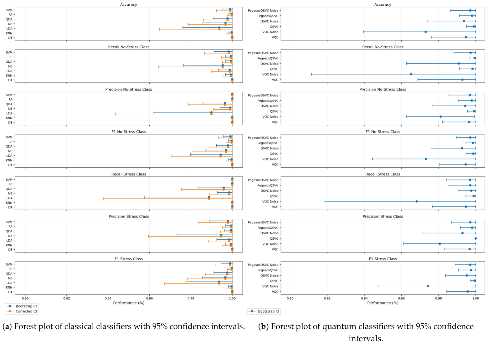
Forest plots showing the performance metrics, along with their 95% CIs for accuracy, precision, recall, and F1 score, can be seen in Figure 10a,b. For example, the VQC, QSVC, and PegasosQSVC were able to achieve point estimates above 0.97 in each metric. Additionally, it appears that the lower bounds of the CIs for these quantum classifiers were also high. Consistently high CI lower bounds reflect the robustness of the optimized quantum classifiers despite the inherent stochasticity of quantum systems.

As the forest plots reveal, quantum classifiers exhibit wider CIs than classical counterparts, particularly for the noise-injected variants, owing to amplified stochastic variability in circuit measurements. Classical classifiers contain narrower CIs and slightly higher point estimates. The reason for this behavior is due to classical classifiers being trained by deterministic processes. In addition, the high degree of separability present in the data allowed the classical classifiers to maintain a consistent and very stable performance. The narrow intervals represent the predictable nature of classical classifiers.

4.6. Comparison with Prior Quantum Stress-Detection Studies

Table 14. Indicative comparison with prior quantum/hybrid stress- and affect-detection studies. Accuracies are as reported by the cited works on their respective data sets and are not directly commensurable due to differing data, tasks, and protocols; the table is intended only to situate the present results within the literature.

Study	Approach/Data Set	Reported Acc.
Padha & Sahoo [9]	VQC/QSVC/QKNN, SWELL and Psykose	∼90%
Padha & Sahoo [41]	QSVC, SWELL-KW (multi-class)	∼80%
Koike-Akino & Wang [42]	Quantum–deep hybrid, EEG stress	87.23–95.12%
Padha & Sahoo [43]	Quantum–LSTM, SWELL-KW and Stress EEG	87.67%
This work (noiseless)	VQC/QSVC/PegasosQSVC, Stress-Predict	99.47–99.90%
This work (NISQ noise)	VQC/QSVC/PegasosQSVC, Stress-Predict	97.30–99.70%

situates these results within the prior QML literature on affect and stress. Prior approaches to QML utilized either pure quantum or hybrid quantum–classical techniques to report classification accuracies generally in the 80–90% range when classifying stress-related data. The noiseless results shown by the optimized QML classifiers surpassed all prior methods, achieving accuracies greater than 99%; under an aggressive NISQ noise model, 97.3% was maintained. Although some portion of this difference can be attributed to the extreme separability inherent in the preprocessed binary version of the task described in Section 5.6, the comparison suggests that selecting features, ansatz, and optimizers systematically and evaluating those selections while aware of potential sources of error produces much more robust behavior from a QML system than that seen in the single-configurations-based evaluations that were prevalent in nearly all prior works.

Finally, since wearable physiological data can be privacy-sensitive, it follows naturally that an interesting and appropriate area for additional investigation would include combining these proposed quantum classifiers with federated learning—in which models are developed on multiple user-distributed computing systems (i.e., the user’s mobile device), yet raw biosignal data from users’ devices are never centrally collected. This could enable collaborative updates to the noise-robust kernel models shown above while keeping patients’ sensitive heart rate and breathing data on the individual’s mobile device; this potential direction is also described as future work in Section 5.6.

5. Discussion

5.1. Key Findings and Comparative Analysis

The classical classifiers—DT, KNN, LDA, and RF—achieved near-perfect performance on both stress and no-stress classes. Quantum models such as the VQC, QSVC, and PegasosQSVC, demonstrated excellent performance in idealized testing environments with no noise. Among the quantum classifiers, PegasosQSVC demonstrated the greatest amount of stability. Although the VQC achieved high accuracy under ideal conditions, it was the most sensitive to noise. This susceptibility is attributable to the deeper variational circuit architecture, which is inherently more vulnerable to NISQ-level decoherence.

All quantum classifiers were evaluated using the Qiskit AerSimulator on classical hardware; physical evaluation was not possible due to the excessive depth of the circuit exceeding available IBM system capabilities. Accordingly, claims regarding noise resistance benefits and projected processing speeds remain speculative pending physical validation.

Computational Expense and Practical Considerations

The simulated evaluation of the quantum classifiers required approximately two to three months of wall-clock time on an 8-core CPU and 25 GB RAM cloud node. In contrast, training and testing the classical models took significantly less time, completing in less than one hour. The large difference in processing time is attributed to the manner in which the state-vector simulation process grows exponentially larger with an increase in the number of qubits. According to experts, the prolonged time did not result from errors in the construction of the quantum architectures [71]. As evidenced by the projected processing times for the circuits, PegasosQSVC may be able to achieve a processing time of as low as $12.8 \mu$s for the prediction phase. A significant portion of the time that it took to complete the project was used to perform a very large search for parameter combinations. The large search consisted of 78 different circuit topologies and 5-fold CV for 25 people.

5.2. Effect of Hyperparameter Optimization

Hyperparameters play a critical role in determining the effectiveness of quantum models. Factors such as feature maps, the depth of the ansatz, the number of circuit iterations, and how the optimizer was selected directly impact the model’s ability to accurately classify in the presence of noise. Optimal hyperparameter selection has been shown here to mitigate the adverse effects of quantum noise.

The “No. of Parameters” for each method depicted in Figure 1 represents the amount of independently adjustable hyperparameters that were evaluated for that specific machine learning model (i.e., 48 different architectural configurations for the VQC compared to 6 for the QSVC or 24 for PegasosQSVC). The “No. of Parameters” is not indicative of how many circuit parameters can be trained. While no monotonic relationship exists between search space size and high accuracy, the QSVC achieved the best noiseless performance due to architectural configuration relative to the VQC; the larger search space for the VQC demanded considerably greater optimization effort. This indicates that while a larger configuration space may reflect more sensitivity to architecture choice and therefore require more efforts to achieve robust results, it is not indicative of whether the results will be improved; as demonstrated in Section 2.5 via feature-map analysis and Appendix A through per-configuration heatmaps.

5.3. Data Attributes and Classical Baselines

Classical classifiers achieved nearly perfect accuracy, with DT achieving 100% and RF achieving 99.97%. This superior accuracy indicates the high intrinsic separability of the preprocessed data set—the result of outlier removal, Tomek links cleaning, mutual information feature selection, and temporal segmentation—leaving minimal scope for quantum models to demonstrate an accuracy advantage. However, the accuracy of the quantum models ranged from 97.30% to 99.90%. The upper limits of these accuracy values represent an improvement over typical results reported in other research studies involving QML [8,60,72].

The implications of this separability are addressed rather than treated as secondary concerns. Since the ability to perform nearly perfect classification using a small number of features (three in this study) and approximately 480 samples allows for a ceiling effect based upon classical methods, it is specifically stated that the scientific contributions from this study will not demonstrate whether QML is required for or performs better than classical machine learning on this specific clinical problem. Instead, the results will be used to provide a controlled comparison (as described in Section 5.6), demonstrating that if one can achieve optimal performance using kernel-based quantum classifiers by systematically searching through architectures, then under a defined NISQ noise model, the classifier can produce statistical results that are identical to those produced by classical classifiers but also have a characteristic that they cannot have: demonstrated measurable robustness to quantum noise.

The classical ablation study, performed in Section 3.3, confirms that tree-based and distance-based classifiers are very robust to the exclusion of time (time has a $\Delta \le 3.2$ pp effect) for RF, DT, and KNN, while linear classifiers have substantial effects (LDA, QDA, NB, SVM), with $\Delta =7.8$–$17.1$ pp. These results indicate that linear classifiers are highly dependent on time as a source of information, and therefore their high classification rates depend on the temporal nature of time and not on the physiological data themselves. In other words, these results confirm the separable testbed hypothesis mentioned previously and provide evidence that there exist HR/RR-based discrimination capabilities independent from the time feature.

Quantum classifiers demonstrated excellent capability in the simulation of noise conditions. The PegasosQSVC achieved a reduction of only 0.10% in the measure of correct classification rates when the system was subjected to depolarizing, readout, and amplitude damping noise. This small reduction confirms that the optimized circuits have a high likelihood of being successfully utilized within NISQ hardware.

5.4. Simulator-Based Evaluation and Hardware Prospects

All experiments were conducted on classical simulators rather than physical NISQ devices, as circuit depths exceeded the capabilities of available hardware. The time available for training did not allow for full variational training, and the vertical path size increased after each step of the hardware-aware transpilation [73,74,75]. Results from the simulators confirm that the algorithmic designs are sound and robust against noise; however, speed and hardware noise robustness must be validated on physical quantum processors before definitive conclusions can be drawn.

Future studies should utilize the new methods of error correction, including zero noise extrapolation and higher quality hardware, to confirm the findings of this study. Time values of $12.8$–$1228.8 \mu$s were calculated for each circuit evaluation and will serve as a benchmark for measuring the increase in speed. Once physical hardware is capable of executing the circuits, the time values will be used as the primary metric for comparisons [76].

Worth mentioning for future work is that the targeted quantum devices, where the quantum classifiers will be evaluated, include superconducting IBM Quantum’s Eagle/Heron family (with 127–156 qubits), whose native error-reduction tools can be accessed via Qiskit Runtime, and the trapped-ion technology utilized at IonQ Forte (where high-quality two-qubit operations and full connectivity allow for the dense entanglement typical of PauliFeatureMap-based QSVCs). Three-qubit sequences employed in this work easily fit within both of these platforms’ resources; it will be qubit utilization (not the number of qubits) that limits the complexity of the quantum circuits once they have been transpiled for hardware (and their depths have been reduced).

5.5. Interpreting Hyperparameter Insights

Heatmaps and circuit visualization revealed clear patterns identifying optimal configurations. The best results for the VQC were achieved when the ZFeatureMap was selected with a single repetition. This particular ZFeatureMap was preferred for its diagonal encoding, limiting cross-feature interference and conferring noise resilience. For the QSVC, the best results were achieved when the PauliFeatureMap was selected with two repetitions. In the case of the QSVC, the ZZ-entanglement was used to establish correlations in physiological features between pairs [77,78,79].

Three repetitions of the EfficientSU2 were employed by the VQC to balance the ability to learn and train. This particular structural approach assisted in avoiding barren plateaus—flat cost-function landscapes induced by noise on NISQ hardware [80,81,82]. For the VQC, SPSA outperformed COBYLA due to its stochastic gradient estimation using perturbations that were relatively insensitive to hardware and shot noise compared to the degradation of COBYLA’s trust region updates with increasing amounts of noise. The use of simultaneous perturbations in SPSA provides a form of implicit stochastic smoothing that is suitable for current levels of noise on NISQ devices [83,84].

For the PegasosQSVC, the best combination included selecting the ZFeatureMap with three repetitions, $C=1500$, and 1200 optimization iterations. Kernel-based methods inherently circumvent barren plateaus by virtue of their non-parametric optimization. Regularization was also selected to clearly separate the groups in the data set.

5.6. Threats to Validity, Limitations, and Future Work

The primary limitations to validity are explicitly enumerated below, along with the associated remediation steps; these limitations are emphasized rather than minimized.

a. Task separability and scope of the claim. Following the data preprocessing pipeline (Tomek links cleaning, outlier elimination, mutual information-based selection of features for classification, and per-class subsampling), the binary classification has become highly separable, as DT achieved 100% and RF achieved 99.97%. Therefore, we do not claim a quantum advantage in terms of clinical or accuracy criteria; instead, the goal of the research is to provide a noise-aware benchmarking and proof-of-concept contribution (Section 3.3 and Section 4.6). The necessary next step, explicitly planned as future work, is to repeat the protocol on a larger and less aggressively curated version of the Stress-Predict data set, also utilizing independent data sets such as WESAD and SWELL-KW, so that quantum and classical behavior can be compared on a genuinely non-trivial decision boundary.

b. Time-feature schedule-proxy risk. The time feature may encode task-scheduling information. A classical ablation study was conducted using only HR and RR as inputs; the methodology and full results are described in Section 3.3 and in Figure 2 and Figure 3. Mutual information analysis confirms that the time feature carries the highest discriminative information of the three features as $MI\left(Time\right)=0.6204\pm 0.0278$ nats versus $0.2403$ for RR and $0.1255$ for HR. An additional finding of the ablation study is that there are two very different types of classifier behaviors: those based on trees or distances (RF $\Delta =-2.30$ pp, KNN $\Delta =-2.9$ pp, DT $\Delta =-3.17$ pp) and those that are linear- or density-based (LDA $\Delta =-17.13$ pp, NB $\Delta =-13.13$ pp, QDA $\Delta =-12.57$ pp, SVM $\Delta =-7.77$ pp); the latter drop much more substantially when the time feature is removed. These findings are reported and reinforce the deliberate proof-of-concept framing established in Section 2.5. Because quantum and classical classifiers were run on the same sets throughout, the results of the statistical tests in Section 4.5 remain internally consistent within the confines of this study’s design. Conducting a full joint classical-plus-quantum ablation, which would require repeating the entire 78-topology hyperparameter search using only the HR and RR, remains as future work due to the multi-month quantum simulation budget. The methodological contributions of this study—the hyperparameter search protocol, NISQ-noise embedding, and TOST equivalence framework—are feature-set invariant and therefore remain valid regardless of the ablation outcome.

c. Quantifying asymmetric uncertainty. Classical classifiers utilize five-fold CV with Nadeau–Bengio correction, while quantum classifiers use a single-run percentile bootstrap (see Section 4.5 for rationale). The error propagation is intentionally conservative, widening the quantum CIs; it does not, however, substitute for independent replicate runs. The equivalence claims—particularly the strict $\Delta =1$ pp QSVC result—are qualified as preliminary throughout the manuscript. Plans include repeating the best kernel models over multiple independent seeds (ultimately on physical hardware) to provide symmetric standard errors.

d. Computational costs associated with simulation vs. prospective benefits related to actual hardware. All results were obtained from simulations on classical computers; thus, the estimated micro-second execution times are based on assumptions regarding hypothetical hardware that currently does not exist at sufficient fidelity (Table 10 caption). Thus, any speed advantages and robustness against noise are speculative projections. The planned target systems for validation and the limited-depth (not qubit-count) nature of true hardware execution are discussed in Section 5.4.

e. Privacy-preserving deployment. Since wearable biosignals are considered to be sensitive, another planned direction includes developing quantum-federated learning models that train noise-robust kernel models across geographically dispersed user-devices without collecting raw heart rate or respiration data centrally (thus matching privacy guidelines for real-world continuous monitoring).

Carefully designed quantum classifiers have the potential to produce results that are similar to those of well-tuned classical models, with noise robustness as a key differentiating strength. The benefit of quantum systems currently is constrained, as classical baselines are able to achieve near-perfect performance; quantum value will most likely materialize as hardware matures. Practical benefits of quantum systems may arise in applications where time is of the essence or when dimensionality is extremely high. This study was completed to show that it is possible to evaluate QML on physiological data and account for noise.

6. Conclusions

This research compares classical and quantum classifiers on a binary stress detection task using physiological data collected with wearable sensors. Three quantum classifier architectures were evaluated under both ideal and noise-aware simulation conditions. In each case, the accuracy of the quantum classifiers was greater than or equal to 97.30%, with the narrowest bootstrap 95% CI lower bound being 93.96% for the most noise-affected model (VQC Noise) and 98.63% for the top-performing noise-aware quantum classifier (PegasosQSVC Noise). The TOST equivalence analysis determined that, under the assessed proof-of-concept conditions, kernel-based quantum classifiers achieved accuracy that was statistically equivalent to the highest-performing baselines (QSVC and PegasosQSVC Noise) at margins of $\Delta =1$ pp and $\Delta =2$ pp, respectively; however, variational methods (VQC, VQC Noise) failed to meet the criteria for equivalence at any margin. Additionally, the kernel-based methods also demonstrated marked noise robustness: PegasosQSVC’s accuracy declined by only 0.10% under simulated hardware noise, compared with 0.53% for the QSVC and 2.17% for the VQC. Overall, the kernel-based QML achieves classical-equivalent accuracy while additionally providing quantifiable hardware noise robustness—a property inherently unavailable in classical classifiers.

The study highlights the substantial computational cost associated with the simulation of quantum circuits, which limited the data set size and the number of feasible independent experimental runs. Specifically, the training and prediction time for the quantum classifiers was two to four orders of magnitude longer than their respective classical counterparts and increased even further when simulated noise was introduced into the process. Although this study provides theoretical evidence that kernel-based quantum classifiers can be used as alternative options to classical methods for detecting stress, it is essential that the best-performing kernel-based models (specifically PegasosQSVC) are deployed onto actual physical quantum processors to confirm the noise tolerance observed here. It would also be beneficial to evaluate how well the current findings generalize across larger and more diverse physiological data sets to determine whether they have practical application.

In conclusion, based on the scope of the proof-of-concept, defined in Section 2.5, a statistical equivalency of the noise-aware kernel-based quantum classifier has been demonstrated in this research with respect to well-tuned classical benchmarks using a deliberately separable wearable testbed. A post hoc classical ablation study indicated that the time feature has most of the discrimination power of the entire feature set ($MI\left(Time\right)=0.6204$ nats versus $MI\left(RR\right)=0.2403$ nats and $MI\left(HR\right)=0.1255$ nats), and linear classifiers depend on this temporal feature. However, tree-based classifiers do not need time features to perform exceptionally (RF: $\Delta =-2.30$ pp, DT: $\Delta =-3.17$ pp), confirming that intrinsic physiological separability exists in the HR and RR alone. Importantly, the resilience of tree-based classifiers under time feature removal does not necessarily mean that quantum classifiers will behave the same way because of the different feature-encoding mechanism structures; the ZFeatureMap encodes each individual physiological feature through diagonal rotation, whereas the PauliFeatureMap introduces pairwise ZZ-entanglement operations among features. These structural differences, when the time feature is removed, could affect both quantum and classical classifiers differently, a nuance noted in Section 2.5, which also motivates the physiology-only quantum re-simulations committed as future work. The results regarding quantum equivalency are restricted to the same context where quantum and classical classifiers were tested using identical input values. Physiology-only quantum performance—using HR and RR without time—will be evaluated in future work (Section 5.6 item 2). Rather than contributing clinically relevant results, the novelty of this work lies in providing a reusable and reproducible protocol for testing the robustness of kernel-based quantum classifiers against noise. Two explicit constraints that limit the generalizability—the time-feature-dependent uncertainty in the TOST equivalence bounds and the scheduling-proxy risk in absolute accuracy—are presented in Section 3.3 and Section 4.5, respectively, and are committed to future investigation.

References

1. Yang, X.; Fang, Y.; Chen, H.; Zhang, T.; Yin, X.; Man, J.; Yang, L.; Lu, M. Global, regional and national burden of anxiety disorders from 1990 to 2019: Results from the Global Burden of Disease Study 2019. Epidemiol. Psychiatr. Sci. 2021, 30, e36. [Google Scholar] [CrossRef] [PubMed]
2. Alonso, J.; Liu, Z.; Evans-Lacko, S.; Sadikova, E.; Sampson, N.; Chatterji, S.; Abdulmalik, J.; Aguilar-Gaxiola, S.; Al-Hamzawi, A.; Andrade, L.H.; et al. Treatment gap for anxiety disorders is global: Results of the World Mental Health Surveys in 21 countries. Depress. Anxiety 2018, 35, 195–208. [Google Scholar] [CrossRef] [PubMed]
3. Institute for Health Metrics and Evaluation. GBD Results Tool, Global Health Data Exchange. Available online: https://vizhub.healthdata.org/gbd-results (accessed on 5 September 2023).
4. World Health Organization. Cardiovascular Diseases (CVDs). Available online: https://www.who.int/news-room/fact-sheets/detail/cardiovascular-diseases-(cvds) (accessed on 11 June 2021).
5. Masri, D.; Jaber, L.; Mashal, R.; Albourini, F.; Alsaoud, M.A.; Al-Tarawneh, A.M.A. The Role of Wearables & Technology in Mental Health: Review. In Proceedings of the 2nd International Conference on Cyber Resilience (ICCR), Dubai, United Arab Emirates, 26–28 February 2024; IEEE: New York, NY, USA, 2024; pp. 1–5. [Google Scholar]
6. Nouman, M.; Khoo, S.Y.; Mahmud, M.A.P.; Kouzani, A.Z. Recent Advances in Contactless Sensing Technologies for Mental Health Monitoring. IEEE Internet Things J. 2022, 9, 274–297. [Google Scholar]
7. Xu, Y.; Yang, J.; Kuang, Z.; Huang, Q.; Huang, W.; Hu, H. Quantum computing enhanced distance-minimizing data-driven computational mechanics. Comput. Methods Appl. Mech. Eng. 2024, 419, 116675. [Google Scholar]
8. Gupta, R.S.; Wood, C.E.; Engstrom, T.; Pole, J.D.; Shrapnel, S. A systematic review of quantum machine learning for digital health. npj Digit. Med. 2025, 8, 237. [Google Scholar] [CrossRef] [PubMed]
9. Padha, A.; Sahoo, A. MAQML: A Meta-Approach to Quantum Machine Learning with Accentuated Sample Variations for Unobtrusive Mental Health Monitoring. Quantum Mach. Intell. 2023, 5, 17. [Google Scholar] [CrossRef]
10. Imran, M.; Aftab, U.; Noreen, A.; Ahmed, M.J.; Asghar, M. Quantum Computing for Healthcare: A Review. Future Internet 2023, 15, 94. [Google Scholar] [CrossRef]
11. Onim, M.S.H.; Humble, T.S.; Thapliyal, H. Emotion Recognition in Older Adults with Quantum Machine Learning and Wearable Sensors. arXiv 2025, arXiv:2507.08175. [Google Scholar]
12. Preskill, J. Quantum Computing in the NISQ era and beyond. Quantum 2018, 2, 79. [Google Scholar] [CrossRef]
13. Kumar, G.; Yadav, S.; Mukherjee, A.; Hassija, V.; Guizani, M. Recent Advances in Quantum Computing for Drug Discovery and Development. IEEE Access 2024, 12, 64491–64509. [Google Scholar] [CrossRef]
14. Sagheer, A.; Zidan, M.; Abdelsamea, M.M. A Novel Autonomous Perceptron Model for Pattern Classification Applications. Entropy 2019, 21, 763. [Google Scholar] [CrossRef] [PubMed]
15. Ding, C.; Bao, T.Y.; Huang, H.L. Quantum-Inspired Support Vector Machine. IEEE Trans. Neural Netw. Learn. Syst. 2022, 33, 7210–7222. [Google Scholar] [CrossRef] [PubMed]
16. Dutt, V.; Chandrasekaran, S.; Daz, V.G. Quantum neural networks for disease treatment identification. Eur. J. Mol. Clin. Med. 2020, 7, 57–67. [Google Scholar]
17. Selvan, R.; Ørting, S.; Dam, E.B. Locally orderless tensor networks for classifying two- and three-dimensional medical images. arXiv 2020, arXiv:2009.12280. [Google Scholar]
18. Li, Y.; Xiao, J.; Chen, Y.; Jiao, L. Evolving deep convolutional neural networks by quantum behaved particle swarm optimization with binary encoding for image classification. Neurocomputing 2019, 362, 156–165. [Google Scholar] [CrossRef]
19. Adhikary, S.; Dangwal, S.; Bhowmik, D. Supervised learning with a quantum classifier using multi-level systems. Quantum Inf. Process. 2020, 19, 89. [Google Scholar] [CrossRef]
20. Benedetti, M.; Garcia-Pintos, D.; Perdomo, O.; Leyton-Ortega, V.; Nam, Y.; Perdomo-Ortiz, A. A generative modeling approach for benchmarking and training shallow quantum circuits. npj Quantum Inf. 2019, 5, 45. [Google Scholar] [CrossRef]
21. Amin, J.; Sharif, M.; Gul, N.; Kadry, S.; Chakraborty, C. Quantum machine learning architecture for COVID-19 classification based on synthetic data generation using conditional adversarial neural network. Cogn. Comput. 2022, 14, 1677–1688. [Google Scholar]
22. Amin, J.; Anjum, M.A.; Gul, N.; Sharif, M. A secure two-qubit quantum model for segmentation and classification of brain tumor using MRI images based on blockchain. Neural Comput. Appl. 2022, 34, 17315–17328. [Google Scholar] [CrossRef]
23. Houssein, E.H.; Abohashima, Z.; Elhoseny, M.; Mohamed, W.M. Hybrid quantum-classical convolutional neural network model for COVID-19 prediction using chest X-ray images. J. Comput. Des. Eng. 2022, 9, 343–363. [Google Scholar] [CrossRef]
24. Moradi, S.; Brandner, C.; Spielvogel, C.; Krajnc, D.; Hillmich, S.; Wille, R.; Drexler, W.; Papp, L. Clinical data classification with noisy intermediate scale quantum computers. Sci. Rep. 2022, 12, 1851. [Google Scholar] [CrossRef] [PubMed]
25. Mishra, A.K.; Gupta, I.K.; Diwan, T.D.; Srivastava, S. Cervical precancerous lesion classification using quantum invasive weed optimization with deep learning on biomedical pap smear images. Expert Syst. 2023, 41, e13308. [Google Scholar] [CrossRef]
26. Konar, D.; Bhattacharyya, S.; Gandhi, T.K.; Panigrahi, B.K.; Jiang, R. 3D Quantum-Inspired Self-Supervised Tensor Network for Volumetric Segmentation of Medical Images. IEEE Trans. Neural Netw. Learn. Syst. 2024, 35, 10312–10325. [Google Scholar] [CrossRef] [PubMed]
27. Chen, Z.; Xue, C.; Chen, S.; Guo, G. VQNet: Library for a Quantum-Classical Hybrid Neural Network. arXiv 2019, arXiv:1901.09133. [Google Scholar]
28. Benlamine, K.; Bennani, Y.; Zaiou, A.; Hibti, M.; Matei, B.; Grozavu, N. Distance Estimation for Quantum Prototypes Based Clustering. In Neural Information Processing (ICONIP 2019); Lecture Notes in Computer Science; Gedeon, T., Wong, K., Lee, M., Eds.; Springer: Cham, Switzerland, 2019; Volume 11955, pp. 522–533. [Google Scholar]
29. Maheshwari, D.; Garcia-Zapirain, B.; Sierra-Soso, D. Machine learning applied to diabetes dataset using Quantum versus Classical computation. In Proceedings of the IEEE International Symposium on Signal Processing and Information Technology (ISSPIT), Louisville, KY, USA, 9–11 December 2020; IEEE: New York, NY, USA, 2020; pp. 1–6. [Google Scholar]
30. Chakraborty, S.; Shaikh, S.H.; Chakrabarti, A.; Ghosh, R. A hybrid quantum feature selection algorithm using a quantum-inspired graph theoretic approach. Appl. Intell. 2020, 50, 1775–1793. [Google Scholar] [CrossRef]
31. Maheshwari, D.; Ullah, U.; Osorio Marulanda, P.; García-Olea, A.; Gonzalez, I.; Merodio, J.; Zapirain, B. Quantum Machine Learning Applied to Electronic Healthcare Records for Ischemic Heart Disease Classification. Hum.-Centric Comput. Inf. Sci. 2023, 13, 17. [Google Scholar] [CrossRef] [PubMed]
32. Ishwarya, I.M.S.; Cherukuri, A.K. Quantum-inspired ensemble approach to multi-attributed and multi-agent decision-making. Appl. Soft Comput. 2021, 106, 107283. [Google Scholar] [CrossRef]
33. Maheshwari, D.; Sierra-Sosa, D.; Garcia-Zapirain, B. Variational Quantum Classifier for Binary Classification: Real vs. Synthetic Dataset. IEEE Access 2022, 10, 3705–3715. [Google Scholar]
34. Gupta, H.; Varshney, H.; Sharma, T.K.; Pachauri, N.; Verma, O.P. Comparative performance analysis of quantum machine learning with deep learning for diabetes prediction. Complex Intell. Syst. 2022, 8, 3073–3087. [Google Scholar]
35. Saini, S.; Khosla, P.; Kaur, M.; Singh, G. Quantum Driven Machine Learning. Int. J. Theor. Phys. 2020, 59, 4013–4024. [Google Scholar] [CrossRef]
36. Yano, H.; Suzuki, Y.; Itoh, K.M.; Raymond, R.; Yamamoto, N. Efficient Discrete Feature Encoding for Variational Quantum Classifier. IEEE Trans. Quantum Eng. 2021, 2, 3103214. [Google Scholar] [CrossRef]
37. Ullah, U.; Jurado, A.G.; Gonzalez, I.D.; Garcia-Zapirain, B. A Fully Connected Quantum Convolutional Neural Network for Classifying Ischemic Cardiopathy. IEEE Access 2022, 10, 134592–134605. [Google Scholar] [CrossRef]
38. Li, Y.; Zhou, R.-G.; Xu, R.; Luo, J.; Jiang, S.-X. A Quantum Mechanics-Based Framework for EEG Signal Feature Extraction and Classification. IEEE Trans. Emerg. Top. Comput. 2022, 10, 211–222. [Google Scholar] [CrossRef]
39. Sridevi, S.; Kanimozhi, T.; Issac, K.; Sudha, M. Quanvolution Neural Network to Recognize Arrhythmia from 2D Scaleogram Features of ECG Signals. In Proceedings of the International Conference on Intelligent Technologies and Innovative Applications in Information and Communication Technology (ICITIIT); IEEE: New York, NY, USA, 2022; pp. 1–5. [Google Scholar]
40. Sameer, M.; Gupta, B. A Novel Hybrid Classical-Quantum Network to Detect Epileptic Seizures. medRxiv 2022. [Google Scholar] [CrossRef]
41. Padha, A.; Sahoo, A. Quantum Enhanced Machine Learning for Unobtrusive Stress Monitoring. In Proceedings of the Fourteenth International Conference on Contemporary Computing; Association for Computing Machinery: New York, NY, USA, 2022. [Google Scholar]
42. Koike-Akino, T.; Wang, Y. quEEGNet: Quantum AI for Biosignal Processing. In Proceedings of the IEEE-EMBS International Conference on Biomedical and Health Informatics (BHI), Ioannina, Greece, 27–30 September 2022; IEEE: New York, NY, USA, 2022; pp. 1–4. [Google Scholar]
43. Padha, A.; Sahoo, A. A Parametrized Quantum LSTM Model for Continuous Stress Monitoring. In Proceedings of the 9th International Conference on Computing for Sustainable Global Development (INDIACom), New Delhi, India, 23–25 March 2022; IEEE: New York, NY, USA, 2022; pp. 261–266. [Google Scholar]
44. Jovanovic, L.; Zivkovic, M.; Bacanin, N.; Bozovic, A.; Bisevac, P.; Antonijevic, M. Metaheuristic optimized electrocardiography time-series anomaly classification with recurrent and long-short term neural networks. Int. J. Hybrid Intell. Syst. 2024, 20, 275–300. [Google Scholar] [CrossRef]
45. Minic, A.; Jovanovic, L.; Bacanin, N.; Stoean, C.; Zivkovic, M.; Spalevic, P.; Petrovic, A.; Dobrojevic, M.; Stoean, R. Applying Recurrent Neural Networks for Anomaly Detection in Electrocardiogram Sensor Data. Sensors 2023, 23, 9878. [Google Scholar] [CrossRef] [PubMed]
46. Bacanin, N.; Stoean, C.; Markovic, D.; Zivkovic, M.; Rashid, T.A.; Chhabra, A.; Sarac, M. Improving performance of extreme learning machine for classification challenges by modified firefly algorithm and validation on medical benchmark datasets. Multimed. Tools Appl. 2024, 83, 76035–76075. [Google Scholar] [CrossRef]
47. Majhi, B.; Kashyap, A.; Mohanty, S.S.; Dash, S.; Mallik, S.; Li, A.; Zhao, Z. An improved method for diagnosis of Parkinson’s disease using deep learning models enhanced with metaheuristic algorithm. BMC Med. Imaging 2024, 24, 156. [Google Scholar] [CrossRef] [PubMed]
48. Zivkovic, M.; Bacanin, N.; Antonijevic, M.; Nikolic, B.; Kvascev, G.; Marjanovic, M.; Savanovic, N. Hybrid CNN and XGBoost Model Tuned by Modified Arithmetic Optimization Algorithm for COVID-19 Early Diagnostics from X-ray Images. Electronics 2022, 11, 3798. [Google Scholar] [CrossRef]
49. Mortensen, J.A.; Mollov, M.E.; Chatterjee, A.; Ghose, D.; Li, F.Y. Multi-Class Stress Detection through Heart Rate Variability: A Deep Neural Network Based Study. IEEE Access 2023, 11, 57470–57480. [Google Scholar] [CrossRef]
50. Abd Al-Alim, M.; Mubarak, R.; Salem, N.M.; Sadek, I. A machine-learning approach for stress detection using wearable sensors in free-living environments. Comput. Biol. Med. 2024, 179, 108918. [Google Scholar] [CrossRef] [PubMed]
51. Fu, W.; Yu, B.; Ji, D.; Zhou, Z.; Li, X.; Wang, R.; Lu, W.; Sun, Y.; Dai, Y. Intelligent fibers and textiles for wearable biosensors. Responsive Mater. 2024, 2, e20240018. [Google Scholar] [CrossRef]
52. Cai, Z.; Ye, K.; Luo, H.; Tang, J.; Yang, G.; Xie, H.; Yang, H.; Xu, K. Textile Hybrid Electronics for Multifunctional Wearable Integrated Systems. Research 2025, 8, 0779. [Google Scholar] [CrossRef] [PubMed]
53. Li, C.; Wang, T.; Zhou, S.; Sun, Y.; Xu, Z.; Xu, S.; Shu, S.; Zhao, Y.; Jiang, B.; Xie, S.; et al. Deep Learning Model Coupling Wearable Bioelectric and Mechanical Sensors for Refined Muscle Strength Assessment. Research 2024, 7, 0366. [Google Scholar] [CrossRef] [PubMed]
54. Schmidt, P.; Reiss, A.; Duerichen, R.; Marberger, C.; Van Laerhoven, K. Introducing WESAD, a Multimodal Dataset for Wearable Stress and Affect Detection. In Proceedings of the 20th ACM International Conference on Multimodal Interaction (ICMI ’18), Boulder, CO, USA, 16–20 October 2018; Association for Computing Machinery: New York, NY, USA, 2018; pp. 400–408. [Google Scholar] [CrossRef]
55. Bolpagni, M.; Pardini, S.; Dianti, M.; Gabrielli, S. Personalized Stress Detection Using Biosignals from Wearables: A Scoping Review. Sensors 2024, 24, 3221. [Google Scholar] [CrossRef] [PubMed]
56. Tsai, Y.-Y.; Chen, Y.-J.; Lin, Y.-F.; Hsiao, F.-C.; Hsu, C.-H.; Liao, L.-D. Photoplethysmography-based HRV analysis and machine learning for real-time stress quantification in mental health applications. APL Bioeng. 2025, 9, 026103. [Google Scholar] [CrossRef] [PubMed]
57. Moser, M.K.; Ehrhart, M.; Resch, B. An Explainable Deep Learning Approach for Stress Detection in Wearable Sensor Measurements. Sensors 2024, 24, 5085. [Google Scholar] [CrossRef] [PubMed]
58. Rashid, N.; Mortlock, T.; Al Faruque, M.A. Stress Detection Using Context-Aware Sensor Fusion from Wearable Devices. IEEE Internet Things J. 2023, 10, 14114–14127. [Google Scholar] [CrossRef]
59. Smets, E.; Rios Velazquez, E.; Schiavone, G.; Chakroun, I.; D’Hondt, E.; De Raedt, W.; Cornelis, J.; Janssens, O.; Van Hoecke, S.; Claes, S.; et al. Large-scale wearable data reveal digital phenotypes for daily-life stress detection. npj Digit. Med. 2018, 1, 67. [Google Scholar] [CrossRef] [PubMed]
60. Ozpolat, Z.; Karabatak, M. Performance Evaluation of Quantum-Based Machine Learning Algorithms for Cardiac Arrhythmia Classification. Diagnostics 2023, 13, 1099. [Google Scholar] [CrossRef] [PubMed]
61. Iqbal, T.; Simpkin, A.J.; Roshan, D.; Glynn, N.; Killilea, J.; Walsh, J.; Molloy, G.; Ganly, S.; Ryman, H.; Coen, E.; et al. Stress Monitoring Using Wearable Sensors: A Pilot Study and Stress-Predict Dataset. Sensors 2022, 22, 8135. [Google Scholar] [CrossRef] [PubMed]
62. Iqbal, T.; Elahi, A.; Ganly, S.; Wijns, W.; Shahzad, A. Photoplethysmography-Based Respiratory Rate Estimation Algorithm for Health Monitoring Applications. J. Med. Biol. Eng. 2022, 42, 242–252. [Google Scholar] [CrossRef] [PubMed]
63. Tomek, I. Two Modifications of CNN. IEEE Trans. Syst. Man Cybern. 1976, SMC-6, 769–772. [Google Scholar] [CrossRef]
64. Shalev-Shwartz, S.; Singer, Y.; Srebro, N.; Cotter, A.A. Pegasos: Primal Estimated sub-GrAdient SOlver for SVM. Math. Program. 2011, 127, 3–30. [Google Scholar]
65. Nadeau, C.; Bengio, Y. Inference for the Generalization Error. Mach. Learn. 2003, 52, 239–281. [Google Scholar] [CrossRef]
66. Bouckaert, R.R.; Frank, E. Evaluating the Replicability of Significance Tests for Comparing Learning Algorithms. In Proceedings of the Pacific-Asia Conference on Knowledge Discovery and Data Mining (PAKDD); Springer: Berlin/Heidelberg, Germany, 2004; pp. 3–12. [Google Scholar]
67. Grandvalet, Y.; Bengio, Y. Hypothesis Testing for Cross-Validation; Technical Report; Université de Montréal: Montreal, QC, Canada, 2004. [Google Scholar]
68. Bayle, P.; Bayle, A.; Janson, L.; Mackey, L. Cross-Validation Confidence Intervals for Test Error. In Proceedings of the Advances in Neural Information Processing Systems (NeurIPS), Virtual, 6–12 December 2020. [Google Scholar]
69. Efron, B. Bootstrap Methods: Another Look at the Jackknife. In Breakthroughs in Statistics; Springer: New York, NY, USA, 1979; pp. 569–593. [Google Scholar]
70. Schuirmann, D.J. A Comparison of the Two One-Sided Tests Procedure and the Power Approach for Assessing the Equivalence of Average Bioavailability. J. Pharmacokinet. Biopharm. 1987, 15, 657–680. [Google Scholar] [CrossRef] [PubMed]
71. Arute, F.; Arya, K.; Babbush, R.; Bacon, D.; Bardin, J.C.; Barends, R.; Biswas, R.; Boixo, S.; Brandao, F.G.; Buell, D.A.; et al. Quantum supremacy using a programmable superconducting processor. Nature 2019, 574, 505–510. [Google Scholar] [CrossRef] [PubMed]
72. IBM Quantum. IBM Quantum Challenge Fall 2021: Challenge 3—Quantum Machine Learning, GitHub Repository. 2021. Available online: https://github.com/qiskit-community/ibm-quantum-challenge-fall-2021 (accessed on 30 May 2026).
73. Liu, Y.; Otten, M.; Bassirianjahromi, R.; Jiang, L.; Fefferman, B. Benchmarking near-term quantum computers via random circuit sampling. arXiv 2022, arXiv:2105.05232v2. [Google Scholar]
74. IBM Quantum. Maximum Execution Time for Qiskit Runtime Workloads. IBM Quantum Documentation. 2024. Available online: https://docs.quantum.ibm.com/guides/max-execution-time (accessed on 30 May 2026).
75. Li, G.; Ding, Y.; Xie, Y. Tackling the Qubit Mapping Problem for NISQ-Era Quantum Devices. In Proceedings of the ACM International Conference on Architectural Support for Programming Languages and Operating Systems (ASPLOS); Association for Computing Machinery: New York, NY, USA, 2019; pp. 1001–1014. [Google Scholar]
76. Temme, K.; Bravyi, S.; Gambetta, J.M. Error Mitigation for Short-Depth Quantum Circuits. Phys. Rev. Lett. 2017, 119, 180509. [Google Scholar] [CrossRef] [PubMed]
77. Havlíček, V.; Córcoles, A.D.; Temme, K.; Harrow, A.W.; Kandala, A.; Chow, J.M.; Gambetta, J.M. Supervised learning with quantum-enhanced feature spaces. Nature 2019, 567, 209–212. [Google Scholar] [CrossRef] [PubMed]
78. Singh, K.; Pokhrel, P. Modeling Feature Maps for Quantum Machine Learning. arXiv 2025, arXiv:2501.08205. [Google Scholar]
79. Shaffer, F.; Ginsberg, J.P. An Overview of Heart Rate Variability Metrics and Norms. Front. Public Health 2017, 5, 258. [Google Scholar] [CrossRef] [PubMed]
80. Wang, S.; Fontana, E.; Cerezo, K.; Sharma, K.; Sone, A.; Cincio, L.; Coles, P.J. Noise-induced barren plateaus in variational quantum algorithms. Nat. Commun. 2021, 12, 1. [Google Scholar] [CrossRef] [PubMed]
81. Kandala, A.; Mezzacapo, A.; Temme, K.; Takita, M.; Brink, M.; Chow, J.M.; Gambetta, J.M. Hardware-efficient variational quantum eigensolver for small molecules and quantum magnets. Nature 2017, 549, 242–246. [Google Scholar] [CrossRef] [PubMed]
82. Cerezo, M.; Sone, A.; Volkoff, T.; Cincio, L.; Coles, P.J. Cost function dependent barren plateaus in shallow parametrized quantum circuits. Nat. Commun. 2021, 12, 1791. [Google Scholar] [CrossRef] [PubMed]
83. Spall, J.C. Implementation of the simultaneous perturbation algorithm for stochastic optimization. IEEE Trans. Aerosp. Electron. Syst. 1998, 34, 817–823. [Google Scholar] [CrossRef] [PubMed]
84. Singh, H.; Majumder, S.; Mishra, S. Benchmarking of different optimizers in the variational quantum algorithms for applications in quantum chemistry. J. Chem. Phys. 2023, 159, 044117. [Google Scholar] [CrossRef] [PubMed]
Figure 1. The end-to-end architecture schema—all necessary steps from data set to classification for classical, quantum, and quantum-with-noise classifiers. (Created in diagrams.net (https://app.diagrams.net/) application.)
Applsci 16 06132 g001
Figure 2. Mutual information between each feature and the stress label, computed across all 25 participants using mutual_info_classif on the raw (pre-Tomek, pre-subsampling) data. (Left): distribution of mutual information values per participant shown as boxplots, where the white line marks the median, the box spans the interquartile range (Q1–Q3), the whiskers extend to 1.5   × IQR, and open circles denote per-participant outliers beyond that range. (Right): pooled mean ± 1 SD across participants. Time yields substantially higher mutual information ( 0.6204 ± 0.0278 nats) than the physiological signals HR ( 0.1255 ± 0.0630 nats) and RR ( 0.2403 ± 0.0587 nats), confirming the schedule-proxy role of the temporal feature in the Stress-Predict protocol. Tree-based classifiers that remain robust under ablation (RF, DT, KNN; see Figure 3) are those whose non-linear decision boundaries exploit the physiological clusters in HR and RR rather than the linear temporal gradient.
Applsci 16 06132 g002
Figure 3. Classical classifier accuracy under the full feature set (HR, RR, time; blue) versus the HR+RR-only ablation (orange). Annotated Δ values denote the accuracy drop in percentage points when time is excluded. Two distinct behavioural groups are evident: tree-based and distance-based classifiers—RF ( Δ = 2.30 pp), KNN ( Δ = 2.90 pp), and DT ( Δ = 3.17 pp)—remain robust on physiological features alone, confirming genuine HR/RR separability; linear and density-based classifiers—SVM ( Δ = 7.77 pp), QDA ( Δ = 12.57 pp), NB ( Δ = 13.13 pp), and LDA ( Δ = 17.13 pp)—experience substantially larger drops, indicating dependence on time’s temporal gradient. All classifiers were trained with the identical preprocessing pipeline, hyperparameter grid, and 5-fold RandomizedSearchCV as in the main experiments; the only variable changed is the exclusion of the time feature.
Applsci 16 06132 g003
Figure 4. The final architecture schema of the variational quantum circuit. The gate boxes are colored automatically by Qiskit according to gate type (the gate name is also printed in each box, so color carries no additional information): H the Hadamard gate, P a phase gate, and R X / R Y / R Z single-qubit rotations. A filled dot (•) joined by a vertical line to ⊕ denotes a CNOT (controlled-X) gate, with • the control and ⊕ the target. In the gate labels, “∗” denotes multiplication, x [ i ] the i-th input feature, and θ [ k ] a trainable circuit parameter.
Applsci 16 06132 g004
Figure 5. The final quantum circuit before the implementation of the QSVC algorithm. The gate boxes are colored automatically by Qiskit according to gate type (the gate name is also printed in each box, so color carries no additional information): H the Hadamard gate, P a phase gate, and R X / R Y / R Z single-qubit rotations. A filled dot (•) joined by a vertical line to ⊕ denotes a CNOT (controlled-X) gate, with • the control and ⊕ the target. In the gate labels, “∗” denotes multiplication and x [ i ] the i-th input feature; this data-encoding circuit contains no trainable parameters.
Applsci 16 06132 g005
Figure 6. The final quantum circuit before the implementation of the PegasosQSVC algorithm. The gate boxes are colored automatically by Qiskit according to gate type (the gate name is also printed in each box, so color carries no additional information): H the Hadamard gate, P a phase gate, and R X / R Y / R Z single-qubit rotations. A filled dot (•) joined by a vertical line to ⊕ denotes a CNOT (controlled-X) gate, with • the control and ⊕ the target. In the gate labels, “∗” denotes multiplication and x [ i ] the i-th input feature; this data-encoding circuit contains no trainable parameters.
Applsci 16 06132 g006
Figure 7. Timing data for training and prediction for each of the classical and quantum models on the simulator and estimated performance for the quantum model on an actual quantum computer. Time is plotted on a base-10 logarithmic scale, as this allows for a comparison of the large orders of magnitude difference in classical vs. quantum simulated time among all models. Bars show ± 1 sample SD across 5-fold CVs; if an SD was greater than the mean (lower whisker would be negative), lower whiskers were trimmed at 99 % of bar height for display purposes only—Table 6 and Table 8 show the true values. The last three teal hatch bars (VQC*, QSVC*, PegasosQSVC*) are the theoretical and computed gate-level time estimates given in Table 10, converted from μ s to seconds; these are based on completely idealized, defect-free, highly connected hardware with no overhead due to transpilation, readout, or error mitigation and cannot currently be achieved by any quantum processor. An asterisk (*) marks these idealized gate-level estimates on theoretical fault-free quantum hardware. The vertical dotted separators in the figure delimit the classical, simulated-quantum, and theoretical-hardware groupings and carry no quantitative value.
Applsci 16 06132 g007
Figure 8. All the classical and quantum classifiers’ accuracy.
Applsci 16 06132 g008
Figure 9. All the classical and quantum classifiers’ metrics.
Applsci 16 06132 g009
Figure 10. Forest plots showing 95% confidence intervals for classical (a) and quantum (b) classifiers.
Applsci 16 06132 g010