Article

A Semi-Analytical Method for a Fast Estimation of the Magnetostatic Forces Acting on Tokamak Components


by
Gennaro Di Mambro
1,2,
Andrea Gaetano Chiariello
2,3,*,
Antonio Maffucci
1,2,
Salvatore Ventre
1,2,
Domenico Marzullo
4,
Enrico Occhiuto
4,
Basilio Esposito
5 and
Daniele Marocco
5
1
Department of Electrical and Information Engineering “M. Scarano”, University of Cassino and Southern Lazio, 03043 Cassino, FR, Italy
2
C.R.E.A.T.E. Research Consortium, 80125 Naples, Italy
3
Department of Engineering, University of Campania “Luigi Vanvitelli”, 81031 Aversa, CE, Italy
4
Department of Engineering and Architecture, University of Trieste, Piazzale Europa 1, 34127 Trieste, Italy
5
Nuclear Department, ENEA, C.R. Frascati, Via E. Fermi 45, 00044 Frascati, RM, Italy
*
Author to whom correspondence should be addressed.
Appl. Sci. 2026, 16(12), 6099; https://doi.org/10.3390/app16126099
Submission received: 5 May 2026 / Revised: 10 June 2026 / Accepted: 12 June 2026 / Published: 16 June 2026

Abstract

High-intensity magnetic fields in tokamak structures for nuclear fusion generate significant ferromagnetic forces that must be properly estimated for a reliable design of the mechanical structures. Accurate numerical modeling of these electromagnetic problems is likely to entail high computational costs due to the complexity of the geometries and the need to account for nonlinear material behavior. However, electromagnetic forces are not the only loads acting on tokamaks, as other phenomena, such as seismic forces, must also be considered in their design. Therefore, it is highly beneficial to develop coarse estimates of the electromagnetic loads in order to compare their magnitude with that of other loads. Such estimates are useful not only in the early stages of design, but also in the final design phase, particularly if these forces prove to be negligible. To this end, this paper proposes a semi-analytical method to quickly estimate the forces acting on ferromagnetic components located outside the vessel. The method is based on the calculation of the magnetization by means of a well-established integral method after a coarse discretization of the volume occupied by the ferromagnetic materials. The proposed method is implemented in computational routines made available within this paper, enabling the estimation of these forces even for users who lack the expertise required to operate commercial simulation tools. The method is applied to case studies related to some export components of the ITER tokamak, and the validation is carried out with reference to the accurate numerical solutions provided by both commercial and in-house simulation tools.

1. Introduction

Nuclear fusion is recognized as one of the most promising options for sustainable energy generation. One of the central devices in this field is the Tokamak [1], which confines high-temperature plasma through magnetic coil systems regulated by advanced control mechanisms. Fusion reactions within the plasma—such as the fusion of two hydrogen nuclei—convert the resulting mass defect into extractable energy [2].
Existing tokamaks, including EAST, JET, KSTAR, JT-60SA, and WEST, or tokamaks under construction or design (e.g., ITER or EU-DEMO), have provided essential platforms for investigating magnetic confinement and advanced plasma scenarios [3,4,5,6,7]. In such extreme environments, the accurate identification of the mechanical loads (forces and torques) acting on components is critical. For systems governed by magnetohydrodynamics (MHD [8]), a precise definition of these loads underpins safe and consistent design.
Complementary research efforts address these challenges from multiple perspectives. Three-dimensional neutronic analyses of tokamak designs have delivered high-resolution data on nuclear heating, neutron damage, and helium production, essential for material selection [9]. Other works focus on the thermal–hydraulic performance of the DEMO divertor cassette body (CB) [10] or on mock-ups supported by CAD modeling with thermal–hydraulic and structural validation [11]. Further studies highlight critical issues such as neutron damage thresholds and localized hot spots, with corresponding design solutions [12].
Moreover, Mazzone et al. [13] investigated the structural performance of ITER components under seismic events, accounting for dynamic interaction between tokamak structures, surrounding buildings, and soil. Linear dynamic approaches, such as power spectral density (PSD) and spectral analysis, provided support loads, accelerations, and relative displacements crucial for seismic design.
Beyond thermal, structural, neutronic, and seismic aspects, electromagnetic loads are equally significant due to the extremely strong magnetic fields of tokamaks. These loads arise mainly from field interactions with induced eddy currents during transient events (e.g., disruptions) and from magnetization of ferromagnetic structural materials [14]. For instance, a vertical displacement event (VDE) can induce large Lorentz forces through plasma–field coupling [15]. In tokamaks like ITER and EU-DEMO, the interaction of strong magnetic fields—about 8T in EU-DEMO [16] and up to 11T in ITER [17]—with ferromagnetic construction materials generates substantial electromagnetic forces. As shown in [18], the contribution of preload in the form of ferromagnetic stress is of particular importance. Similar issues arise in electrical machines [19], where magnetization significantly affects forces and torques. Moreover, the quantitative distribution of electromagnetic force density is a key factor in noise and vibration control in electromechanical systems [20].
Accurate electromagnetic models and suitable numerical formulations are, therefore, required to estimate forces in ferromagnetic materials, ensuring structural integrity and safety. State-of-the-art analyses typically rely on the finite element method (FEM), as implemented in commercial tools such as Ansys products [21], or in proprietary codes such as Cariddi [22]. In any case, the complexity of the electromagnetic problems to be solved results in demanding requirements in terms of computational costs and/or specialized expertise. Meanwhile, as already highlighted, electromagnetic forces are only one of the load contributions acting in these machines, and it is, therefore, important to compare their magnitude with that of the others. Therefore, developing simplified estimates of electromagnetic loads is highly advantageous, as it enables comparison with other load contributions. Such simplified models are valuable both during the early design stages and in the final verification phase, especially when these forces turn out to be negligible. An example of the latter circumstance is given by the analysis of the loads acting on the so-called ex-vessel components, for which the dominant contribution usually comes from seismic loads [23]. In such a case, the estimation of the magnetostatic forces does not require extremely high computational precision.
To this end, this work introduces a simplified magnetic model based on an integral method to estimate the ferromagnetic loads acting on components subject to a given external magnetostatic field. The reference problem is suggested by the study of the loads acting on the supports of the Radial Neutron Camera, an ex-vessel diagnostic device designed for the ITER machine. Specifically, to properly allow for position adjustment and alignment of the diagnostic line of sight, this device is equipped with adjustable supporting components named “fixators” made of grey cast iron. The proposed method considers such fixators as uniformly magnetized parallelepipeds, with magnetization iteratively updated through a nonlinear constitutive law. This approach leads to a quick numerical estimation of the forces, whose values are in good agreement with the results obtained by using both commercial (Ansys Maxwell) and proprietary tools (Cariddi).
The considered model and the proposed method for its evaluation are presented in Section 2, along with the assumptions underlying the method. The case study is then presented and analyzed in Section 3, where the results are validated and discussed.
In summary, the proposed method offers three main advantages:
(i)
Reliable estimation of the order of magnitude of the forces;
(ii)
Low computational burden;
(iii)
Ease of use.
These features make it a practical tool even for non-experts, enabling rapid preliminary assessment of electromagnetic forces in nuclear fusion applications. Therefore, the core novelty of this work lies in the development of a highly accessible, simplified tool designed to analyze these specific magnetic problems.
Although the proposed semi-analytical method is validated in this study within the framework of nuclear fusion systems, its underlying formulation is inherently generalizable and can be readily extended to a wide range of engineering applications involving magnetic force evaluations.

2. Models and Methods

This section introduces the formulation adopted to solve the reference magnetostatic problem. Particular emphasis is placed on reviewing the state of the art regarding electromagnetic force computation methods used in both commercial and academic software, with a specific focus on Ansys Maxwell (Electronics Desktop 24R1) and the Cariddi code.
The second part of the section outlines the main objective of this work: the development of the proposed model for the estimation of magnetostatic forces. The mathematical algorithm underlying the proposed approach is then presented in more detail. This approach enables a fast and efficient evaluation of magnetostatic forces, as detailed in Section 3.

2.1. Reference Problem and Formulation

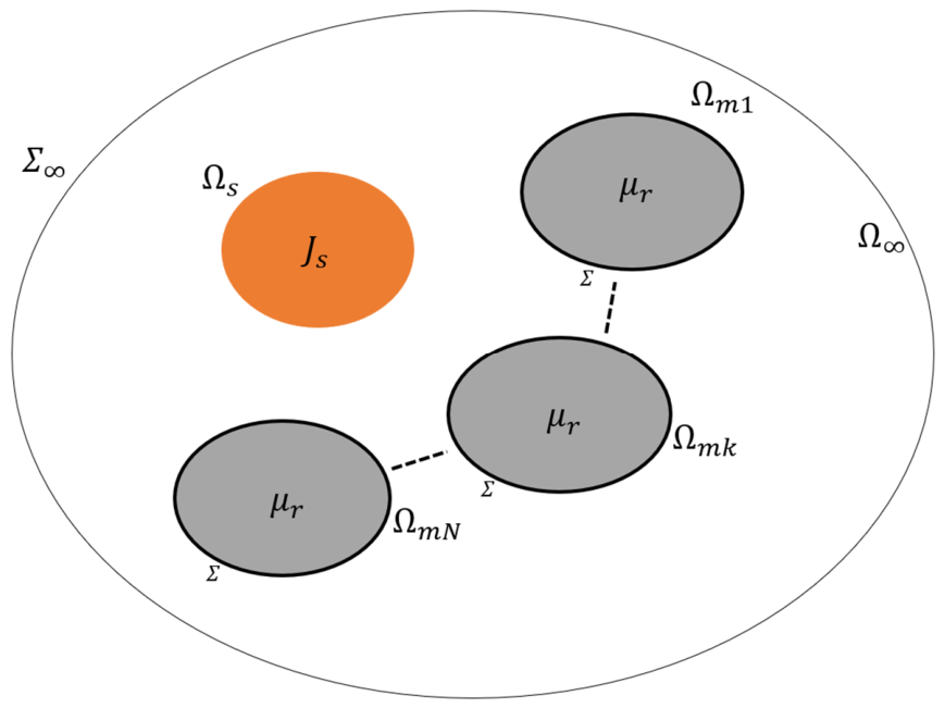
The reference problem is shown in Figure 1.
The reference formulation adopted to address the problem is the magnetostatic formulation of Maxwell’s equations:
× H = J s   i n   s 0   i n   s , · B = 0   everywhere
where Js is the current density, assigned in the region Ωs (the region occupied by the conductors), and H and B are, respectively, the magnetic field and the flux magnetic density. The computational domain is denoted by , whereas the regions m = k = 1 N m k are those occupied by the magnetic materials. Such materials are described by the generic constitutive equation:
B   =   μ 0   ( H   +   M ) ,
where μ0 = 4π·10−7 H/m is the magnetic permeability in the vacuum, and M is the magnetization. In the general case, M nonlinearly depends on the magnetic field H, and in the case of a linear material, it is
M =   ( μ r 1 ) H ,
where μ r is the relative magnetic permeability.
The continuity conditions on any surface Σ of discontinuity (on which it is assumed that there is no density of superficial current) impose that
H × n ^     c o n t i n u o u s   o n   Σ B · n ^     c o n t i n u o u s   o n   Σ .
Finally, the Σ standard Sommerfeld condition to infinity is assumed.
Considering a nonlinear constitutive relationship between M and H (hence, between B and H), the solution of the boundary value problem (1)–(4) usually requires a numerical solver that can be computationally demanding when associated with real-world structures. Indeed, the complex geometry of tokamak components requires fine spatial discretization in order to accurately capture the field gradients. Consequently, a careful geometrical simplification study is necessary to identify which features of the analyzed objects can be simplified and how to do so. This process aims at achieving a balance between constructing a mesh that includes all the relevant elements for an accurate field estimation and maintaining a number of elements low enough to avoid prohibitive computational costs.
This stage typically requires advanced expertise in both electromagnetic modeling and numerical discretization techniques. Moreover, the combination of high-resolution meshes and repeated nonlinear iterations leads to very demanding computational requirements. As a result, full numerical solutions are often impractical during the preliminary design phase, thereby motivating the development of the rapid estimation technique proposed in this work, which can be effectively applied even by engineers without specialized expertise in electromagnetic numerical modeling.
The state of the art of this approach is closely tied to the resolution capabilities of the finite element (FE) methods employed by the two software tools under consideration: ANSYS Maxwell and CARIDDI. While both tools utilize finite element methods (FEMs) for numerical analysis, they are founded on fundamentally different mathematical formulations. Specifically, ANSYS Maxwell is based on a differential formulation, whereas CARIDDI adopts an integral formulation. In this context, ANSYS Maxwell employs sparse matrices that are specifically tailored to reduce computational costs, with the number of elements also depending on the discretization of the air region. In contrast, CARIDDI uses dense matrices with a computational complexity of O(n2), while the overall problem solution scales as O(n3), making it considerably more demanding. However, unlike ANSYS Maxwell, the number of unknowns in CARIDDI is determined by the discretization of the magnetic materials and the sources; with this integral approach, the air region does not need to be discretized. However, these differences in formulation and discretization also affect how electromagnetic forces and torques are computed, since the accuracy of the field and current distributions determines the precision of the resulting load evaluations.
In particular, based on these formulations, force evaluation on the analyzed objects is carried out using the virtual work principle (used by ANSYS Maxwell) and Kelvin’s formulation (used by the CARIDDI code).
After the static problem is solved, the computation of the loads from the principle of virtual work is obtained by expressing the forces Fbody as follows:
F body = d W ( s , i ) ds i = const ,
where W is the magnetic co-energy of the system, i is the current, and s is the displacement.
Instead, when using Kelvin’s method, the forces are expressed by the following integral:
F k = V Mk M · μ 0 H extk   dV ,
where Hext,k represents the magnetic field generated by all external sources (such as the main coils and the other surrounding ferromagnetic components), explicitly excluding the self-field generated by the magnetization of the k-th volume VM,k itself. This exclusion is physically justified by the rigid body assumption: while the self-field does induce internal electromagnetic forces that tend to deform the material, these internal stresses inherently cancel out over the entire volume. Consequently, a rigid body cannot exert a net global force or torque on itself, meaning that only the interaction with the external field Hext,k contributes to the net magnetostatic loads transmitted to the mechanical supports.
The two force formulations present conceptual and numerical differences. The virtual work principle relies on the total magnetic co-energy of the system, offering a global and energetically consistent estimation of the mechanical loads. This makes it particularly robust in complex configurations, especially where the magnetic field exhibits strong spatial variations or localized nonlinearities.
Meanwhile, Kelvin’s method evaluates the force through a local interaction between the magnetization and the gradient of the external magnetic field. While more intuitive and straightforward in its physical interpretation, this formulation is sensitive to the accuracy of the field gradient estimation, which, in turn, depends heavily on the mesh quality and the regularity of the magnetic field.
From a modeling perspective, an important distinction between the two computational frameworks lies in the treatment of sources and domain discretization. When using an integral formulation (like in the Cariddi code), it is possible to efficiently handle both analytical and non-analytical excitations, such as an infinitely long wire. Instead, a differential formulation (like in ANSYS Maxwell) faces significant limitations in similar cases. In addition, integral methods require discretization only of the region containing the unknown source, implicitly satisfying boundary conditions and enabling independent refinement of different regions. They usually involve fewer unknowns but lead to full matrices, as their assembly relies on complex (often singular) integrals. Differential methods, in contrast, discretize the entire domain with a unified mesh, producing sparse local systems but requiring explicit boundary conditions and higher computational costs whenever the mesh is modified.
For fusion devices, integral formulations are especially advantageous: the large vacuum-to-specimen ratio significantly reduces the number of unknowns, and distant external sources (e.g., plasma modeled as a current-carrying wire) can be incorporated directly through their field contributions, without extending discretization to the whole domain.
The purpose of this work is to reduce the computational time required for magnetization evaluation, which is fundamental for force estimation. This is effectively achieved through an integral formulation that
(i)
Restricts discretization to the source region.
(ii)
Exploits the assumption that magnetization within this region is approximately uniform. Such efficiency is difficult to obtain with a differential approach, which requires computations across the entire (often very large) domain and cannot benefit from the uniform magnetization assumption, since the unknown is typically a potential.
While this approach is inherently less detailed than fully numerical methods, its strength lies in its ability to provide reliable order-of-magnitude estimates of the magnetostatic forces acting on the components under study, with a markedly lower computational cost. This enables even non-expert users to perform rapid evaluations—typically within a few minutes—to determine whether the forces involved are significant enough to justify further investigation, such as a detailed structural analysis.

2.2. Estimation of Ferromagnetic Forces via a Semi-Analytical Method

This section presents the core of the proposed approach: a semi-analytical method (hereafter, SA Method) for estimating magnetostatic forces acting on ferromagnetic components subjected to external magnetic fields. As already pointed out, the method is designed to offer a computationally efficient alternative to full nonlinear solvers, enabling rapid and reliable evaluations even for users with limited experience in advanced numerical modeling.
The method starts with a preliminary phase of geometry simplification. The components with magnetic properties are geometrically simplified in terms of uniformly magnetized hexahedrons. Each hexahedron is modeled with six faces, defined by their vertex coordinates and oriented counterclockwise, and is associated with its centroid position Pi = (xi, yi, zi) and dimensions dLi = (Lx, Ly, Lz).
The second phase is the evaluation of the magnetic field and vector potential generated by each hexahedron. This is based on the closed-form analytical expressions developed in [24], which describe the magnetostatic field of a uniform polyhedral source. These expressions have been implemented in a custom routine capable of computing the contributions of both uniform current density and uniform magnetization M within an arbitrary hexahedral volume. Specifically, for each face f of the hexahedron, the method computes the function ∇Wf as in [24]:
W f   r = e d g e f n ^ f   ×   t ^ e w e r n ^ f Ω f r
where t ^ e is the unit vector tangent to edge with endpoints r 1 and r 2 , and n ^ f is the unit vector normal to face, oriented according to the right-hand rule, with
w e r = ln r 2 r + r 1 r + r 2 r 1 r 2 r + r 1 r r 2 r 1
and Ω f r is the solid angle subtended to face f as seen from the point r . An analytical formula for Ω f r is reported in [24].
Having calculated (7), the magnetic flux density can be expressed as
B M = μ 0 4 π faces [ ( M × n ^ f ) × W f ] .
This formulation enables a precise and fully vector evaluation of magnetic interactions between hexahedrons.
It is important to highlight that the magnetic field is evaluated at the centroid of each hexahedral element. The total field is computed as the superposition of three components: the externally applied magnetic field, the self-induced field generated by the element’s own magnetization, and the contributions from the magnetization of neighboring hexahedrons. Moreover, the adopted formulation avoids singularities within the element itself, thereby enabling the direct and consistent evaluation of the self-field contribution.
The above-mentioned custom routine along with the auxiliary functions required for evaluating geometric integrals are available at the link provided in the final section, “Data Availability”.
In order to take into account a nonlinear magnetization law, it is useful to note that based on Equations (2) and (3), the magnetization M can be related to the local magnetic field B through the nonlinear constitutive relation:
M   =   ( 1 / μ 0 )   ( 1 1 / μ r ( B ) )   B .
The relative permeability μr(B) can be calculated from the material characterization, i.e., from the experimental B-H curve, by using the following expression:
μ r   =   | B | / ( μ 0 | H | ) .
Based on the above considerations, the distribution of the magnetization M is a solution of a nonlinear problem, that is, by means of a self-consistent iterative procedure, implementing the following steps:
  • Initialize the magnetization Mi for each hexahedron to an initial guess (e.g., zero values).
  • Compute the total magnetic field Btot(PiB) at the baricenter PiB of each hexahedron, defined as
    B tot ( P ) = B M ( P ) + B ext ( P ) ,
    where BM is given by (8), and Bext is the known external field.
  • Update the magnetization of each hexahedron using the nonlinear constitutive relation (10).
  • Check for convergence by comparing the norm of the iterative increment between Mi values at the steps n and n − 1:
    Δ M n = i | M i n M i n 1 | / | M i n | .
  • Repeat steps 2–4 until convergence is reached.
Note that the procedure converges in the case of monotonic and Lipschitz continuous B-H curves, as it happens in the cases of interest for our analysis [25,26].
Once the magnetization distribution is evaluated, the force is computed according to Kelvin’s method, as defined by Equation (6).

3. Case Study: Analysis and Discussion

This section presents a representative application case in the field of nuclear fusion, focusing on the ITER tokamak. The scenario involves strong magnetic fields interacting with ferromagnetic components, generating significant magnetostatic forces that can affect the structural integrity of the system.

3.1. Problem Description

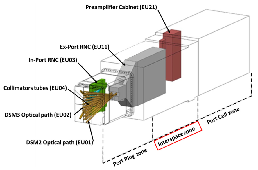
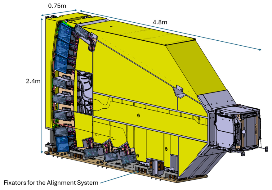
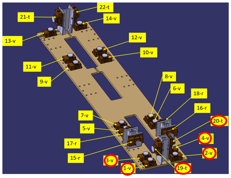
Within the ITER system, the Radial Neutron Camera (RNC) is a diagnostic designed to provide a time-resolved measurement of neutron and alpha source profile and the neutron power density [27]. It is composed of two fan-shaped collimating structures: the In-Port RNC, located inside the port plug of the ITER Equatorial Port #1 (EP01), and the Ex-Port RNC, located in the interspace zone of EP01 (see Figure 2) [28]. The Ex-Port RNC (identified as EU11) is a massive diagnostic subsystem (Figure 3) installed on the interspace supporting structure and is secured to the ground using a set of 22 mechanical supports known as fixators, positioned beneath the EU11 base plate (Figure 3 and Figure 4).
These components are critical in ensuring the mechanical alignment between the diagnostic subsystems. During the operation, the fixators must withstand the dead weight of the EU11 structure (17 t), the seismic loads and the influence of static magnetic fields generated during reactor operation. Thus, their main function is to anchor the EU11 to the ground, maintaining precise positioning throughout the device operational lifecycle.
In the following, the estimation of the ferromagnetic forces is carried out on a subset of six fixators corresponding to the positions closest to the plasma-facing side of the device (see Figure 4). For this reason, the selected supports are expected to experience the highest magnetic field gradients, and thus, the resulting forces provide a worst-case estimation of the loads acting on any of the fixators. Additional details on these supports are given in Appendix A.
The selected fixators are among the most critical components for analyzing ferromagnetic interactions due to their close proximity to the plasma and their expected exposure to the highest magnetic field intensities. Their geometric and mass properties (see Appendix A) serve as input parameters for subsequent numerical simulations aimed at estimating the magnetic forces acting on them.
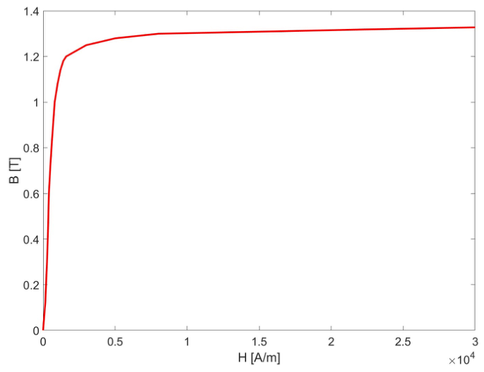
The fixators are made of a ferromagnetic gray cast iron, whose magnetic properties are described by the B–H curve in Figure 5, whose values at specific points of the curve are tabulated in Table 1.
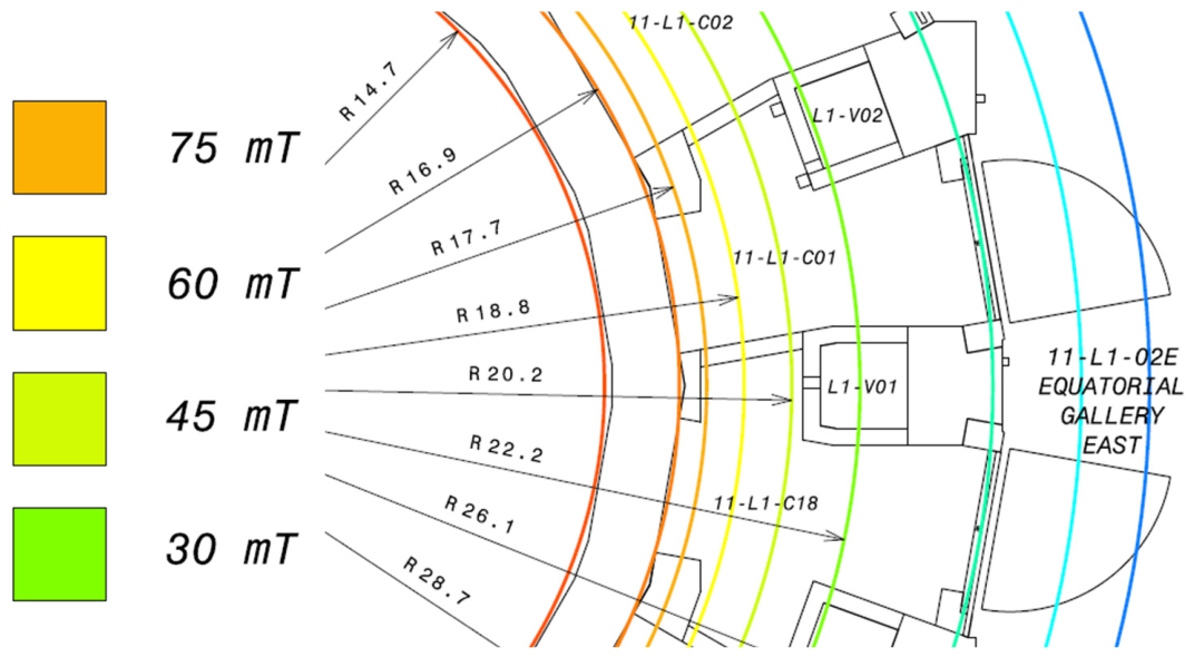
In order to determine the static magnetic field to be considered as the external excitation in this analysis, it is useful to refer to the map of the radial gradient of the B field reported in Figure 6, referring to the equilibrium 17 MA plasma scenario in ITER, in the global reference system.

3.2. Model Implementation

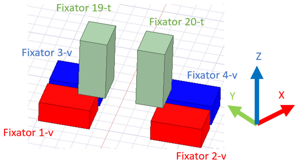
As pointed out in Section 2, the proposed model relies on a simplified representation of the fixators (see Figure 4), which are modeled as parallelepipeds (see Figure 7), preserving the same dimensions of the original supports (see Appendix A, Table A1).
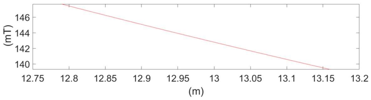
The external field to be imposed in the adopted model is derived by interpolating the values given in this map, considering the actual positions of the fixators in the global reference system. Specifically, since the selected fixators lie within a radial range from 12.75 m to 13.16 m in the global reference system, and the map in Figure 6 provides data only from a radial coordinate of 14.7 m onwards, a backward linear interpolation was applied to estimate the field in the region of interest. To this end, the slope of the field between two iso-field lines was first calculated and then used to reconstruct the spatial distribution of B in the target region, with the result given in Figure 8.
To summarize, the elements (fixators) to be considered in this analysis (Figure 4) are supports of a massive diagnostic module of the ITER reactor (EU11 in Figure 2), located outside the vessel at a distance of at least 12.75 m from the tokamak center. In this region, the field spatial distribution corresponding to the plasma equilibrium condition is given in Figure 5.

3.3. Results: Validation and Discussion

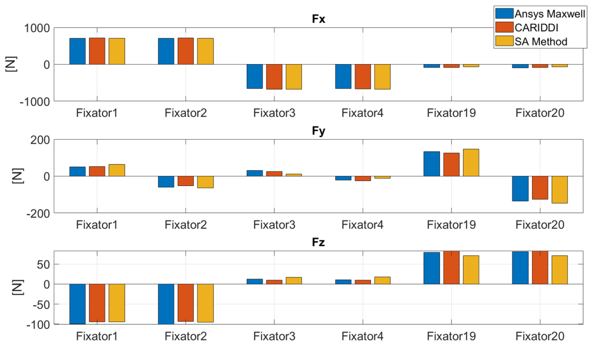
The results obtained by using the proposed semi-analytical method have been validated by comparing them with those provided by the cited Cariddi and Ansys-Maxwell tools. The computed values are compared in Table 2, referring to the three force components: Fx (radial), Fy (toroidal), and Fz (vertical). A visual representation of such results is also provided in the bar charts reported in Figure 9, organized by force components.
The comparative analysis highlights a very good qualitative agreement among the results obtained by the three approaches. In particular, for all the fixators and for all the force components, there is a perfect agreement in terms of force direction.
In terms of magnitude, note that for fixators 1 to 4, the radial component of the force, Fx, is the dominant contribution, being almost one order of magnitude larger than the other components. This component is estimated by the SA method with very high accuracy, with the difference from Maxwell and Cariddi results always being below 2%. In the case of fixators 19 and 20, the semi-analytical model shows more noticeable deviations, since the difference is now of the order of 19–25%. However, in this case, the Fx component is almost one order of magnitude lower compared with fixators 1–4; therefore, this higher error refers to smaller values. The Fz components are also well captured, while the Fy values of the fixators 1-v 2-v 19-t e 20-t tend to be slightly overestimated by the SA method compared with the numerical solvers. This confirms a good reliability of the semi-analytical method.
Overall, the SA method proves to be an extremely valuable tool for preliminary analysis, especially thanks to its very low computational cost; it requires only a few minutes to provide reasonably accurate force estimation. However, most important is the ease of use, since this estimation is carried out by running the routines provided in this paper (see final section, “Data Availability”), without the need for the expertise required to run simulation tools like those used here (Ansys or Cariddi).
The accuracy of the semi-analytical approach proposed here is fundamentally governed by the error introduced by assuming a uniform magnetization within each individual hexahedral block, rather than accounting for the actual spatial distribution of magnetization. In the case considered here, this error is approximately 5%, which is consistent with the field gradient in the region of interest. Indeed, the imposed external field exhibits a spatial variation of about 5% within this region (see Figure 5 and Figure 8).
It can be noted that the computed EM loads are the equivalent of 200–300 kg acting on a structure which weighs 16–17 tons, corresponding to a small fraction of the foreseen preloads of the bolts attaching the fixators to the baseplate (see Appendix B). For the sake of completeness, Table 3 reports the maximum load on each analyzed fixator resulting from the structural analyses performed on the Ex-Port RNC under the dimensioning load combination, which considers the occurrence of the seismic level 2 event during normal operating state conditions, with a fire event as a concatenated event (see Appendix B). The EM loads are again negligible, being two orders of magnitude less than the loads resulting from the structural analysis, and three orders less than the maximum admissible loads.

4. Conclusions and Future Works

This work presented and validated a semi-analytical method for a quick estimation of the ferromagnetic forces acting on magnetic objects under the effect of a known spatial gradient of the magnetic field. The proposed method is not meant to replace the accurate full numerical simulations carried out by using, for instance, FEM simulators, but rather, to serve as a practical tool in scenarios where an order-of-magnitude estimation of electromagnetic forces is sufficient. This may happen in cases where the electromagnetic effects are negligible compared with other possible sources of loads. However, the approach is valuable even in case the loads are comparable, since it provides a first and quick estimation of their magnitude.
The case study analyzed here was an example of conditions where the electromagnetic forces are negligible in the context of broader structural analyses that account for phenomena like seismic events. Specifically, the proposed method has been applied to estimate the forces acting on the supports of a component of a neutron diagnostic device to be used in the ITER tokamak. These forces arise from the interaction of the magnetic field generated in the tokamak and the magnetization of these supports, made of ferromagnetic material. The comparison between the results provided by the proposed method and those obtained by using two different full numerical tools satisfactorily validated the method.
While the accuracy of the proposed model is, in the general case, lower than that of full numerical solvers, it provides reliable estimates of the orders of magnitude with an approach that combines low computational costs and ease of use. Indeed, the proposed approach is implemented as routines provided in this paper, allowing users without specialized expertise in commercial simulation tools to estimate these forces effectively.
Future developments will focus on extending the model to account for material and geometric heterogeneities, while keeping computational costs manageable. This requires removing the current assumption of a uniform magnetization within the single block used in the model. In addition, a rapid estimation of the approximation error will be introduced, providing users with a quantitative measure of accuracy alongside the order-of-magnitude estimates, and thus offering a clearer indication of the reliability of the results.
Furthermore, future work will explore and validate the application of this rapid semi-analytical approach to magnetic problems in other industrially relevant sectors, such as industrial automation and the automotive industry, where fast and accessible preliminary evaluations are highly desirable.

Author Contributions

Conceptualization, A.M., A.G.C. and S.V.; methodology, G.D.M., A.G.C., S.V., E.O. and D.M. (Domenico Marzullo); formal analysis, A.M., S.V., D.M. (Domenico Marzullo) and B.E.; investigation, G.D.M., A.G.C., S.V. and E.O.; data curation, G.D.M., A.G.C., S.V., E.O. and D.M. (Domenico Marzullo), writing—original draft preparation, G.D.M. and A.G.C.; writing—review and editing, A.M., S.V., E.O., D.M. (Domenico Marzullo) and B.E.; supervision, A.M. and D.M. (Domenico Marzullo); project administration, D.M. (Daniele Marocco); funding acquisition, B.E. and D.M. (Daniele Marocco). All authors have read and agreed to the published version of the manuscript.

Funding

The work leading to this publication was funded partially by Fusion for Energy under the Specific Grant Agreement F4E-FPA-327 SG07. This publication reflects the views only of the author, and Fusion for Energy or ITER Organization cannot be held responsible for any use which may be made of the information contained therein.

Institutional Review Board Statement

Not applicable.

Informed Consent Statement

Not applicable.

Data Availability Statement

The routines developed for implementing the proposed method are freely available at the GitHub repository at the link: https://github.com/achiariello/fastforce (accessed on 8 June 2026). The simulation data are available upon request to the corresponding author.

Acknowledgments

During the preparation of this manuscript, the authors used ANSYS Maxwell, R24.1 and the proprietary code CARIDDI for the purpose of performing electromagnetic analyses used to validate the proposed method. Additionally, the authors used the AI tool ChatGPT (OpenAI, GPT-4o) to assist in checking and rephrasing the English language in some parts of the written text.

Conflicts of Interest

The authors declare no conflicts of interest.

Abbreviations

The following abbreviations are used in this manuscript:
ITERInternational Thermonuclear Experimental Reactor
DEMODEMOnstration Power Plant
FEMFinite Element Method
SA MethodSemi-Analytical Method
EMElectromagnetic
RNCRadial Neutron Camera
EU11Embarked Units 11
FLCSFixator Local Coordinate System

Appendix A. Details on the Fixators

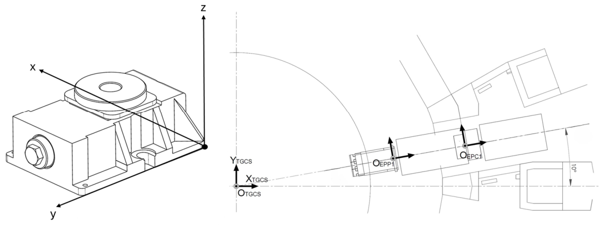
The fixators selected for the analysis carried out in this work are highlighted in red in Figure 4, along with the identification label. Their spatial configuration is defined with respect to a Fixator Local Coordinate System (FLCS). The origin of each FLCS is centered on the point shown in Figure A1, whose coordinates (x, y, z) are reported in Table A1 and refer to the ITER Equatorial Port #1 Coordinate System. This system is located at the origin of the Tokamak Global Coordinate System but rotated 10° counter-clockwise around the z-axis to match the EP01 toroidal orientation, as shown in Figure A1 (left).
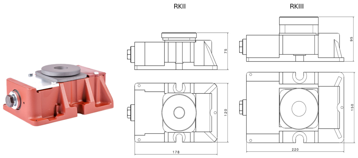
Table A1 also provides the mass and dimensions (Lx, Ly and Lz) of each side of the considered fixator, as also shown in Figure A2. It can be noted that the fixators are grouped by dimension into two different types, RKII and RKIII.
Figure A1. Details of the fixator showing the considered Fixator Local Coordinate System (FLCS) (left) and the Equatorial Port #1 Coordinate System (right).
Applsci 16 06099 g0a1
Table A1. Coordinates and dimensions of the selected fixators (in the FLCS).
Objectx [mm]y [mm]z [mm]Lx, Ly, Lz [mm]Fixator SizeMass [kg]
Fixator 1-v12,756196−392(120, 178, 75)RKII5.5
Fixator 2-v12,756−196−392(120, 178, 75)RKII5.5
Fixator 3-v12,900196−392(120, 178, 75)RKII5.5
Fixator 4-v12,900−196−392(120, 178, 75)RKII5.5
Fixator 19-t12,748142−250(150, 95, 220)RKIII11.5
Fixator 20-t12,748−60−250(150, 95, 220)RKIII11.5
Figure A2. Example of a fixator (left) and main dimensions of the RKII and RKIII fixators (right).
Applsci 16 06099 g0a2

Appendix B. Loads Associated with the ITER RNC

The main loads that are identified for the study of the ITER RNC components are summarized in Table A2.
Table A2. Summary of the main loads acting on the ITER-RNC components.
Load CaseLoads
Dead weightGravity (9.81 m/s2) acceleration acting on components masses (DW). RNC total mass: 17,000 Kg
Assembly or installation loadsBolts preload (75% yield of bolts material as first guess) −59 kN
DW acting on eyebolt during installation.
Seismic eventsFloor response spectra (FRS) for seismic level SL-2
Zero-period acceleration: ax = 7.3 m/s2, ay = 8.7 m/s2, and az = 13.3 m/s2
Operational loadsCoolant pressure: 1 MPa
Environmental pressure: atmospheric pressure (1 × 10⁵ Pa)
He4 detector pressure: 10 MPa
Environmental EM loadAs calculated in this paper
Thermal and nuclear loadsInterspace environment: T(Min/Max) = 5/35 °C; HTC = 5 W/m2K
Coolant: Tinlet = 34 °C; MFR = 1.15 Kg/s
Volumetric nuclear heating
Dose on detectors, sensors and electrical components
Accident and incident loadsEx-vessel loss-of-cooling accident (LOCA).
Max. environment T = 145 °C; HTC = 5 W/m2K
Max. P = 160 kPa.
Internal fire: survive at 300 °C for two hours

References

  1. Wesson, J.; Campbell, D.J. Tokamaks; Oxford University Press: Oxford, UK, 2011. [Google Scholar]
  2. Lawson, J.D. Some criteria for a power producing thermonuclear reactor. Proc. Phys. Soc. Sect. B 1957, 70, 6–10. [Google Scholar] [CrossRef] [Scilit]
  3. EAST (HT-7U), in Hefei, China. Available online: http://english.hf.cas.cn/ic/ip/east/ (accessed on 9 February 2026).
  4. Ko, W.-H.; Yoon, S.; Kim, W.; Kwak, J.; Park, K.; Nam, Y.; Wang, S.; Chung, J.; Park, B.; Park, G.; et al. Overview of the KSTAR experiments toward fusion reactor. Nucl. Fusion 2024, 64, 112010. [Google Scholar] [CrossRef] [Scilit]
  5. Ishida, S.; Barabaschi, P.; Kamada, Y. Overview of the JT-60SA project. Nucl. Fusion 2021, 51, 094018. [Google Scholar] [CrossRef] [Scilit]
  6. Shimomura, Y.; Aymar, R.; Chuyanov, V.; Huguet, M.; Parker, R.; ITER Joint Central Team. TER overview. Nucl. Fusion 1999, 39, 1295. [Google Scholar] [CrossRef] [Scilit]
  7. Federici, G.; Kemp, R.; Ward, D.; Bachmann, C.; Franke, T.; Gonzalez, S.; Lowry, C.; Gadomska, M.; Harman, J.; Meszaros, B.; et al. Overview of EU DEMO design and R&D activities. Fusion Eng. Des. 2014, 89, 882–889. [Google Scholar] [CrossRef] [Scilit]
  8. Freidberg, J.P. Ideal Magnetohydrodynamics; Plenum: New York, NY, USA, 1987. [Google Scholar]
  9. Noce, S.; Dose, G.; Flammini, D.; Imbriani, V.; Mazzone, G.; Moro, F.; Roccella, S.; Romanelli, F.; Villari, R.; Visca, E.; et al. Nuclear analyses for the design of the ITER-like plasma facing components vertical targets of the DEMO divertor. Fusion Eng. Des. 2020, 155, 111730. [Google Scholar] [CrossRef] [Scilit]
  10. Di Maio, P.A.; Mazzone, G.; Quartararo, A.; Vallone, E.; You, J. On the thermal-hydraulic performances of the DEMO divertor cassette body cooling circuit equipped with a liner. Fusion Eng. Des. 2020, 156, 111613. [Google Scholar] [CrossRef] [Scilit]
  11. Mazzone, G.; You, J.-H.; Cerri, V.; Coccorese, D.; Garitta, S.; Di Gironimo, G.; Marzullo, D.; Di Maio, P.; Vallone, E.; Tincani, A.; et al. Structural verification and manufacturing procedures of the cooling system for DEMO divertor target (OVT). Fusion Eng. Des. 2019, 146, 1610–1614. [Google Scholar] [CrossRef] [Scilit]
  12. Mazzone, G.; You, J.-H.; Bachmann, C.; Bonavolontà, U.; Cerri, V.; Coccorese, D.; Dongiovanni, D.; Flammini, D.; Frosi, P.; Forest, L.; et al. Eurofusion-DEMO-cassette design and integration. Fusion Eng. Des. 2020, 157, 111656. [Google Scholar] [CrossRef] [Scilit]
  13. Mazzone, G.; Sannazzaro, G.; Schioler, T.; Sorin, V. Seismic design of the ITER main Tokamak components. Fusion Eng. Des. 2011, 86, 1984–1988. [Google Scholar] [CrossRef] [Scilit]
  14. Boozer, A.H. Theory of tokamak disruptions. Phys. Plasmas 2012, 1, 058101. [Google Scholar] [CrossRef] [Scilit]
  15. Di Mambro, G.; Maffucci, A.; Mazzone, G.; Ventre, S.; Villone, F.; You, J. Mechanical impact of electromagnetic transients on the European DEMO divertor. Part 1: Vertical displacement event. Fusion Eng. Des. 2022, 175, 112999. [Google Scholar] [CrossRef] [Scilit]
  16. You, J.; Mazzone, G.; Visca, E.; Greuner, H.; Fursdon, M.; Addab, Y.; Bachmann, C.; Barrett, T.; Bonavolontà, U.; Böswirth, B.; et al. Divertor of the European DEMO: Engineering and technologies for power exhaust. Fusion Eng. Des. 2022, 175, 113010. [Google Scholar] [CrossRef] [Scilit]
  17. Laghi, D.; Fabbri, M.; Cubi, A.; Pampin, R.; Pedroche, G.; Alguacil, J.; Garcia, J.; Catalan, J.; Portone, A. Comprehensive assessment of nuclear heating in ITER superconducting magnets using a full-tokamak 360° model. Fusion Eng. Des. 2025, 213, 114879. [Google Scholar] [CrossRef] [Scilit]
  18. Di Mambro, G.; Maffucci, A.; Mazzone, G.; Rubinacci, G.; Ventre, S.; Villone, F.; You, J. Ferromagnetic forces acting on the EU-DEMO divertor. Fusion Eng. Des. 2023, 190, 113522. [Google Scholar] [CrossRef] [Scilit]
  19. Albanese, R.; Calvano, F.; Mut, G.D.; Ferraioli, F.; Formisano, A.; Marignetti, F.; Martone, R.; Romano, A.; Rubinacci, G.; Tamburrino, A.; et al. Coupled Three Dimensional Numerical Calculation of Forces and Stresses on the End Windings of Large Turbo Generators via Integral Formulation. IEEE Trans. Magn. 2012, 48, 875–878. [Google Scholar] [CrossRef]
  20. Lee, S.-H.; Park, I.-H.; Lee, K.-S. Comparison of mechanical deformations due to different force distributions of two equivalent magnetization models. IEEE Trans. Magn. 2000, 36, 1368–1372. [Google Scholar] [CrossRef] [Scilit]
  21. Available online: www.ansys.com (accessed on 8 June 2026).
  22. Albanese, R.; Rubinacci, G. An integral formulation for. 3-D eddy current computation using edge elements. IEE Proc. A 1988, 135, 457–462. [Google Scholar] [CrossRef] [Scilit]
  23. Sannazzaro, G.; Bachmann, C.; Campbell, D.J.; Chiocchio, S.; Girard, J.; Gribov, Y.; Reyes, S.; Sugihara, M.; Tada, E.; Taylor, N. Structural load specification for ITER tokamak components. In Proceedings of the 2009 23rd IEEE/NPSS Symposium on Fusion Engineering, San Diego, CA, USA, 1–5 June 2009; pp. 1–4. [Google Scholar] [CrossRef] [Scilit]
  24. Fabbri, M. Magnetic Flux Density and Vector Potential of Uniform Polyhedral Sources. IEEE Trans. Magn. 2008, 44, 32–36. [Google Scholar] [CrossRef] [Scilit]
  25. Hantila, F.I.; Preda, G.; Vasiliu, M. Polarization method for static fields. IEEE Trans. Magn. 2000, 36, 672–675. [Google Scholar] [CrossRef] [Scilit]
  26. Albanese, R.; Rubinacci, G. Finite Element Methods for the Solution of 3D Eddy Current Problems. Adv. Imaging Electron Phys. 1997, 102, 1–86. [Google Scholar] [CrossRef] [Scilit]
  27. Esposito, B.; Marocco, D.; Gandolfo, G.; Belli, F.; Bertalot, L.; Blocki, J.; Bocian, D.; Brolatti, G.; Cecconello, M.; Centioli, C.; et al. Progress of design and development for the ITER radial neutron camera. J. Fusion Energy 2022, 41, 22. [Google Scholar] [CrossRef] [Scilit]
  28. Marzullo, D.; Occhiuto, E.; Brolatti, G.; Falco, D.; Laghi, D.; Marocco, D.; Esposito, B. Mechanical design of ITER radial neutron camera Ex-Port system. Fusion Eng. Des. 2024, 203, 114477. [Google Scholar] [CrossRef] [Scilit]
Figure 1. Reference geometry of magneto-static problem.
Applsci 16 06099 g001
Figure 2. Overall view of the ITER RNC diagnostic, with the EU11 location (interspace zone) highlighted in red [27].
Applsci 16 06099 g002
Figure 3. Details of the EU11 subsystem with a view of the base plate including the fixators.
Applsci 16 06099 g003
Figure 4. Yellow arrows indicate the location of the 22 fixators; those analyzed in the present work are highlighted in red.
Applsci 16 06099 g004
Figure 5. The nonlinear magnetization B–H curve of the considered ferromagnetic cast iron.
Applsci 16 06099 g005
Figure 6. Radial gradient of the B field for the 17 MA plasma scenario in ITER.
Applsci 16 06099 g006
Figure 7. Simplified fixator geometry adopted for the proposed method.
Applsci 16 06099 g007
Figure 8. Backward linear interpolation of the radial magnetic field in the region where the analyzed fixators lie.
Applsci 16 06099 g008
Figure 9. Bar charts comparing the results of the three approaches for each force component.
Applsci 16 06099 g009
Table 1. Some specific values of the B–H curve in Figure 5.
H [A/m]B [T]
00
2700.3
4000.6
8001.0
16001.2
80001.3
16,0001.3101
30,0001.3276
Table 2. Ferromagnetic forces acting on the selected fixators computed from the proposed method (SA method) and compared with those provided by the Ansys Maxwell and Cariddi tools.
Ansys MaxwellCariddiSA Method
FixatorFx [N]Fy [N]Fz [N]Fx [N]Fy [N]Fz [N]Fx [N]Fy [N]Fz [N]
1-v70851−10071753−9470864−94
2-v705−59−101714−53−93707−64−95
3-v−6593012−6732610−67711.417
4-v−658−2211−670−2610−676−11.318
19-t−8613479−8712583−6914671
20-t−93−13581−87−12583−69−14671
Table 3. Electromagnetic loads (total values of the force) compared with the values coming from the structural analysis and the maximum admissible load.
EM (SA Method)Structural AnalysisMaximum Admissible
Fixator[kN][kN][kN]
1-v0.7270710
2-v0.7274.1710
3-v0.68202710
4-v0.68123710
19-t0.1871710
20-t0.1896710
Disclaimer/Publisher’s Note: The statements, opinions and data contained in all publications are solely those of the individual author(s) and contributor(s) and not of MDPI and/or the editor(s). MDPI and/or the editor(s) disclaim responsibility for any injury to people or property resulting from any ideas, methods, instructions or products referred to in the content.