Distributed Relaxation Spectrum Delay Differential Model for Viscoelastic Materials: Stability and Bifurcation Analysis

Abstract

In our research, we developed a Distributed Relaxation Spectrum Delay Differential Equation (DRSDDE) model to simulate viscoelastic responses exhibited by materials with multiple-scale relaxation mechanisms and finite delay times. Our model expanded upon traditional integer-order viscoelastic models to include a continuum relaxation process using a log-time-space Gaussian distribution representing a continuum of relaxation processes, including a direct representation of the effect of delayed feedback via an explicit time delay term. Consequently, the resultant model can be viewed as a generalized Maxwell-type formulation where the viscoelastic behavior exhibits distributed relaxation dynamics and has finite signal propagation characteristics. We then used experimental data obtained from three representative materials: PDMS Sylgard 184, bovine brain white matter, and polyurethane foam to calibrate the model. Calibration was achieved by estimating model parameters through the use of Gauss-Legendre quadrature combined with non-linear optimization of the relaxation spectrum. The results indicate that the coefficients of determination for each of the materials exceeded $R^2>0.83$. Therefore, the proposed DRSDDE model outperformed the classical Zener model when simulating materials that exhibit a wide relaxation spectrum. The parameter values estimated for each of the examined materials provided additional insight into their physical behaviors. Specifically, the characteristic relaxation times for the studied materials were determined based upon ${\tau }_c= {10}^{\mu }$ ranging from about 63 s to 158 s. These results illustrate different dominant relaxation regimes for the investigated materials. Additionally, both characteristic equations and frequency domain analyses were utilized to study the stability and bifurcation properties of the DRSDDE model. A significant finding resulted from identifying a delay-insensitive stability regime for materials with $\tilde{K}< 1$ (as illustrated by bovine brain white matter). For materials with $\tilde{K} > 1$, the analysis revealed Hopf bifurcation results illustrating critical delay thresholds and frequencies for the onset of oscillations. Further, it was established that all calibrated delay values were significantly less than these threshold values. This indicates that all identified models functioned well below the oscillation thresholds at realistic delay times. Ultimately, the proposed DRSDDE model represents a physically intuitive, robust, and flexible method for modeling complex viscoelastic systems. Future research will involve investigating temperature-dependent effects, nonlinear bifurcations, and experimental validations of predicted oscillatory dynamics.

1. Introduction and Literature Review

The mechanical characteristics of viscoelastic materials include memory (i.e., history) effects, hereditary damping, and multi-scale relaxation. This type of material is used throughout many engineering disciplines, e.g., polymers, biological tissue, asphalt concrete, and advanced composites. Traditional elastic/anelastic constitutive models are inadequate for capturing the long-term memory and multi-scale relaxation behaviors that occur in these types of materials. Mechanical analogue models of viscoelastic behavior have been historically described using the framework of classical elastic/anelastic theories. Specifically, William Thomson and Woldemar Voight were among the first to develop mechanical analogs of time-dependent material behavior consisting of a combination of elastic springs and viscous dashpots [1,2]. Clarence Zener’s Standard Linear Solid model was later developed to further improve upon these concepts with regard to describing both stress relaxation and creep properties of solids [3].

Although they were central to developing early viscoelastic theories, most classical models are limited by their assumption of a single characteristic relaxation time and do not well capture the multiscale nature of the relaxation phenomena that occur in many real materials. A number of comparative studies show that integer-order constitutive relations cannot accurately predict the power-law relaxation behaviors found in polymer systems as well as some composite materials [4]. Therefore, researchers have pursued other methods to model long memory effects.

Fractional calculus is an important and relatively recent development in mathematics used to model memory-dependent properties of materials. The first application of fractional calculus was made by Michele Caputo, who incorporated fractional derivatives into constitutive equations in order to account for dissipation characterized by nearly frequency-independent attenuation [5]. Later, through collaborations with Francesco Mainardi, it was shown that fractional operators naturally produce power-law decay (relaxation) and hereditary effects consistent with experimentally observed behavior in viscoelastic materials [6]. Fractional constitutive equations have also been effectively applied to the analysis of the transient response of structures containing viscoelastic damping by R. L. Bagley and P. J. Torvik [7].

Fractional differential equations and their applications to physical systems were further developed in the work of Igor Podlubny [8], on which subsequent investigations have been based that demonstrated that rheological models provide continuous interpolation between elastic and viscous responses, thus providing one unified description of creep, relaxation, and viscosity over multiple time scales. Fractional viscoelastic models have been utilized throughout solid mechanics [9] and materials science [10] to describe anomalous dissipative processes and complex relaxation behavior within viscoelastic media. A comprehensive mathematical treatment of wave propagation in hereditary media has been provided by Francesco Mainardi in his monograph on fractional viscoelasticity [11].

While fixed-order fractional derivatives are an improvement upon the classical models (e.g., Newtonian viscosity), several classes of materials will typically exhibit relaxation spectra that cannot be modeled well using a single value for the fractional order. One way to model the relaxation spectra exhibited by a material with multiple relaxations was through the use of “distributed relaxation spectrum” fractional models. Distributed relaxation spectrum fractional models treat the derivative order as a variable and integrate it over some distribution. The first theoretical study that used distributed relaxation spectrum fractional models to represent dissipative processes in both dielectric and diffusive systems was performed by Michele Caputo [12] when he introduced the concept of distributed relaxation spectrum differential equations. Studies by Chechkin et al. later showed that distributed relaxation spectrum fractional models provided a flexible means of modeling anomalous diffusion and multiscale relaxation phenomena [13]. Additionally, Atanacković et al. developed constitutive relations using distributed relaxation spectrum viscoelastic models. They demonstrated that Distributed relaxation spectrum fractional models could model a broader range of relaxation mechanisms than traditional fixed-order models [14]. Most recently, variable- and distributed relaxation spectrum fractional models have been applied to linear viscoelasticity to model materials with varying properties depending on either their memory characteristics over time or their deformation regime [15].

Time delays can occur in viscoelastic systems because of relaxation processes, delayed feedback loops, or slow signal propagation through heterogeneously structured materials. Delay-Differential Equations (DDEs) provide a mathematically rigorous approach to studying these types of systems. Jack K. Hale and Jean-Pierre Lunel’s work on Functional Differential Equations (FDEs) has provided numerous results regarding the existence, stability, and bifurcation of DDEs [16]. A further contribution was made by Thierry Erneux, who systematically studied how DDEs induce oscillatory behavior in nonlinear systems via Hopf Bifurcations [17].

In terms of Control Theory, many researchers (including Silviu-Iulian Niculescu) have investigated the effects of time delays upon system stability. He was able to demonstrate that time delays could cause an otherwise stable system to become unstable and create Oscillations [18]. Gu et al. also provided further analytical work based on Frequency-Domain and Lyapunov Methods to determine the stability of Delay Systems [19], and Michiels and Niculescu presented methods to use the Eigenvalues to assess the stability and stabilization of such delay systems [20]. Finally, researchers have published Surveys detailing Modern Developments in both the delay-dependent analysis of stability and the design of controls for dynamical systems containing delays [21].

Although there is an abundance of research related to fractional viscoelastics as well as time-delayed systems, very little has been done to develop or investigate models that include both distributed relaxation spectrum memory and explicit time delays. One area in particular where limited research exists is the study of stability and bifurcations due to the inclusion of delay terms in DRSDDEs describing viscoelastic behavior. This paper will address this shortcoming through the development of a distributed relaxation spectrum Delay Differential Equation (DRSDDE) model for viscoelastic materials and a comprehensive analysis of the DRSDDE’s stability and delay-induced bifurcation behavior.

The main results of this work can be stated as follows. First, we develop a distributed relaxation spectrum delay differential equation model for describing viscoelastic materials that exhibit multiscale relaxational processes. Second, the stability conditions are determined using characteristic-equation methods and frequency-domain analyses. Third, we describe and investigate how the delay-induced Hopf bifurcation depends on the distributed relaxation spectrum. Fourth, we present some simulation examples illustrating the dynamics of the proposed model and demonstrating its ability to generate an important variety of complex relaxational patterns in comparison to well-established viscoelastic models.

2. Mathematical Preliminaries

In this section, we briefly review several mathematical concepts required for the formulation and analysis of the proposed distributed relaxation spectrum delay differential equation model.

2.1. Classical Viscoelastic Models

The early theoretical foundations for viscoelastic theory are derived from both classical (elastic) and anelastic solid deformation theories. Models that were developed during this time period to establish the fundamental relationships or “constitutive equations” that describe the elastic behavior of materials and the presence of internal friction were referred to as Zener models. One of the most well-known and earliest examples of a viscoelastic model is the Kelvin-Voigt model, which consists of a spring and a dashpot in series. This is represented by the constitutive equation shown below:

$$\sigma \left(t\right)=E \epsilon \left(t\right)+\eta {\displaystyle \frac{d\epsilon \left(t\right)}{dt}}$$

(1)

where $\sigma \left(t\right)$ is stress, $\epsilon \left(t\right)$ is strain, $E$ is Young’s modulus, and $\eta$ is viscosity. While this model captures instantaneous elastic response and viscous damping, it cannot model stress relaxation, a fundamental characteristic of viscoelastic materials.

The Zener model (Standard Linear Solid), consisting of a spring in series with a spring-dashpot parallel combination, overcomes this limitation by

$$\sigma \left(t\right)+{\tau }_{\sigma }{\displaystyle \frac{d\sigma \left(t\right)}{dt}}=E_0\left[\epsilon \left(t\right)+{\tau }_{\epsilon }{\displaystyle \frac{d\epsilon \left(t\right)}{dt}}\right]$$

(2)

where ${\tau }_{\sigma }$ and ${\tau }_{\epsilon }$ are relaxation and retardation times and $E_0$ is the elastic modulus. This model exhibits exponential stress relaxation and creep recovery, making it more realistic for many materials. However, both models assume a single relaxation time and cannot capture the multi-scale relaxation phenomena observed in complex materials.

2.2. Fractional Viscoelastic Models

The fractional calculus framework has emerged as a powerful tool for addressing the limitations of classical models. Fractional derivatives naturally encode power-law relaxation and nonlocal temporal behavior. Among several definitions of fractional derivatives, the Caputo derivative is widely used in physical applications due to its compatibility with classical initial conditions. The Caputo fractional derivative of order $\alpha \in \left(0, 1\right)$ is defined as;

$${}_{ }{}^{C}D_t^{\alpha } f\left(t\right)={\displaystyle \frac{1}{\mathsf{\Gamma }(1-\alpha )}}{\int }_0^t{\displaystyle \frac{f^{\prime }\left(\tau \right)}{{\left(t-\tau \right)}^{\alpha }}}d\tau$$

(3)

which has the Laplace transform $L\left\{{}_{ }{}^{C}D_t^{\alpha } f\left(t\right)\right\}=s^{\alpha }F\left(s\right)-s^{\alpha -1}f\left(0\right)$, enabling frequency-domain analysis. $L\{·\}$ denotes the Laplace transform operator, $F\left(s\right)$ is the Laplace transform of $f\left(t\right),$ $\Gamma (·)$ denotes the Gamma function and $s$ is the complex Laplace variable.

Fractional viscoelastic models replace the integer-order derivatives in classical models with fractional operators. For example, the fractional Zener model is

$$\sigma \left(t\right)+{\tau }_{\sigma }{}_{ }{}^{C}D_t^{\alpha } \sigma \left(t\right)=E_0\left[\epsilon \left(t\right)+{\tau }_{\epsilon }{}_{ }{}^{C}D_t^{\alpha } \epsilon \left(t\right)\right]$$

(4)

Foundational studies established that fractional derivatives provide a continuous interpolation between pure elastic and pure viscous responses. Subsequent analysis demonstrated the effectiveness of fractional rheological models in describing fractional relaxation processes and anomalous dissipation in a wide class of viscoelastic materials. Fractional viscoelastic models have been successfully applied to polymers, biological tissues, and composite materials.

2.3. Distributed Relaxation Spectrum, Fractional Models

Distributed relaxation spectrum fractional formulations have been widely proposed to model materials exhibiting a spectrum of relaxation behaviors. A typical representation is given by

$${\displaystyle \underset{0}{\overset{1}{\int }}}\rho \left(\alpha \right) \left(\sigma \left(t\right)+{\tau }_{\sigma }{}_{ }{}^{C}D_t^{\alpha } \sigma \left(t\right)\right)d\alpha =E_0\left({\displaystyle \underset{0}{\overset{1}{\int }}}\rho \left(\alpha \right)\left(\epsilon \left(t\right)+{\tau }_{\epsilon }{}_{ }{}^{C}D_t^{\alpha } \epsilon \left(t\right)\right)d\alpha \right)$$

(5)

In this framework, the contribution of fractional derivatives of different orders is weighted by a non-negative distribution function $\rho \left(\alpha \right),$ for $\alpha \in \left(0, 1\right)$. The weight function is assumed to satisfy the normalization condition ${\displaystyle {\int }_0^1}\rho \left(\alpha \right)d\alpha =1,$ which ensures that the distributed relaxation spectrum operator represents a convex combination of fractional dynamics.

The distributed relaxation spectrum formulation enables the model to capture multi-scale relaxation behavior that a single fractional exponent cannot describe. This approach is particularly well-suited for complex viscoelastic materials characterized by heterogeneous microstructures or evolving relaxation spectra.

Typical choices for the weight function include a uniform distribution $\rho \left(\alpha \right)=1,$ for $\alpha \in \left(0, 1\right),$ which assigns equal importance to all fractional orders, Beta-type distribution

$$\rho \left(\alpha \right)={\displaystyle \frac{\mathsf{\Gamma }\left(p+q\right)}{\mathsf{\Gamma }\left(p\right)\mathsf{\Gamma }\left(q\right)}}{\alpha }^{p-1}{(1-\alpha )}^{q-1},$$

which allows preferential weighting of specific relaxation scales through the parameters $p,q>0$. As a limiting case, the Dirac delta distribution $\rho \left(\alpha \right)=\delta \left(\alpha -{\alpha }_0\right)$ reduces the distributed relaxation spectrum formulation to the classical single-order fractional model of order ${\alpha }_0\in \left(0, 1\right).$

For analytical clarity, the subsequent stability and bifurcation analysis is carried out for admissible weight functions $\rho \in L^1\left(0, 1\right),$ where $L^1\left(0, 1\right)$ denotes the space of absolutely integrable functions on (0, 1). This assumption ensures the well-definedness of the distributed relaxation spectrum operators and facilitates the application of characteristic equations and frequency-domain techniques.

However, despite their modeling flexibility, distributed relaxation spectrum fractional formulations introduce significant mathematical complexity and may not always provide clear physical interpretability in terms of classical viscoelastic mechanisms. In particular, the relationship between distributed fractional operators and standard relaxation spectra remains an active area of research.

For this reason, in the present work, we adopt an alternative formulation based on a continuous spectrum of classical relaxation modes, which allows a more direct physical interpretation and facilitates stability analysis.

2.4. Time Delay Effects in Viscoelastic Systems

The time delay $(\tau > 0)$ reflects the delayed responses associated with viscoelastic material properties. Time delays can be due to a variety of factors such as slow restructuring processes within the microscopic structure, long-distance intermolecular interactions, or internal feedback loops. It has been well established that time-delayed systems have a significant impact on system stability and potentially generate oscillations or bifurcations that would otherwise not exist.

Delay differential equations (DDEs) have been extensively studied in control theory and dynamical systems. A general linear delay differential equation with a single discrete delay can be written as

$$\dot{x}\left(t\right)=Ax\left(t\right)+Bx(t-\tau )$$

where $A$ and $B$ are constant coefficients and $x\left(t\right)$ is the state vector. The stability of DDE is determined by the characteristic equation $\det \left(\lambda I-A-B{e}^{-\lambda \tau }\right)=0.$ Here, $\lambda$ is the characteristic eigenvalue and $I$ denotes the identity matrix. As the delay $\tau$ increases, eigenvalues cross the imaginary axis, leading to bifurcations. Hopf Bifurcation occurs when a pair of complex conjugate eigenvalues cross the imaginary axis, producing periodic oscillations. Studies on time-delayed fractional order systems have shown that there are many different ways that delays can induce Hopf Bifurcations, switching in stability, and produce rich dynamic responses.

However, the amount of work done on distributed relaxation spectrum systems with delays has been very limited. In this paper, we consider a constant time delay, which represents the common type of response lag experienced by viscoelastic materials. We assume a constant time delay because it allows us to obtain an analytical solution for our model and retains all the important dynamic effects caused by the delayed material response.

3. Distributed Relaxation Spectrum Delay Differential Equation (DRSDDE) Model

We now introduce the proposed Distributed Relaxation Spectrum Delay Differential Equation (DRSDDE) constitutive model for viscoelastic materials. The model establishes a generalized stress–strain relationship that incorporates distributed relaxation spectrum relaxation mechanisms and explicit time-delay effects within a unified constitutive framework.

Note that, throughout the remainder of the paper, $\tau$ denotes a generic delay parameter appearing in the theoretical model. The symbol ${\tau }_d$ denotes the calibrated delay obtained from parameter identification, while ${\tau }_c={10}^{\mu }$ denotes the characteristic relaxation time associated with the center of the Gaussian relaxation spectrum. Critical Hopf delays are denoted by ${\tau }_c^{\left(n\right)}$.

3.1. Continuous Relaxation Spectrum Representation

We represent the stress as a superposition of relaxation modes parameterized by a continuous variable $\alpha \in (0, 1)$ to accurately capture the multi-scale nature of viscoelastic relaxation. Each mode corresponds to a Maxwell-type element with its own relaxation rate. The total stress is defined as

$$\sigma \left(t\right)={\displaystyle \underset{0}{\overset{1}{\int }}}\rho \left(\alpha \right){\sigma }_{\alpha }\left(t\right) d\alpha$$

(6)

where ${\sigma }_{\alpha }\left(t\right)$ is the stress contribution associated with the relaxation mode $\alpha ,$ and $\rho \left(\alpha \right)\ge 0$ is a weight function satisfying the normalization condition ${\displaystyle {\int }_0^1}\rho \left(\alpha \right)d\alpha =1$.

The proposed framework is also related to the classical Boltzmann–Volterra theory of hereditary viscoelasticity, in which the current stress depends on the past deformation history through memory kernels. Such formulations have been extensively used to describe materials exhibiting long-term memory, relaxation, and creep phenomena. Continuous relaxation spectrum models may be interpreted as particular realizations of the Boltzmann–Volterra formalism, where the memory kernel is represented through a distributed set of relaxation mechanisms [22,23].

3.2. Mode Dynamics with Delayed Strain Coupling

We assume each relaxation mode to follow a Maxwell-type constitutive relation with a relaxation rate depending on $\alpha .$ To incorporate finite response time and internal feedback effects, a delay in the strain input is introduced. Let the evolution equation for each mode be as follows:

$${\displaystyle \frac{d {\sigma }_{\alpha }\left(t\right)}{dt}}+\lambda \left(\alpha \right){\sigma }_{\alpha }\left(t\right)=E\left(\alpha \right)\epsilon \left(t-\tau \right)$$

(7)

where $\lambda \left(\alpha \right)={\displaystyle \frac{E\left(\alpha \right)}{\eta \left(\alpha \right)}}$ is the relaxation rate, $E\left(\alpha \right),$ and $\eta \left(\alpha \right)$ are the modulus and viscosity with respect to mode $\alpha ,$ and $\tau >0$ is a constant time delay. This formulation ensures that each relaxation mechanism evolves independently while responding to a delayed strain input.

The variable $\alpha$ is introduced as a dimensionless parameter used to index the continuous family of relaxation modes. It does not represent a fractional derivative order in the present formulation. The associated relaxation rate $\lambda \left(\alpha \right)$ has physical units of $s^{-1}$, while $E\left(\alpha \right)$ has the units of stress (Pa, kPa, or MPa depending on the material under consideration). The weighting function $\rho \left(\alpha \right)$ is dimensionless and is normalized. Consequently, the distributed stress representation (6) retains the physical dimension of stress, thereby ensuring dimensional consistency of the proposed model.

3.3. Gaussian Weight Function for Relaxation Spectrum

In this work, we employ a Gaussian distribution in log-space for the weight function, which provides a physically interpretable representation of the relaxation spectrum. The Gaussian weight function is defined as:

$$w\left(v\right)=e^{-{\displaystyle \frac{{\left(v-\mu \right)}^2}{2{\sigma }^2}}}$$

(8)

where $v={\log }_{10}\tau$ denotes the logarithmic relaxation-time coordinate, $\mu$ represents the center of the relaxation spectrum (mean log relaxation time), and $\sigma$ represents the width of the spectrum (standard deviation in log-space). The natural result of this definition is that the distribution of relaxation mechanisms has a bell shape with a center at the characteristic relaxation time ${\tau }_c = {10}^{\mu }$, and therefore gives a straightforward (physical) description of the model’s parameters in terms of directly measurable timescales.

In addition to providing an advantage in terms of physically interpreting the parameters of the model, there are several advantages for numerical computations. The fact that the solution is represented by a Gaussian function means that it will be continuous (smooth), avoid singular points, and make it possible to efficiently evaluate the distributed relaxation spectrum through standard methods of numerical integration.

3.4. Equivalent Distributed Relaxation Spectrum Differential Form

By combining the modal equations, we obtain the following equivalent distributed relaxation spectrum differential representation;

$${\displaystyle \underset{0}{\overset{1}{\int }}}\rho \left(\alpha \right) \left[{\displaystyle \frac{d {\sigma }_{\alpha }\left(t\right)}{dt}}+\lambda \left(\alpha \right){\sigma }_{\alpha }\left(t\right)\right]d\alpha ={\displaystyle \underset{0}{\overset{1}{\int }}}\rho \left(\alpha \right) E\left(\alpha \right)\epsilon \left(t-\tau \right)d\alpha$$

(9)

For simplicity, let $E_0={\displaystyle {\int }_0^1}\rho \left(\alpha \right) E\left(\alpha \right)d\alpha$, where $E_0$ denotes the effective modulus obtained by averaging the distributed modulus $E\left(\alpha \right)$ over the relaxation spectrum, then

$${\displaystyle \underset{0}{\overset{1}{\int }}}\rho \left(\alpha \right) \left[{\displaystyle \frac{d {\sigma }_{\alpha }\left(t\right)}{dt}}+\lambda \left(\alpha \right){\sigma }_{\alpha }\left(t\right)\right]d\alpha =E_0\epsilon \left(t-\tau \right)$$

This equation represents the proposed form of the distributed relaxation spectrum delay viscoelastic model.

3.5. Equivalent Integral Constitutive Form

By solving the modal equation for ${\sigma }_{\alpha }\left(t\right)$, we obtain

$${\sigma }_{\alpha }\left(t\right)={\int }_0^{t}E\left(\alpha \right)e^{-\lambda \left(\alpha \right)(t-s)}\epsilon \left(s-\tau \right)ds$$

By substituting into the total stress expression, we get the integral constitutive law we get

$$\sigma \left(t\right)={\displaystyle \underset{0}{\overset{1}{\int }}}\rho \left(\alpha \right){\sigma }_{\alpha }\left(t\right) d\alpha ={\displaystyle \underset{0}{\overset{1}{\int }}}\rho \left(\alpha \right){\int }_0^{t}E\left(\alpha \right)e^{-\lambda \left(\alpha \right)\left(t-s\right)}\epsilon \left(s-\tau \right)ds d\alpha$$

(10)

This formulation explicitly demonstrates that the proposed model is equivalent to a generalized Maxwell model with a continuous relaxation spectrum and delayed strain coupling.

3.6. Laplace Domain Representation

In this part, we present the low-dimensional version of the model via an effective relaxation operator to make it amenable to analytical treatment. For this purpose, we apply the Laplace transformation to the modal equation (with zero initial conditions). Let ${\sum }_{\alpha }\left(s\right)$ and $\epsilon \left(s\right)$ denote the Laplace transforms of ${\sigma }_{\alpha }\left(t\right)$ and $\epsilon \left(t\right),$ respectively, and $s$ is the complex Laplace variable.

$$s \sum _{\alpha }\left(s\right)+\lambda \left(\alpha \right)\sum _{\alpha }\left(s\right)=E\left(\alpha \right)e^{-s\tau }\epsilon \left(s\right).$$

(11)

By solving for ${\sum }_{\alpha }\left(s\right),$

$$\sum _{\alpha }\left(s\right)={\displaystyle \frac{E\left(\alpha \right)}{s+\lambda \left(\alpha \right)}}{e}^{-s\tau }\epsilon \left(s\right).$$

Integrating over all modes gives the total stress as

$$\sum s=\left[{\displaystyle \underset{0}{\overset{1}{\int }}}\rho \left(\alpha \right){\displaystyle \frac{E\left(\alpha \right)}{s+\lambda \left(\alpha \right)}} d\alpha \right]e^{-s\tau }\epsilon \left(s\right)$$

where $\sum s$ is the Laplace transform of the total stress $\sigma \left(t\right).$ This expression defines the system transfer function and will serve as the basis for the derivation of the characteristic equation in the subsequent stability analysis.

3.7. Physical Interpretation and Modeling Advantages

The basic physical properties are contained in the two terms of this model. One is based on a distributed relaxation spectrum. Since the integration extends over $\alpha$, the model can describe multiscale memory effects arising from a continuous distribution of relaxation times, which cannot be captured by models based on a single time constant.

The second one is a delayed strain response. The term $\epsilon \left(t-\tau \right)$ reflects finite propagation time or internal feedback effects in heterogeneous materials leading to a delayed stress response.

Together, these features enable the model to describe complex viscoelastic behaviour, including long memory effects and delay-induced oscillatory dynamics.

3.8. Well-Posedness and Functional Setting of the DRSDDE Model

In this subsection, we establish the mathematical well-posedness of the proposed Distributed Relaxation Spectrum Delay Differential Equation (DRSDDE) model. Specifically, we formulate the model in an appropriate functional framework and prove the existence, uniqueness, and regularity of solutions.

Recall the proposed constitutive model (7) and the total stress (6). To analyze this system, we introduce the following state variable:

$$X(t, \alpha ):={\sigma }_{\alpha }\left(t\right)$$

where $X(t, \alpha )$ denotes the stress associated with relaxation mode $\alpha .$ Then, the model (7) can be written as an infinite-dimensional system below:

$${\displaystyle \frac{𝜕X(t, \alpha )}{𝜕t}}=-\lambda \left(\alpha \right)X\left(t, \alpha \right)+E\left(\alpha \right)\epsilon \left(t-\tau \right) \alpha \in \left(0, 1\right), t>0$$

(12)

We now specify the functional framework under which the model is analyzed. Consider the following assumptions.

Assumption 1.

The weight function $\rho \left(\alpha \right)$ satisfies $\rho \left(\alpha \right)\ge 0,$ ${\displaystyle {\int }_0^1}\rho \left(\alpha \right)d\alpha =1,$ and $\rho \in L^1\left(0, 1\right),$ where $L^1\left(0, 1\right)$ denotes the space of absolutely integrable functions on (0, 1).

Assumption 2.

The relaxation $\lambda \left(\alpha \right)$ and modulus $E\left(\alpha \right)$ functions satisfy $\lambda \left(\alpha \right)\in L^{\infty }\left(0, 1\right), \lambda \left(\alpha \right)\ge {\lambda }_0>0,$ and $E\left(\alpha \right)\in L^{\infty }\left(0, 1\right).$ Here, $L^{\infty }\left(0, 1\right)$ denotes the space of essentially bounded functions on (0, 1).

Assumption 3.

The strain history satisfies $\epsilon \in C\left([-\tau , T]\right),$ for some $T>0.$ Here, $C\left([-\tau , T]\right)$ denotes the space of continuous functions on $[-\tau ,T].$

Assumption 4.

Initial condition is assumed to be $X\left(0, \alpha \right)=X_0\left( \alpha \right), X_0\in L^1\left(0, 1\right).$

Then, using these assumptions, we define the state space $X\left(t, \alpha \right)\in L^1\left(0, 1\right), t\in [0, T].$ Consequently, the stress is then a bounded linear functional on $L^1\left(0, 1\right)$ as

$$\sigma \left(t\right)={\displaystyle \underset{0}{\overset{1}{\int }}}\rho \left(\alpha \right)X\left(t, \alpha \right)d\alpha .$$

For each fixed $\alpha ,$ the governing equation is a linear ordinary differential equation with delay forcing. Its solution is given by the variation of constants formula shown below:

$$X\left(t, \alpha \right)=e^{-\lambda \left(\alpha \right)t}{X}_0\left( \alpha \right)+{\int }_0^{t}E\left(\alpha \right)e^{-\lambda \left(\alpha \right)(t-s)}\epsilon \left(s-\tau \right)ds.$$

(13)

Theorem 1.

(Well-Posedness of the DRSDDE Model): Under Assumptions 1–4, and for every initial condition $X_0\in L^1(0,1)$, the distributed relaxation spectrum delay system admits a unique solution $X\left(t,\alpha \right)\in C\left(\left[0,T\right]; L^1\left(0,1\right)\right),$ given by the explicit representation (12). Moreover, the stress response satisfies $\sigma \left(t\right)\in C\left(\left[0, T\right]\right).$ Here, $C\left(\left[0, T\right]; L^1\left(0, 1\right)\right)$ denotes the space of continuous functions from $\left[0, T\right]$ into $L^1\left(0, 1\right).$

Proof. 

To prove this theorem, first we have to show $X\left(t,\alpha \right)\in L^1\left(0,1\right).$ By taking the $L^1$—norm of (13), we get

$${‖X\left(t, \alpha \right)‖}_{L^1}\le I_1+I_2$$

where $I_1={\displaystyle {\int }_0^1}{e}^{-\lambda \left(\alpha \right)t}\left|X_0\left( \alpha \right)\right|d\alpha ,$ and $I_2={\displaystyle {\int }_0^1}{\int }_0^t\left|E\left(\alpha \right)\right|e^{-\lambda \left(\alpha \right)(t-s)}\left|\epsilon \left(s-\tau \right)\right|dsd\alpha .$ First, let us estimate $I_1.$ Since $\lambda \left(\alpha \right)\ge {\lambda }_0>0,$ so, $e^{-\lambda \left(\alpha \right)t}\le 1,$ and thus, $I_1\le {‖X_0‖}_{L^1}.$ To estimate $I_2,$ we use the boundedness of $E\left(\alpha \right).$ Let ${‖E‖}_{\infty }=M,$ then

$$I_2\le M{\displaystyle \underset{0}{\overset{1}{\int }}}{\int }_0^t{e}^{-\lambda \left(\alpha \right)(t-s)}\left|\epsilon \left(s-\tau \right)\right|dsd\alpha .$$

Since $\lambda \left(\alpha \right)\ge {\lambda }_0,$ $e^{-\lambda \left(\alpha \right)(t-s)}\le e^{-{\lambda }_0(t-s)}$; thus,

$$I_2\le M{\int }_0^t{e}^{-{\lambda }_0(t-s)}\left|\epsilon \left(s-\tau \right)\right|ds$$

using continuity of $\epsilon ,$ one can define ${‖\epsilon ‖}_{\infty }=\underset{\mathit{t}\in [-\tau ,\mathit{T}]}{\sup } \left|\epsilon \left(t\right)\right|$. Then,

$$I_2\le M{‖\epsilon ‖}_{\infty }{\int }_0^t{e}^{-{\lambda }_0(t-s)}ds$$

Note that ${\int }_0^t{e}^{-{\lambda }_0(t-s)}ds={\displaystyle \frac{1-e^{-{\lambda }_{0}t}}{{\lambda }_0}}$, so $I_2\le {\displaystyle \frac{M}{{\lambda }_0}}{‖\epsilon ‖}_{\infty }.$ So,

$${‖X\left(t, \alpha \right)‖}_{L^1}\le I_1+I_2\le {‖X_0‖}_{L^1}+{\displaystyle \frac{M}{{\lambda }_0}}{‖\epsilon ‖}_{\infty }<\infty ,$$

Implies that $X\left(t, \alpha \right)\in L^1\left(0, 1\right).$ Now, we have to prove continuity in time. To do so, let $t_n\to t,$ using dominated convergence, we know that the exponential terms are bounded and the integrand is continuous, so

$${‖X\left(t_n, \alpha \right)-X\left(t, \alpha \right)‖}_{L^1}\to 0$$

Hence $X\left(t, \alpha \right)\in C\left(\left[0, T\right]; L^1\left(0, 1\right)\right).$

To show the uniqueness of the solution, consider two solutions $X_1\left(t, \alpha \right)$ and $X_2\left(t, \alpha \right)$. If $Y=X_1-X_2,$ then

$${\displaystyle \frac{𝜕Y\left(t, \alpha \right)}{𝜕t}}=-\lambda \left(\alpha \right)Y\left(t, \alpha \right) Y\left(0,\alpha \right)=0$$

That implies $Y\left(t, \alpha \right)=0$ for all $t, \alpha ,$ so $X_1=X_2.$

For the last part of the proof, it should be shown that the stress term.

$$\sigma \left(t\right)={\displaystyle \underset{0}{\overset{1}{\int }}}\rho \left(\alpha \right)X\left(t, \alpha \right)d\alpha .$$

is continuous. That is clear since $X\left(t, \alpha \right)\in L^1\left(0, 1\right),$ $\rho \left(\alpha \right)\in L^1\left(0, 1\right)$, and $X\left(t, \alpha \right)$ is continuous in time, so by dominated convergence, the proof is completed. □

4. Stability and Bifurcation Analysis of the DRSDDE Model

In this section, we investigate the stability properties and delay-induced bifurcation behavior of the proposed Distributed Relaxation Spectrum Delay Differential Equation (DRSDDE) model. The analysis is carried out using characteristic equation methods and frequency-domain techniques adapted to the distributed relaxation spectrum structure.

4.1. Closed-Loop Formulation of the Model

To study the intrinsic stability properties of the proposed model, we introduce a proportional feedback relation $\epsilon \left(t\right)=k \sigma \left(t\right),$ where $k>0$ is a feedback gain. This relation is not intended as a constitutive law of the material itself; rather, it represents a simplified closed-loop loading configuration in which the applied strain is adjusted proportionally to the measured stress. Such feedback structures arise in servo-controlled mechanical testing systems, active rheological experiments, and feedback-regulated loading devices. The purpose of this formulation is to investigate how delayed viscoelastic relaxation mechanisms influence the stability of the coupled material–controller system. By substituting this relation into the model (7), we obtain,

$${\displaystyle \frac{d {\sigma }_{\alpha }\left(t\right)}{dt}}+\lambda \left(\alpha \right){\sigma }_{\alpha }\left(t\right)=k E\left(\alpha \right)\sigma \left(t-\tau \right)$$

(14)

This yields a linear infinite-dimensional delay system with distributed relaxation.

4.2. Derivation of the Characteristic Equation

To analyze stability, we seek exponential solutions of the form

$${\sigma }_{\alpha }\left(t\right)=\mathsf{\Phi }\left(\alpha \right)e^{st}, \sigma \left(t\right)=C{e}^{st}, s\in \mathbb{C}.$$

where $\mathsf{\Phi }\left(\alpha \right)$ denotes the modal amplitude associated with relaxation mode $\alpha ,$ and $C$ is a constant amplitude associated with the total stress response. By substituting into the modal equation, we get

$$s \mathsf{\Phi }\left(\alpha \right)+\lambda \left(\alpha \right)\mathsf{\Phi }\left(\alpha \right)=kE\left(\alpha \right)C{e}^{-s\tau }$$

Then,

$$\mathsf{\Phi }\left(\alpha \right)={\displaystyle \frac{kE\left(\alpha \right)}{s+\lambda \left(\alpha \right)}}C{e}^{-s\tau }$$

So the total stress expression will be

$$\sigma \left(t\right)={\displaystyle \underset{0}{\overset{1}{\int }}}\rho \left(\alpha \right){\sigma }_{\alpha }\left(t\right) d\alpha ={\displaystyle \underset{0}{\overset{1}{\int }}}\rho \left(\alpha \right)\mathsf{\Phi }\left(\alpha \right)e^{st} d\alpha ={\displaystyle \underset{0}{\overset{1}{\int }}}\rho \left(\alpha \right){\displaystyle \frac{kE\left(\alpha \right)}{s+\lambda \left(\alpha \right)}}C{e}^{-s\tau }{e}^{st} d\alpha$$

We obtain the following consistency condition:

$$C= C{e}^{-s\tau }k {\displaystyle \underset{0}{\overset{1}{\int }}}\rho \left(\alpha \right){\displaystyle \frac{E\left(\alpha \right)}{s+ \lambda \left(\alpha \right)}} d\alpha$$

For nontrivial solutions $C\ne 0,$ the characteristic equation is

$$1-k{e}^{-s\tau }{\displaystyle \underset{0}{\overset{1}{\int }}}\rho \left(\alpha \right){\displaystyle \frac{E\left(\alpha \right)}{s+\lambda \left(\alpha \right)}} d\alpha =0$$

Let

$${\displaystyle {\int }_0^1}\rho \left(\alpha \right){\displaystyle \frac{E\left(\alpha \right)}{s+\lambda \left(\alpha \right)}} d\alpha =G\left(s\right)$$

(15)

Then, the characteristic equation is $1-k{e}^{-s\tau }G\left(s\right)=0.$

4.3. Stability of the Delay-Free System

We first consider the case $\tau =0.$ The characteristic equation reduces to $1-kG\left(s\right)=0.$

Theorem 2.

(Delay-Free Stability): Let ${\displaystyle {\int }_0^1}\rho \left(\alpha \right){\displaystyle \frac{E\left(\alpha \right)}{ \lambda \left(\alpha \right)}} d\alpha =G\left(0\right),$ if $kG\left(0\right)<1,$ then all roots of the characteristic equation $1-kG\left(s\right)=0$ satisfy $Re\left(s\right)<0,$ and the system is asymptotically stable. Note that, $Re\left(s\right)$  denotes the real part of the complex number s.

Proof. 

By evaluating the characteristic equation at $s=0$, we find $1-kG\left(0\right)>0.$ Since $G\left(s\right)$ is analytic for $Re\left(s\right)>- {\lambda }_0,$ and decreases with increasing $Re\left(s\right),$ no root crosses into the right half-plane when $kG\left(0\right)<1.$ Therefore, all eigenvalues remain in the left half-plane, ensuring stability. □

4.4. Stability in the Presence of Delay

For $\tau >0,$ the exponential term $e^{-s\tau }$ introduces infinitely many characteristic roots, and stability depends on the delay parameter. To determine stability boundaries, we investigate purely imaginary roots $s=i\omega , \omega >0.$ $\omega$ denotes the oscillation frequency. Then, by substituting into the characteristic equation, we get $1=k{e}^{-i\omega \tau }G\left(i\omega \right).$ Define $G\left(i\omega \right)=A\left(\omega \right)+iB\left(\omega \right)$ where

$$A\left(\omega \right)={\displaystyle \underset{0}{\overset{1}{\int }}}\rho \left(\alpha \right){\displaystyle \frac{E\left(\alpha \right)\lambda \left(\alpha \right)}{{\omega }^2+{\lambda }^2\left(\alpha \right)}} d\alpha , B\left(\omega \right)=-{\displaystyle \underset{0}{\overset{1}{\int }}}\rho \left(\alpha \right){\displaystyle \frac{E\left(\alpha \right)\omega }{{\omega }^2+{\lambda }^2\left(\alpha \right)}} d\alpha , e^{-i\omega \tau }=\cos \left(\omega \tau \right)-i\sin \omega \tau$$

(16)

Substituting into the characteristic equation and separating real and imaginary parts yields the equations below by using real and imaginary parts, respectively.

$$1=k\left[A\left(\omega \right)\cos \left(\omega \tau \right)+B\left(\omega \right)\sin \omega \tau \right], 0=k\left[-A\left(\omega \right)\sin \left(\omega \tau \right)+B\left(\omega \right)\cos \left(\omega \tau \right)\right]$$

(17)

4.5. Hopf Bifurcation Condition

Hopf bifurcations occur when a pair of complex conjugate characteristic roots crosses the imaginary axis, leading to the onset of periodic oscillations. For the proposed DRSDDE model, such bifurcations are detected by identifying purely imaginary roots of the characteristic equation of the form $F\left(s\right)=1-k{e}^{-i\omega \tau }G\left(i\omega \right).$

From the imaginary part, we obtain

$$\tan \left(\omega \tau \right)= {\displaystyle \frac{B\left(\omega \right)}{A\left(\omega \right)}}$$

(18)

Thus, the critical Hopf delay values ${\tau }_c^{\left(n\right)}$ are given by

$${\tau }_c^{\left(n\right)}={\displaystyle \frac{1}{\omega }}\left[\arctan {\displaystyle \frac{B\left(\omega \right)}{A\left(\omega \right)}}+n\pi \right], n\in \mathbb{Z}$$

(19)

Substituting into the real part yields the frequency equation $1=k \sqrt{A^2\left(\omega \right)+B^2\left(\omega \right)}$. These equations generate nonlinear curves in parameter space.

Theorem 3.

(Hopf Bifurcation): Suppose that there exists ${\omega }_0>0$ such that $1=k \sqrt{A^2\left({\omega }_0\right)+B^2\left({\omega }_0\right)}$. Then there exists a sequence of critical delays ${\tau }_c^{\left(n\right)}$ such that the system undergoes a Hopf bifurcation at $\tau ={\tau }_c^{\left(n\right)}$.

Proof. 

Setting $s=i\omega$ in the characteristic equation and separating real and imaginary parts yields (17). Combining these equations gives $1=k \sqrt{A^2\left(\omega \right)+B^2\left(\omega \right)}.$ If there exists ${\omega }_0>0$ satisfying this relation, then the corresponding critical delays are given by (19). Hence the characteristic equation possesses purely imaginary roots $s=\pm i{\omega }_0$ at $\tau ={\tau }_c^{\left(n\right)}.$ Therefore, the necessary conditions for a Hopf bifurcation are satisfied.

In the result section, the functions $A\left(\omega \right)$ and $B\left(\omega \right)$ are computed numerically using the Gauss-Legendre quadrature applied to the complex-valued function

$$G\left(i\omega \right)\approx {\displaystyle \sum _{i=1}^N}{\omega }_i\rho \left({\alpha }_i\right){\displaystyle \frac{E\left({\alpha }_i\right)}{i\omega +\lambda \left({\alpha }_i\right)}}$$

(20)

The above system defines the bifurcation conditions and is solved numerically to determine the critical frequencies ${\omega }_c$ and corresponding critical delays ${\tau }_c$. In practice, a continuation strategy is employed to trace the bifurcation curve in parameter space. Starting from an initial solution $({\omega }_0,{\tau }_0),$ a predictor–corrector scheme is applied, where a predictor step estimates a new solution along the curve, and a corrector step refines this estimate using a Newton-type method applied to the nonlinear system. □

4.6. Special Case: Discrete Relaxation Spectrum

Let $\rho \left(\alpha \right)=\delta \left(\alpha -{\alpha }_0\right),$ then $G\left(s\right)={\displaystyle \frac{E\left({\alpha }_0\right)}{s+ \lambda \left({\alpha }_0\right)}}$, and the characteristic equation reduces to $s+ \lambda \left({\alpha }_0\right)=kE\left({\alpha }_0\right)e^{-s\tau }$, which corresponds to a classical single-mode delay system.

5. Numerical Analysis and Results

The DRSDDE model has three major issues that require advanced numerical techniques to perform a stability and bifurcation analysis. These are: (1) solving the distributed relaxation spectrum integral of the relaxation spectrum; (2) finding roots of the characteristic equation resulting from the delay in time; (3) detecting and classifying all bifurcation points. Therefore, this Section will describe completely the full Numerical Framework as well as how parameters can be identified, and how to analyze the stability and Hopf bifurcation of solutions.

5.1. Gauss-Legendre Quadrature for Distributed Relaxation Spectrum Integrals

The distributed relaxation spectrum transfer function

$$G\left(s\right)={\displaystyle \underset{0}{\overset{1}{\int }}}\rho \left(\alpha \right){\displaystyle \frac{E\left(\alpha \right)}{s+\lambda \left(\alpha \right)}} d\alpha$$

(21)

is evaluated numerically using $N$-point Gauss–Legendre (GL) quadrature. To efficiently capture the Gaussian relaxation spectrum, integration is performed over the truncated log-time domain $[\mu - 4\sigma , \mu + 4\sigma ],$ which captures more than 99.99% of the Gaussian relaxation spectrum. Under the change of variable $\xi \in [0,1],$ the GL approximation is

$$G\left(s\right)\approx \left(E_0-E_{\infty }\right){\displaystyle \sum _{i=1}^N}{\omega }_i\widehat{\rho }\left({\alpha }_{\mathrm{i}}\right){\displaystyle \frac{∆}{s+\lambda \left({\alpha }_i\right)}},$$

(22)

where $\{{\alpha }_{\mathrm{i}},{\omega }_i\}$ are the GL nodes and weights, $\Delta = 8\sigma$ is the integration span, $E_0$ and $E_{\infty }$ are instantaneous modulus and long-term equilibrium modulus, respectively, and $\hat{\rho }$ is the normalised Gaussian weight. For numerical implementation, the distributed relaxation spectrum is parameterized in logarithmic relaxation-time space through the variable $v$ = log10(τ). The Gaussian parameters $\mu$ and $\sigma$ therefore describe the center and width of the relaxation spectrum in log-time coordinates. This numerical representation is equivalent to the original distributed formulation and does not alter the dimensional interpretation of $\alpha$ as an indexing parameter.

This discretization transforms the continuous distributed relaxation spectrum model into a finite-dimensional representation consisting of $N$ effective relaxation modes, each corresponding to a quadrature node. This provides both computational efficiency and a physically interpretable approximation of the relaxation spectrum.

The number of quadrature points was chosen as $N=60$ for parameter identification and $N=80$ for final evaluations. Convergence tests indicate that the relative change in $G\left(s\right)$ is below 0.1% for $N\ge 40$, confirming the numerical accuracy of the approximation.

The time-domain stress relaxation response corresponding to the distributed relaxation spectrum formulation can be expressed as a generalized Prony series. For a unit step-strain input $\epsilon \left(t\right)={\epsilon }_{0}H\left(t\right)$, the relaxation modulus is given by

$$G\left(t\right)=E_{\infty }+\left(E_0-E_{\infty }\right){\displaystyle \sum _{i=1}^N}{\omega }_i\widehat{\rho }\left({\alpha }_{\mathrm{i}}\right)e^{-\lambda \left({\alpha }_i\right)\left(t-\tau \right)}.∆, \mathrm{t}>\mathsf{\tau }$$

(23)

with $G\left(t\right) = E_0$ for $0 \le t \le \tau$. This representation shows that the proposed model can be interpreted as a generalized Prony series with a distributed relaxation spectrum governed by the Gaussian parameters $\mu$ and $\sigma$. In contrast, the classical Zener model corresponds to a single relaxation time, given by

$$G_{Zener\left(t\right)}=E_{\infty }+\left(E_0-E_{\infty }\right)e^{-{\displaystyle \frac{t}{{\tau }_{\mathrm{r}}}}}.$$

(24)

5.2. Numerical Solution of the Characteristic Equation Using Newton-Raphson Method for Complex Roots

The characteristic equation of the proposed DRSDDE model is given by $F\left(s\right)=1-k{e}^{-s\tau }G\left(s\right)=0$, where $s\in \mathbb{C}$ is the spectral parameter. Due to the presence of an exponential delay term $e^{-s\tau },$ this equation is transcendental and admits infinitely many complex roots. The stability of the system is determined by the roots with the largest real parts; therefore, accurate computation of these critical roots is essential.

To compute the characteristic roots, we employ the Newton–Raphson method extended to complex variables. Given an initial guess $s_0\in \mathbb{C}$, the iteration is defined as;

$$s_{j+1}=s_j-{\displaystyle \frac{F\left(s_j\right)}{F^{\prime }\left(s_j\right)}}.$$

(25)

where

$$F^{\prime \left(s\right)}=k{e}^{-s\tau }\left(\tau G\left(s\right)-G^{\prime \left(s\right)}\right), { G}^{\prime }\left(s\right)={\displaystyle \underset{0}{\overset{1}{\int }}}\rho \left(\alpha \right){\displaystyle \frac{-E\left(\alpha \right)}{{\left(s+\lambda \left(\alpha \right)\right)}^2}} d\alpha$$

(26)

Using the Gauss-Legendre quadrature introduced in Section 5.1, $G\left(s\right)$ and $G\prime \left(s\right)$ are approximated as finite sums over quadrature nodes. The Newton iteration is continued until convergence is achieved, typically when $\left|s_{j+1}-s_j\right|<\epsilon ,$ with a prescribed tolerance $\epsilon ={10}^{-8}$ or smaller.

In addition to roots close to the real axis, those roots located close to the imaginary axis are also of particular interest as they define stability limits and can indicate the possibility of Hopf bifurcation. The method developed here presents an efficient, robust means by which to obtain the dominant characteristic roots of the systems studied.

5.3. Experimental Datasets

Experimental laboratory data representing 3 major types of viscoelastic materials have been used to develop numerical simulation experiments for testing the generality of relaxation behavior within a class of distributed relaxation spectrum models.

• PDMS Sylgard 184: A silicone elastomer widely used in microfluidics and flexible electronics. The material exhibits a shear modulus in the range of 0.5–3.5 MPa depending on curing conditions. Data from Varner and Cohen (2024) [24] provide stress-relaxation measurements for samples cured at 100 °C for 2 h with a 10:1 base-to-curing-agent ratio. Stress relaxation data are used to calibrate the model parameters. The relaxation behavior is captured by fitting the distributed relaxation spectrum weight function $\rho \left(\alpha \right)$ and relaxation spectrum $\lambda \left(\alpha \right)$ to experimental decay curves.
• Bovine Brain White Matter: A soft biological tissue with complex viscoelastic properties. Data from Budday et al. (2015) [25] provide indentation measurements showing white matter modulus of approximately 1.9 kPa with stress relaxation of 70% and relaxation times exceeding 600 s. These data are used to model long-term relaxation behavior. The slow relaxation dynamics are incorporated through low-frequency components in the distributed relaxation spectrum.
• Polyurethane Foam: A rigid elastomeric material with nonlinear relaxation characteristics. Data from Zielonka et al. (2023) [26] provide stress relaxation measurements for 80 Shore A hardness PU foam under various strain levels. Data are used to estimate the effective modulus function $E\left(\alpha \right)$ and relaxation rates $\lambda \left(\alpha \right)$ under different loading conditions.

5.4. Parameter Identification

The model parameters $\theta =\left\{\mu ,\sigma ,{\tau }_d,E_0,E_{\mathrm{\infty }}\right\}$ are estimated by minimizing the normalized residual sum of squares (RSS) between the experimental and model-predicted relaxation modulus:

$$\mathrm{RSS}\left(\theta \right)={\displaystyle \frac{{\sum }_j{\left[G_{\exp }\left(t_j\right)-G_{\mathrm{model}}\left(t_j;\theta \right)\right]}^2}{{\sum }_j{G}_{\exp }{(t_j)}^2}}.$$

(27)

The optimization is performed using the Nelder–Mead simplex algorithm with adaptive step control. Convergence is declared when the tolerance reaches $8 \mathrm{i}\mathrm{n}$ parameter space and ${10}^{-11}$ in the objective function.

Table 1. Fitted DRSDDE model parameters for different materials.

Material	$\mathit{\mu }$	$\mathit{\sigma }$	${\mathit{\tau }}_{\mathit{d}}\left(\mathit{s}\right)$	${\mathit{E}}_0$	${\mathit{E}}_{\mathit{\infty }}$	${\mathit{R}}^2$
PDMS Sylgard 184	1.8	0.50	0.050	1.34 MPa	0.23 MPa	0.837
Bovine Brain White Matter	2.2	0.40	0.010	1.64 kPa	0.79 kPa	0.831
Polyurethane Foam	1.9	0.60	0.030	7.71 MPa	2.8 MPa	0.904

summarizes the fitted parameters of the proposed DRSDDE model using the Gaussian relaxation spectrum representation. The parameters $\mu$ and $\sigma$ describe the location and spread of the relaxation spectrum in logarithmic time-scale space, while $\tau$ captures the delay effect associated with finite response times. The moduli $E_0$ and $E_{\mathrm{\infty }}$ represent the instantaneous and long-term elastic responses, respectively.

The results show a clear trend with physical meaning for all the materials examined. Bovine white matter of the brain has the largest $\mu$ value, which indicates that the dominant relaxation process in this material occurs on timescales larger than those found for the remaining examined materials. Materials such as PDMS Sylgard 184 and polyurethane foam exhibit smaller $\mu$ values, thus corresponding to the fastest relaxation mechanisms. The parameter $\sigma$ also helps highlight how the materials behave differently. The polyurethane foam has the largest $\sigma$ value; this indicates that relaxation mechanisms within the material span a wider range of time scales, meaning there will be more interactions at larger scales than in other materials. On the opposite side of things, bovine brain tissue appears to show less variability in its values of sigma; this could indicate that the brain tissue relaxes at faster rates, and therefore, it would appear that it would take less time for the tissue to reach an equilibrium point.

As for the calibrated delay parameter ${\tau }_d$, this parameter remains very small for all the materials tested. This indicates that the majority of the viscoelastic responses exhibited by these materials are due to their internal relaxation processes rather than any type of delayed effect. In addition, the inequality $E_{\mathrm{\infty }}<E_0$ is true for each of the materials tested; this confirms that the proposed model is physically consistent when describing stress relaxation behaviors. Finally, the relaxation times ${\tau }_c={10}^{\mu }$ measured for the three different materials were: PDMS (polydimethylsiloxane) had a ${\tau }_c$ of 63.1 s, brain tissue had a ${\tau }_c$ of 158.5 s, while polyurethane foam had a ${\tau }_c$ of 79.4 s. The ratios ${\tau }_d$/${\tau }_c$ for all three materials were found to be much less than one; this confirmed that the primary mechanism governing the relaxation of viscoelastic behavior was through a distributed relaxation process, rather than through a simple delay process.

The obtained coefficients of determination range from $R^2 = 0.831$ to $R^2 = 0.904$, indicating satisfactory agreement between the proposed DRSDDE model and the experimental observations. Although the fitting accuracy for PDMS Sylgard 184 and bovine brain white matter is lower than that obtained for polyurethane foam, these values remain reasonable given the complexity of the underlying viscoelastic behavior and the heterogeneous nature of the experimental data. Several factors may contribute to the observed deviations. First, experimental measurements of biological tissues and soft polymers often exhibit significant variability due to sample heterogeneity, measurement uncertainty, and environmental conditions. Second, the proposed model employs a Gaussian relaxation spectrum, which provides a compact and physically interpretable representation of the relaxation process but may not capture all fine-scale features of the true relaxation spectrum. Finally, nonlinear viscoelastic effects, which are not explicitly included in the present linear distributed relaxation spectrum framework, may contribute to discrepancies at certain time scales. Despite these limitations, the model successfully captures the dominant relaxation dynamics and provides physically meaningful parameter estimates across all considered materials.

5.5. Relaxation Curves and Model Fits

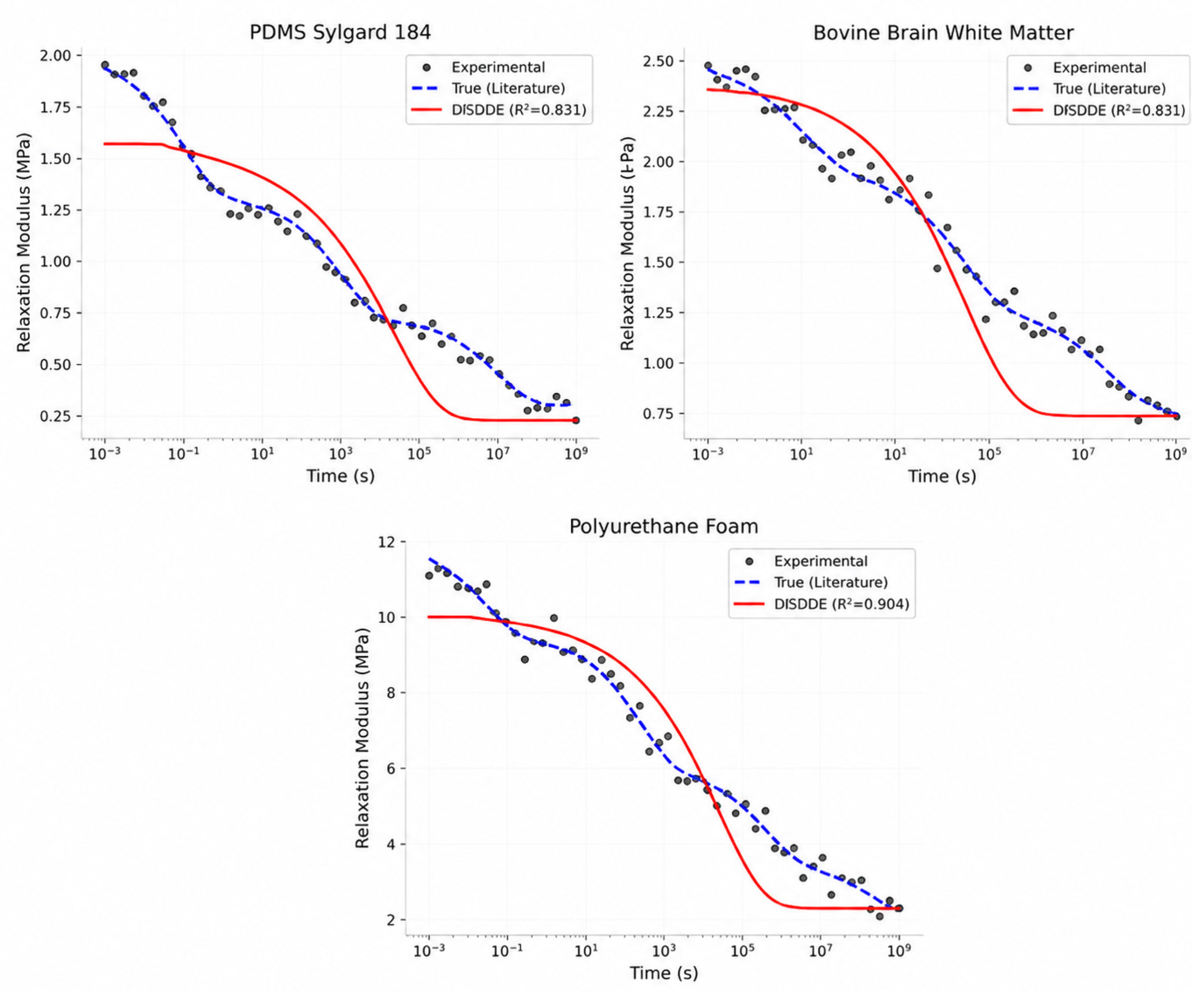
As shown by Figure 1, the model was able to provide an accurate fit to the measured modulus values (red solid lines) and compare these to the measured modulus values (blue circles). Literature-based reference curves have also been added (blue dashed lines) to demonstrate the validity of both the data and the model.

The overall results suggest that the DRSDDE model can capture the behavior of the multi-scaled relaxation in a variety of material systems exhibiting differing levels of mechanical properties and time scales. Most specifically, it has been shown to be capable of predicting both the very fast decay seen early on (short term) as well as the longer-term relaxation trend (long term), characteristics associated with highly complex viscoelastic systems. A very good fit to the measured modulus-time behavior was found for PDMS Sylgard 184. The model does capture the progressive reduction in the modulus by many orders of magnitude as time increases, but there were some small discrepancies in the intermediate time period. There was also an analogous trend found in bovine brain white matter. It appears that this model can accurately represent the slow time-scale relaxation processes typical of soft biological tissues.

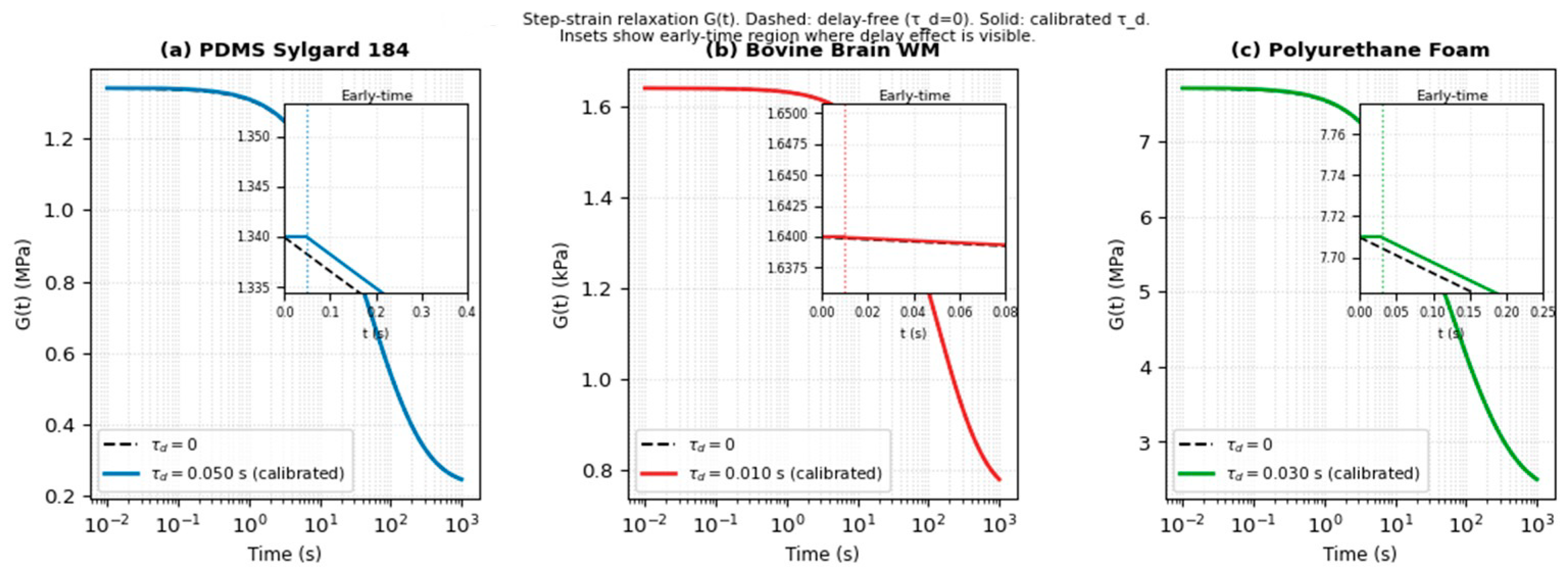
Visual inspection of Figure 1 indicates that the largest discrepancies occur primarily in the intermediate relaxation regime, where the experimental response exhibits local variations that cannot be fully represented by a single Gaussian relaxation spectrum. Nevertheless, the overall decay trend and long-term relaxation behavior are captured accurately. The fit between the model and experimentally determined behavior for polyurethane foam was quite close. This indicates that the distributed relaxation spectrum model has been shown to be particularly effective at capturing non-linear relaxation behaviors common to many types of viscoelastic. The step-strain response of the DRSDDE model is illustrated in Figure 2 for the calibrated materials. The comparison between the delay-free case (${\tau }_d$ = 0) and the fitted delay values demonstrates the influence of finite response time on the relaxation behavior.

The time-dependent effects are most apparent at low time scales where the model’s response to strain is greatly influenced by the delay parameter. The delay parameter shifts the beginning of the relaxation process slightly for short time scales $t < {\tau }_d$. At these time scales, the elastic modulus remains near the instantaneous value of $E_0$. After the transient period $t>{\tau }_d$, the relaxation curves have similar long-time behavior characterized by $E_{\infty }$. Thus, the long-time behavior of the model is unaffected by the presence of the delay parameter. These results confirm that the delay term provides a physically meaningful correction to early-time dynamics without affecting the global relaxation structure.

5.6. Model Performance Comparison

Table 2. Model performance comparison ($R^2$ values).

Material	DRSDDE	Zener	$\mathbf{\Delta }{\mathit{R}}^2$
PDMS Sylgard 184	0.837	0.562	+0.275 (DRSDDE better)
Bovine Brain White Matter	0.831	0.908	−0.077 (Zener better)
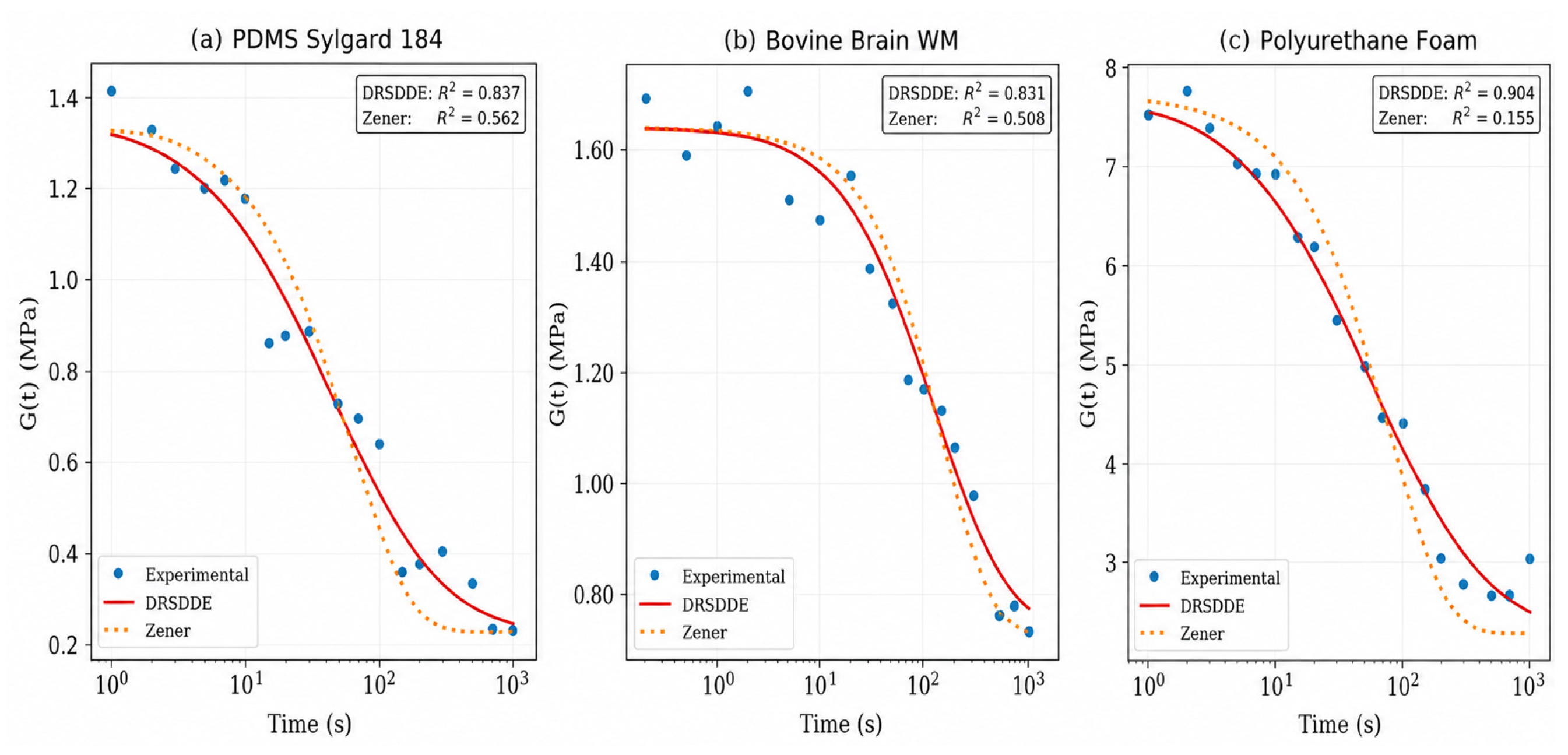
Polyurethane Foam	0.904	0.155	+0.749 (DRSDDE better)

is an analysis of the coefficient of determination ($R^2$) comparing the proposed DRSDDE model with the traditional Zener model. Data show that the DRSDDE model performed better than the Zener model in modeling the complex and multiple length scale relaxations observed in materials like PDMS Sylgard 184 and polyurethane foam.

In comparison to the white matter of the bovine brain, the Zener model has an $R^2$ value that is larger, indicating that for white matter where there is less variation in how quickly it relaxes (i.e., more uniformly), simpler viscoelastic formulations could likely provide satisfactory results. The above example also illustrates that one advantage of the distributed relaxation spectrum model is that as the range of times over which material relaxation occurs becomes wider, the benefits of using a distributed relaxation spectrum model are realized.

Figure 3 highlights the comparison between the proposed DRSDDE model and the classic Zener model with the experimental stress relaxation data. The results clearly show that there are major differences in the ability of each model to describe the experimental data.

The DRSDDE model is much better than the Zener model for PDMS Sylgard 184 and polyurethane foam. The DRSDDE model fits all of the data in this study very well over the whole time range, providing an accurate description of the initial decay as well as the long-term relaxation. The Zener model has very little flexibility and deviates from experimental data, especially at longer timescales. The two models are in good agreement with each other on the white matter from bovine brains. However, the Zener Model appears to have a better fit than the Maxwell Model. This is consistent with the idea that for materials which relax uniformly (i.e., they all relax at the same time), a simpler viscoelastic model will be adequate. These studies collectively indicate that although classical viscoelastic models like the Zener model, etc., can satisfactorily predict simple viscoelastic relaxation processes, this new distributed relaxation spectrum model can accommodate complex, multi-scale relaxation behaviors in materials far better.

5.7. Weight Function Analysis

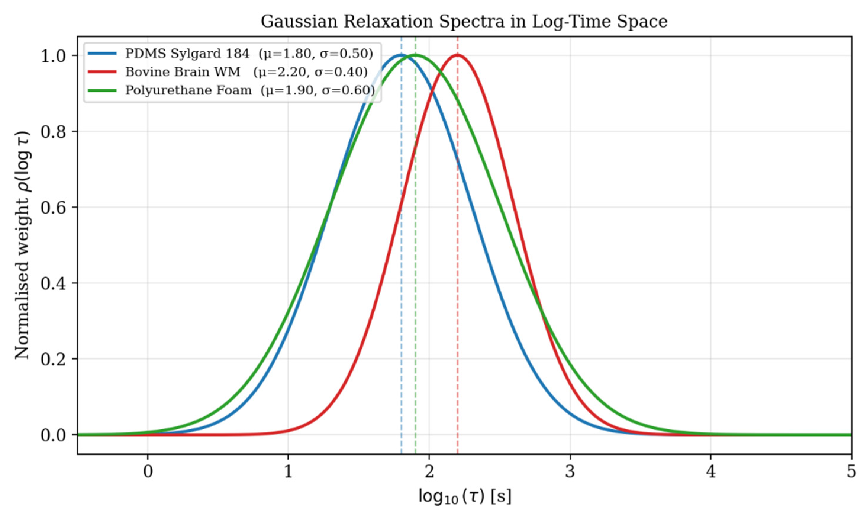
The data provided by the curves from the Gaussian weight function (as depicted in Figure 4) demonstrate how various mechanisms for relaxation are distributed throughout the logarithmic time scale. Each of these curves indicates the total amount of contributions made toward relaxation at each point along the given time scales, which have been defined using both the average $\mu$ and standard deviation $\sigma$ of the parameters.

Each distribution’s maximum represents the major relaxation timescale. The bovine brain white matter has the largest $\mu$; therefore, it is primarily relaxing on the longest timescales. Conversely, the lower $\mu$ values for PDMS Sylgard 184 and polyurethane foam indicate they relax faster. The spread parameter ($\sigma$) determines the extent of the relaxation distribution. The greatest distribution is shown by polyurethane foam; this suggests that many different relaxation processes interact with one another at various time scales. On the other hand, the narrower distribution of brain tissue shows that the relaxation process occurs for a shorter time. The overall evidence is that a unimodal (one-peaked) Gaussian distribution was seen in each material. The results support the use of the distributed relaxation spectrum formulation to describe the relaxation behavior and confirm that the DRSDDE Model captured both the major mode of relaxation and the variability at longer timescales.

5.8. Frequency-Domain Response Analysis

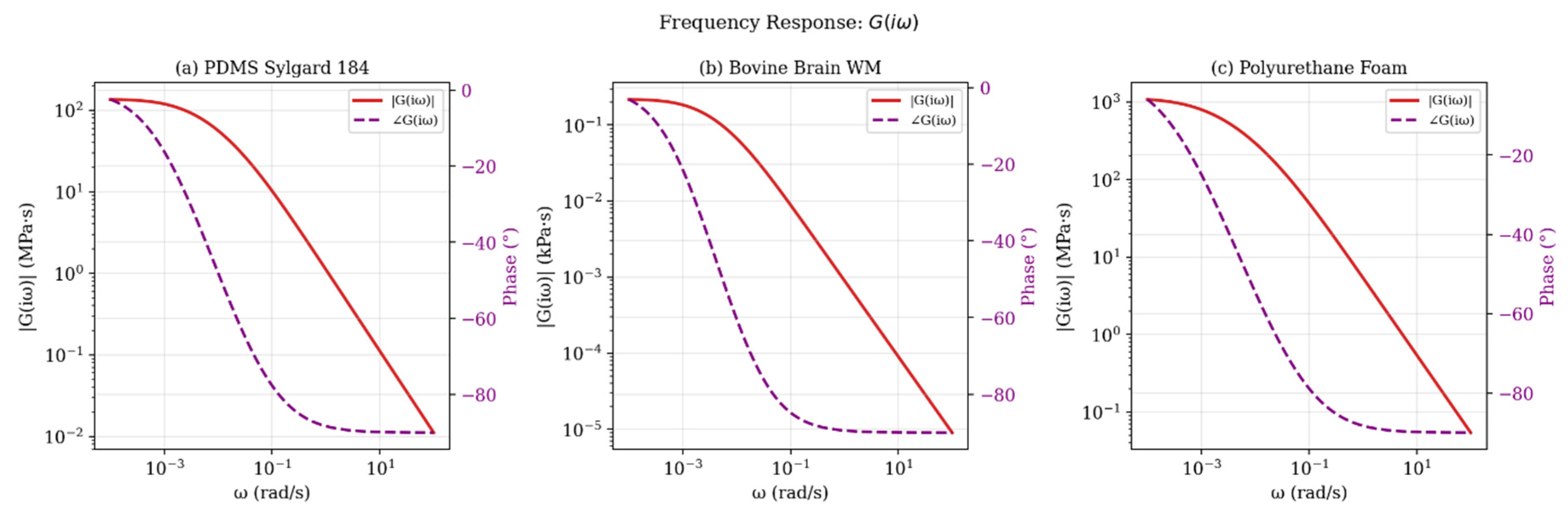
To further evaluate the dynamic behavior of the proposed model, the frequency response function $G\left(i\omega \right)$ is analyzed for the considered materials. Figure 5 illustrates both the magnitude $\mid G\left(i\omega \right)\mid$ and phase $\mathrm{\angle }G\left(i\omega \right)$ as functions of angular frequency $\omega$.

At low frequencies ($\omega \to 0$), the magnitude remains approximately constant, indicating that the materials behave predominantly as elastic solids. This corresponds to the long-term modulus $E_{\mathrm{\infty }}$. As the frequency increases, the magnitude decreases smoothly, reflecting the progressive activation of relaxation mechanisms and the transition toward viscous behavior. The phase response further confirms this transition. At low frequencies, the phase angle is close to zero, indicating elastic-dominated behavior. As $\omega$ increases, the phase decreases toward negative values, approaching a viscous-dominated regime. The smooth variation of the phase angle demonstrates the continuous distribution of relaxation times captured by the DRSDDE model. Differences between materials are also evident. Polyurethane foam exhibits a broader transition region, consistent with its wider relaxation spectrum (larger $\sigma$), while bovine brain tissue shows a sharper transition due to its narrower distribution. PDMS Sylgard 184 demonstrates intermediate behavior between these two extremes. Overall, the frequency-domain analysis confirms that the proposed model captures both the amplitude and phase characteristics of viscoelastic materials across a wide range of frequencies, providing further validation of the distributed relaxation spectrum Gaussian formulation.

5.9. Stability Analysis

The stability of the DRSDDE feedback system $\epsilon \left(t\right)=k \sigma \left(t\right)$ is characterized using the dimensionless normalized loop gain shown below:

$$\tilde{K}={\displaystyle \frac{k G\left(0\right)}{{\tau }_c}}, {\tau }_c={10}^{\mu }.$$

According to Theorem 2, the delay-free system is asymptotically stable if and only if $\tilde{K}<1$. Moreover, a stronger result holds for the considered model class.

Proposition 1.

(Delay-Immune Stability). If  $\tilde{K}<1$, then the system remains asymptotically stable for all delays $\tau \ge 0$.

This follows from the property $\mid G\left(i\omega \right)\mid \le G\left(0\right)$ for all $\omega >0$, which prevents the Hopf condition $k\mid G\left(i\omega \right)\mid =1$ from being satisfied when $kG\left(0\right)<{\tau }_c$. Consequently, no eigenvalues cross the imaginary axis, and stability is preserved independently of the delay.

Table 3. Stability analysis ($k=1/E_0$, $\tilde{K}=kG(0)/{\tau }_c$).

Material	$\mathbf{G}\left(0\right)(\mathbf{M}\mathbf{P}\mathbf{a}·\mathbf{s})$	${\mathit{\tau }}_{\mathit{c}}$ (s)	k = 1/E0 (MPa−1)	$\tilde{\mathrm{K}}$	Stable at τ = 0	Stable at All τ
PDMS Sylgard 184	135.6	63.1	0.7463	1.604	NO	NO
Bovine Brain White Matter	0.218	158.5	609.8	0.838	YES	YES
Polyurethane Foam	1113	79.4	0.1297	1.818	NO	NO

summarizes the stability characteristics for the considered materials, where the feedback gain is taken as $k={\displaystyle \frac{1}{E_0}}$.

The results clearly demonstrate distinct stability regimes across materials. Bovine brain white matter satisfies $\tilde{K}=0.838<1$, and is therefore unconditionally stable for all delay values according to the delay-immune stability proposition. In contrast, PDMS Sylgard 184 and polyurethane foam yield $\tilde{K}>1$, indicating instability in the delay-free case and the potential for delay-induced oscillatory behavior. For these materials, the critical feedback gain is given by

$$k_c={\displaystyle \frac{{\tau }_c}{G\left(0\right)}},$$

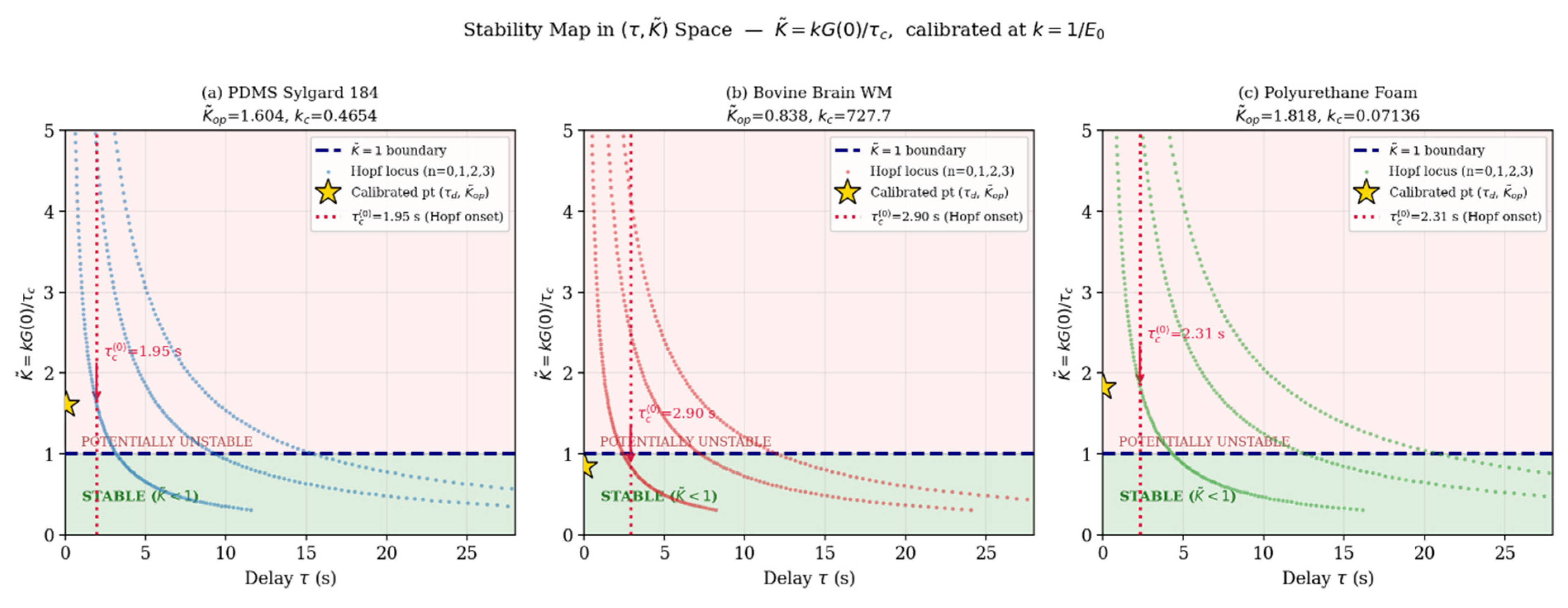
resulting in $k_c=0.465 {\mathrm{MPa}}^{-1}$ for PDMS and $k_c=0.071 {\mathrm{MPa}}^{-1}$ for polyurethane foam. The calibrated gains $k={\displaystyle \frac{1}{E_0}}$ exceed these thresholds, confirming that the systems operate in a regime where instability may arise. Figure 6 presents the stability maps in the $\left(\tau ,\tilde{K}\right)$ parameter space. The horizontal line $\tilde{K}=1$ defines the delay-free stability threshold, while the Hopf loci indicate delay-induced instability boundaries. For materials with $\tilde{K}>1$ (PDMS and polyurethane foam), the system may undergo Hopf bifurcation beyond critical delay values, leading to oscillatory instabilities. In contrast, bovine brain white matter satisfies $\tilde{K}<1$, and no Hopf crossings occur within the physically admissible regime, confirming delay-independent stability.

5.10. Hopf Bifurcation Analysis

To quantitatively characterize the delay-induced instability boundaries identified in Figure 5, we compute the Hopf bifurcation conditions for materials with normalized loop gain $\tilde{K}>1$. These bifurcations correspond to the emergence of oscillatory solutions when a pair of complex conjugate characteristic roots crosses the imaginary axis. The Hopf condition is obtained from the characteristic equation of the form $F\left(s\right)=1-k{e}^{-i\omega \tau }G\left(i\omega \right).$ Referring to Equation (6) and Theorem 3, and using the calibrated parameters and Gauss–Legendre quadrature for numerical evaluation, the critical frequencies and delays are computed and summarized in

Table 4. Hopf bifurcation parameters (with $k=1/E_0$).

Material	$\tilde{\mathit{K}}$	${\mathit{\omega }}_{\mathit{c}}(\mathbf{r}\mathbf{a}\mathbf{d}/\mathbf{s})$	${\mathit{\tau }}_{\mathit{c}}^{\left(0\right)}$	${\mathit{\tau }}_{\mathit{c}}^{\left(1\right)}$	${\mathit{\tau }}_{\mathit{c}}^{\left(2\right)}$	${\mathit{T}}_{\mathit{c}}=\frac{2\mathit{\pi }}{{\mathit{\omega }}_{\mathit{c}}}$	$\frac{{\mathit{\tau }}_{\mathit{d}}}{{\mathit{\tau }}_{\mathit{c}}^{\left(0\right)}}$
PDMS Sylgard 184	1.604	0.8254	1.947	5.753	9.559	7.612	0.026
Bovine Brain White Matter	0.838	-	-	-	-	-	-
Polyurethane Foam	1.818	0.6979	2.312	6.813	11.314	9.003	0.013

.

The results show that Hopf bifurcations occur only for materials with $\tilde{K}>1$, namely PDMS Sylgard 184 and polyurethane foam. The corresponding critical frequencies lie in the range ${\omega }_c\approx 0.70–0.83$ rad/s, which corresponds to oscillation periods $T_c\approx 7.6–9.0$ s. These values indicate that any instability would manifest as low-frequency oscillatory behavior. In contrast, bovine brain white matter satisfies $\tilde{K}<1$, and therefore no Hopf bifurcation occurs for any $\tau \ge 0$. This confirms the delay-independent stability condition established in Section 4. A key observation is that the calibrated delay values (${\tau }_d=0.03–0.05$) are significantly smaller than the first critical Hopf delay ${\tau }_c^{\left(0\right)}$. Specifically, the ratio ${\tau }_d/{\tau }_c^{\left(0\right)}$ lies between 0.013 and 0.026, indicating that the system operates far from the instability threshold. Consequently, the fitted models remain well within the stable regime, and the observed viscoelastic responses are governed by intrinsic relaxation dynamics rather than delay-induced oscillations. Note that the calibrated delay values are relatively small, ranging from 0.01 s to 0.05 s for the materials considered in this study. These values are several orders of magnitude smaller than the dominant relaxation times associated with the distributed relaxation spectrum. Consequently, the delay term should not be interpreted as a direct macroscopic wave propagation or transport time. Instead, it represents an effective phenomenological parameter that accounts for unresolved internal processes, including microstructural rearrangements, delayed stress transfer mechanisms, and possible experimental or loading-system latencies. Within the proposed framework, the delay parameter provides additional flexibility for capturing short-time transient effects while remaining sufficiently small to preserve the overall stability of the calibrated models.

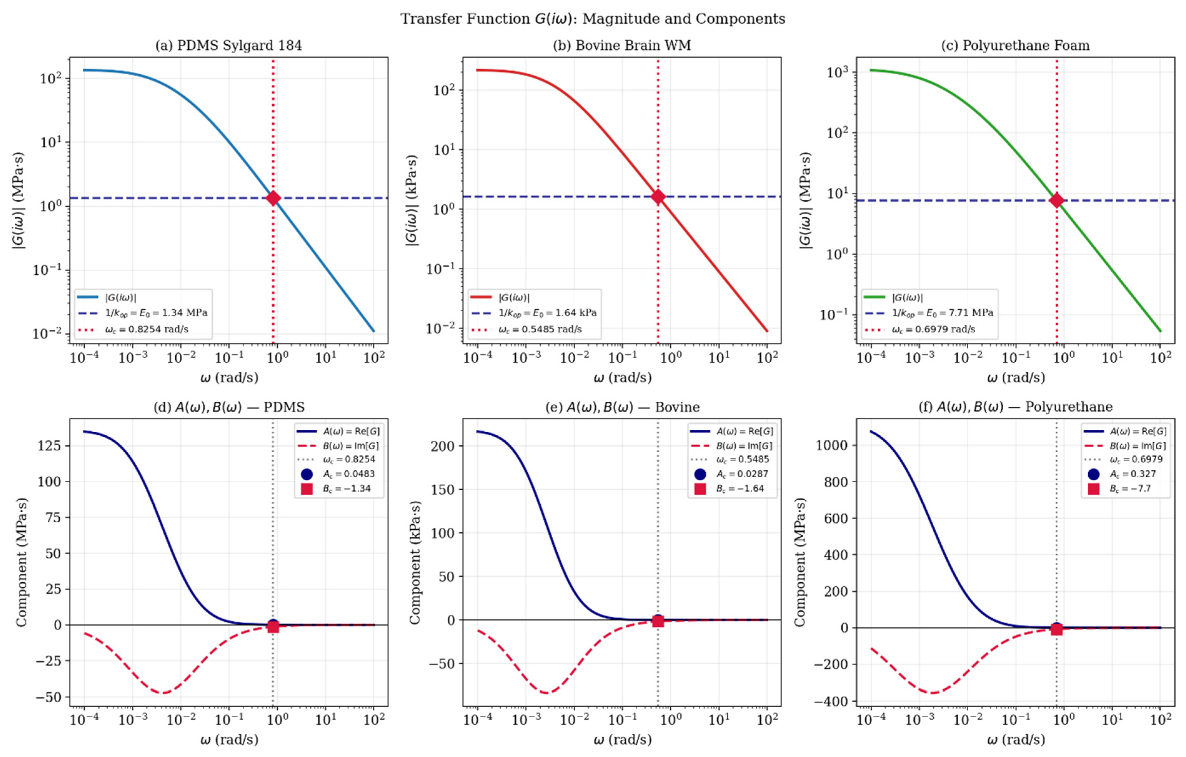
Finally, as illustrated in Figure 5, the Hopf bifurcation loci define the boundary of the potentially unstable region in the $\left(\tau ,\tilde{K}\right)$ parameter space. As the feedback gain approaches the critical value $k_c={\tau }_c/G\left(0\right)$, the stability margin decreases rapidly, highlighting the sensitivity of the system to parameter variations near the bifurcation threshold. To validate the Hopf bifurcation condition derived in Section 4, the frequency-domain response of the system is analyzed. Figure 7 shows the magnitude of the transfer function $\mid G\left(i\omega \right)\mid$ together with the threshold $1/k$. The intersection point determines the critical frequency ${\omega }_c$, satisfying the condition $k\mid G\left(i{\omega }_c\right)\mid =1$.

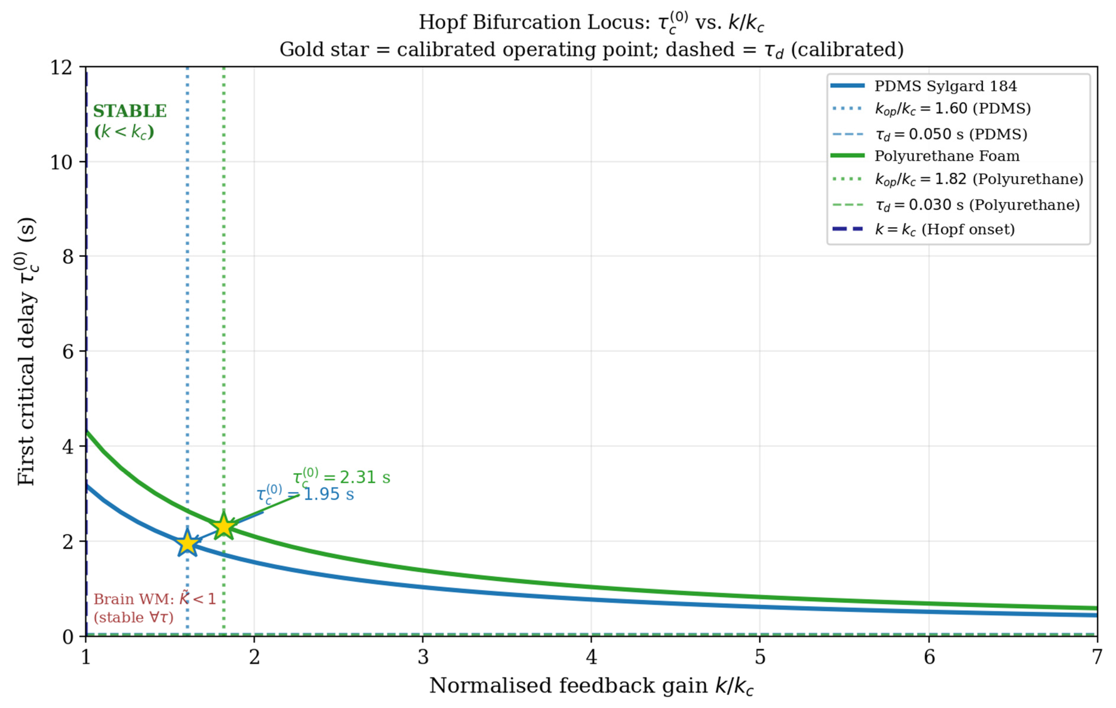
The lower panels display the real and imaginary components $A\left(\omega \right)$ and $B\left(\omega \right)$, which are used to compute the critical delay values via the phase condition. For PDMS Sylgard 184 and polyurethane foam, a clear intersection is observed, confirming the existence of a Hopf bifurcation. In contrast, for bovine brain white matter, no intersection occurs within the admissible frequency range, consistent with the condition $\tilde{K}<1$ and the absence of bifurcation. The Hopf bifurcation structure of the DRSDDE model is illustrated in Figure 8, where the first critical delay ${\tau }_c^{\left(0\right)}$ is plotted as a function of the normalized feedback gain $k/k_c$. The bifurcation boundary originates at $k/k_c=1$, corresponding to the critical gain at which oscillatory instability first emerges.

It is observed that the critical delay decreases monotonically as the feedback gain increases, indicating that systems with stronger feedback become more sensitive to delay-induced instability. This behavior is consistent with the analytical condition $k\mid G\left(i{\omega }_c\right)\mid =1$. Markers indicate the calibrated operating points for PDMS Sylgard 184 and polyurethane foam. In both cases, the identified delay values ${\tau }_d$ are significantly smaller than the corresponding critical delays ${\tau }_c^{\left(0\right)}$, confirming that the system operates well within the stable regime. The Hopf bifurcation structure of the DRSDDE model is illustrated in Figure 8, where the first critical delay ${\tau }_c^{\left(0\right)}$ is plotted as a function of the normalized feedback gain $k/k_c$. The bifurcation boundary originates at $k/k_c=1$, corresponding to the critical gain at which oscillatory instability first emerges. It is observed that the critical delay decreases monotonically as the feedback gain increases, indicating that systems with stronger feedback become more sensitive to delay-induced instability. This behavior is consistent with the analytical condition $k\mid G\left(i{\omega }_c\right)\mid =1$. The calibrated operating points for PDMS Sylgard 184 and polyurethane foam are indicated by markers. In both cases, the identified delay values ${\tau }_d$ are significantly smaller than the corresponding critical delays ${\tau }_c^{\left(0\right)}$, confirming that the system operates well within the stable regime.

6. Conclusions

The researchers have created a Distributed Relaxation Spectrum Delay Differential Equation (DRSDDE) modeling method to describe the viscoelastic properties of materials with multiple scales of relaxation behavior and also include finite-time responses. This new approach incorporates a Gaussian distribution of relaxation times on a logarithmic time scale, as well as uses Legendre-Gauss Quadrature to numerically evaluate the DRSDDE. The result is an easily interpreted and very flexible description of material behavior, which can be used to model viscoelastic behaviors that go beyond those described by models based upon a single relaxation time.

The validation of the model used three different experimental sets of data: PDMS Sylgard 184, bovine brain white matter, and polyurethane foam. The results show that the DRSDDE model is in good agreement with the experiments and has a coefficient of determination ($R^2$) of 0.837, 0.831, and 0.904 for each set of data. Most importantly, the DRSDDE model shows better performance than the classic Zener model when dealing with materials having large relaxation spectra; this result demonstrates the ability of the DRSDDE model to represent material properties over multiple length scales and complex viscoelastic behavior. The parameters also provide useful information on the nature of the materials tested as they are related to physical timescales of relaxation ($\mu$) and to the distribution widths of the relaxation mechanisms ($\sigma$).

From a theoretical perspective, the stability and bifurcation structure of the model were rigorously analyzed through the characteristic equation. A key result of this work is the establishment of the Delay-Immune Stability Proposition, which states that systems with normalized gain $\tilde{K} < 1$ are asymptotically stable for all delay values. This condition is satisfied for bovine brain white matter ($\tilde{K} = 0.838$), confirming unconditional stability. For PDMS Sylgard 184 and polyurethane foam ($\tilde{K} > 1$ under calibrated parameters), Hopf bifurcation analysis reveals the existence of critical delay thresholds, with first bifurcation points at ${\tau }_c^{\left(0\right)} \approx 1.95$ s and 2.31 s, respectively, corresponding to oscillation periods of approximately 7.6 s and 9.0 s. Importantly, the calibrated delay values are significantly smaller—by factors of 40–75—than these critical thresholds, indicating that all fitted models operate well within the stable regime.

In general, the proposed DRSDDE model is an efficient model to describe viscoelastic behaviors in materials that present complex relaxation features, as it combines high prediction quality (accuracy) with a very strong scientific basis. The obtained results have demonstrated that the incorporation of Distributed Relaxation Spectrum Dynamics (DRSD) and Delays (DE) has enhanced both the precision of the models and the understanding of how materials react under different conditions.

Future work will be focused on extending this framework by including both temperature-dependent and frequency-domain effects. In addition, there is potential for a more complete nonlinear bifurcation analysis in addition to experimental validation of those oscillation regimes that are predicted under critical parameters.

References

1. Kelvin, W.T. On the Elasticity and Viscosity of Metals. Proc. R. Soc. Lond. 1865, 14, 289–297. [Google Scholar] [CrossRef]
2. Voigt, W. Über die Beziehung zwischen den beiden Elasticitätsconstanten isotroper Körper. Ann. Phys. 1889, 274, 573–587. [Google Scholar] [CrossRef]
3. Zener, C. Elasticity and Anelasticity of Metals; University of Chicago Press: Chicago, IL, USA, 1965. [Google Scholar]
4. Eldred, L.B.; Baker, W.P.; Palazotto, A.N. Kelvin-Voigt versus fractional derivative model as constitutive relations for viscoelastic materials. AIAA J. 1995, 33, 547–550. [Google Scholar] [CrossRef] [PubMed]
5. Caputo, M. Linear models of dissipation whose Q is almost frequency independent—II. Geophys. J. Int. 1967, 13, 529–539. [Google Scholar] [CrossRef]
6. Caputo, M.; Mainardi, F. A new dissipation model based on a memory mechanism. Pure Appl. Geophys. 1971, 91, 134–147. [Google Scholar] [CrossRef]
7. Bagley, R.L.; Torvik, P.J. Fractional calculus in the transient analysis of viscoelastically damped structures. AIAA J. 1985, 23, 918–925. [Google Scholar] [CrossRef] [PubMed]
8. Podlubny, I. Fractional Differential Equations: An Introduction to Fractional Derivatives, Fractional Differential Equations, to Methods of Their Solution and Some of Their Applications; Elsevier: Amsterdam, The Netherlands, 1998; Volume 198. [Google Scholar]
9. Mainardi, F.; Spada, G. Creep, relaxation and viscosity properties for basic fractional models in rheology. Eur. Phys. J. Spec. Top. 2011, 193, 133–160. [Google Scholar] [CrossRef]
10. Rossikhin, Y.A.; Shitikova, M.V. Application of fractional calculus for dynamic problems of solid mechanics: Novel trends and recent results. Appl. Mech. Rev. 2010, 63, 010801. [Google Scholar] [CrossRef]
11. Mainardi, F. Fractional Calculus and Waves in Linear Viscoelasticity: An Introduction to Mathematical Models; World Scientific: Singapore, 2022. [Google Scholar]
12. Caputo, M. Distributed Order differential equations modelling dielectric induction and diffusion. Fract. Calc. Appl. Anal. 2001, 4, 421–442. [Google Scholar]
13. Chechkin, A.V.; Gorenflo, R.; Sokolov, I.M. Retarding subdiffusion and accelerating superdiffusion governed by Distributed Relaxation Spectrum fractional diffusion equations. Phys. Rev. E 2002, 66, 046129. [Google Scholar] [CrossRef]
14. Atanackovic, T.M.; Pilipovic, S.; Stankovic, B.; Zorica, D. Fractional Calculus with Applications in Mechanics: Vibrations and Diffusion Processes; John Wiley & Sons: Hoboken, NJ, USA, 2014. [Google Scholar]
15. Giusti, A.; Colombaro, I.; Garra, R.; Garrappa, R.; Mentrelli, A. On variable-order fractional linear viscoelasticity. Fract. Calc. Appl. Anal. 2024, 27, 1564–1578. [Google Scholar] [CrossRef]
16. Hale, J.K.; Lunel, S.M.V. Introduction to Functional Differential Equations; Springer Science & Business Media: Berlin/Heidelberg, Germany, 2013; Volume 99. [Google Scholar]
17. Erneux, T. Applied Delay Differential Equations; Springer: Berlin/Heidelberg, Germany, 2009. [Google Scholar]
18. Niculescu, S.I. Delay Effects on Stability: A Robust Control Approach; Springer: London, UK, 2002. [Google Scholar]
19. Gu, K.; Chen, J.; Kharitonov, V.L. Stability of Time-Delay Systems; Springer Science & Business Media: Berlin/Heidelberg, Germany, 2003. [Google Scholar]
20. Michiels, W.; Niculescu, S.I. Stability and Stabilization of Time-Delay Systems: An Eigenvalue-Based Approach; Society for Industrial and Applied Mathematics: Philadelphia, PA, USA, 2007. [Google Scholar]
21. Sipahi, R.; Niculescu, S.I.; Abdallah, C.T.; Michiels, W.; Gu, K. Stability and stabilization of systems with time delay. IEEE Control Syst. Mag. 2011, 31, 38–65. [Google Scholar]
22. Christensen, R.M. Theory of Viscoelasticity; Courier Corporation: North Chelmsford, MA, USA, 2013. [Google Scholar]
23. Lakes, R.S. Viscoelastic Solids (1998); CRC Press: Boca Raton, FL, USA, 2017. [Google Scholar]
24. Varner, H.; Cohen, T. Explaining the spread in measurement of PDMS elastic properties: Influence of test method and curing protocol. Soft Matter 2024, 20, 9174–9183. [Google Scholar] [CrossRef] [PubMed]
25. Budday, S.; Nay, R.; De Rooij, R.; Steinmann, P.; Wyrobek, T.; Ovaert, T.C.; Kuhl, E. Mechanical properties of gray and white matter brain tissue by indentation. J. Mech. Behav. Biomed. Mater. 2015, 46, 318–330. [Google Scholar] [CrossRef] [PubMed]
26. Zielonka, P.; Junik, K.; Duda, S.; Socha, T.; Kula, K.; Denisiewicz, A.; Olaleye, K.; Macek, W.; Lesiuk, G.; Błażejewski, W. Stress relaxation behaviour modeling in rigid polyurethane (PU) elastomeric materials. Materials 2023, 16, 3156. [Google Scholar] [CrossRef] [PubMed]
Figure 1. Stress relaxation modulus for PDMS Sylgard 184, Bovine Brain White Matter, and Polyurethane Foam. Experimental data (circles), true literature values (dashed blue), and DRSDDE model fits (solid red).
Applsci 16 05955 g001
Figure 2. Step-strain relaxation response of the DRSDDE model for the considered materials.
Applsci 16 05955 g002
Figure 3. Model comparison showing DRSDDE (red) and Zener (dotted) model fits to experimental data (circles).
Applsci 16 05955 g003
Figure 4. Gaussian relaxation weight functions ρ ( l o g   τ ) in logarithmic time-scale space for the considered materials. The vertical dashed lines indicate the mean values μ of the corresponding Gaussian distributions, representing the dominant relaxation time scales in log-time coordinates.
Applsci 16 05955 g004
Figure 5. Frequency response of the DRSDDE model for different materials: (a) PDMS Sylgard 184, (b) bovine brain white matter, and (c) polyurethane foam.
Applsci 16 05955 g005
Figure 6. Stability regions in the τ K ~ parameter space for (a) PDMS Sylgard 184, (b) bovine brain white matter, and (c) polyurethane foam. The colored solid and dotted curves represent Hopf bifurcation boundaries obtained from the characteristic equation of the proposed model. The horizontal blue dashed line corresponds to the critical normalized gain value equal to one, which separates the delay-immune stable regime (normalized gain less than one) from the region where delay-induced instability may occur (normalized gain greater than one). The yellow star indicates the calibrated operating point determined from the fitted material parameters and calibrated delay value. The vertical red dotted line denotes the first critical Hopf delay at which purely imaginary characteristic roots appear. The red arrow highlights the location of this first critical delay. The green region corresponds to parameter combinations predicted to be stable, whereas the shaded red region represents parameter combinations for which delay-induced instability may occur.
Applsci 16 05955 g006
Figure 7. Frequency-domain validation of the Hopf bifurcation condition. The top row shows the magnitude of the transfer function | G ( i ω ) | for PDMS Sylgard 184, bovine brain white matter, and polyurethane foam. The horizontal dashed line represents the critical value 1 / k , while the vertical dotted line indicates the critical frequency ωc at which the Hopf condition | G ( i ω c ) |   =   1 / k is satisfied. The diamond marker denotes the intersection corresponding to the critical frequency. The bottom row shows the real component A ( ω ) and imaginary component B ( ω ) of the transfer function. The blue circular marker indicates the critical value A c   =   A ( ω c ) , and the red square marker indicates the critical value B c   =   B ( ω c ) evaluated at the critical frequency ωc.
Applsci 16 05955 g007
Figure 8. Hopf bifurcation locus showing the first critical delay τ c 0 as a function of normalized feedback gain k / k c for PDMS Sylgard 184 and polyurethane foam. The gold star denotes the calibrated operating point obtained from the identified material parameters.
Applsci 16 05955 g008