How Could Supercontinent Cycle Modulate the Periodicity and Phase of Global Plume Heat Flux?

Abstract

Supercontinent cycles are fundamental processes driving the tectonic evolution of Earth, and the periodic assembly and breakup of supercontinents may exert significant influence on global plume heat flux. Large igneous province (LIP) events provide a geological record of mantle plume activity, and their periodicity shows a striking correspondence with the periodicity of supercontinent cycles, suggesting a potential coupling between supercontinent cycles and plume activity. In this study, we employ two-dimensional spherical shell simulations using ASPECT to model the evolution of global plume heat flux, with a focus on its periodicity and phase, which are then compared with the observed periodicity and phase of LIP events. Given the uncertainties in the mode and period of supercontinent cycles, and the potentially important role of the compositionally anomalous and intrinsically dense (CAID) layer, we incorporate all three factors into our models. We then explore the conditions under which the periodicity of global plume heat flux matches the periodicity of supercontinent cycles. We find that the cycle period is the dominant control on the periodicity of global plume heat flux, while the cycle mode significantly modulates its phase. These results suggest that supercontinent cycles regulate not only the periodicity of mantle plume activity but also the timing of heat flux variations.

1. Introduction

The periodic assembly and breakup of supercontinents, together forming the supercontinent cycle, are fundamental tectonic events in Earth’s history. The supercontinent cycle has been operating for at least ~2.5 Ga [1], with individual cycle timescales of approximately 400–800 Myr [2,3,4,5]. The supercontinent cycle reflects global plate tectonics and mantle convection [6,7,8], deeply influencing the evolution of Earth’s systems and also profoundly influencing climate and life [9,10,11,12,13]. The supercontinent cycle involves multiple modes [14,15]. The introversion mode involves the closure of the interior ocean inherited from the breakup of the supercontinent, whereas the extroversion mode closes the exterior ocean that surrounded the supercontinent [1,6,7,8]. The combination mode involves closure of both interior and exterior oceans [16]. Mitchell et al. [17] have proposed that a supercontinent can form at a position rotated 90° from the previous one—a model termed orthoversion. Yoshida [14] considered that this orthoversion model can be classified as a kind of combination mode. These three modes control the spatial distribution of subduction zones, thereby potentially exerting distinct influences on deep mantle structure [18].

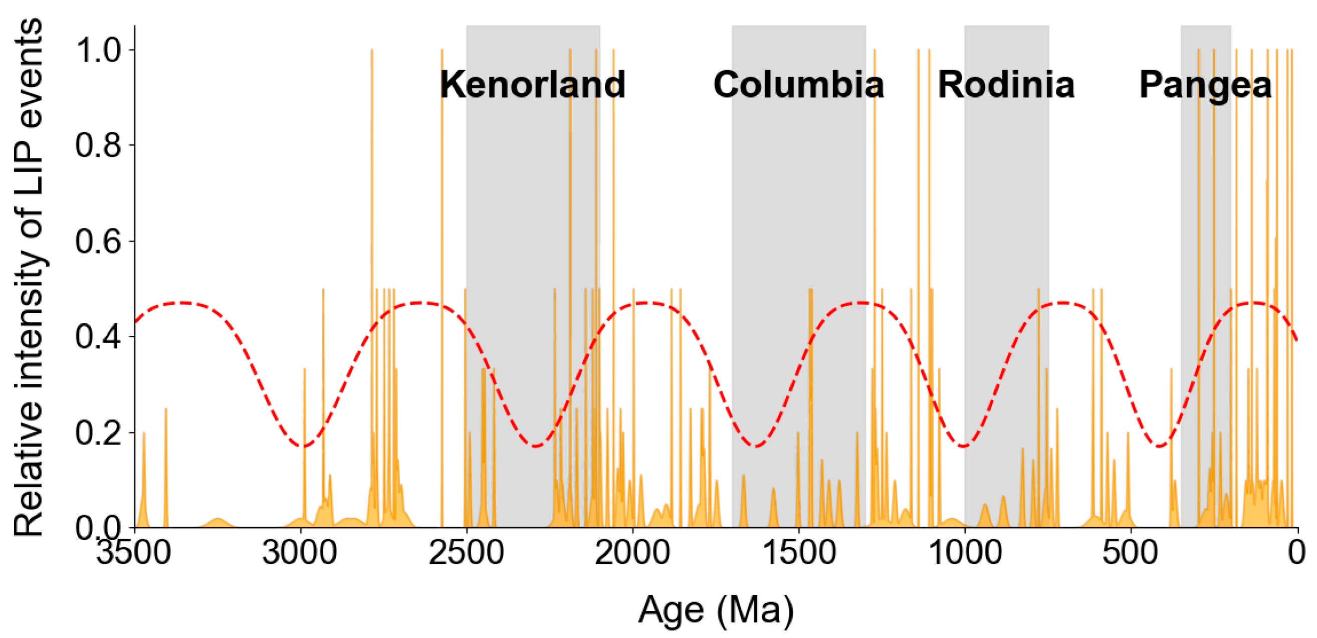
Large igneous province (LIP) events exhibit a periodicity that matches the periodicity of the supercontinent cycle [5,19] (Figure 1). These observations suggest that supercontinent cycles may play a key role in regulating both the periodicity and phase of global plume heat flux. However, existing studies on the relationship between supercontinent cycles and mantle plumes have only focused on a single supercontinent mode or localized simulations, lacking a systematic comparison of global plume heat flux evolution across different supercontinent cycle modes [18,20,21].

Furthermore, the thermochemical structure of the deep mantle may influence plume activity. At the base of the lower mantle, large low sear velocity provinces (LLSVPs) are widely regarded as primary source regions for mantle plumes [22] and may interact profoundly with surface tectonic processes through mantle convection [23]. Although the nature of LLSVPs remains debated, they are commonly interpreted as thermally or chemically heterogeneous mantle material [24,25,26]. In numerical models, such heterogeneity can be represented by a CAID mantle component, which we include in our simulations [27].

Figure 1. Relative intensity curve (orange fill) of LIP events since 3500 Ma [28], with supercontinent assembly periods shown as gray shaded areas: Kenorland (~2500–2100 Ma), Columbia (~1700–1300 Ma), Rodinia (~1000–750 Ma), and Pangea (~350–200 Ma). The red dashed line demonstrates the possible cyclic nature of mantle plume activity with ca. 750–550 Myr periodicity [29].

Figure 1. Relative intensity curve (orange fill) of LIP events since 3500 Ma [28], with supercontinent assembly periods shown as gray shaded areas: Kenorland (~2500–2100 Ma), Columbia (~1700–1300 Ma), Rodinia (~1000–750 Ma), and Pangea (~350–200 Ma). The red dashed line demonstrates the possible cyclic nature of mantle plume activity with ca. 750–550 Myr periodicity [29].

In this study, we use two-dimensional spherical shell models with the CAID material to compare global plume heat flux periodicity across three supercontinent cycle modes and address the following three key questions:

• What influences the periodicity of global plume heat flux?
• How do different supercontinent cycle modes affect the phase of global plume heat flux?
• What is the connection between the phase of global plume heat flux and LIP events?

2. Materials and Methods

2.1. Governing Equations

We use the geodynamic simulation software ASPECT 3.0, based on the finite element and particle method, to solve a two-dimensional spherical shell model. This software has been extensively used to model similar problems [20,30,31]. Equations (1)–(4) describe the conservation of mass, momentum, energy, and composition, respectively, for compressible mantle convection.

$$\nabla \cdot \left(\rho \mathit{u}\right)=0$$

(1)

$$-\nabla \cdot \left(2\eta {\dot{\epsilon }}_{II}\right)+\nabla P=\rho \mathit{g}$$

(2)

$$\rho C_p\left({\displaystyle \frac{\mathsf{\partial }T}{\mathsf{\partial }t}}+\mathit{u}\cdot \nabla T\right)-\nabla \cdot \left(k\nabla T\right)=\rho H+2\eta {\dot{\epsilon }}_{II}+\alpha T\left(\mathit{u}\cdot \nabla P\right)$$

(3)

$${\displaystyle \frac{\mathsf{\partial }c}{\mathsf{\partial }t}}+\mathit{u}\cdot \nabla c=0$$

(4)

Here, $\rho$ is density, $\mathit{u}$ velocity, $\eta$ viscosity, ${\dot{\epsilon }}_{II}$ strain rate, $P$ pressure, $\mathit{g}$ gravitational acceleration, $C_p$ specific heat capacity, $T$ temperature, $k$ thermal conductivity, $H$ internal heating rate, $\alpha$ thermal expansivity, and $c$ compositional fields. Detailed parameters for all models are shown in

Table 1. Model global parameters.

Parameter	Symbol	Value
Top boundary temperature	$T_{top}$	300 K
Bottom boundary temperature	$T_{bottom}$	3800 K
Earth core radius	$R_i$	3481 km
Earth radius	$R_o$	6371 km
Gravitational acceleration	$\mathit{g}$	9.81 m s−2
Thermal diffusivity	$k$	1 × 10−6 m2 s−1
Heat capacity	$C_p$	1250 J kg−1 K−1
Radiogenic heat production rate a	$H$	2.09 × 10−12 W kg−1
Mantle reference density	${\rho }_0$	3316 kg m−3
CAID density difference b	$∆{\rho }_c$	150 kg m−3
CAID viscosity difference b	${\eta }_c$	10
Minimum viscosity	${\eta }_{min}$	1 × 1020 Pa s
Maximum viscosity	${\eta }_{max}$	1 × 1025 Pa s
Isothermal compressibility	${\beta }_T$	4 × 10−12 Pa−1
Cohesion	$C$	100 MPa
Friction angle	$\Phi$	0.32

References: a [18], b [32].

.

We use the isentropic compression approximation to handle the compressible equation [30]. Under the isentropic compression approximation, Equation (1) is modified as in Equation (5):

$$\nabla \cdot \mathit{u}=-{\beta }_{\mathrm{T}}\rho \mathit{g}\cdot \mathit{u}$$

(5)

where ${\beta }_{\mathrm{T}}$ is the isothermal compressibility.

The density in our model is related to the temperature, pressure, and compositional fields by Equation (6):

$$\rho (P,T,c)=({\rho }_0+{{\rho }_0\beta }_T(P-P_{adi})+∆{\rho }_{c}c+\mathsf{\Delta }{\rho }_{phase})(1-\alpha (T-T_{adi}\left)\right)$$

(6)

where ${\rho }_0$ is the reference density, $P_{adi}$ the adiabatic pressure, $∆{\rho }_c$ the CAID density difference, $T_{adi}$ the adiabatic temperature, and $\mathsf{\Delta }{\rho }_{phase}$ the density between phase transitions.

The global parameters used in this study are summarized in Table 1.

2.2. Rheological Conditions

Table 2. Model rheology parameters.

Rheology Parameter	Upper Mantle	Mantle Transition		Lower Mantle
Prefactor $A$ (Pa−1 s−1) a	6 × 10−17	7 × 10−17		9 × 10−19
Activation energy $E_a$ (J mol−1) a	150 × 103	150 × 103		150 × 103
Activation volume $V_a$ (m3 mol−1) a	6.34 × 10−7	14.34 × 10−7		10.04 × 10−7
Thermal expansivity coefficients ${\alpha }_0$ (K−1) b	3.15 × 10−5	2.84 × 10−5		2.68 × 10−5
Thermal expansivity coefficients ${\alpha }_1$ (K−2) b	1.02 × 10−8	6.49 × 10−9		4.82 × 10−9
Thermal expansivity coefficients ${\alpha }_2$ (K) b	−0.76	−0.88		−0.93
Thermal expansivity coefficients ${\alpha }_3$ (GPa−1) b	3.63 × 10−2	2.61 × 10−2		2.15 × 10−2
Phase transition depth $D_{trans}\left(\mathrm{k}\mathrm{m}\right)$ c	410		660
Transition temperature $T_{trans}\left(K\right)$ c	1700		1900
Clapeyron slope $\gamma \left({\mathrm{M}\mathrm{P}\mathrm{a}K}^{-1}\right)$ c	3		−2.5
Density difference $\mathsf{\Delta }{\rho }_{trans}\left(\mathrm{k}\mathrm{g}{\mathrm{m}}^{-3}\right)$ c	273		341
Phase transition width $d_w\left(\mathrm{k}\mathrm{m}\right)$ c	50		50

References: a [33], b [34], c [35].

summarizes the rheological parameters used in this study.

To accurately describe the variation of the thermal expansion coefficient with pressure, temperature, and mineral phase, this study directly adopts the parameterization scheme established by Tosi et al. [34], as written in Equation (7):

$$\alpha \left(T,P\right)=\left(a_0+a_{1}T+a_2{T}^{-2}\right)\mathrm{e}\mathrm{x}\mathrm{p}\left(-a_{3}P\right)$$

(7)

where $a_i$ ($i$ = 0, …, 3) are phase-dependent fitting coefficients.

Our rheological formulation is similar to the previous study [33]. The mantle viscosity $\eta$ depends on temperature, pressure and composition, and is defined by Equation (8):

$$\eta \left(P,T\right)=A^{-1}\mathrm{e}\mathrm{x}\mathrm{p}\left[{\displaystyle \frac{E_a+P{V}_a}{RT}}\right]\mathrm{e}\mathrm{x}\mathrm{p}[cln{\eta }_c]$$

(8)

where $A$ is the pre-exponential factor and $E_a$ and $V_{\mathrm{a}}$ are the activation energy and activation volume, respectively. These parameters are all related to the mineral phase. Additionally, ${\eta }_c$ denotes the viscosity coefficient associated with the composition field $c$.

The phase function $\Gamma$ is defined by Equation (9):

$$\Gamma ={\displaystyle \frac{1}{2}}(1+\mathrm{t}\mathrm{a}\mathrm{n}\mathrm{h}({\displaystyle \frac{P-\rho \mathit{g}{D}_{trans}-\gamma (T-T_{trans})}{\rho \mathit{g}{d}_w}}))$$

(9)

where $D_{trans}$ is phase transition depth, $\gamma$ Clapeyron slope, $T_{trans}$ transition temperature, and $d_w$ phase transition width. This study only considers phase transitions at two depths: 410 and 660 km.

Plastic deformation is also considered. A yield stress ${\tau }_y$ and an effective viscosity ${\eta }_{eff}$ are defined by Equations (10) and (11):

$${\tau }_y=Ccos\varphi +Psin\varphi$$

(10)

$${\eta }_{eff}=\mathrm{m}\mathrm{i}\mathrm{n}\left[\eta (P,T),{\displaystyle \frac{{\tau }_y}{2{\dot{\epsilon }}_{II}}}\right]$$

(11)

where $C$ is cohesion, and $\varphi$ is friction angle.

The mantle viscosity parameters are constrained by observations but have relatively large uncertainties. The main features of the viscosity in this study are a 30-fold viscosity jump at 660 km depth and a 10-fold viscosity variation in the lower mantle, which are considered relatively consistent with Earth’s present-day situation in the previous study [35].

The CAID material is modeled using compositional fields. Compared with the background mantle, the compositional field exhibits higher viscosity and density [27]. These properties are specifically controlled through the CAID density difference ($∆{\rho }_c$) and the CAID viscosity difference (${\eta }_c$).

In our model, material properties such as thermal conductivity and compressibility are treated as constants. This simplification was adequate for global-scale problems [27,33].

These parameters ensure that average mantle temperatures evolve in line with Earth’s gradual cooling history and keep the core–mantle boundary (CMB) heat flux density within Earth’s present-day range.

2.3. Initial Conditions

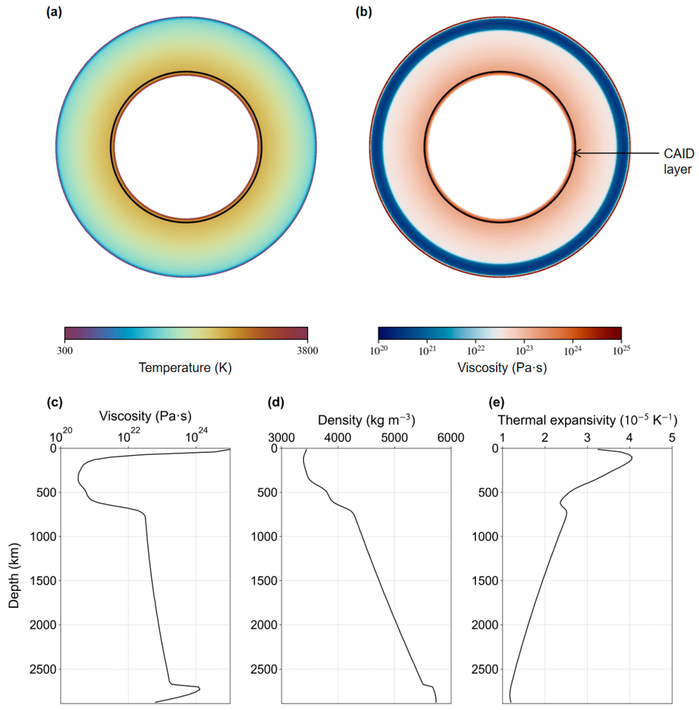
Figure 2 shows the initial conditions of our model. We prescribe velocities based on the supercontinent cycle on the model surface (details in the next section); the bottom is a free slip boundary. The fixed boundary temperatures are 3800 K at the bottom and 300 K at the top. The CAID layer initially covers the CMB with a height of 150 km [21]. Each case runs for 3000 Myr.

In the top 1000 km of the model, the minimum resolution of the mesh is about 25 km, while in other regions, the minimum resolution is about 50 km. The mesh is adaptively refined according to gradients in viscosity, temperature, and composition fields.

2.4. Implementation of Supercontinent Cycle Modes

A supercontinent cycle period $\mathsf{\Delta }{t}_{sc}$ consists of two parts: the assembly period $\mathsf{\Delta }{t}_a$ and the breakup period $\mathsf{\Delta }{t}_b$. The total duration of the cycle, $\mathsf{\Delta }{t}_{\mathrm{s}\mathrm{c}}$, is therefore given by Equation (12):

$$\mathsf{\Delta }{t}_{sc}=\mathsf{\Delta }{t}_a+\mathsf{\Delta }{t}_b$$

(12)

According to current geological records, the general supercontinent cycle has a period of ~600 Myr, including assembly and breakup periods, and the assembly duration ranges from 100 to 300 Myr [4]. Here we assume 1/3 of the cycle for the assembly, and the remaining 2/3 for the breakup.

The continental velocity $V_{con}$ is related to supercontinent breakup period $\mathsf{\Delta }{t}_b$, by Equation (13):

$$V_{con}={\displaystyle \frac{\mathrm{S}}{\mathsf{\Delta }{t}_b}}$$

(13)

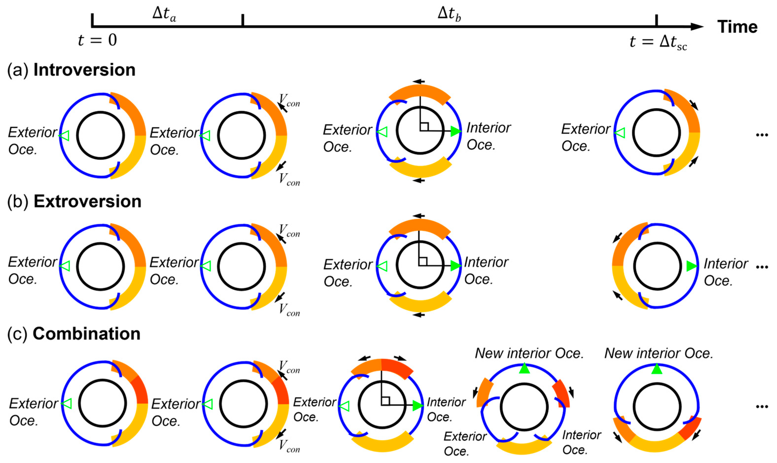
Here, S represents the distance of continental motion in a supercontinent cycle, which varies among the three supercontinent cycle modes as illustrated in Figure 3.

Oceanic plates are divided into interior and exterior oceans. The velocity of the exterior ocean, $V_{oce-ex}=6.6\mathrm{c}\mathrm{m}/\mathrm{y}\mathrm{r}$, follows Argus et al. [36] and the velocity of the interior ocean is assumed to equal the velocity of the continental plates, i.e., $V_{oce-in}=V_{con}$.

We implement three modes of the supercontinent cycle—introversion, extroversion, and combination—following the conceptual models of Yoshida [14,15]. The fundamental distinction among these three modes lies in which ocean closes: extroversion closes the exterior ocean, introversion closes the interior ocean, and the combination mode involves the closure of both oceans (Figure 3).

In the introversion mode (Figure 3a), the supercontinent motion could be divided into four stages. First, at $t=0$ and during the assembly period, the supercontinent remains stationary, while subduction occurs in the exterior ocean. Second, at $t=\mathsf{\Delta }{t}_a$, the supercontinent begins to break up, producing two equally sized new continents moving away from each other. Third, in the introversion mode, the two continents from supercontinent breakup migrate to positions approximately 90° from the former supercontinent. Finally, at $t=\mathsf{\Delta }{t}_a+\mathsf{\Delta }{t}_b$, the two continents assemble into a new supercontinent through the closure of the interior ocean.

In the extroversion mode (Figure 3b), the overall process is similar. The only difference is that, after the two continents from supercontinent breakup migrate to positions 90° away from the initial supercontinent, a new supercontinent assembles through the closure of the exterior ocean.

In the combination mode (Figure 3c), the process consists of five stages, with the first three stages being identical to those in the introversion and extroversion modes. During the fourth stage, which occurs in the breakup period, the two continents close neither the interior ocean nor the exterior ocean, in contrast to the introversion and extroversion modes. Instead, one continent remains stationary, whereas another undergoes further breakup into two smaller continents. These two smaller continents move away from each other, generating a new interior ocean. Finally, the three continents assemble into a new supercontinent through the combined closure of the interior and exterior oceans.

2.5. Experiment Design

The supercontinent cycle was driven by pre-defined boundary velocities with different periods (400, 600, and 800 Myr) and different modes (introversion, extroversion, combination). Eighteen experimental cases are designed, covering the parameter space of “supercontinent cycle mode (3 types) × cycle period (3 types) × with or without CAID layer” (

Table 3. Experimental setting.

Case ID	CAID Layer Presence?	Cycle Mode	Period (Myr)
N_I_400	No	Introversion	400
N_I_600	No	Introversion	600
N_I_800	No	Introversion	800
N_E_400	No	Extroversion	400
N_E_600	No	Extroversion	600
N_E_800	No	Extroversion	800
N_C_400	No	Combination	400
N_C_600	No	Combination	600
N_C_800	No	Combination	800
Y_I_400	Yes	Introversion	400
Y_I_600	Yes	Introversion	600
Y_I_800	Yes	Introversion	800
Y_E_400	Yes	Extroversion	400
Y_E_600	Yes	Extroversion	600
Y_E_800	Yes	Extroversion	800
Y_C_400	Yes	Combination	400
Y_C_600	Yes	Combination	600
Y_C_800	Yes	Combination	800

).

Because the $∆{\rho }_c$ of the CAID layer directly determines the reliability of the conclusions, and because considerable uncertainty exists in the reported $∆{\rho }_c$ in previous studies [37,38], a sensitivity test is conducted for this parameter. In addition to the reference density (150 kg m⁻³), three different densities (50, 100, and 200 kg m⁻³) are tested to assess the sensitivity of the results.

2.6. Calculation of Global Plume Heat Flux

The global plume heat flux is computed following the method of Li et al. [39], plume regions $S_{plume}$ were identified by the criteria that the radial velocity is positive and the temperature satisfies the condition in Equation (14):

$$T>T_{bg}+f$$

(14)

Here, $f$ is an excess temperature threshold, and $T_{bg}$ is the laterally averaged temperature excluding relatively cold (e.g., downwelling) regions where $T\le T_{ave}$, with $T_{ave}$ being the laterally averaged temperature. Following Li et al. [39], an excess temperature of 200 K was adopted, as they showed that changing this threshold alters the absolute magnitude of the heat flux but does not affect its temporal trend.

The global plume heat flux $Q_p$ at a given depth was then obtained by integrating the heat flux over all identified plume regions by Equation (15):

$$Q_p={\int }_{S_{plume}}\rho C_p{u}_r\left(T-T_{bg}\right)dS$$

(15)

where $\rho$ is the density, $C_p$ the specific heat capacity, $u_r$ the radial velocity, and $T_{bg}$ the laterally averaged background temperature.

In this study, the global plume heat flux is calculated at a depth of 700 km, following Li et al. [39], which provides a balance between adequate resolution in the lower mantle and reduced influence of complex upper-mantle rheology.

2.7. Analytical Method for Global Plume Heat Flux

To extract periodic signals from the global heat flux time series, we applied the Lomb–Scargle periodogram [40,41], which is well suited for unevenly sampled data and does not require interpolation. Before analysis, we removed the data corresponding to the first supercontinent cycle and detrended the remaining series.

We assessed statistical significance using a sieve bootstrap approach [42]. We first fit an autoregressive (AR) model to the series. We then generate 2000 surrogate time series by resampling the residuals of the AR model and reconstructing the signal using the estimated AR coefficients. The 95% and 99% background spectral power levels are used as significance thresholds. A spectral peak is considered statistically significant if its power exceeds the 95% confidence level.

Among the identified significant peaks, we take the period with the highest spectral peak as the dominant period of the global plume heat flux, and compare it with the supercontinent cycle period. If the absolute deviation between the two periods is ≤ 50 Myr, the period of global plume heat flux is considered in agreement with the cycle period; otherwise, it is considered not in agreement with the cycle period.

To quantitatively extract the phase of the periodic global plume heat flux signal, we first perform event-aligned averaging analysis. We define the time of supercontinent assembly completion as the event reference and use the duration of each supercontinent cycle as the time window. The event-aligned average curve was then fitted with a sine function of the form given by Equation (16):

$$f(t)=A\mathrm{s}\mathrm{i}\mathrm{n}({\displaystyle \frac{2\pi }{T}}t+\varphi )+C$$

(16)

Here, $A$ is the amplitude, $T$ the dominant period determined from the Lomb–Scargle power spectrum, $\varphi$ the phase offset, and $C$ a constant. The parameters are optimized via least squares. The goodness of fit is evaluated by the coefficient of determination R². The time offset $t_p$ is the time at which the fitted sine curve reaches its maximum.

$$f(t)=A_1\mathrm{s}\mathrm{i}\mathrm{n}\left({\displaystyle \frac{2\pi }{T_1}}t+{\varphi }_1\right)+A_2\mathrm{s}\mathrm{i}\mathrm{n}\left({\displaystyle \frac{2\pi }{T_2}}t+{\varphi }_2\right)+C$$

(17)

For the combination mode, the global plume heat flux curves, showing a pronounced dual-peak structure, are fitted using a double sine procedure given by Equation (17). The two dominant periods ($T_1$ and $T_2$) are identified from the Lomb–Scargle power spectra, and the time offset $t_p$ was calculated using the same method as discussed above.

3. Results

3.1. The Overall Trend of Thermal Evolution

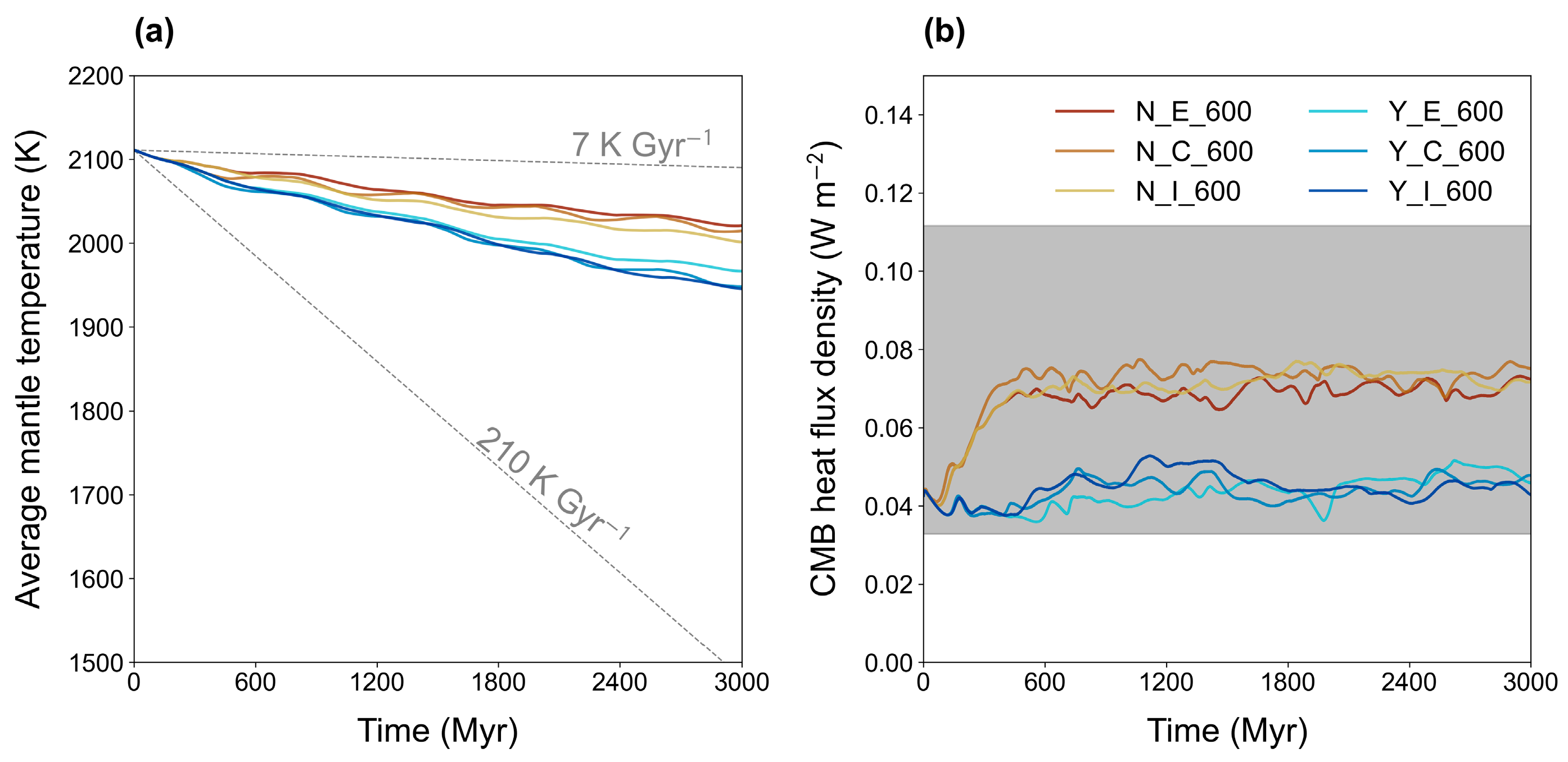
To verify if our models reproduce the thermal evolution of Earth’s mantle, we examine the average mantle temperature and CMB heat flux density. Figure 4 displays these quantities for six representative models with a 600 Myr supercontinent cycle. All cases exhibit a cooling trend, with the average mantle temperature decreasing by approximately 90–150 K over a 3000 Myr simulation period (Figure 4a). The corresponding cooling rates range from 30 to 50 K Gyr⁻¹, well within the inferred range of 7–210 K Gyr⁻¹ for Earth’s mantle [43]. Meanwhile, the CMB heat flux density in the cases stabilizes between 0.04 and 0.07 W m⁻² (Figure 4b), consistent with independent estimates of Earth’s present-day CMB heat flux density (0.03–0.11 W m⁻²) [43,44]. Neither the presence of a CAID layer nor the supercontinent cycle mode has a significant impact on the average mantle temperature, values in all cases remain within the reported ranges.

3.2. Global Plume Heat Flux Periodicity

To assess whether the presence of a CAID layer is necessary for periodic behavior in global plume heat flux, we compared cases with and without a CAID layer in three supercontinent cycle periods (400, 600, and 800 Myr). The effect of the CAID layer is similar across the introversion, extroversion, and combination modes. We present detailed results of the extroversion mode as a representative case, while a comprehensive summary of all 18 cases is provided in

Table A1. Dominant periods of global plume heat flux in all models.

Case ID	Cycle Mode	Period (Myr)	CAID Layer Presence?	Dominant Period (Myr)	Significance (%)	Matched?
Y_I_400	Introversion	400	Yes	411	99	Yes
N_I_400	Introversion	400	No	400	100	Yes
Y_I_600	Introversion	600	Yes	603	97	Yes
N_I_600	Introversion	600	No	69	99	No
Y_I_800	Introversion	800	Yes	255	98	No
N_I_800	Introversion	800	No	70	98	No
Y_E_400	Extroversion	400	Yes	393	100	Yes
N_E_400	Extroversion	400	No	408	99	Yes
Y_E_600	Extroversion	600	Yes	643	100	Yes
N_E_600	Extroversion	600	No	47	100	No
Y_E_800	Extroversion	800	Yes	122	100	No
N_E_800	Extroversion	800	No	81	98	No
Y_C_400	Combination	400	Yes	401	99	Yes
N_C_400	Combination	400	No	431	95	Yes
Y_C_600	Combination	600	Yes	587	97	Yes
N_C_600	Combination	600	No	144	96	No
Y_C_800	Combination	800	Yes	814	95	Yes
N_C_800	Combination	800	No	39	100	No

in the Appendix A.

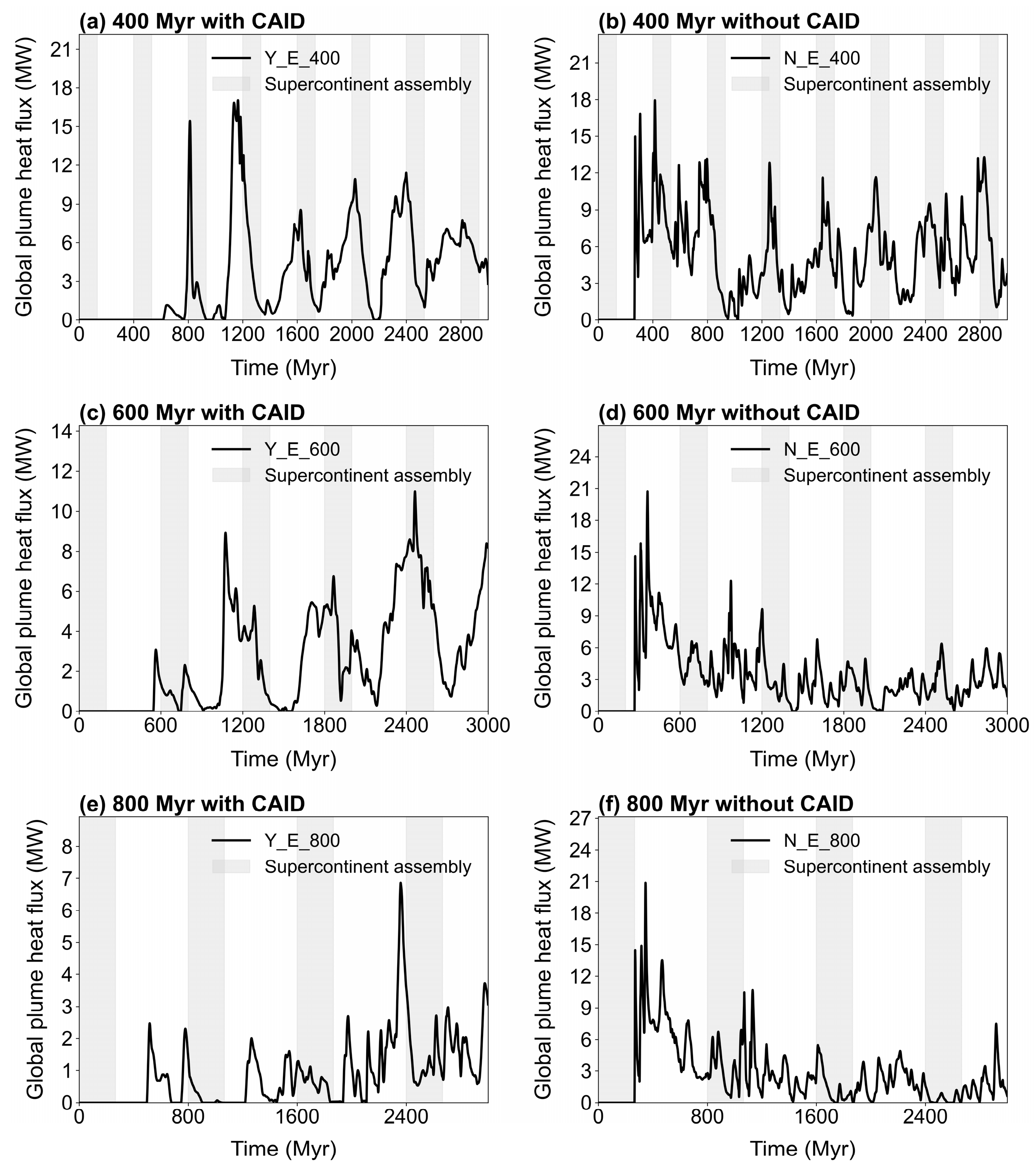
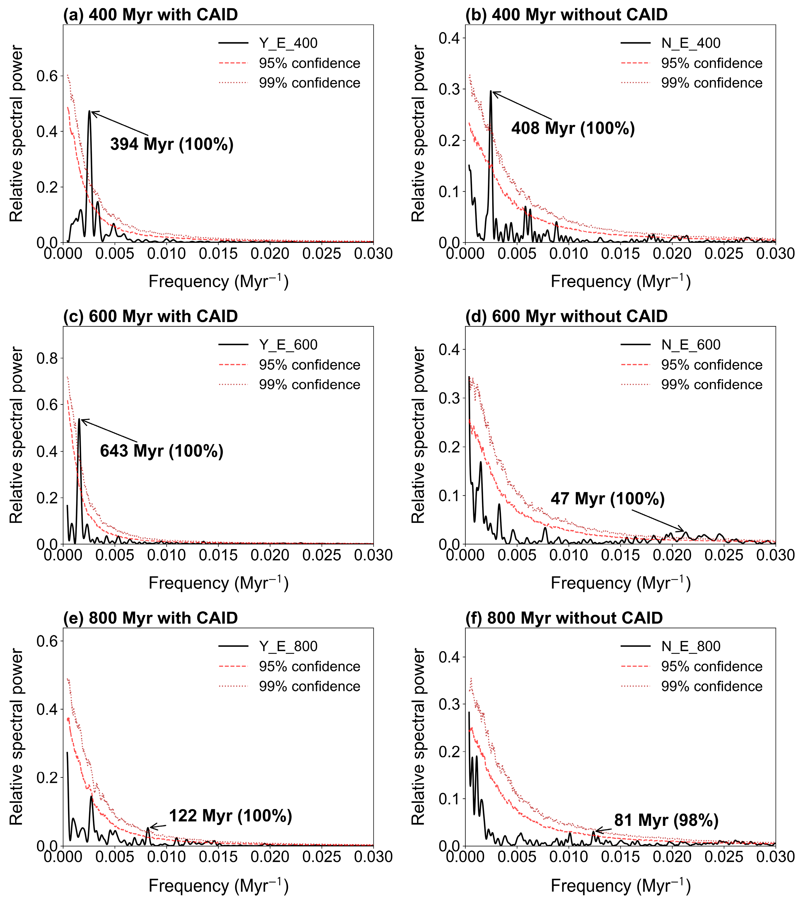
For the 400 Myr cycle (Figure 5a,b and Figure 6a,b), both cases with a CAID layer (Y_E_400) and those without a CAID layer (N_E_400) exhibit clear periodic fluctuations, with a period equal to the supercontinent cycle period. The dominant periods are 393 Myr and 408 Myr, respectively, both exceeding the 99% significance level. At this short supercontinent cycle period, when continental motions are rapid, a CAID layer is not required for global plume heat flux to display periodic behavior.

For the 600 Myr cycle, the contrast between cases with and without a CAID layer is striking (Figure 5c,d and Figure 6c,d). The case with a CAID layer (Y_E_600) exhibits evident periodic fluctuations with a period of 643 Myr, matching the supercontinent cycle period and exceeding the 99% significance level. In contrast, the case without a CAID layer (N_E_600) exhibits a dominant period of 47 Myr, not matching the 600 Myr supercontinent cycle period. At this intermediate supercontinent cycle period, the presence of a CAID layer is necessary for global plume heat flux to display periodic behavior.

For the 800 Myr cycle (Figure 5e,f and Figure 6e,f), neither case exhibits periodic fluctuations that can match the supercontinent cycle period. The case with a CAID layer (Y_E_800) exhibits a dominant period of 122 Myr, exceeding the 99% significance threshold, while the case without a CAID layer (N_E_800) shows a dominant period of 81 Myr, also exceeding the 95% significance threshold.

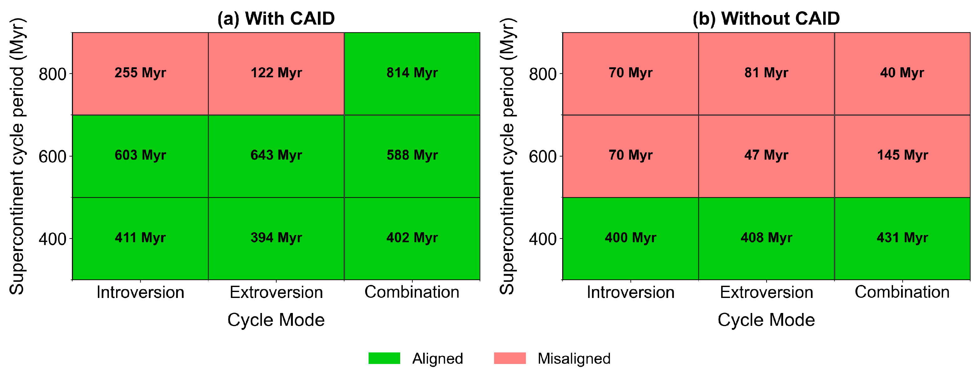
All 18 cases (Figure 7) show that the presence of a CAID layer plays a significant role in the periodicity of global plume heat flux. During rapid continental motion (400 Myr cycle), the external forcing is likely sufficient to drive global plume heat flux to a period equal to that of the supercontinent cycle, regardless of the presence of a CAID layer. During intermediate continental motion (600 Myr cycle), the presence of a CAID layer is necessary for global plume heat flux period to match the supercontinent cycle period. During slow continental motion (800 Myr cycle), even with a CAID layer, the periodicity of global plume heat flux does not align with the supercontinent cycle periodicity. However, an exception is observed in case Y_C_800, in which the dominant period matches the supercontinent cycle period.

3.3. Time Offset of Global Plume Heat Flux

Having established the conditions under which global plume heat flux periodicity aligns with the supercontinent cycle periodicity, we further examine, particularly in the ten aligned cases (Figure 7), how the cycle mode influences the time offset relative to supercontinent assembly.

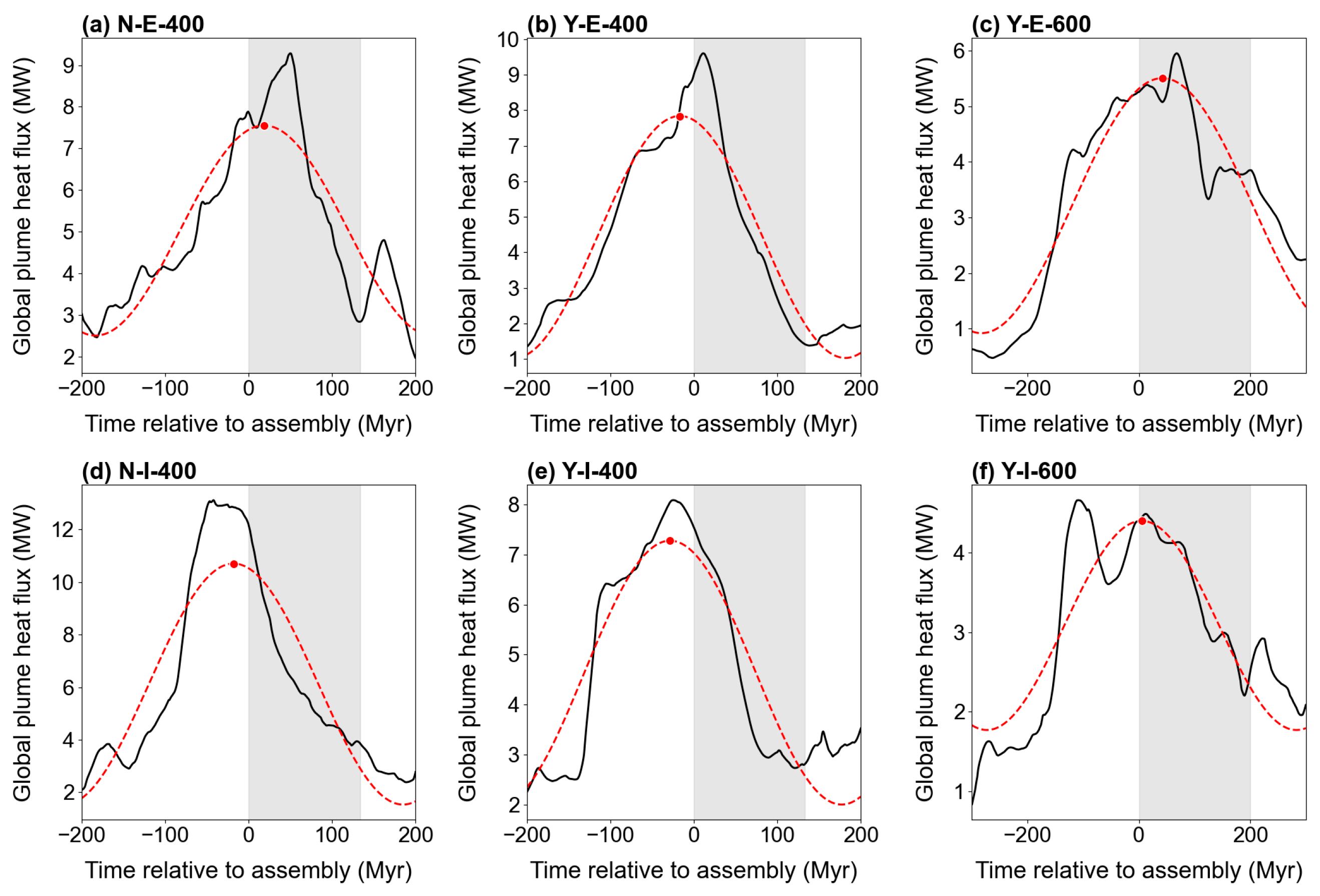
Figure 8 presents the global plume heat flux curves along with their sine fits for both the introversion and extroversion modes with the 400 and 600 Myr periods. The sine fits show good agreement with the data (

Table 4. Phase analysis results.

Case ID	Cycle Mode	Period (Myr)	${\mathit{t}}_{\mathit{p}}$ (Myr)	R2
N_I_400	Introversion	400	−17	0.82
N_E_400	Extroversion	400	18	0.82
N_C_400	Combination	400	−162	0.86
Y_I_400	Introversion	400	−28	0.84
Y_I_600	Introversion	600	5	0.79
Y_E_400	Extroversion	400	−16	0.91
Y_E_600	Extroversion	600	42	0.89
Y_C_400	Combination	400	−163	0.70
Y_C_600	Combination	600	−234	0.89
Y_C_800	Combination	800	−364	0.80

). Overall, the fitted sine curve reaches its maximum for both the introversion and extroversion modes near the time of supercontinent assembly completion. Within each period, the corresponding time offsets for the introversion mode are smaller than those for the extroversion mode. Specifically, when the CAID layer is present, for the 400 Myr period, time offset is −28 Myr for the introversion mode and −16 Myr for the extroversion mode, while for the 600 Myr period, the time offset is 5 Myr for the introversion mode and 42 Myr for the extroversion mode. When the CAID layer is absent, for the 400 Myr period, the time offset is −17 Myr for the introversion mode and 18 Myr for the extroversion mode.

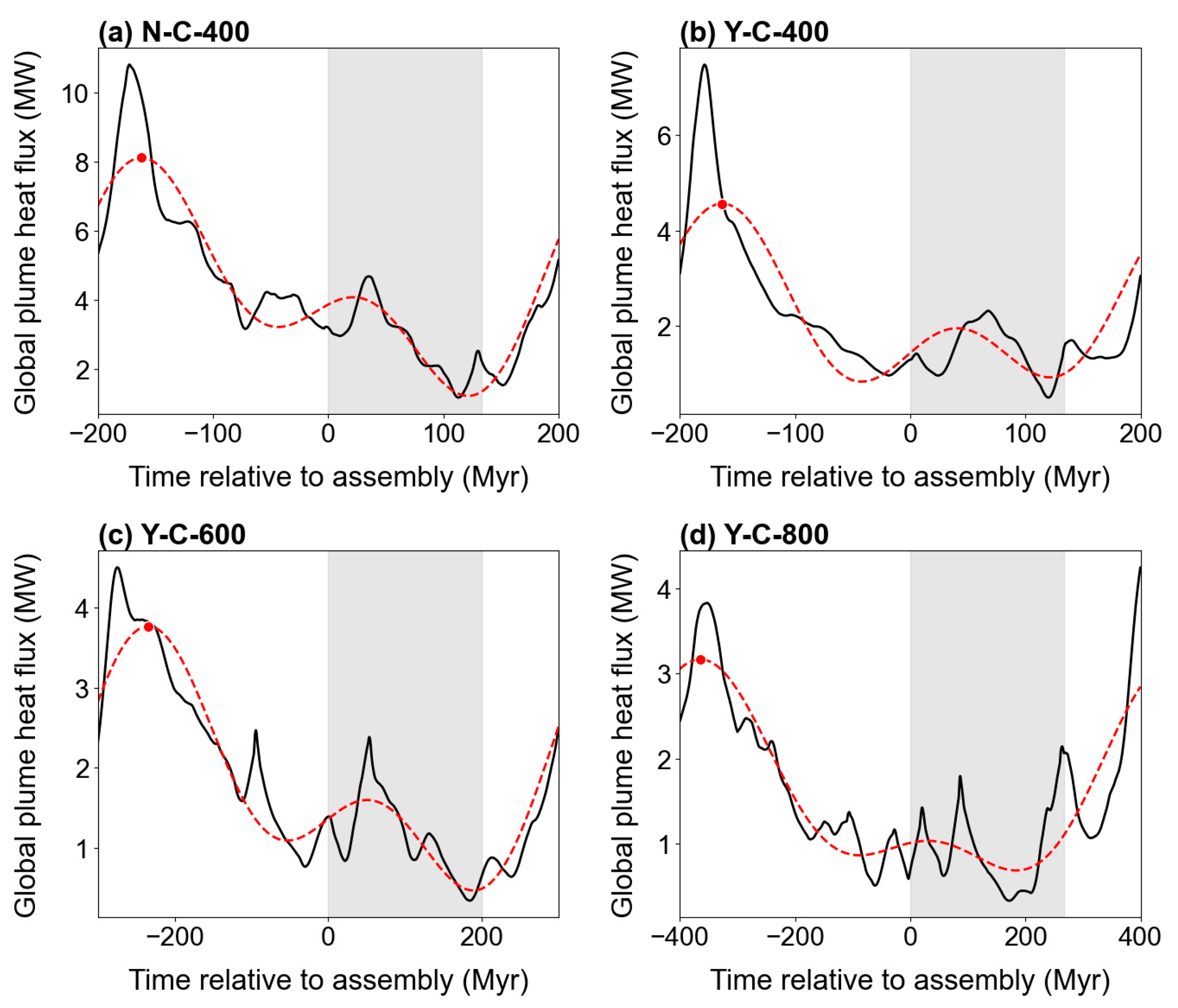
The global plume heat flux in the combination mode exhibits a more complex pattern, characterized by a dual-peak structure (Figure 9). Double sine fits show good agreement with the data (Table 4). The corresponding time offsets are −162, −163, −234, and −364 Myr, indicating that the peaks of the global plume heat flux occur far from the time of supercontinent assembly completion.

3.4. Sensitivity Analysis

In the preceding analyses, the $∆{\rho }_c$ of CAID was assigned a reference value of 150 kg m⁻³. In the corresponding sensitivity test, the $∆{\rho }_c$ was varied from 50 to 200 kg m⁻³ with reference to Guerrero et al. [45] and Yang and Fu [46], results are shown in

Table 5. Results of the sensitivity analysis.

Cycle Mode	$∆{\mathit{\rho }}_{\mathit{c}}$ (kg m−3)	Dominant Period (Myr)	Matched?	${\mathit{t}}_{\mathit{p}}$ (Myr)
Introversion	50	479	No	−44
Introversion	100	632	Yes	3
Introversion	150	603	Yes	5
Introversion	200	591	Yes	17
Extroversion	50	270	No	4
Extroversion	100	632	Yes	12
Extroversion	150	643	Yes	42
Extroversion	200	627	Yes	33
Combination	50	272	No	98
Combination	100	632	Yes	−235
Combination	150	587	Yes	−234
Combination	200	602	Yes	−276

. For all results, the global plume heat flux period does not match the supercontinent cycle period only when the CAID density difference is 50 kg m⁻³, while the global plume heat flux period matches the supercontinent cycle period under all other conditions. Meanwhile, for the same cycle period, time offset for the introversion mode is smaller than that for the extroversion mode. These results indicate that the preceding findings are robust, except under the low-density condition (50 kg m⁻³), and the CAID density differences between 100 and 200 kg m⁻³ do not affect the robustness of the conclusions.

4. Discussion

LIP events are recorded throughout Earth’s geological history, and represent the surface manifestation of the association between mantle and plate tectonics [47]. Observational and theoretical studies have provided evidence, including hotspot volcanism records mantle-plume activity [48], plume heads trigger the formation of LIPs [47], and LIPs preferentially occur at the margins of LLSVPs [49]. Together, these lines of evidence suggest that LIP events, as surface manifestations, can serve as observable indicators of variations in mantle and plume heat flux.

Geological records suggest that LIP cycles exhibit a periodicity of approximately 750–550 Myr [28]. In addition, there is a phase lag between supercontinent assembly and LIP activity. For each supercontinent, the first major episode of plume breakout, marked by the first LIP event, occurs only after the completion of supercontinent assembly [4]. The first LIP record of Pangaea lags supercontinent assembly by approximately 75 Myr, whereas the lag time for Rodinia ranges from about 20 to 120 Myr [29]. In our experiments, we use the calculated global plume heat flux at a depth of 700 km as an indirect proxy for LIP activity. Based on our analysis, we interpret the time of peak global plume heat flux during each supercontinent cycle as an approximate estimate of the time of the first LIP event.

Our results show that supercontinent cycles influence both the periodicity and phase of global plume heat flux. We find that the cycle period is the primary factor controlling the periodicity of global plume heat flux, and this periodicity is also affected by the presence or absence of the CAID layer. For cases under rapid continental motion (400 Myr cycle period), the global plume heat flux period always matches the supercontinent cycle period. Conversely, under slow continental motion (800 Myr cycle period), the global plume heat flux period rarely aligns with the cycle period. For the 600 Myr cycle period, CAID material helps establish a mechanism by which the supercontinent cycle drives globally periodic subduction and, consequently, periodic mantle plume generation. The role of CAID material in promoting this process may be comparable to the mechanisms proposed in previous studies. Heyn et al. [50] indicated that localized subduction can induce periodic plume generation from the dense material. Furthermore, Kameyama and Harada [51] have suggested that the dense material moves laterally in response to the motion of the overlying supercontinent, which in turn deflects upwelling plume conduits horizontally and facilitates the breakup of the newly assembled supercontinent.

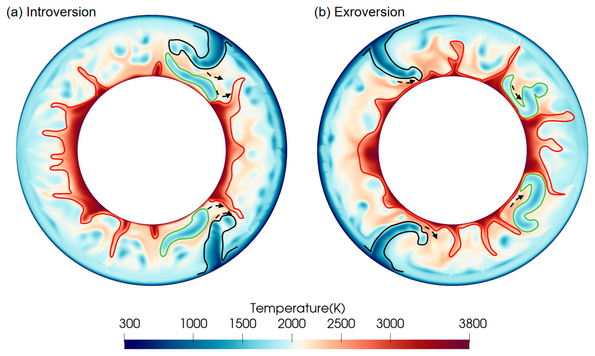
We find that the supercontinent cycle mode significantly affects the phase of global plume heat flux. For both the introversion and extroversion modes, each cycle has a single peak in global plume heat flux near the completion of supercontinent assembly. The time of the peak in global heat flux relative to assembly completion is earlier in the introversion mode than in the extroversion mode. These differences in global plume heat flux peak timing among supercontinent cycle modes can be attributed to variations in subduction locations during the cycle, which alter the distribution of plumes [52]. The locations of subduction differ among our models, with introversion closing the interior ocean and extroversion closing the exterior ocean. Subduction not only affects plume distribution but also influences plume intensity. In our model, the subducting plate descends adjacent to the evolving plume (Figure 10, black line), a configuration that has been shown to promote plume development, as described in detail by Plimmer et al. [53] In the introversion mode, the current slabs descend near the slabs inherited from the latest supercontinent cycle, reinforcing plume upwelling and thereby promoting plume development. In the extroversion mode, however, the current slabs and the inherited slabs are antipodal, which weakens the influence of subduction on plume development relative to the introversion mode (see Videos S1 and S2). In the combination mode, locations of subduction differ markedly from both the introversion and extroversion modes (Video S3), and its phase of global plume heat flux shift relative to assembly completion also differs from the other two modes.

In contrast, in the combination mode, the global plume heat flux exhibits a dual-peak structure in which the larger peaks from the double sine fitting occur significantly earlier relative to the completion of supercontinent assembly (at −162, −163, −234, and −364 Myr, respectively, during the breakup period; Figure 9). During the breakup period in the combination mode, plates reorganize (Figure 3c), accompanied by the closure of both internal and external oceans and large-scale subduction (Video S3), thereby leading to peaks of global plume heat flux. However, the smaller peaks from the double sine fitting in the assembly period appear later than the assembly (at 22, 41, 51, and 30 Myr, respectively; Figure 9). In the combination mode of this study, the global plume heat flux displays larger peaks during the breakup period; perhaps the smaller peaks during the assembly period more genuinely reflect the mantle’s response to the supercontinent cycle. Advances in palaeo geographic reconstructions and three-dimensional geodynamic modelling are providing a clearer picture of the supercontinent cycle [54,55,56,57] wherein, in a true three-dimensional Earth and for a combination mode involving multiple continental blocks, the motion paths of continents during assembly and breakup follow certain regularities, such as true polar wander (TPW) [58,59]. The mantle heat flux under the influence of the supercontinent cycle in the combination mode will be revealed more accurately in three-dimensional simulations; nevertheless, incorporating supercontinent motion paths that account for mantle–plate interactions remains a considerable challenge for numerical modelling at present.

Our study compares the time of simulated global plume heat flux peaks with the occurrence of the first LIP events, as LIP events are influenced by factors such as plume ascent velocity and the latent heat of phase transitions [60,61], the time of LIP events is expected to lag behind that of the plume heat flux. Accounting for the expected delay of actual LIP events, particularly at the currently favored 600 Myr supercontinent cycle [4], we propose that, both in the introversion and extroversion modes, the time of the peak in global heat flux coincides with the time of the first LIP event (5 Myr for Y_I_600 and 42 Myr for Y_E_600 in Table 4), and lags behind the time of supercontinent assembly completion (20–120 Myr for Rodinia, 75 Myr for Pangaea). These results thus support the idea that supercontinent assembly modifies mantle dynamics, and that mantle plumes, in turn, influence the breakup of the supercontinent [29].

Using two-dimensional models, this study reveals robust periodicity in plume activity. In two-dimensional geometry, mantle upwellings take the form of sheet-like structures rather than point-source cylindrical plumes, which affects the absolute magnitude of plume heat flux but is unlikely to alter the periodicity of the global plume heat flux. This is because periodicity is controlled by the boundary conditions rather than by individual plume geometry. The plume heat flux periodicity in our two-dimensional model aligns with the three-dimensional results of Li et al. [39], yet their calculated period remains smaller than ours as it does not account for the supercontinent cycle. Nonetheless, the quantitative phase offsets (e.g., −28 Myr vs. +42 Myr for introversion vs. extroversion) are model-dependent and may be quantitatively unreliable in two dimensions; therefore, these should be verified by three-dimensional models, as three-dimensional geometry allows for more complex subduction belt configurations.

5. Conclusions

Our numerical experiments show that the supercontinent cycle controls mantle plume activity, with the cycle period regulating the periodicity of global plume heat flux. In addition, the CAID layer is essential for the period of global plume heat flux to match the 600 Myr supercontinent cycle. Beyond periodicity, the cycle mode controls the time of peak global plume heat flux, introversion accelerates plume upwelling and causes the global plume heat flux to peak earlier; extroversion leads to a later peak; and the combination mode produces a dual-peak structure. For the introversion and extroversion modes, the simulated peak in global plume heat flux occurs shortly after the completion of supercontinent assembly, broadly consistent with the timing of the first LIP event in the geological record. These results provide new insights into how deep mantle dynamics respond to, and feed back on, surface tectonic reorganization. Still, as our results stem from two-dimensional models with kinematically prescribed plates, three-dimensional models incorporating self-consistent dynamics are required to validate and refine these temporal relationships.

References

1. Murphy, J.B.; Nance, R.D. Speculations on the Mechanisms for the Formation and Breakup of Supercontinents. Geosci. Front. 2013, 4, 185–194. [Google Scholar] [CrossRef]
2. Evans, D.A.D.; Li, Z.X.; Murphy, J.B. Four-Dimensional Context of Earth’s Supercontinents. Geol. Soc. Lond. Spec. Publ. 2016, 424, 1–14. [Google Scholar] [CrossRef]
3. Meert, J.G. What’s in a Name? The Columbia (Paleopangaea/Nuna) Supercontinent. Gondwana Res. 2012, 21, 987–993. [Google Scholar] [CrossRef]
4. Mitchell, R.N.; Zhang, N.; Salminen, J.; Liu, Y.; Spencer, C.J.; Steinberger, B.; Murphy, J.B.; Li, Z.-X. The Supercontinent Cycle. Nat. Rev. Earth Environ. 2021, 2, 358–374. [Google Scholar] [CrossRef]
5. Li, Z.X.; Mitchell, R.N.; Spencer, C.J.; Ernst, R.; Pisarevsky, S.; Kirscher, U.; Murphy, J.B. Decoding Earth’s Rhythms: Modulation of Supercontinent Cycles by Longer Superocean Episodes. Precambrian Res. 2019, 323, 1–5. [Google Scholar] [CrossRef]
6. Murphy, J.; Nance, R.; Cawood, P. Contrasting Modes of Supercontinent Formation and the Conundrum of Pangea. Gondwana Res. 2009, 15, 408–420. [Google Scholar] [CrossRef]
7. Hartnady, C.J.H. About Turn for Supercontinents. Nature 1991, 352, 476–478. [Google Scholar] [CrossRef]
8. Nance, R.D.; Worsley, T.R.; Moody, J.B. The Supercontinent Cycle. Sci. Am. 1988, 259, 72–79. [Google Scholar] [CrossRef]
9. Nance, R.D.; Murphy, J.B.; Santosh, M. The Supercontinent Cycle: A Retrospective Essay. Gondwana Res. 2014, 25, 4–29. [Google Scholar] [CrossRef]
10. Donnadieu, Y.; Goddéris, Y.; Ramstein, G.; Nédélec, A.; Meert, J. A ‘Snowball Earth’ Climate Triggered by Continental Break-up through Changes in Runoff. Nature 2004, 428, 303–306. [Google Scholar] [CrossRef] [PubMed]
11. Campbell, I.H.; Allen, C.M. Formation of Supercontinents Linked to Increases in Atmospheric Oxygen. Nat. Geosci. 2008, 1, 554–558. [Google Scholar] [CrossRef]
12. Hoffman, P.F.; Kaufman, A.J.; Halverson, G.P.; Schrag, D.P. A Neoproterozoic Snowball Earth. Science 1998, 281, 1342–1346. [Google Scholar] [CrossRef]
13. Wignall, P.B. Large Igneous Provinces and Mass Extinctions. Earth-Sci. Rev. 2001, 53, 1–33. [Google Scholar] [CrossRef]
14. Yoshida, M. Effect of the Supercontinent Cycle on the Longest-Term Sea-Level Change from a Simple Conceptual and Theoretical Model. Gondwana Res. 2024, 125, 425–445. [Google Scholar] [CrossRef]
15. Yoshida, M. Long-Term Fluctuation of Earth’s Surface Heat Flux by the Supercontinent Cycle. Gondwana Res. 2025, 140, 146–157. [Google Scholar] [CrossRef]
16. Yoshida, M.; Santosh, M. Mantle Convection Modeling of the Supercontinent Cycle: Introversion, Extroversion, or a Combination? Geosci. Front. 2014, 5, 77–81. [Google Scholar] [CrossRef]
17. Mitchell, R.N.; Kilian, T.M.; Evans, D.A.D. Supercontinent Cycles and the Calculation of Absolute Palaeolongitude in Deep Time. Nature 2012, 482, 208–211. [Google Scholar] [CrossRef]
18. Dannberg, J.; Gassmöller, R.; Thallner, D.; LaCombe, F.; Sprain, C. Changes in Core–Mantle Boundary Heat Flux Patterns throughout the Supercontinent Cycle. Geophys. J. Int. 2024, 237, 1251–1274. [Google Scholar] [CrossRef]
19. Doucet, L.S.; Li, Z.-X.; Ernst, R.E.; Kirscher, U.; El Dien, H.G.; Mitchell, R.N. Coupled Supercontinent–Mantle Plume Events Evidenced by Oceanic Plume Record. Geology 2019, 48, 159–163. [Google Scholar] [CrossRef]
20. Heron, P.J.; Dannberg, J.; Gassmöller, R.; Shephard, G.E.; van Hunen, J.; Pysklywec, R.N. The Impact of Pangean Subducted Oceans on Mantle Dynamics: Passive Piles and the Positioning of Deep Mantle Plumes. Gondwana Res. 2025, 138, 168–185. [Google Scholar] [CrossRef]
21. Trim, S.J.; Lowman, J.P. Interaction between the Supercontinent Cycle and the Evolution of Intrinsically Dense Provinces in the Deep Mantle. J. Geophys. Res. Solid Earth 2016, 121, 8941–8969. [Google Scholar] [CrossRef]
22. Gleeson, M.; Soderman, C.; Matthews, S.; Cottaar, S.; Gibson, S. Geochemical Constraints on the Structure of the Earth’s Deep Mantle and the Origin of the LLSVPs. Geochem. Geophys. Geosyst. 2021, 22, e2021GC009932. [Google Scholar] [CrossRef]
23. Puchkov, V.N. Relationship Between Plume and Plate Tectonics. Geotectonics 2016, 50, 425–438. [Google Scholar] [CrossRef]
24. Davies, D.R.; Goes, S.; Davies, J.H.; Schuberth, B.S.A.; Bunge, H.-P.; Ritsema, J. Reconciling Dynamic and Seismic Models of Earth’s Lower Mantle: The Dominant Role of Thermal Heterogeneity. Earth Planet. Sci. Lett. 2012, 353–354, 253–269. [Google Scholar] [CrossRef]
25. Davies, D.R.; Goes, S.; Lau, H.C.P. Thermally Dominated Deep Mantle LLSVPs: A Review. In The Earth’s Heterogeneous Mantle: A Geophysical, Geodynamical, and Geochemical Perspective; Khan, A., Deschamps, F., Eds.; Springer International Publishing: Cham, Switzerland, 2015; pp. 441–477. [Google Scholar]
26. Liu, X.; Tian, F.; Li, J.; Li, Y.; Sun, W. The Evolution of Dense ULVZs Originating Outside LLSVPs and Implications for Dynamics at LLSVP Margins. J. Geophys. Res. Solid Earth 2024, 129, e2024JB028972. [Google Scholar] [CrossRef]
27. Langemeyer, S.M.; Lowman, J.P.; Tackley, P.J. The Dynamics and Impact of Compositionally Originating Provinces in a Mantle Convection Model Featuring Rheologically Obtained Plates. Geophys. J. Int. 2020, 220, 1700–1716. [Google Scholar] [CrossRef]
28. Prokoph, A.; Ernst, R.E.; Buchan, K.L. Time-Series Analysis of Large Igneous Provinces: 3500 Ma to Present. J. Geol. 2004, 112, 1–22. [Google Scholar] [CrossRef]
29. Li, Z.; Zhong, S. Supercontinent–Superplume Coupling, True Polar Wander and Plume Mobility: Plate Dominance in Whole-Mantle Tectonics. Phys. Earth Planet. Inter. 2009, 176, 143–156. [Google Scholar] [CrossRef]
30. Gassmöller, R.; Dannberg, J.; Bangerth, W.; Heister, T.; Myhill, R. On Formulations of Compressible Mantle Convection. Geophys. J. Int. 2020, 221, 1264–1280. [Google Scholar] [CrossRef]
31. Dannberg, J.; Heister, T. Compressible Magma/Mantle Dynamics: 3-D, Adaptive Simulations in ASPECT. Geophys. J. Int. 2016, 207, 1343–1366. [Google Scholar] [CrossRef]
32. Li, Y.; Deschamps, F.; Tackley, P.J. The Stability and Structure of Primordial Reservoirs in the Lower Mantle: Insights from Models of Thermochemical Convection in Three-Dimensional Spherical Geometry. Geophys. J. Int. 2014, 199, 914–930. [Google Scholar] [CrossRef]
33. Ulvrova, M.M.; Brune, S.; Williams, S. Breakup without Borders: How Continents Speed up and Slow down during Rifting. Geophys. Res. Lett. 2019, 46, 1338–1347. [Google Scholar] [CrossRef]
34. Tosi, N.; Yuen, D.A.; de Koker, N.; Wentzcovitch, R.M. Mantle Dynamics with Pressure- and Temperature-Dependent Thermal Expansivity and Conductivity. Phys. Earth Planet. Inter. 2013, 217, 48–58. [Google Scholar] [CrossRef]
35. Van Der Wiel, E.; Van Hinsbergen, D.J.J.; Thieulot, C.; Spakman, W. Linking Rates of Slab Sinking to Long-Term Lower Mantle Flow and Mixing. Earth Planet. Sci. Lett. 2024, 625, 118471. [Google Scholar] [CrossRef]
36. Argus, D.F.; Gordon, R.G.; DeMets, C. Geologically Current Motion of 56 Plates Relative to the No-Net-Rotation Reference Frame: NNR-MORVEL56. Geochem. Geophys. Geosyst. 2011, 12, Q11001. [Google Scholar] [CrossRef]
37. Koelemeijer, P.; Deuss, A.; Ritsema, J. Density Structure of Earth’s Lowermost Mantle from Stoneley Mode Splitting Observations. Nat. Commun. 2017, 8, 15241. [Google Scholar] [CrossRef]
38. Lau, H.C.P.; Mitrovica, J.X.; Davis, J.L.; Tromp, J.; Yang, H.-Y.; Al-Attar, D. Tidal Tomography Constrains Earth’s Deep-Mantle Buoyancy. Nature 2017, 551, 321–326. [Google Scholar] [CrossRef]
39. Li, M.; Puetz, S.; Condie, K.; Olson, P. Mantle Plume Heat Flux and Surface Motion Periodicities and Their Implications for the Growth of Continental Crust. Earth Planet. Sci. Lett. 2023, 611, 118148. [Google Scholar] [CrossRef]
40. Lomb, N.R. Least-Squares Frequency Analysis of Unequally Spaced Data. Astrophys. Space Sci. 1976, 39, 447–462. [Google Scholar] [CrossRef]
41. Scargle, J.D. Studies in Astronomical Time Series Analysis. II—Statistical Aspects of Spectral Analysis of Unevenly Spaced Data. Astrophys. J. 1982, 263, 835–853. [Google Scholar] [CrossRef]
42. Kreiss, J.-P.; Lahiri, S.N. Bootstrap Methods for Time Series. In Handbook of Statistics; Elsevier: Amsterdam, The Netherlands, 2012; Volume 30, pp. 3–26. [Google Scholar]
43. Jaupart, C.; Labrosse, S.; Lucazeau, F.; Mareschal, J.-C. Temperatures, Heat, and Energy in the Mantle of the Earth. In Treatise on Geophysics; Elsevier: Amsterdam, The Netherlands, 2015; pp. 223–270. [Google Scholar]
44. Nimmo, F. Energetics of the Core. In Treatise on Geophysics; Elsevier: Amsterdam, The Netherlands, 2007; pp. 31–65. [Google Scholar]
45. Guerrero, J.M.; Deschamps, F.; Hsieh, W.-P.; Tackley, P.J. The Combined Effect of Heterogeneous Thermal Conductivity, Chemical Density Contrast, and Heat-Producing Element Enrichment on the Stability of Primordial Reservoirs above the Core-Mantle Boundary. Earth Planet. Sci. Lett. 2024, 637, 118699. [Google Scholar] [CrossRef]
46. Yang, T.; Fu, R. Thermochemical Piles in the Lowermost Mantle and Their Evolution. Phys. Earth Planet. Inter. 2014, 236, 109–116. [Google Scholar] [CrossRef]
47. Hill, R.I.; Campbell, I.H.; Davies, G.F.; Griffiths, R.W. Mantle Plumes and Continental Tectonics. Science 1992, 256, 186–193. [Google Scholar] [CrossRef]
48. Morgan, W.J. Convection Plumes in the Lower Mantle. Nature 1971, 230, 42–43. [Google Scholar] [CrossRef]
49. Burke, K.; Steinberger, B.; Torsvik, T.H.; Smethurst, M.A. Plume Generation Zones at the Margins of Large Low Shear Velocity Provinces on the Core–Mantle Boundary. Earth Planet. Sci. Lett. 2008, 265, 49–60. [Google Scholar] [CrossRef]
50. Heyn, B.H.; Conrad, C.P.; Trønnes, R.G. How Thermochemical Piles Can (Periodically) Generate Plumes at Their Edges. J. Geophys. Res. Solid Earth 2020, 125, e2019JB018726. [Google Scholar] [CrossRef]
51. Kameyama, M.; Harada, A. Supercontinent Cycle and Thermochemical Structure in the Mantle: Inference from Two-Dimensional Numerical Simulations of Mantle Convection. Geosciences 2017, 7, 126. [Google Scholar] [CrossRef]
52. Cao, X.; Flament, N.; Bodur, Ö.; Müller, R. The Evolution of Basal Mantle Structure in Response to Supercontinent Aggregation and Dispersal. Sci. Rep. 2021, 11, 22967. [Google Scholar] [CrossRef]
53. Plimmer, A.; Davies, J.; Panton, J. Investigating the Effect of Lithosphere Thickness and Viscosity on Mantle Dynamics throughout the Supercontinent Cycle. Geochem. Geophys. Geosyst. 2024, 25, e2024GC011688. [Google Scholar] [CrossRef]
54. Li, Z.-X.; Liu, Y.; Ernst, R. A Dynamic 2000—540 Ma Earth History: From Cratonic Amalgamation to the Age of Supercontinent Cycle. Earth-Sci. Rev. 2023, 238, 104336. [Google Scholar] [CrossRef]
55. Evans, D.A.D. Reconstructing Pre-Pangean Supercontinents. Geol. Soc. Am. Bull. 2013, 125, 1735–1751. [Google Scholar] [CrossRef]
56. Cao, X.; Collins, A.S.; Pisarevsky, S.; Flament, N.; Li, S.; Hasterok, D.; Müller, R.D. Earth’s Tectonic and Plate Boundary Evolution over 1.8 Billion Years. Geosci. Front. 2024, 15, 101922. [Google Scholar] [CrossRef]
57. Merdith, A.S.; Williams, S.E.; Collins, A.S.; Tetley, M.G.; Mulder, J.A.; Blades, M.L.; Young, A.; Armistead, S.E.; Cannon, J.; Zahirovic, S.; et al. Extending Full-Plate Tectonic Models into Deep Time: Linking the Neoproterozoic and the Phanerozoic. Earth-Sci. Rev. 2021, 214, 103477. [Google Scholar] [CrossRef]
58. Wang, C.; Mitchell, R.N. True Polar Wander in the Earth System. Sci. China Earth Sci. 2023, 66, 1165–1184. [Google Scholar] [CrossRef]
59. Zhong, S.; Zhang, N.; Li, Z.-X.; Roberts, J.H. Supercontinent Cycles, True Polar Wander, and Very Long-Wavelength Mantle Convection. Earth Planet. Sci. Lett. 2007, 261, 551–564. [Google Scholar] [CrossRef]
60. d’Acremont, E.; Leroy, S.; Burov, E.B. Numerical Modelling of a Mantle Plume: The Plume Head–Lithosphere Interaction in the Formation of an Oceanic Large Igneous Province. Earth Planet. Sci. Lett. 2003, 206, 379–396. [Google Scholar] [CrossRef]
61. Bossmann, A.B.; Van Keken, P.E. Dynamics of Plumes in a Compressible Mantle with Phase Changes: Implications for Phase Boundary Topography. Phys. Earth Planet. Inter. 2013, 224, 21–31. [Google Scholar] [CrossRef]
Figure 2. Initial conditions of the models. (a) Initial temperature field. (b) Initial viscosity field. The black line indicated by the arrow shows the contour of the initial CAID layer. (ce) Initial depth variations of viscosity, density, and thermal expansivity, respectively.
Applsci 16 05888 g002
Figure 3. Schematic of the supercontinent cycle, showing (a) introversion, (b) extroversion, and (c) combination modes. From left to right, one complete supercontinent cycle ( Δ t s c ) is shown, with Δ t a is assembly period, and Δ t b is breakup period. The thick orange and thin blue arcs indicate the continental and oceanic plates, respectively. Open and solid green triangles indicate the positions of the old ridges in exterior oceans before breakup and the new ridges in interior oceans after breakup. Black arrows indicate the velocity of the continental plates V c o n (modified from [14,15]).
Applsci 16 05888 g003
Figure 4. Long-term thermal evolution of the reference models (600 Myr supercontinent cycle). (a) Average mantle temperature over time. Gray dashed lines indicate the inferred range of mantle cooling rates (7–210 K Gyr−1) [43]. (b) CMB heat flux density over time. Gray shaded region marks the estimated range of present-day Earth’s CMB heat flux density (0.03–0.11 W m−2) [43,44].
Applsci 16 05888 g004
Figure 5. Time series of global plume heat flux for the extroversion mode. (a,c,e) Cases with a CAID layer (Y_E_400, Y_E_600, and Y_E_800, respectively); (b,d,f) cases without a CAID layer (N_E_400, N_E_600, and N_E_800, respectively). Gray shaded regions denote the supercontinent assembly period within each cycle.
Applsci 16 05888 g005
Figure 6. Power spectra of global plume heat flux for the extroversion mode. (a,c,e) Cases with a CAID layer (Y_E_400, Y_E_600, and Y_E_800, respectively); (b,d,f) cases without a CAID layer (N_E_400, N_E_600, and N_E_800, respectively). Red dashed and dark red dotted lines denote the 95% and 99% significance thresholds, respectively. Dominant periods (Myr) are labeled.
Applsci 16 05888 g006
Figure 7. Binary classification of alignment between the dominant period and the supercontinent cycle period. Green cells indicate cases aligned with the supercontinent cycle period, while red cells indicate cases misaligned with the supercontinent cycle period. (a) and (b) correspond to cases with and without a CAID layer, respectively. The value in each cell denotes the dominant period (Myr).
Applsci 16 05888 g007
Figure 8. Analysis and sine fitting of global plume heat flux for extroversion and introversion modes. (a) The extroversion mode with 400 Myr cycles and without CAID layers; (b,c) the extroversion mode with 400 and 600 Myr cycles and with CAID, respectively; (d) the introversion mode with 400 Myr cycles and without CAID; (e,f) the introversion mode with 400 and 600 Myr cycles and with CAID, respectively. Black solid lines represent the stacked mean global plume heat flux, red dashed lines indicate the fitted sine curves, and red dots mark the peak positions of the fitted curves. Gray shaded areas indicate the supercontinent assembly period.
Applsci 16 05888 g008
Figure 9. Analysis of global plume heat flux for the combination mode. (a) The 400 Myr combination mode without CAID layer; (bd) the 400, 600, and 800 Myr combination modes with CAID layer, respectively. Black solid lines represent the stacked mean global plume heat flux, red dashed lines indicate the fitted double sine curves, and red dots mark the peak positions of the fitted curves. Gray shaded areas indicate the supercontinent assembly period.
Applsci 16 05888 g009
Figure 10. Temperature field during the supercontinent assembly period, showing the interaction between downwelling slabs and plume upwellings. (a) Introversion mode. (b) Extroversion mode. (a,b) show the same time of the assembly period. Red lines outline hot temperature anomalies (plumes), black lines outline cold temperature anomalies (slabs), and green lines outline the slab pile at the CMB inherited from the latest supercontinent cycle. Black arrows indicate the direction of flow around a slab.
Applsci 16 05888 g010