Sliding-Surface Analysis of Saturated Soil Slopes Under Variable Confining Pressure Using a Phase-Field Method

Featured Application

The proposed phase-field-based constitutive framework can be used to assess the evolution of sliding surfaces and the stability degradation of saturated soil slopes under variable confining pressure.

Abstract

Seismic loading may increase confining pressure, which can degrade the soil shear modulus, alter the stress-field distribution within slopes, and thereby affect slope stability. In this study, a constitutive model relating shear modulus to confining pressure is developed within a phase-field framework based on the Günzburg–Landau equation. The proposed model establishes an exponential-type relationship among shear strain, confining pressure, and shear modulus and is intended to provide a unified description applicable to different soil types. Its applicability is validated through comparisons with published experimental data for sand and gravel under different confining pressures. The model is further applied to analyze the influence of confining pressure on the potential sliding surface of saturated soil slopes at the limit-equilibrium state.

1. Introduction

Due to various factors such as rainfall, groundwater, earthquakes, and excavation of foundation pits, soil may undergo stress redistribution, and thus the slope structure may lose its initial stability, leading to sliding or collapse. The occurrence of these events will erode soil, damage vegetation, disrupt traffic, and, in severe cases, result in casualties. Among all the influencing factors, earthquakes pose a major threat to the long-term stability of slopes because they increase driving forces, reduce resisting forces, and promote excess pore-pressure development. Besides, earthquakes may induce soil liquefaction prior to slope failure, thereby disrupting the intergranular structure through the buildup of excess pore pressure. In many cases, the liquefaction process can be characterized using the normalized shear modulus, G/Gmax. In this study, the primary factors influencing shear modulus are identified as strain, void ratio, and confining pressure. This study aims to establish a general relationship between confining pressure and the shear modulus of different soil types and to apply this relationship in calculating the sliding surface of soil slopes.

In 1968, Seed [1] first proposed a shear modulus model with degradation factor K2 for sands, although within a relatively narrow strain range [2]. Based on this framework, Seed et al. (1986) [3] improved the fitting parameters, and Oztoprak and Bolton [4] subsequently proposed an improved expression for the normalized G/Gmax curve using a large laboratory test database. Additional experimental evidence on the modulus degradation and cyclic undrained behavior of sands and gravels was reported by Anderson and Richart [5], Hardin and Black [6], Hardin and Drnevich [7], Seed and Idriss [8], Sherif et al. [9], Khouri [10], Ishibashi and Zhang [11], and Alarcon-Guzman et al. [12]. Comprehensive normalized modulus-reduction and damping curves for different soils were further systematized by Darendeli [13], who also highlights both the usefulness and the limited generalizability of purely empirical formulations.

Other models have been developed based on thermodynamic principles. For example, yield function and plastic potential were derived by Collins and Houlsby [14] by using a state-related dissipation potential. Later, Collins and Kelly [15] and Collins and Hilder [16] developed generalized models with different yield stresses for compression and extension. Using different internal variables from Collins and Houlsby, Jiang and Liu [17] formulated a model using non-equilibrium thermodynamics. Based on it, Xiao et al. [18] recently applied an advanced constitutive framework [19,20,21] to investigate the influence of particle shape on the macroscopic mechanical behavior of granular materials.

While these models have been designed for engineering applications, they are often tailored to specific geomaterials. For example, some modulus-reduction formulations are usually applicable only to sands, clays, or gravels [3,9,10,11], whereas other constitutive approaches mainly focus on specific mechanisms such as different yield stresses or particle-shape effects [15,20,21]. Therefore, their general applicability remains limited. So, this study intends to propose a unified and rigorous model applicable to various soils, with fewer parameters and without sacrificing physical interpretability.

Different from the methods above, the model presented in this paper is based on the phase-field method (PFM) [22], which originates from Landau’s theory of phase transitions [23] and its later Ginzburg–Landau formulation [24]. In recent years, phase-field approaches have also been extended to computational mechanics and geomechanics, including fracture and brittle–ductile transition in geological materials under confining pressure as well as fracture in elastic and poroelastic media [25,26,27]. The PFM has also been widely utilized to describe solidification, solid–solid phase transitions, precipitate growth and coarsening, grain growth, and martensitic phase transformations [23]. The PFM introduces an order parameter to represent state evolution in a material system, and this study begins by presenting a soil constitutive model using order parameter interpolation, which regards the soil degradation as a solid–liquid phase transition process under different confining pressure conditions. After that, a functional of representative elementary volume (RVE) is constructed and introduced into the Günzburg–Landau equation, yielding an integral-differential equation for the order parameter. It is used to explain the degree of phase changing and defines the change of soil shear modulus. By solving the equation, the relationship among strain, confining pressure, and order parameter is established. Substituting the resulting expression into the constitutive formulation for shear modulus, a general model relating strain, confining pressure, and the shear modulus of arbitrary soil types is derived. The model is then verified through comparison with experimental data from Iwasaki et al. [28] and Zhu et al. [29].

Finally, the proposed model is applied to identify potential sliding surfaces in saturated soil slopes. To the authors’ knowledge, this study represents an early attempt to introduce a phase-field-based constitutive framework into slope stability analysis. Plastic zones at the limit state (F = 1) are calculated with and without consideration of confining pressure. Compared with the results reported by Jiang and Yamagami [30], the present predictions show broadly similar sliding-surface tendencies, while the cases considering confining pressure exhibit a wider potential sliding region.

In summary, existing empirical models are often developed for specific soil types and therefore have limited generalizability, whereas thermodynamic models usually emphasize particular mechanisms such as yield stress or particle breakage rather than providing a unified description of modulus degradation under variable confining pressure. To address this gap, this study introduces a phase-field-based constitutive framework in which soil degradation is interpreted as a phase-transition-like process. The main contributions of this work are threefold as follows: (1) a generalized relationship among shear strain, confining pressure, and shear modulus is derived within a Günzburg–Landau framework; (2) the proposed model is validated against published data for both sand and gravel, with comparisons to existing models and local sensitivity analysis; and (3) the model is applied to saturated slope stability analysis to examine the influence of confining pressure on plastic-zone evolution and potential sliding-surface patterns.

2. Method and Approach

The two-dimensional solid-phase constitutive equation for liquefied soil, which is dominated by the solid phase, can be written as follows

$${\sigma }_{ij}\approx \left(1-{\varphi }^2\right)\left[\left(1-\phi \right){\mathbb{C}}_{ijlk}{\mathsf{\epsilon }}_{ij}-\phi {\alpha }_B{\delta }_{ij}P\right],$$

(1)

in which i = 1, 2; j = 1, 2; l = 1, 2; k = 1, 2, $\varphi \in \left[0,1\right]$ is the order parameter; ${\sigma }_{ij}$ (Pa) and ${\mathsf{\epsilon }}_{ij}$ are stress and strain tensor components; $\mathbb{C}$ is the stiffness matrix; ${\delta }_{ij}$ is Kronecker delta, $\phi$ is the porosity of soil; $P$ (kPa) is the confining pressure; and ${\alpha }_B$ is the Biot consolidation coefficient. When the RVE is subjected to confining pressure, the following equation holds:

$$\left\{\begin{array}{c}{\sigma }_x={\sigma }_y\approx -\left(1-{\varphi }^2\right){\alpha }_B\phi P\\ {\tau }_{xy}\approx \left(1-{\varphi }^2\right)\left(1-\phi \right)G_0\gamma \end{array}\right.,$$

(2)

where $G_0$ (Pa) is the shear modulus of soil particles, and $\gamma$ is the shear strain. Assuming the soil is isotropic, one obtains the following:

$$\left\{\begin{array}{c}{\epsilon }_x={\displaystyle \frac{1}{E}}\left({\sigma }_x-\mu {\sigma }_y\right)=-{\displaystyle \frac{1}{E_0}}\left(1-\mu \right)\left(1-{\varphi }^2\right){\alpha }_B\phi P\\ {\epsilon }_y={\displaystyle \frac{1}{E}}\left({\sigma }_y-\mu {\sigma }_x\right)=-{\displaystyle \frac{1}{E_0}}\left(1-\mu \right)\left(1-{\varphi }^2\right){\alpha }_B\phi P\end{array}\right.,$$

(3)

where $E_0$ (Pa) is the elastic modulus of soil particles, and $\mu$ is Poisson’s ratio. The functional of RVE is

$$L_{ϵ}={\int }_{\mathsf{\Omega }}{\displaystyle \frac{1}{2}}\left(1-{\varphi }^2\right)\left(1-\phi \right)G_0{\mathsf{\gamma }}^2+{\displaystyle \frac{1}{E_0}}\left(1-\mu \right)\left(1-{\varphi }^2\right){\phi }^2{{\alpha }_B}^2{P}^2\mathrm{d}\mathit{x}.$$

(4)

In Equation (4), the first item in integration is the strain energy caused by shear stress, and the second one is caused by normal stress. According to the Günzburg–Landau equation and the Allen–Cahn equation [23], we have the following:

$${\displaystyle \frac{\partial \varphi }{\partial t}}=-L{\displaystyle \frac{\delta L_{ϵ}}{\delta \varphi }},$$

(5)

in which L is the order parameter mobility [23] and the unit is J⁻¹ s⁻¹. In Equation (5), Lε denotes the local energy functional of the representative elementary volume (RVE), and δLε/δφ represents the variational derivative of Lε with respect to the order parameter φ. This term acts as the thermodynamic driving force for the evolution of the order parameter. Since the present formulation does not introduce a spatial gradient term of φ, Equation (5) is not intended to describe spatial phase-field fracture or crack propagation. Instead, it is interpreted as a local Ginzburg–Landau-type evolution equation at the material-point or RVE scale. In this study, the phase-field concept is therefore used to characterize the local stiffness-degradation state of soil under variable confining pressure.

The coefficient L is the mobility coefficient of the order parameter. Since φ is dimensionless, ∂φ/∂t has the unit of s⁻¹. The variational derivative δLε/δφ has the same dimension as Lε with respect to the dimensionless order parameter. Therefore, the unit of L is selected to ensure dimensional consistency between both sides of Equation (5). When Lε is treated as the local energy quantity of the RVE, L has the unit of J⁻¹ s⁻¹.

Substituting Equation (4) into (5), we derive that

$$L{\int }_{\mathsf{\Omega }}\varphi \left(1-\phi \right)\left(G_0{\mathsf{\gamma }}^2+2{\displaystyle \frac{1}{E_0}}\left(1-\mu \right){\phi }^2{{\alpha }_B}^2{P}^2\right)\mathrm{d}\mathit{x}={\displaystyle \frac{\partial \varphi }{\partial t}}.$$

(6)

In an arbitrary subdomain ${\mathsf{\Omega }}_0$ where the second norm is sufficiently small, Equation (6) may be approximated as follows:

$$L\mathsf{\varphi }{A}_0\left(1-\phi \right)\left(G_0{\mathsf{\gamma }}^2+2{\displaystyle \frac{1}{E_0}}\left(1-\mu \right){\phi }^2{{\alpha }_B}^2{P}^2\right)={\displaystyle \frac{\partial \varphi }{\partial t}},$$

(7)

where

$$A_0={\int }_{\mathsf{\Omega }}\mathrm{d}\mathit{x}.$$

(8)

Equation (7) can therefore be rewritten as

$${\displaystyle \frac{1}{\varphi }}{\displaystyle \frac{\partial \varphi }{\partial t}}=A_{0}L\left(1-\phi \right)\left(G_0{\mathsf{\gamma }}^2+2{\displaystyle \frac{1}{E_0}}\left(1-\mu \right){\phi }^2{{\alpha }_B}^2{P}^2\right).$$

(9)

In addition, the order parameter is

$$\varphi ={\varphi }_0\mathrm{e}\mathrm{x}\mathrm{p}\left({\displaystyle \underset{t_0}{\overset{t}{\int }}}{A}_{0}L\left(1-\phi \right)\left(G_0{\mathsf{\gamma }}^2+2{\displaystyle \frac{1}{E_0}}\left(1-\mu \right){\phi }^2{{\alpha }_B}^2{P}^2\right)dt\right).$$

(10)

Applying the mean value theorem to Equation (10), we have

$${\displaystyle \underset{t_0}{\overset{t}{\int }}}{A}_{0}L\left(1-\phi \right)\left(G_0{\mathsf{\gamma }}^2+2{\displaystyle \frac{1}{E}}\left(1-\mu \right){\phi }^2{P}^2\right)dt=A_1{\mathsf{\gamma }}^2{|}_{t=t_0+{\theta }_1\Delta t}+A_2{P}^2{|}_{t=t_0+{\theta }_2\Delta t},$$

(11)

in which ${\theta }_1\mathrm{a}\mathrm{n}\mathrm{d}{\theta }_2\in \left[0,1\right]$, $\Delta t=t-t_0$, and $A_1$ and $A_2$ are expressed as

$$\left\{\begin{array}{c}{A}_1={\displaystyle \underset{t_0}{\overset{t}{\int }}}{A}_{0}L\left(1-\phi \right)G_{0}dt\\ A_2={\displaystyle \underset{t_0}{\overset{t}{\int }}}{A}_{0}L\left(1-\phi \right)2{\displaystyle \frac{1}{E_0}}\left(1-\mu \right){\phi }^2{{\alpha }_B}^{2}dt\end{array}\right..$$

(12)

Expanding ${\mathsf{\gamma }}^2{|}_{t=t_0+{\theta }_1\Delta t}$ and $P^2{|}_{t=t_0+{\theta }_2\Delta t}$ in Equation (11) and retaining the first-order approximation, we obtain

$$\left\{\begin{array}{c}{\mathsf{\gamma }}^2{|}_{t=t_0+{\theta }_1\Delta t}\approx {\mathsf{\gamma }}^2{|}_{t=t_0}+{\displaystyle \frac{d{\mathsf{\gamma }}^2}{d\xi }}{|}_{t=t_0}\left(\xi -{\mathsf{\gamma }}^2{|}_{t=t_0}\right)\\ P^2{|}_{t=t_0+{\theta }_2\Delta t}\approx P^2{|}_{t=t_0}+{\displaystyle \frac{d{P}^2}{d\zeta }}{|}_{t=t_0}\left(\zeta -P^2{|}_{t=t_0}\right)\end{array}\right.,$$

(13)

where $\xi$ and $\zeta$ are [31]

$$\left\{\begin{array}{c}\xi ={\mathsf{\gamma }\left(t\right)}^{C_1}\\ \zeta ={P\left(t\right)}^{C_2}\end{array}\right.,$$

(14)

in which $C_1$ and $C_2$ are calculated parameters. The variables ξ and ζ are introduced as local expansion variables rather than additional independent physical state variables. They are used to express the dependence of the order parameter φ on the shear strain and confining pressure in an analytically tractable form. Therefore, the expansion in Equation (13) should not be interpreted as a global Taylor expansion over the entire strain–pressure domain. Instead, it is a local first-order approximation around representative strain and confining-pressure states in a small subdomain. The higher-order terms are neglected under the assumption that the local variation of the order parameter with respect to shear strain and confining pressure is sufficiently smooth.

The mathematical role of ξ and ζ is to transform the implicit integral expression of the order parameter into an explicit constitutive form for the subsequent calculation of the shear modulus. Similar local expansion treatments have been used in phase-field-based descriptions of shear modulus degradation [31]. Accordingly, the validity of the approximation is limited to the calibrated ranges of shear strain and confining pressure used in the experimental verification. In this study, the approximation is not claimed to provide a global convergence proof; instead, its applicability is evaluated within the calibrated strain and confining-pressure ranges through comparison with experimental data and RMSE values.

Substituting Equations (11)–(14) into Equation (10) and squaring both sides of the equation, the corresponding equation is as follows:

$${\varphi }^2=\mathrm{e}\mathrm{x}\mathrm{p}\left(D_1{\mathsf{\gamma }\left(t\right)}^{C_1}+D_2{P\left(t\right)}^{C_2}+D\right),$$

(15)

where

$$\left\{\begin{array}{c}{D}_1=2A_1{\displaystyle \frac{d{\mathsf{\gamma }}^2}{d\xi }}{|}_{t=t_0}\\ D_2=2A_2{\displaystyle \frac{d{\mathsf{\gamma }}^2}{d\zeta }}{|}_{t=t_0}\\ D=\mathrm{l}\mathrm{n}\left({\varphi }_0^2\right)+\left(1-{\displaystyle \frac{d{\mathsf{\gamma }}^2}{d\xi }}{|}_{t=t_0}\right){\mathsf{\gamma }}^2{|}_{t=t_0}+\left(1-{\displaystyle \frac{d{\mathsf{\gamma }}^2}{d\zeta }}{|}_{t=t_0}\right)P^2{|}_{t=t_0}\end{array}\right..$$

(16)

Substituting Equation (15) into Equation (2), the shear stress is given as

$${\tau }_{xy}\approx \left(1-\mathrm{e}\mathrm{x}\mathrm{p}\left(D_1{\mathsf{\gamma }\left(t\right)}^{C_1}+D_2{P\left(t\right)}^{C_2}+D\right)\right)\left(1-\phi \right)G_0\mathsf{\gamma }.$$

(17)

When no damage occurs, the order parameter $\varphi$ is zero, and the $G_{max}$ is given as

$$G_{max}=\left(1-\phi \right)G_0.$$

(18)

Substituted Equations (15) and (18) into Equation (2), we obtain

$${\displaystyle \frac{G}{G_{max}}}={\displaystyle \frac{{\tau }_{xy}}{\mathsf{\gamma }\left(1-\phi \right)G_0}}\approx \left(1-\mathrm{e}\mathrm{x}\mathrm{p}\left(D_1{\mathsf{\gamma }\left(t\right)}^{C_1}+D_2{P\left(t\right)}^{C_2}+D\right)\right).$$

(19)

It is expected that the shear modulus decreases with a rise in shear strain amplitude. The term $\mathrm{e}\mathrm{x}\mathrm{p}\left(D_1{\mathsf{\gamma }\left(t\right)}^{C_1}+D_2{P\left(t\right)}^{C_2}+D\right)$ represents a composite function, consisting of an increasing exponential and power function. Thereafter, the coefficient D₁ and power C₁ must be either both positive or both negative to remain consistent with the underlying physical mechanism. Similarly, the parameters D₂ and C₂ should have opposite signs, as higher confining pressure contributes to an increase in the shear modulus.

3. Numerical Verification

In this section, the proposed $G/G_{max}$ model is verified using published experimental data under substantially different conditions. The five model parameters were initially determined using five collocation points located at the initial, terminal, and inflection positions of the curve, which characterize the intrinsic features of the system. The model was then calibrated by comparing with additional cases.

3.1. Validation Against the Experimental Data of Iwasaki et al. [28]

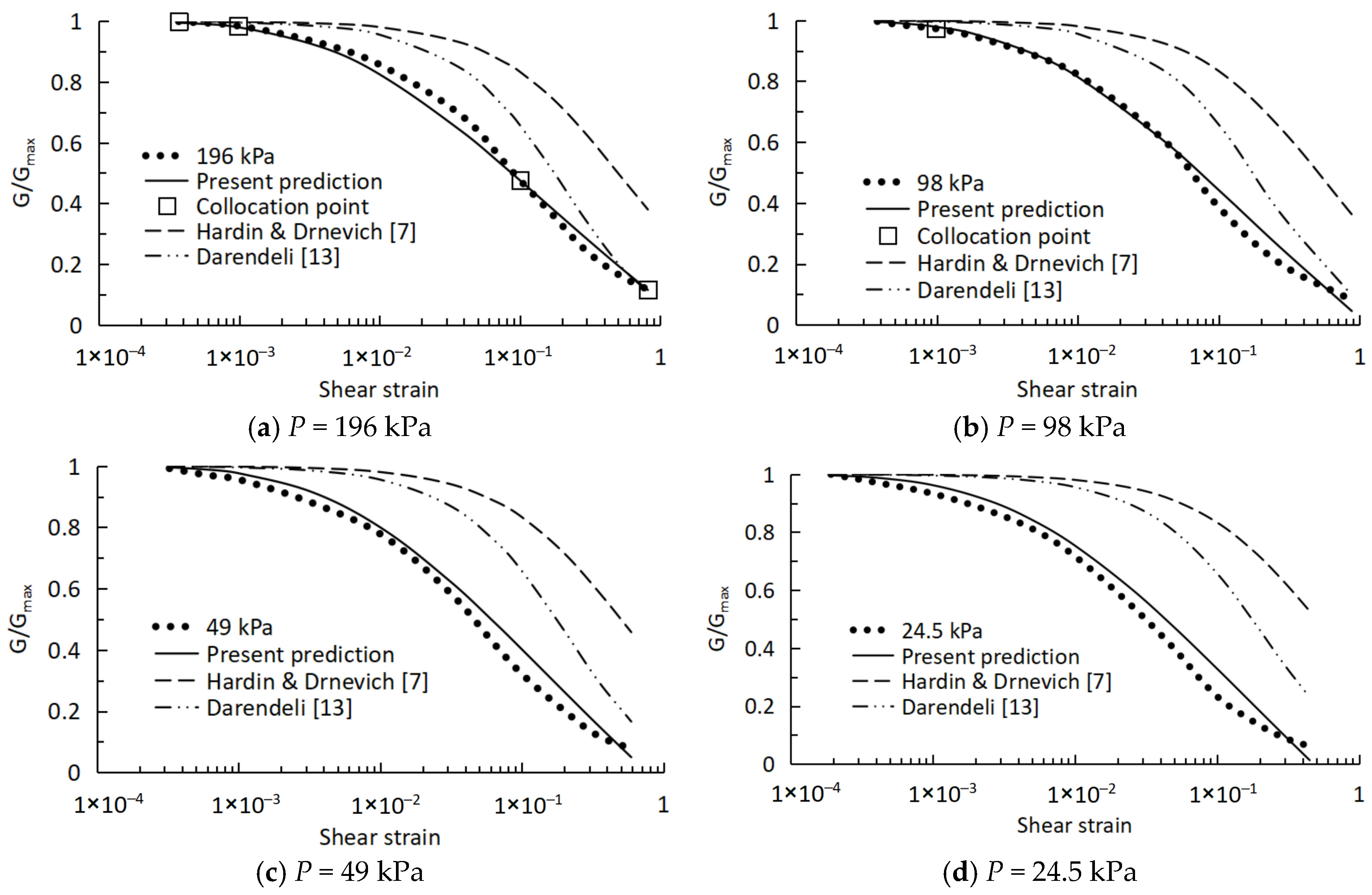
The modulus over a wide strain range (γ = 10⁻⁴–10^–1) was obtained in Iwasaki et al. [28] for Toyoura sand by combining the RC and TCS results. The effects of confining pressure were tested for P = 24.5, 49, 98, and 196 kPa. The normalized $G/G_{max}$ curves are plotted in Figure 1 as functions of the shear strain defined by Equation (19), together with the experimental data and the models [7,13] under different confining pressures. The parameters C₁ = −0.2722, C₂ = −0.1701, D₁ = −0.6144, D₂ = 0.02596, and D = 0.00012 were obtained from the least-squares fitting (P in kPa for all curves hereafter). Figure 1 shows that the calculated curves agree well with the experimental data.

The local logarithmic form of Equation (19) for $1-G/G_{max}$ is

$$\mathrm{l}\mathrm{n}\left(1-{\displaystyle \frac{G}{G_{max}}}\right)\approx D_1{\mathsf{\gamma }\left(t\right)}^{C_1}+D_2{P\left(t\right)}^{C_2}+D.$$

(20)

Then the local sensitivity of the parameters is

$$\left\{\begin{array}{c}{\displaystyle \frac{\partial \mathrm{l}\mathrm{n}\left(1-\frac{G}{G_{max}}\right)}{\partial \mathrm{l}\mathrm{n}\left(D_1\right)}}=-0.6144{\mathsf{\gamma }\left(t\right)}^{-0.2722}\\ {\displaystyle \frac{\partial \mathrm{l}\mathrm{n}\left(1-\frac{G}{G_{max}}\right)}{\partial \mathrm{l}\mathrm{n}\left(D_2\right)}}=0.02596{\mathsf{\gamma }\left(t\right)}^{-0.1701}\\ {\displaystyle \frac{\partial \mathrm{l}\mathrm{n}\left(1-\frac{G}{G_{max}}\right)}{\partial \mathrm{l}\mathrm{n}\left(C_1\right)}}=0.1672{\mathsf{\gamma }\left(t\right)}^{-0.2722}\mathrm{l}\mathrm{n}\left(\mathsf{\gamma }\left(t\right)\right)\\ {\displaystyle \frac{\partial \mathrm{l}\mathrm{n}\left(1-\frac{G}{G_{max}}\right)}{\partial \mathrm{l}\mathrm{n}\left(C_2\right)}}=-0.004415{\mathsf{\gamma }\left(t\right)}^{-0.1701}\mathrm{l}\mathrm{n}\left(\mathsf{\gamma }\left(t\right)\right)\\ {\displaystyle \frac{\partial \mathrm{l}\mathrm{n}\left(1-\frac{G}{G_{max}}\right)}{\partial \mathrm{l}\mathrm{n}\left(D\right)}}=0.00012\end{array}\right..$$

(21)

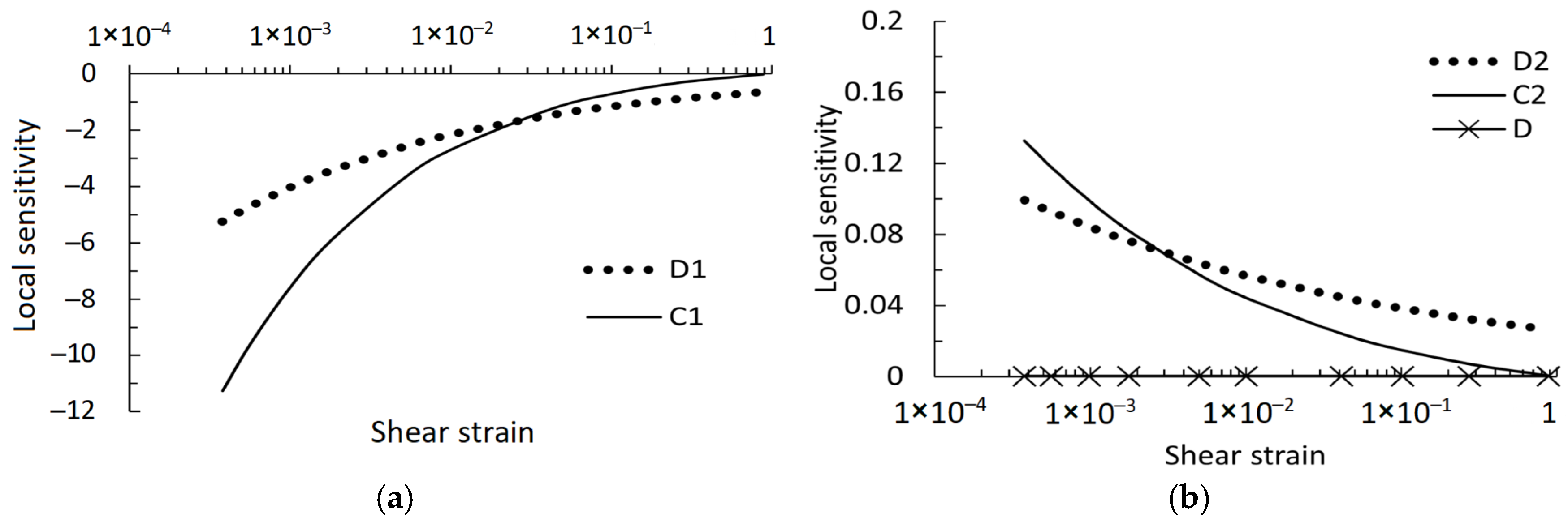
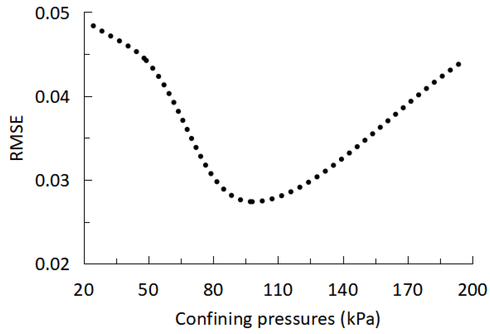
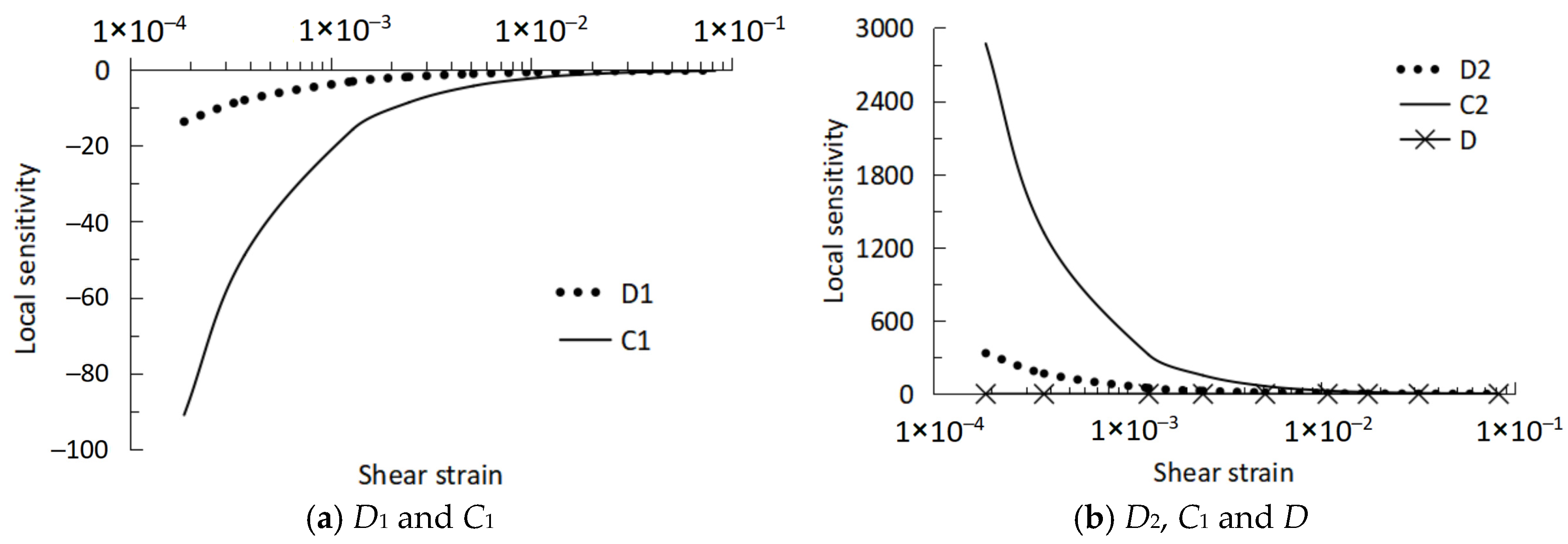
To further evaluate the influence of model parameters, a local sensitivity analysis was performed for Toyoura sand, as shown in Figure 2. Figure 2a indicates that parameter C₁ exerts the dominant influence at relatively small strain levels, whereas the effect of D₁ becomes more pronounced as the shear strain increases. Figure 2b shows that D₂ and C₂ have comparatively smaller but still non-negligible effects, while parameter D remains only weakly influential over the strain range considered. In addition, we provide the root mean square error (RMSE) for the present prediction and the experimental results in Figure 3 for different confining pressures. The RMSE value first decreases from 0.0483 in 24.5 kPa to 0.0274 in 98 kPa, and it then increases to 0.0442 in 196 kPa. The maximum value of RMSE occurred in 24.5 kPa pressure. These results suggest that different parameters govern the shape of the modulus-reduction curve in different strain intervals.

3.2. Validation Against the Experimental Data of Zhu et al. [29]

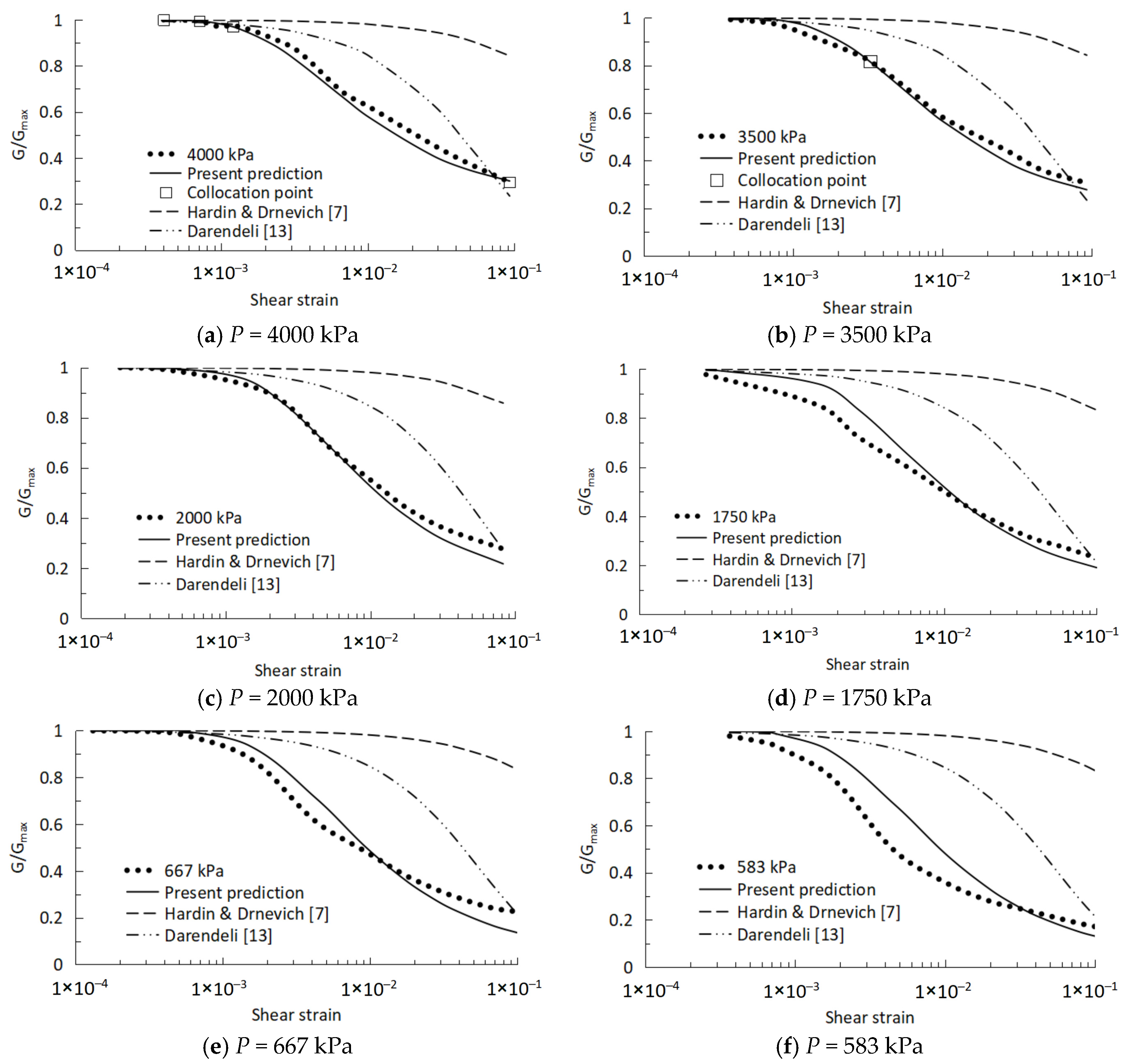
The normalized $G/G_{\mathrm{m}\mathrm{a}\mathrm{x}}$ curves of gravels under high confining pressures ($P=667$ kPa, 1750 kPa, 2000 kPa, 3500 kPa, and 4000 kPa) were measured by Zhu et al. [29]. The shear strain varies from 0.0005 to 0.1. The fitted parameters are $C_1=-0.7762$, $C_2=1.001$, $D_1=-0.017398$, $D_2=0.06168$, and $D=0.000021$. Figure 4 compares the present prediction with the experimental data as well as the existing models [7,13] under different confining pressures. Satisfactory agreement is observed in Figure 4a–c, whereas some deviations appear in Figure 4d–f around $1.00\times {10}^{-3}$. This deviation may be attributed to the fact that the collocation points were selected from the curves in panels a and b, whereas the curve in panel f exhibits a different shape.

Meanwhile, the local sensitivity of the parameters is

$$\left\{\begin{array}{c}{\displaystyle \frac{\partial \mathrm{l}\mathrm{n}\left(1-\frac{G}{G_{max}}\right)}{\partial \mathrm{l}\mathrm{n}\left(D_1\right)}}=-0.017398{\mathsf{\gamma }\left(t\right)}^{-0.7762}\\ {\displaystyle \frac{\partial \mathrm{l}\mathrm{n}\left(1-\frac{G}{G_{max}}\right)}{\partial \mathrm{l}\mathrm{n}\left(D_2\right)}}=0.06168{\mathsf{\gamma }\left(t\right)}^{-1.001}\\ {\displaystyle \frac{\partial \mathrm{l}\mathrm{n}\left(1-\frac{G}{G_{max}}\right)}{\partial \mathrm{l}\mathrm{n}\left(C_1\right)}}=0.0135{\mathsf{\gamma }\left(t\right)}^{-0.7762}\mathrm{l}\mathrm{n}\left(\mathsf{\gamma }\left(t\right)\right)\\ {\displaystyle \frac{\partial \mathrm{l}\mathrm{n}\left(1-\frac{G}{G_{max}}\right)}{\partial \mathrm{l}\mathrm{n}\left(C_2\right)}}=-0.06174{\mathsf{\gamma }\left(t\right)}^{-1.001}\mathrm{l}\mathrm{n}\left(\mathsf{\gamma }\left(t\right)\right)\\ {\displaystyle \frac{\partial \mathrm{l}\mathrm{n}\left(1-\frac{G}{G_{max}}\right)}{\partial \mathrm{l}\mathrm{n}\left(D\right)}}=0.000021\end{array}\right..$$

(22)

In Figure 5, we show the local sensitivity of the parameters in the strain range (γ = 0.05–1%). The parameter C₂ has the greatest influence on the model.

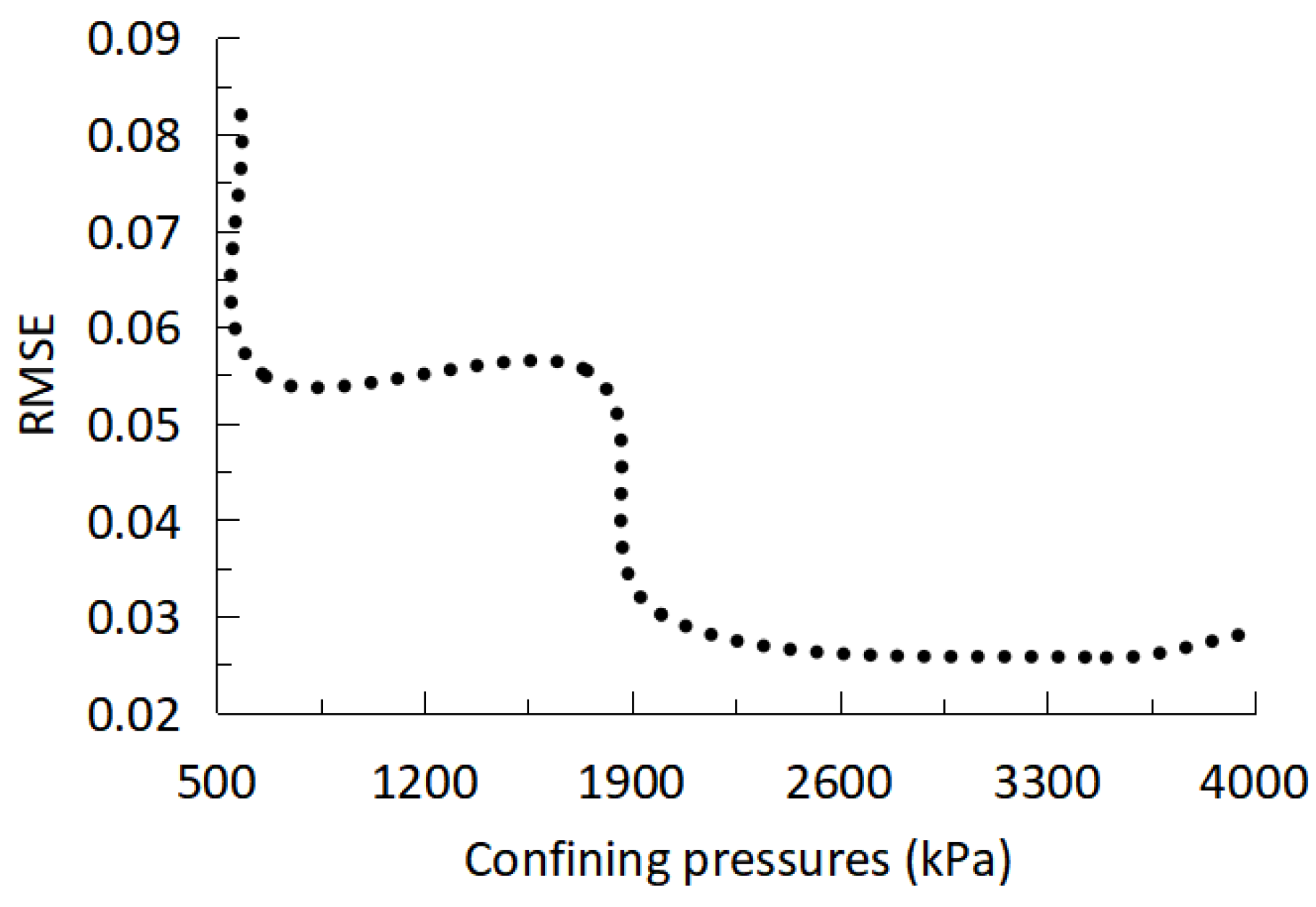
We also provide the RMSE for the present prediction and the experimental results in Figure 6 for different confining pressures. The RMSE value first decreases from 0.08198 in 583 kPa to 0.0554 in 1750 kPa, then decreases to 0.0257 in 3500 kPa, and at last increases to 0.02836 in 4000 kPa. The maximum value of RMSE occurred in 583 kPa pressure.

4. Application

4.1. Slope Stability Analysis and Comparison with Conventional Results

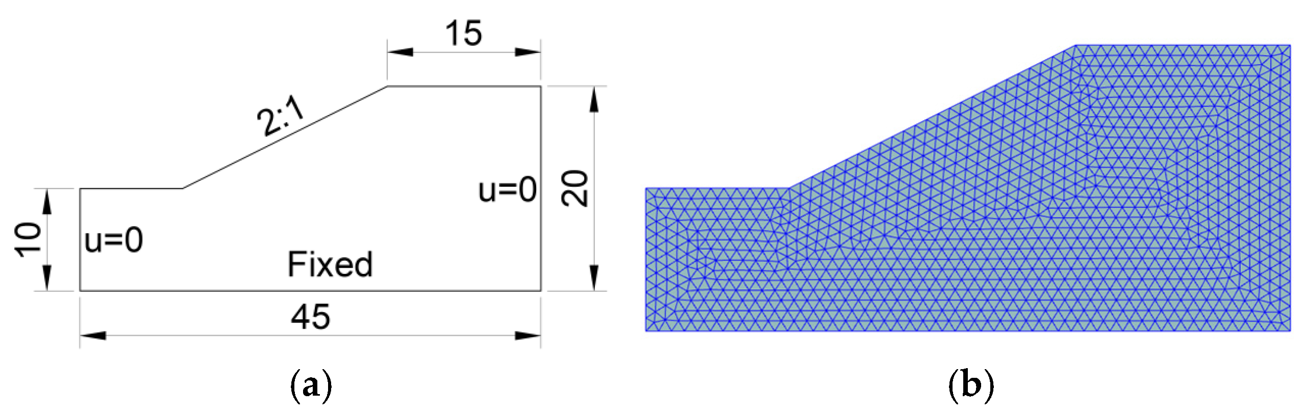
In this section, the material model introduced in Section 2 is applied to the slope stability analysis. The slope geometry and finite-element discretization are built by finite element software COMSOL Multiphysics 6.3 in Figure 7.

In Figure 7, there are 2241 domain units and 137 boundary units. The shear modulus G_max = 9 × 10⁷ Pa, Poisson’s ratio is $\nu =0.4$, and the shear modulus $G$ is taken from the experiment of Zhu et al. [29] as

$$G=G_{max}\left(1-e^{-0.017398{\gamma }^{-0.7762}-6.126\times {10}^{-5}{P}^{1.0002}+0.00021}\right).$$

(23)

The density of the soil is 2000 kg/m³. By the Morgenstern–Price method (Jiang and Yamagami [30]), the pore water pressure distribution coefficient $r_u$ is

$$r_u={\displaystyle \frac{P}{{\gamma }^{\prime }h}},$$

(24)

in which ${\gamma }^{\prime }$ is the bulk density of the soil, and $h$ is the depth of the point in the soil mass below the soil surface. The Mohr–Coulomb criterion implemented in COMSOL Multiphysics is expressed as follows [32]:

$${\displaystyle \frac{1}{2}}\left({\sigma }_1-{\sigma }_3\right)+{\displaystyle \frac{1}{2}}\left({\sigma }_1+{\sigma }_3\right)\mathrm{s}\mathrm{i}\mathrm{n}{\varphi }^{\prime }-c^{\prime }\mathrm{c}\mathrm{o}\mathrm{s}{\varphi }^{\prime }=0,$$

(25)

where ${\sigma }_1$ and ${\sigma }_3$ are the first and third principal stresses, ${\varphi }^{\prime }$ is the friction angle, and $c^{\prime }$ is the shear strength. The yield function $F_y$ has a hexagonal octahedral section [32], and it is written as

$$F_y=\mathsf{\Gamma }\left(\theta \right){\sigma }_{\mathrm{m}\mathrm{i}\mathrm{s}\mathrm{e}\mathrm{s}}+\alpha {\sigma }_{\mathrm{m}}-k,$$

(26)

in which $\mathsf{\Gamma }\left(\theta \right)$ is a function of the Lode angle $\theta$ that defines the shape of the yield function in the octahedral plane. The most common choice is $\mathsf{\Gamma }\left(\theta \right)=1$. Similarly, ${\sigma }_{\mathrm{m}\mathrm{i}\mathrm{s}\mathrm{e}\mathrm{s}}$ is the Mises stress, ${\sigma }_{\mathrm{m}}$ is the mean stress, and $\alpha$ and $k$ are [32]

$$\left\{\begin{array}{c}\alpha ={\displaystyle \frac{6\mathrm{s}\mathrm{i}\mathrm{n}{\varphi }^{\prime }}{3-\mathrm{s}\mathrm{i}\mathrm{n}{\varphi }^{\prime }}}\\ k=c^{\prime }{\displaystyle \frac{6\mathrm{s}\mathrm{i}\mathrm{n}{\varphi }^{\prime }}{3-\mathrm{s}\mathrm{i}\mathrm{n}{\varphi }^{\prime }}}\end{array}\right..$$

(27)

According to Equation (1), the effective stress tensor component ${\sigma }_{ij}$ can be expressed as

$${\sigma }_{ij}=\left(1-{\varphi }^2\right)\left[\left(1-\phi \right){\mathbb{C}}_{ijlk}{\mathsf{\epsilon }}_{ij}-\phi {\alpha }_B{\delta }_{ij}P\right].$$

(28)

When the pressure distribution coefficient $r_u$ is given, the pressure $P$ is a function of the depth of the point in the soil h. The strain tensor component ${\mathsf{\epsilon }}_{ij}$ is expressed as

$${\mathsf{\epsilon }}_{ij}={\mathsf{\epsilon }}_{eij}+{\mathsf{\epsilon }}_{pij},$$

(29)

in which ${\mathsf{\epsilon }}_{eij}$ and ${\mathsf{\epsilon }}_{pij}$ are the strain tensors induced by elastic and plastic deformations. COMSOL Multiphysics characterizes plastic deformation through the plastic strain tensor component coupled with the Mohr–Coulomb yield function as [32]

$${\mathsf{\epsilon }}_{\mathit{p}}=\lambda {\displaystyle \frac{\partial F_y}{\partial \mathit{\sigma }}},$$

(30)

where $\lambda$ is the plastic multiplier, $\mathit{\sigma }$ is the total stress tensor, and the von Mises equivalent plastic strain is [32]

$${\mathsf{\epsilon }}_{pe}=\sqrt{{\displaystyle \frac{2}{3}}{\mathsf{\epsilon }}_{\mathit{p}}:{\mathsf{\epsilon }}_{\mathit{p}}}$$

(31)

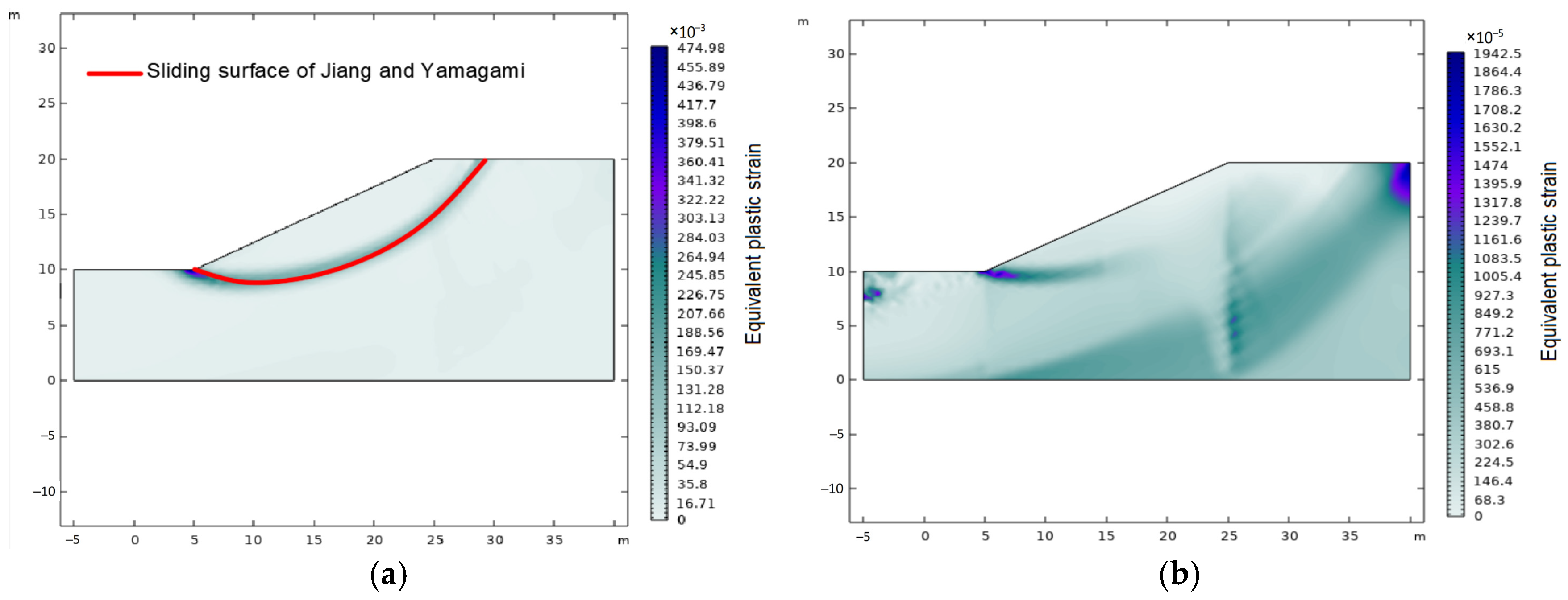
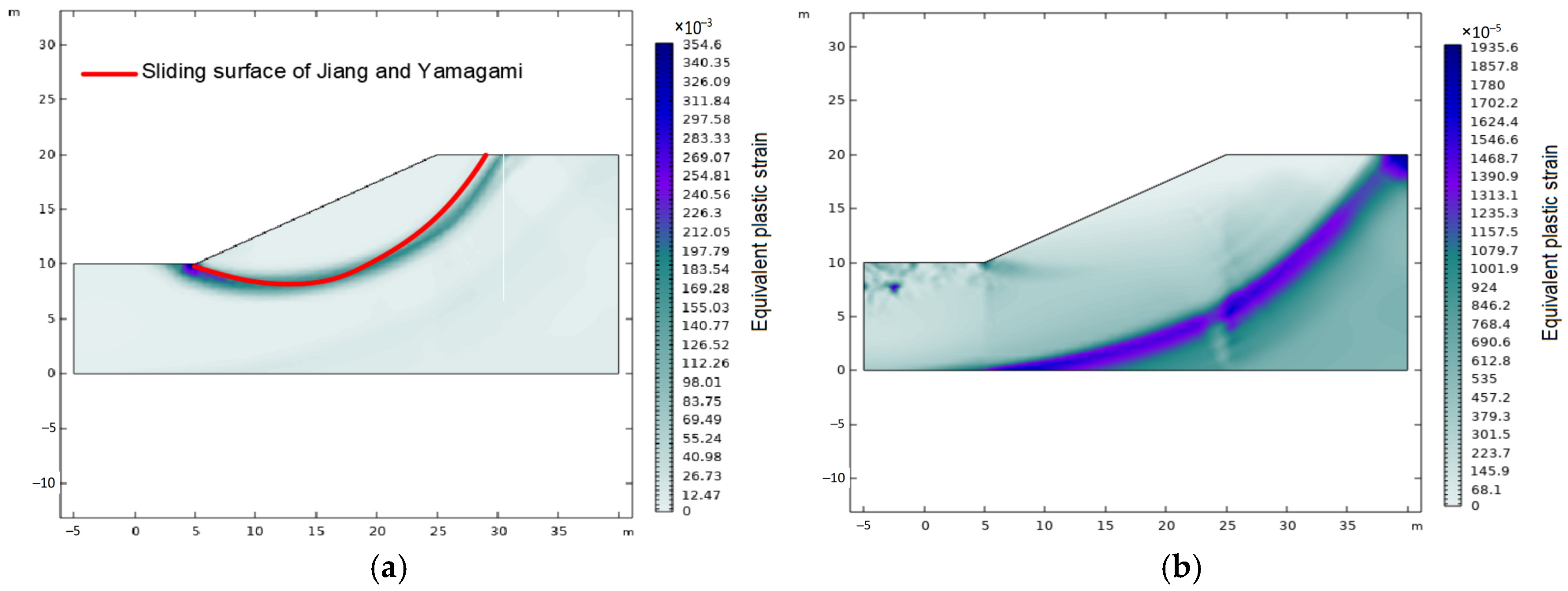
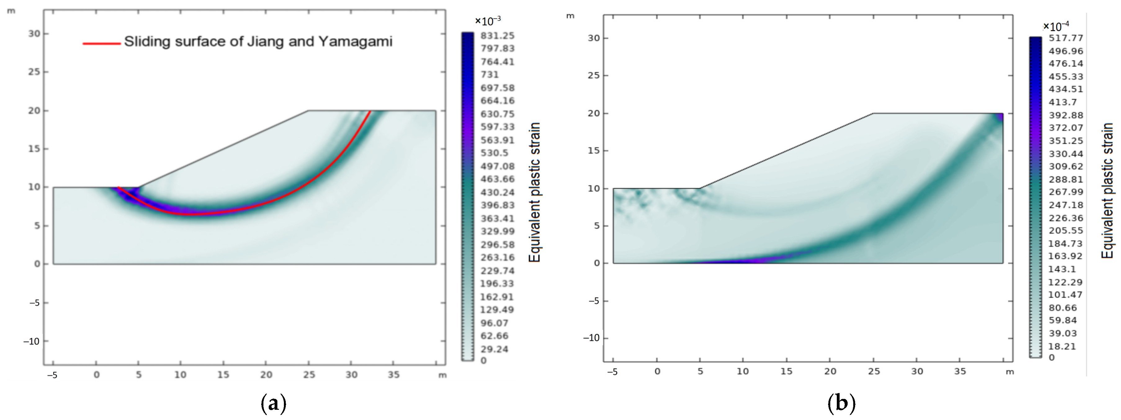
${\mathsf{\epsilon }}_{\mathit{p}}$ is the plastic strain tensor. According to Jiang and Yamagami [30], $r_u$ = 0.25, and the plastic deformation is assumed to follow the Mohr–Coulomb criterion. The strength reduction method was applied [30], and three plastic zones were calculated with shear strength $c^{\prime }$ = 9.96 kN/m², 15.22 kN/m², and 19.2 kN/m² and friction angle ${\varphi }^{\prime }$ = 15.8°, 9.8°, and 6.2° for F = 1 in Figure 8, Figure 9 and Figure 10.

As shown in Figure 8, Figure 9 and Figure 10, the potential sliding surface is located in the vicinity of the maximum plastic-potential zone, extending from the slope toe to a region within approximately 6 m of the slope crest. With an increase in shear strength and a decrease in friction angle, the potential sliding surface tends to move farther away from the slope crest. In the case without confining pressure, the predicted plastic-zone distribution is generally consistent with the sliding-surface pattern reported by Jiang and Yamagami [30]. The equivalent strain thresholds of failure planes in the present predictions are 460 × 10⁻³, 350 × 10⁻³, and 800 × 10⁻³ for Figure 8, Figure 9 and Figure 10 without confining pressure, respectively. As the plastic equivalent strain exceeds these thresholds, it is considered that the soil has been damaged, resulting in the formation of a slip surface. When confining pressure is considered, the plastic zone becomes noticeably larger and extends further toward the crest region. This trend can be interpreted as a consequence of stiffness degradation associated with increasing pore-pressure effects at greater depth, which leads to larger deformation and a broader potential sliding region. These results suggest that the proposed model may provide a useful framework for assessing failure zones in embankments, retaining structures, and harbor slopes.

4.2. Discussion and Engineering Implications

The present results indicate that the introduction of confining pressure affects slope stability not only through stress redistribution but also through the degradation of soil and gravel stiffness represented by the shear modulus. In the proposed framework, this degradation leads to a wider plastic zone and a larger potential sliding region, suggesting that the effect may become more significant in saturated slopes subjected to strong confinement variation or seismic loading. From an engineering perspective, this mechanism is relevant to the stability assessment of embankments, retaining structures, and harbor slopes, where conventional analyses based solely on fixed material parameters may underestimate the extent of potential failure zones. However, the current model remains simplified in that it does not explicitly include clay damage, soil yield-stress evolution, or more comprehensive drainage conditions effects, and these issues should be investigated in future studies.

5. Conclusions

In this study, a generalized constitutive relationship among shear strain, confining pressure, and shear modulus was established within a phase-field framework based on the Günzburg–Landau equation. Our conclusions are as follows:

(1)

A new shear modulus coupled with shear strain and confining pressure is proposed based on a phase-field method.

By introducing an order parameter to characterize stiffness degradation under variable confining pressure, the proposed model provides a physically interpretable description of the modulus-reduction process and is intended to be applicable to sand and gravel, but not to clay yet. Validation against published test data with the strain belonging to 10⁻⁴–10^–1, together with comparisons with existing models, shows that the present model can reasonably capture the influence of confining pressure on the normalized shear modulus over a wide range of strain levels.

(2)

The dominant sensitivity parameters of the present model are identified for sand and gravel.

The local sensitivity analysis further indicates that different parameters dominate the response in different strain ranges, which helps clarify the role of model parameters in controlling 1 − G/G_max. In the present model (19) and validated examples, the parameter C₁ exerts the dominant influence for sand shear modulus damage, and the parameter C₂ has the greatest influence on gravel.

(3)

The present model is used to analyze the slope instability for engineering application.

Application to saturated slope stability analysis shows that confining pressure can significantly enlarge the plastic zone and alter the potential sliding-surface pattern; the predicted distribution is also broadly consistent with the tendency reported by Jiang and Yamagami [30]. These results suggest that confining-pressure-induced stiffness degradation should not be neglected in practical assessments of embankments, retaining structures, and harbor slopes. Nevertheless, the present study does not explicitly consider the effect of yield stress or more complex hydro-mechanical coupling, and further validation against additional soils and engineering cases is still needed. These aspects will be addressed in future work.

References

1. Seed, H.B. The fourth Terzaghi lecture: Landslides during earthquakes due to liquefaction. J. Soil Mech. Found. Div. 1968, 94, 1053–1122. [Google Scholar] [CrossRef]
2. Prakash, S.; Puri, V.K. Dynamic properties of soils from in-situ tests. J. Geotech. Eng. Div. 1981, 107, 943–964. [Google Scholar] [CrossRef]
3. Seed, H.B.; Wong, R.T.; Idriss, I.M.; Tokimatsu, K. Moduli and damping factors for dynamic analyses of cohesionless soils. J. Geotech. Eng. 1986, 112, 1016–1032. [Google Scholar] [CrossRef]
4. Oztoprak, S.; Bolton, M.D. Stiffness of sands through a laboratory test database. Géotechnique 2013, 63, 54–70. [Google Scholar] [CrossRef]
5. Anderson, D.G.; Richart, F.E. Effects of straining on shear modulus of clays. J. Geotech. Eng. Div. 1976, 102, 975–987. [Google Scholar] [CrossRef]
6. Hardin, B.O.; Black, W.L. Sand stiffness under various triaxial stresses. J. Soil Mech. Found. Div. 1966, 92, 27–42. [Google Scholar] [CrossRef]
7. Hardin, B.O.; Drnevich, V.P. Shear modulus and damping in soils: Measurement and parameter effects. J. Soil Mech. Found. Div. 1972, 98, 603–624. [Google Scholar] [CrossRef]
8. Seed, H.B.; Idriss, I.M. Simplified procedure for evaluating soil liquefaction potential. J. Soil Mech. Found. Div. 1971, 97, 1249–1273. [Google Scholar] [CrossRef]
9. Sherif, M.A.; Ishibashi, I.; Cheng, W.L. Soil parameters affecting pore-pressure buildup during earthquakes. J. Geotech. Eng. Div. 1976, 102, 1171–1184. [Google Scholar] [CrossRef]
10. Khouri, N.Q. Dynamic Properties of Soils. Master’s Thesis, Syracuse University, Syracuse, NY, USA, 1984. [Google Scholar]
11. Ishibashi, I.; Zhang, X. Unified dynamic shear moduli and damping ratios of sand and clay. Soils Found. 1993, 33, 182–191. [Google Scholar] [CrossRef]
12. Alarcon-Guzman, A.; Chameau, J.L.; Leonards, G.A.; Frost, J.D. Shear modulus and cyclic undrained behavior of sands. Soils Found. 1989, 29, 105–119. [Google Scholar] [CrossRef]
13. Darendeli, M.B. Development of a New Family of Normalized Modulus Reduction and Material Damping Curves. Ph.D. Thesis, The University of Texas at Austin, Austin, TX, USA, 2001. [Google Scholar]
14. Collins, I.F.; Houlsby, G.T. Application of thermomechanical principles to the modelling of geotechnical materials. Proc. R. Soc. Lond. A 1997, 453, 1975–2001. [Google Scholar] [CrossRef]
15. Collins, I.F.; Kelly, P.A. A thermomechanical analysis of a family of soil models. Géotechnique 2002, 52, 507–518. [Google Scholar] [CrossRef]
16. Collins, I.F.; Hilder, T. A theoretical framework for constructing elastic/plastic constitutive models of triaxial tests. Int. J. Numer. Anal. Methods Geomech. 2002, 26, 1313–1347. [Google Scholar] [CrossRef]
17. Jiang, Y.M.; Liu, M. Granular solid hydrodynamics. Granul. Matter 2009, 11, 139–156. [Google Scholar] [CrossRef]
18. Xiao, Y.F.; Liang, F.; Zhang, Z.C.; Wu, H.R.; Liu, H.L. Thermodynamic constitutive model for granular soils considering particle shape distribution. Comput. Geotech. 2023, 162, 105700. [Google Scholar] [CrossRef]
19. Zhang, Z.C.; Cheng, X.H. Effective stress in saturated soil: A granular solid hydrodynamics approach. Granul. Matter 2014, 16, 761–769. [Google Scholar] [CrossRef]
20. Jiang, Y.; Einav, I.; Liu, M. A thermodynamic treatment of partially saturated soils revealing the structure of effective stress. J. Mech. Phys. Solids 2017, 100, 131–146. [Google Scholar] [CrossRef]
21. Xiao, Y.; Wang, C.G.; Zhang, Z.C.; Liu, H.L.; Yin, Z.Y. Constitutive modeling for two sands under high pressure. Int. J. Geomech. 2021, 21, 04021042. [Google Scholar] [CrossRef]
22. Baturina, T.I.; Vinokur, V.M. Ginzburg–Landau equations. In 100 Years of Superconductivity; Rogalla, H., Kes, P.H., Eds.; CRC Press: Boca Raton, FL, USA, 2011; pp. 51–65. [Google Scholar] [CrossRef]
23. Yang, S. Phase-Field Modeling for Self-Healing of Mineral-Based Materials. Doctoral Dissertation, Technische Universität Darmstadt, Darmstadt, Germany, 2021. [Google Scholar]
24. Ginzburg, V.L.; Landau, L.D. On the theory of superconductivity. Zh. Eksp. Teor. Fiz. 1950, 20, 1064–1073. [Google Scholar]
25. Choo, J.; Sun, W. Coupled phase-field and plasticity modeling of geological materials: From brittle fracture to ductile flow. Comput. Methods Appl. Mech. Eng. 2018, 330, 1–32. [Google Scholar] [CrossRef]
26. Gavagnin, C.; Sanavia, L.; De Lorenzis, L. Stabilized mixed formulation for phase-field computation of deviatoric fracture in elastic and poroelastic materials. Comput. Mech. 2020, 65, 1447–1465. [Google Scholar] [CrossRef]
27. Schneider, D.; Schoof, E.; Tschukin, O.; Reiter, A.; Herrmann, C.; Schwab, F.; Selzer, M.; Nestler, B. Small-strain multiphase-field model accounting for configurational forces and mechanical jump conditions. Comput. Mech. 2018, 61, 277–295. [Google Scholar] [CrossRef]
28. Iwasaki, T.; Tatsuoka, F.; Takagi, Y. Dynamic Shear Deformation Properties of Sand for Wide Strain Range; Report of Civil Engineering Institute, No. 1085; Ministry of Construction: Tokyo, Japan, 1976. [Google Scholar]
29. Zhu, S.; Yang, G.; Wen, Y.; Ou, L. Dynamic shear modulus reduction and damping under high confining pressures for gravels. Geotech. Lett. 2014, 4, 179–186. [Google Scholar] [CrossRef]
30. Jiang, C.J.; Yamagami, T. Charts for estimating strength parameters from slips in homogeneous slopes. Comput. Geotech. 2006, 33, 294–304. [Google Scholar] [CrossRef]
31. Yuan, Y.; Sang, Q.Z.; Chen, X. Dynamic shear modulus degradation of saturated soil analysis: From the perspective of phase field theory. Comput. Struct. 2024, 305, 107568. [Google Scholar] [CrossRef]
32. COMSOL AB. Structural Mechanics Module User’s Guide, COMSOL Multiphysics® v. 6.4; COMSOL AB: Stockholm, Sweden, 2026; Available online: https://doc.comsol.com/6.4/docserver/#!/com.comsol.help.comsol/helpdesk/helpdesk.html (accessed on 15 March 2026).
Figure 1. Normalized G / G m a x curves versus shear strain for Toyoura sand under different confining pressures. The present prediction, the Hardin & Drnevich model, the Darendeli model [7,13], the collocation points, and the experimental data are shown.
Applsci 16 05003 g001
Figure 2. Local sensitivity of the normalized 1 G / G m a x response with respect to model parameters for Toyoura sand: (a) D1 and C1; (b) D2, C2, and D.
Applsci 16 05003 g002
Figure 3. The RMSE between the present prediction and Toyoura sand under different confining pressures.
Applsci 16 05003 g003
Figure 4. Normalized G / G m a x curves versus shear strain for gravels under different confining pressures. The present prediction, the Hardin & Drnevich model, the Darendeli model [7,13], the collocation points, and the experimental data are shown for (a) P = 4000 kPa; (b) P = 3500 kPa; (c) P = 2000 kPa; (d) P = 1750 kPa; (e) P = 667 kPa; and (f) P = 583 kPa.
Applsci 16 05003 g004
Figure 5. Local sensitivity of the 1 − G/Gmax curves with respect to shear strain.
Applsci 16 05003 g005
Figure 6. The RMSE between the present prediction and experimental data for gravels under different confining pressures.
Applsci 16 05003 g006
Figure 7. Slope geometry and finite-element discretization (Unit: m): (a) geometric; (b) unit division.
Applsci 16 05003 g007
Figure 8. The plastic zone with and without confining pressure in c′ = 9.96 kN/m2, ϕ′ = 15.8°: (a) without confining pressure; (b) with confining pressure.
Applsci 16 05003 g008
Figure 9. The plastic zone with and without confining pressure in c′ = 15.22 kN/m2, ϕ′ = 9.8°: (a) without confining pressure; (b) with confining pressure.
Applsci 16 05003 g009
Figure 10. The plastic zone with and without confining pressure in c′ = 19.2 kN/m2, ϕ′ = 6.2°: (a) without confining pressure; (b) with confining pressure.
Applsci 16 05003 g010
Disclaimer/Publisher’s Note: The statements, opinions and data contained in all publications are solely those of the individual author(s) and contributor(s) and not of MDPI and/or the editor(s). MDPI and/or the editor(s) disclaim responsibility for any injury to people or property resulting from any ideas, methods, instructions or products referred to in the content.