Dynamic p-y Model for Laterally Loaded Piles near Clay Slope

Abstract

Seismic loading can significantly affect the safety and serviceability of structures supported by piles, making seismic performance a key consideration in pile foundation design. The coupling between slope effect and dynamic loading can significantly alter pile–soil interaction and consequently influence the response of laterally loaded piles. In the present study, a dynamic extension of the static p-y curve model for piles near clay slopes is developed for analyzing the response of laterally loaded piles under dynamic loading, based on adjustment of the real stiffness component, and the spring and dashpot model. A computational program based on the Beam on Dynamic Winkler Foundation (BDWF) model is developed for analyzing the dynamic response of piles near a slope. Comparison with finite element simulation results shows that the complex stiffness scheme provides accurate response predictions, thereby validating the effectiveness of the proposed model. Finally, parametric analyses are carried out to investigate the effects of loading parameters (excitation frequency and load amplitude), pile parameters (pile diameter, pile length, and adhesion coefficient), boundary conditions (pile-head and pile-tip constraints), and slope parameter (slope angle). The pile–soil system exhibits a characteristic frequency governed by the soil shear-wave velocity and pile diameter, while being essentially independent of slope angle and pile length. Near this frequency, the pile-head stiffness and damping ratio change significantly. The proposed method provides a practical tool for steady-state dynamic analysis of laterally loaded piles near clay slopes.

1. Introduction

Slope stability is a fundamental concern in geotechnical engineering, because it directly affects the safety and serviceability of engineering systems constructed on or near sloping ground. In practical projects, changes in geological conditions, slope geometry, and external disturbances may alter the stability state of the slope and further influence the performance of adjacent structures and foundations [1,2,3].

For pile foundations constructed near slopes, dynamic loads induced by earthquakes, waves, and mechanical vibrations are common design conditions and often play a controlling role [4,5]. Compared with flat ground, the bearing capacity of laterally loaded piles in complex topographies, such as mountainous and coastal areas, is affected by the slope effect [6,7,8,9].

The p-y curve model is widely adopted as a practical and effective approach for investigating slope effect [9,10,11,12]. This method idealizes the soil around the pile as a series of nonlinear springs represented by p-y curves. Based on experimental studies [13,14], numerical analyses [11,12] and theoretical studies [8,9], static p-y curve models applicable to piles near slope have been developed and improved. However, these models do not account for inertial effects or vibration propagation and dissipation within the pile–soil system, making them unsuitable for directly predicting the dynamic response of piles near a slope.

Previous researchers have conducted theoretical studies in the frequency domain on dynamic pile–soil interactions using the plane strain model [15,16,17], the three-dimensional elastic continuum model [18] and the damped complex stiffness three-dimensional viscoelastic model [4,5,19,20]. These studies have produced a series of frequency-dependent analytical solutions for soil resistance. However, due to the complexity of the models, the above-mentioned methods rely on the assumption of a semi-infinite space, which restricts their applicability to slopes. Some researchers have applied the wave field extrapolation (WFE) method to calculate the dynamic response of piles near slopes under SH seismic waves [21,22,23]. This approach accounts for the topographic amplification of free-field displacements, but fails to capture the effect of the slope on the stiffness of the soil surrounding the pile. In addition, some researchers have proposed dynamic correction methods for static p-y curve models to account for dynamic response. These methods were developed by combining model-test results with fitted results derived from the hyperbolic stress–strain model, leading to two representative approaches, namely adjustment of the real stiffness component, and the spring and dashpot model [24,25]. These methods are developed within an equivalent linear framework based on representative soil parameters, and do not explicitly account for strain-dependent modulus degradation, cyclic degradation, or progressive soil plasticity under repeated loading.

These methods provide a practical way to represent the variation in soil resistance with loading frequency and to carry out equivalent linear analyses of transient pile response. However, they were mainly developed for level ground. Under that condition, the p-y relationship does not reflect the reduction in soil resistance caused by the slope effect. For piles near slopes, the initial stiffness, the ultimate soil resistance, and the soil flow mechanism near the ground surface are all affected by the presence of the slope.

This study presents a computational method for evaluating the dynamic response of laterally loaded piles near slopes. The proposed method extends the existing static p-y curve formulation for slope conditions to dynamic loading by incorporating two dynamic correction approaches, namely adjustment of the real stiffness component, and the spring and dashpot model. Based on the resulting dynamic p-y relationship, pile responses, including lateral displacement and bending moment along the pile shaft, are calculated using the Beam on Dynamic Winkler Foundation (BDWF) model. To assess the validity of the proposed method, the results are compared with those from three-dimensional numerical simulations. The comparisons show that the proposed method can reasonably predict the dynamic response of laterally loaded piles near slopes. Furthermore, parametric analyses are carried out to investigate the effects of loading parameters, pile parameters, and slope parameters. The proposed method is expected to provide a practical tool for analyzing the steady-state dynamic response of single laterally loaded piles near clay slopes, and to offer useful support for preliminary design, parametric evaluation, and engineering assessment.

2. Theoretical Model

2.1. Problem Definition

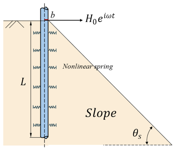
As shown in Figure 1, the pile is modeled with the following properties: length $L$, diameter $D$, mass density ${\rho }_p$, cross-sectional area $A_p$, Young’s modulus $E_p$ and section modulus $I_p$. Both the pile top and pile tip are free, with no constraints applied. The slope angle is denoted as ${\theta }_s$, and the near-slope distance is denoted as $b$ (i.e., distance from the centerline of the pile to the slope crest). The present formulation follows the idealized slope geometry adopted in the underlying static slope p-y model and does not explicitly include slope height as an independent variable. Therefore, slope height is not treated as an independent parameter in this study. The pile top is subjected to a horizontal dynamic load with an amplitude of $H_0$ and a frequency of $\omega$, represented by $H_0{e}^{i\omega t}$. The pile is surrounded by clay, which is characterized by the following parameters: Young’s modulus $E_s$, Poisson’s ratio $\upsilon$, shear modulus $G_s=E_s/\left[2\right(1+\upsilon \left)\right]$, soil density ${\rho }_s$, and undrained shear strength $c_u$.

2.2. Dynamic p-y Curve Model

In this section, the static p-y curve for piles near slopes is extended to dynamic loading conditions. Previous test results for laterally loaded piles in clay under flat-ground conditions indicate that the undrained static p-y curve can be represented by a hyperbolic equation [26,27,28]:

$$p_{s\theta }={\displaystyle \frac{y}{\left(\frac{1}{k_{i\theta }}\right)+\left(\frac{y}{p_{u\theta }}\right)}}$$

(1)

where $p_{s\theta }$, $k_{i\theta }$, and $p_{u\theta }$ denote the static soil resistance, initial stiffness, and ultimate soil resistance under slope conditions, respectively, and $y$ indicates the soil displacement. For laterally loaded piles, the initial soil stiffness $k_i$ is obtained from Equation (2) [29]:

$$k_i={\displaystyle \frac{1.3E_s}{1-{\nu }^2}}{\left({\displaystyle \frac{E_s{D}^4}{E_p{I}_p}}\right)}^{{\displaystyle \frac{1}{12}}}$$

(2)

Considering the presence of slopes within the depth range of $0$ to $6D$, the initial soil stiffness is reduced by a factor associated with the slope angle ${\theta }_s$ [6]. Accordingly, the initial stiffness of the sloping soil $k_{i\theta }$ can be expressed as [11,12]

$$k_{i\theta }=\left\{\begin{array}{cc}[\mathrm{c}\mathrm{o}\mathrm{s} {\theta }_s+{\displaystyle \frac{z}{6D}}(1-\mathrm{c}\mathrm{o}\mathrm{s} {\theta }_s)]k_i& z\le 6D\\ k_i& z>6\mathrm{D}\end{array}\right.$$

(3)

where $z$ is the depth below the ground surface. For piles located sufficiently near the slope crest, the slope effect influences the soil flow mechanism along the full embedded depth, leading to a reduction in the ultimate soil resistance at all depths [7]. Accordingly, both the ultimate soil resistance $p_u$ and the lateral bearing capacity coefficient $N_{p\theta }$ are taken as functions of the slope angle throughout the pile depth, and can be expressed as follows [12]:

$$p_{u\theta }=N_{p\theta }{c}_{u}D$$

(4)

$$N_{p\theta }=N_{pu}-\left(N_{pu}-N_{po}\cos {\theta }_s\right)e^{-{\displaystyle \frac{\lambda \left(\frac{z}{D}\right)}{1+\tan {\theta }_s}}}$$

(5)

where $N_{po}$ is the lateral bearing capacity coefficient at the ground surface, and $N_{pu}$ is the ultimate lateral bearing capacity coefficient of the soil; $\lambda$ is a dimensionless factor. Both $N_{po}$ and $\lambda$ depend on the pile–soil interface cohesion coefficient $\alpha$, and exhibit a linear relationship, which can be expressed as follows:

$$\lambda =0.55-0.15\alpha$$

(6)

$$N_{po}=2+1.5\alpha$$

(7)

Previous studies have derived a formula for the lower bound of $N_{pu}$ applicable to lateral loading based on pile tests [26,27,28]:

$$N_{pu}=\pi +2\Delta +2\cos \Delta +4\left(\cos {\displaystyle \frac{\Delta }{2}}+\mathrm{s}\mathrm{in}{\displaystyle \frac{\Delta }{2}}\right)$$

(8)

$$\Delta =\arcsin \left(\alpha \right)$$

(9)

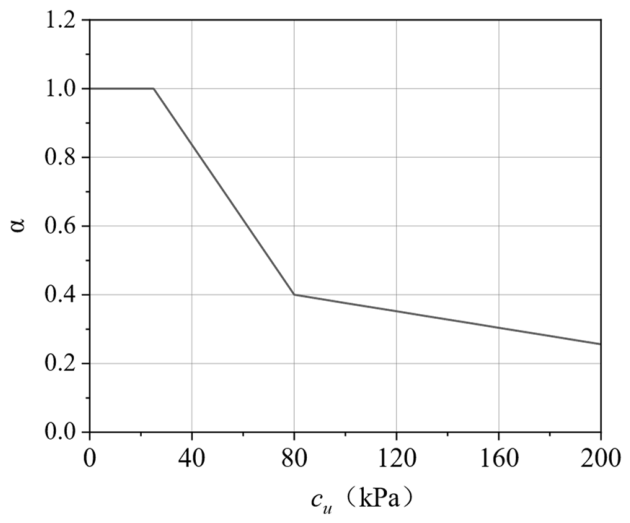
Based on the test results reported in [11], the lower-bound $\alpha$–$c_u$ relationship is shown in Figure 2. In the present study, the lower-bound curve was further fitted, and the fitted expression for $\alpha$ is given as follows:

$$\alpha =\left\{\begin{array}{c}1\\ -0.0109c_u+1.2725\\ -0.0012c_u+0.496\end{array}\begin{array}{c} \\ \\ \end{array}\begin{array}{c}{c}_u\le 25 \mathrm{k}\mathrm{P}\mathrm{a}\\ 25 \mathrm{k}\mathrm{P}\mathrm{a}<c_u\le 80 \mathrm{k}\mathrm{P}\mathrm{a}\\ 80 \mathrm{k}\mathrm{P}\mathrm{a}<c_u<200 \mathrm{k}\mathrm{P}\mathrm{a}\end{array}\right.$$

(10)

Experimental studies have shown that soil resistance generally increases with increasing loading frequency. A dynamic correction scheme was proposed based on the static p-y curve model by performing regression analysis on dynamic test results [24,25]. In the present study, the static p-y curve model for piles near slopes is modified using two alternative approaches—adjustment of the real stiffness component, and the spring and dashpot model—thereby establishing corresponding dynamic p-y curve models. The former provides a direct dynamic extension of the p-y relationship by modifying soil resistance, whereas the latter idealizes the dynamic soil reaction by an equivalent spring and dashpot system.

In this formulation, dynamic effects are introduced through equivalent frequency-dependent stiffness and damping, while the soil parameters used in the model, such as $E_s$ and $c_u$, are treated as representative values rather than evolving state variables. Accordingly, strain-dependent modulus degradation, cyclic degradation, and explicit soil plasticity accumulation are not considered in the present formulation.

In the real-component modification scheme, soil stiffness increases with the frequency of the applied load, and the dynamic p-y curve formulation is derived by directly modifying the static stiffness:

$$p_d\left(z\right)=p_{s\theta }\left(z\right)\left[1+\beta {a_0}^2+\kappa a_0{\left({\displaystyle \frac{\omega y}{d}}\right)}^{\varsigma }\right]$$

(11)

$$k_{py}={\displaystyle \frac{p_d\left(z\right)}{y}}$$

(12)

where $k_{py}$ denotes the stiffness of the dynamic p-y curve; $p_d\left(z\right)$ represents the dynamical modified soil reaction amplitude, and $a_0=\omega R/V_s$ denotes the dimensionless frequency. The constants $\beta$, $\kappa$ and $\varsigma$ are determined through curve fitting, and the corresponding determination method is summarized in

Table 1. Values for the constant parameters of the power-corrected clay p-y curve.

Soil Type	Description	$\mathit{\beta }$ $({\mathit{a}}_0\mathbf{<}0.025)$	$\mathit{\beta }$ $({\mathit{a}}_0\ge 0.025)$	$\mathit{\kappa }$	$\mathit{\varsigma }$
Soft clay	$c_u<50 \mathrm{k}\mathrm{P}\mathrm{a}$ $V_s<125 \mathrm{m}/\mathrm{s}$	−180	−200	80	0.18
Medium clay	$50<c_u<100 \mathrm{k}\mathrm{P}\mathrm{a}$ $125<V_s<175 \mathrm{m}/\mathrm{s}$	−120	−360	84	0.19
Stiff clay	$c_u>100 \mathrm{k}\mathrm{P}\mathrm{a}$ $V_s>175 \mathrm{m}/\mathrm{s}$	−2900	−828	100	0.19

[24,25].

In the imaginary-component modification scheme, the stiffness component is taken as the soil stiffness under static load conditions, whereas the frequency-dependent increase in soil resistance and the associated dynamic effects are primarily captured by the radiation-damping-related component. Previous experimental results indicate that, under constant-velocity conditions, the slopes of the dynamic and static p-y curves are nearly the same at a given displacement. Consequently, this model can reproduce the experimental observations. The expressions for stiffness and damping are given as follows:

$$k_d={\displaystyle \frac{p_{s\theta }\left(z\right)}{y}}$$

(13)

$$c_d={\displaystyle \frac{p_{s\theta }\left(z\right)\left[\beta {a_0}^2+\kappa a_0{\left(\frac{\omega y}{d}\right)}^{\varsigma }\right]}{2\omega y}}$$

(14)

where $k_d$ represents the dynamic stiffness, which is taken to be equal in magnitude to the static stiffness; $c_d$ denotes the damping coefficient and can be expressed in the form of an equivalent radiation damping:

$${\beta }_r={\displaystyle \frac{\omega c_d}{2k_d}}$$

(15)

where ${\beta }_r$ is associated with horizontally propagating waves generated at the pile–soil interface, while ${\beta }_s$ is related to the hysteretic energy dissipation within the soil medium; the system damping ${\beta }_{sys}$ and the complex stiffness $k_{py}$ can be expressed as [30,31]

$${\beta }_{sys}={\beta }_r+{\beta }_s$$

(16)

$$k_{py}=k_d\left(1+2i{\beta }_{sys}\right)$$

(17)

2.3. Dynamic Response Analysis of the Winkler Model

The pile–soil interaction model employs the BDWF approach, treating the pile as a linear, elastic Euler–Bernoulli beam. Soil reaction forces are calculated using nonlinear Winkler dynamic spring stiffness, expressed as $k_{py}y\left(z,t\right)$, where $y\left(z,t\right)$ represents the pile shaft displacement. This formulation yields the dynamic equilibrium equation of the pile in the horizontal direction:

$${\displaystyle \frac{\partial Q\left(z,t\right)}{\partial z}}+k_{py}y\left(z,t\right)+{\tilde{m}}_p{\displaystyle \frac{{\partial }^{2}y\left(z,t\right)}{\partial t^2}}=0$$

(18)

where $y\left(z,t\right)=y\left(z\right)e^{i\omega t}$; $Q(z,t)=E_p{I}_p{\displaystyle \frac{{\partial }^{3}y(z)}{\partial z^3}}{e}^{i\omega t}$; ${\tilde{m}}_p={\rho }_p{A}_p$; ${\displaystyle \frac{{\partial }^{2}y(z,t)}{\partial t^2}}=-{\omega }^{2}y(z)e^{i\omega t}$. Eliminating the time term $e^{i\omega t}$ simultaneously yields the differential.

$$E_p{I}_p{y}^{″″}\left(z\right)+\left(k_{py}-{\omega }^2{\tilde{m}}_p\right)y\left(z\right)=0$$

(19)

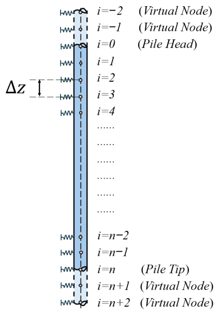
As pile–soil stiffness $k_{py}$ varies with pile displacement, analytical solutions are difficult to obtain. Therefore, the finite difference method is adopted to solve the fourth-order differential equation governing pile–soil interaction. As shown in Figure 3, the pile is divided into $n$ segment elements, each of length $∆z={\displaystyle \frac{L}{n}}$. The numbering of the segment elements starts from the pile top, with the top node numbered $0$ and the pile-tip node numbered $n$.

Two virtual nodes, $-1$ and $-2$, are added at the pile top, and two virtual nodes, $n+1$ and $n+2$, are added at the pile tip. In addition to the $n+1$ equations of the differential system, the inclusion of four boundary conditions at the pile top and tip allows pile displacements to be solved at all nodes. In the present study, the free head and free tip condition is adopted as the basic boundary condition. This idealization is commonly used to represent laterally loaded single piles with relatively weak rotational restraint at the pile head and without strong end fixity at the pile tip. Under this condition, both the pile head and pile tip are free in rotation and displacement. The shear force at the pile head represents the applied load, while the pile-head bending moment, pile-tip shear force, and pile-tip bending moment are set to zero. This yields the boundary conditions given in Equations (20)–(23):

$$E_p{I}_p{\displaystyle \frac{{\partial }^{2}y\left(z\right)}{\partial z^2}}{|}_{z=0}=0$$

(20)

$$E_p{I}_p{\displaystyle \frac{{\partial }^{3}y\left(z\right)}{\partial z^3}}{|}_{z=0}=H_0$$

(21)

$$E_p{I}_p{\displaystyle \frac{{\partial }^{2}y\left(z\right)}{\partial z^2}}{|}_{z=L}=0$$

(22)

$$E_p{I}_p{\displaystyle \frac{{\partial }^{3}y\left(z\right)}{\partial z^3}}{|}_{z=L}=0$$

(23)

The differential equations in Equations (20)–(23) can be transformed into difference equations by means of the central difference scheme, as follows:

$$y_1-2y_0+y_{-1}=0$$

(24)

$$E_p{I}_p{\displaystyle \frac{y_2-2y_1+2y_{-1}-y_{-2}}{2{∆z}^3}}=H_0$$

(25)

$$y_{n+1}-2y_n+y_{n-1}=0$$

(26)

$$y_{n+2}-2y_{n+1}+2y_{n-1}-y_{n-2}=0$$

(27)

Formulation of the matrix equations for single-pile responses is shown as

$${\left[K\right]}_{N\times N}{\left\{Y\right\}}_N={\left\{P\right\}}_N$$

(28)

Here, $N$ denotes the total number of nodes and can be determined from Equations (22)–(28):

$${\left[K\right]}_{N\times N}={\left[\begin{array}{ccccccccccc}0& 1& -2& 1& 0& \dots & 0& 0& 0& 0& 0\\ -1& 2& -2& 1& 0& \dots & 0& 0& 0& 0& 0\\ 1& -4& 6+{\delta }_0& -4& 1& \dots & 0& 0& 0& 0& 0\\ ⋮& ⋮& ⋮& ⋮& ⋮& \ddots & ⋮& ⋮& ⋮& ⋮& ⋮\\ 0& 0& 0& 0& 0& \dots & 1& -4& 6+{\delta }_n& -4& 1\\ 0& 0& 0& 0& 0& \dots & 0& 1& -2& 1& 0\\ 0& 0& 0& 0& 0& \dots & -1& 2& 0& -2& 1\end{array}\right]}_{N\times N}$$

(29)

$${\left\{P\right\}}_N=\left\{\begin{array}{c}0\\ 2{H_0∆z}^3\\ 0\\ 0\\ ⋮\\ 0\\ 0\\ 0\end{array}\right\}$$

(30)

$${\delta }_i={\displaystyle \frac{\left(k_{py}-{\omega }^2{\tilde{m}}_p\right){∆z}^4}{E_p{I}_p}}$$

(31)

The free head and free tip condition introduced above is adopted as the basic boundary condition in this study, and is also consistent with the assumption commonly used in previous studies on piles near slopes. The following verification and parametric analyses are mainly carried out for this basic condition. To facilitate further discussion of the influence of pile-head and pile-tip restraints, the corresponding boundary conditions and matrix formulations for additional constrained cases are also derived below.

A fixed head condition is considered to represent engineering cases in which the pile head is connected to a pile cap or superstructure and its rotation is therefore restrained. Under this condition, the pile-head rotation is set to zero, while the pile-head shear force still represents the applied horizontal load. The corresponding boundary conditions are given in Equations (32) and (33):

$$E_p{I}_p{\displaystyle \frac{\partial y\left(z\right)}{\partial z}}{|}_{z=0}=0$$

(32)

$$E_p{I}_p{\displaystyle \frac{{\partial }^{3}y\left(z\right)}{\partial z^3}}{|}_{z=0}=H_0$$

(33)

By using the central difference scheme, the corresponding difference equations and matrix equation under the fixed head condition can be obtained, as shown in Equations (34)–(36):

$$y_1-y_{-1}=0$$

(34)

$$E_p{I}_p{\displaystyle \frac{y_2-2y_1+2y_{-1}-y_{-2}}{2{∆z}^3}}=H_0$$

(35)

$${\left[K\right]}_{N\times N}={\left[\begin{array}{ccccccccccc}0& -1& 0& 1& 0& \dots & 0& 0& 0& 0& 0\\ -1& 2& -2& 1& 0& \dots & 0& 0& 0& 0& 0\\ 1& -4& 6+{\delta }_0& -4& 1& \dots & 0& 0& 0& 0& 0\\ ⋮& ⋮& ⋮& ⋮& ⋮& \ddots & ⋮& ⋮& ⋮& ⋮& ⋮\\ 0& 0& 0& 0& 0& \dots & 1& -4& 6+{\delta }_n& -4& 1\\ 0& 0& 0& 0& 0& \dots & 0& 1& -2& 1& 0\\ 0& 0& 0& 0& 0& \dots & -1& 2& 0& -2& 1\end{array}\right]}_{N\times N}$$

(36)

Furthermore, a fixed tip condition is considered to represent piles embedded in very stiff bearing strata or rock, for which both the displacement and rotation at the pile tip are restrained. The corresponding boundary conditions are expressed in Equations (37) and (38). By using the central difference scheme, the associated difference equations and matrix equation can be obtained as shown in Equations (39)–(41):

$$y\left(z\right){|}_{z=L}=0$$

(37)

$$E_p{I}_p{\displaystyle \frac{\partial y\left(z\right)}{\partial z}}{|}_{z=L}=0$$

(38)

$$y_n=0$$

(39)

$$y_{n+1}-y_{n-1}=0$$

(40)

$${\left[K\right]}_{N\times N}={\left[\begin{array}{ccccccccccc}0& -1& 0& 1& 0& \dots & 0& 0& 0& 0& 0\\ -1& 2& -2& 1& 0& \dots & 0& 0& 0& 0& 0\\ 1& -4& 6+{\delta }_0& -4& 1& \dots & 0& 0& 0& 0& 0\\ ⋮& ⋮& ⋮& ⋮& ⋮& \ddots & ⋮& ⋮& ⋮& ⋮& ⋮\\ 0& 0& 0& 0& 0& \dots & 1& -4& 6+{\delta }_n& -4& 1\\ 0& 0& 0& 0& 0& \dots & 0& 0& 1& 0& 0\\ 0& 0& 0& 0& 0& \dots & 0& 0& -1& 1& 0\end{array}\right]}_{N\times N}$$

(41)

The matrix equation in Equation (28) is solved to obtain the displacement response of the slope pile, from which the bending moments at each node are determined as

$${\left\{Y\right\}}_N={\left[K\right]}_{N\times N}^{-1}{\left\{P\right\}}_N$$

(42)

$$M_i=E_p{I}_p{\displaystyle \frac{{\partial }^2{y}_i\left(z\right)}{\partial z^2}}=E_p{I}_p{\displaystyle \frac{y_{i+1}-2y_i+y_{i-1}}{{∆z}^2}}$$

(43)

2.4. Iterative Computation Process

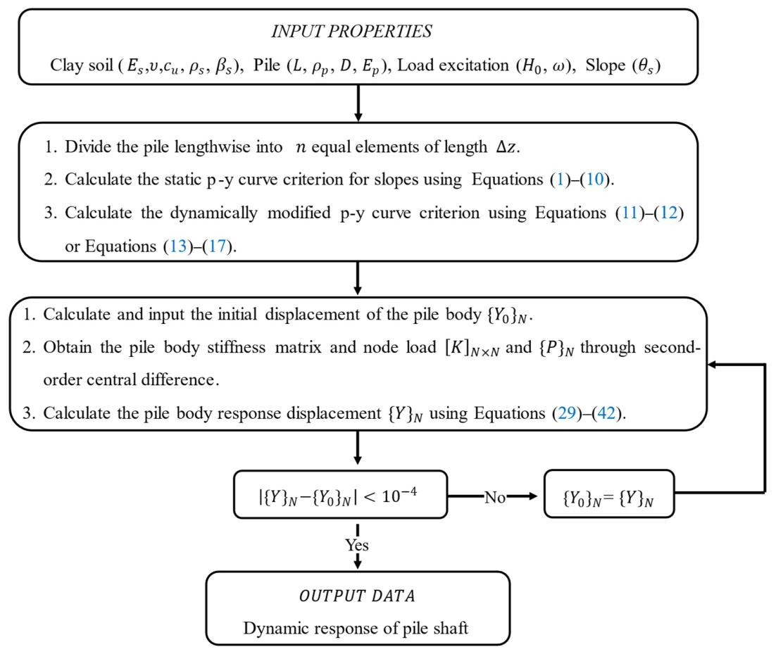
The proposed procedure for computing pile shaft displacement response dynamically updates the p-y spring parameters according to the relative displacement between the pile and the soil. Consequently, an iterative loop approach is adopted for the computation, and the specific calculation procedure is illustrated in Figure 4.

First, the pile is divided into n segments along its depth, and the initial lateral displacement ${\left\{Y_0\right\}}_N$ of the pile is calculated. The static p-y curve model is derived using Equations (1)–(10). Next, the dynamic-corrected p-y curve model is obtained based on Equations (11) and (12) and Equations (13)–(17). The pile stiffness matrix is then computed using the finite difference method. Subsequently, the horizontal displacement ${\left\{Y\right\}}_N$ of the pile is calculated according to Equations (29)–(42). The computed horizontal displacement ${\left\{Y\right\}}_N$ is used as the initial displacement ${\left\{Y_0\right\}}_N$ for the next iteration. The iterative process terminates when the difference between the calculated displacement ${\left\{Y\right\}}_N$ and the initial displacement ${\left\{Y_0\right\}}_N$ becomes sufficiently small $(|{\left\{Y\right\}}_N - {\left\{Y_0\right\}}_N < {10}^{-4})$. The final computed displacement ${\left\{Y\right\}}_N$ is then output as the displacement solution for the pile.

This study considers a steady-state, frequency-domain analysis. The resulting pile displacement ${\left\{Y\right\}}_N$ is a complex quantity. The real part represents the displacement component in phase with the input excitation, while the imaginary part corresponds to the displacement component associated with damping and is orthogonal to the in-phase component. Taking the modulus of the complex displacement at each node yields the displacement amplitude at that node.

$$|y_i| = \sqrt{\mathrm{Re}{(y_i)}^2 + \mathrm{Im}{(y_i)}^2}$$

(44)

3. Verification and Comparative Analysis

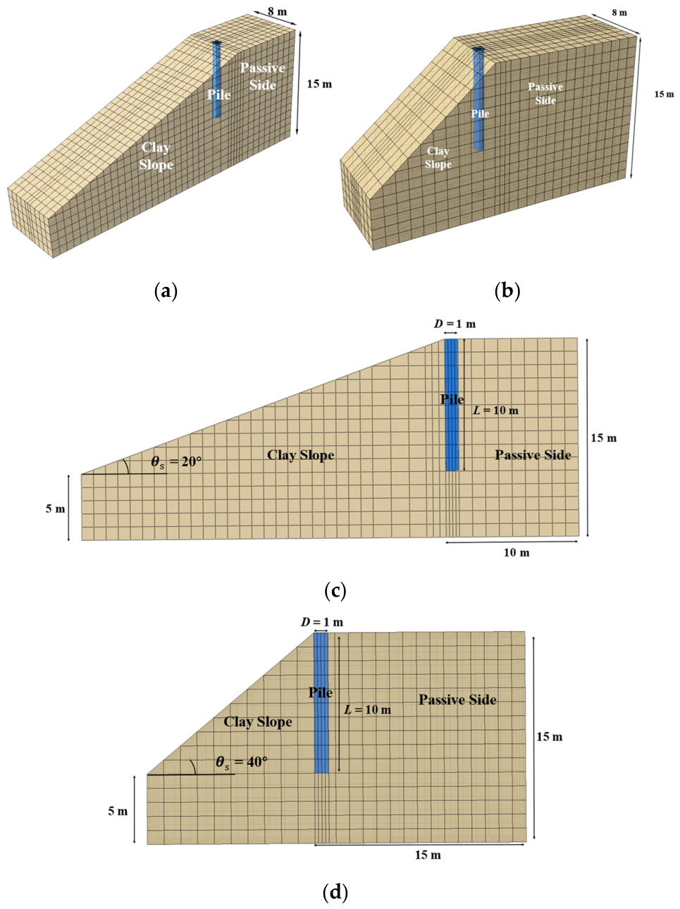
To assess the validity and accuracy of the theoretical solution for predicting the dynamic response of piles near slopes, the results obtained from the proposed modified p-y curve model were compared with those from finite element simulations performed using ABAQUS/Standard 2024. The finite element model and mesh are shown in Figure 5. The horizontal load excitation was applied uniformly to all nodes on the pile top in a cosine loading pattern. The geometric and material parameters of the slope–pile system were selected as detailed below [11]:

Soil: compressibility modulus E_s = 30.3 MPa; Poisson’s ratio v_s = 0.4; material damping β_s = 0.05; density ρ_s = (1800 kg)/m²; cohesion c_u = 70 kPa. Pile: diameter D = 1 m; elastic modulus E_p = 29 GPa; density ρ_p = 2500 kg/m². Slope angle: θ_s = 20° and 40°. Loading excitation: excitation frequency ω = 2 Hz and 5 Hz.

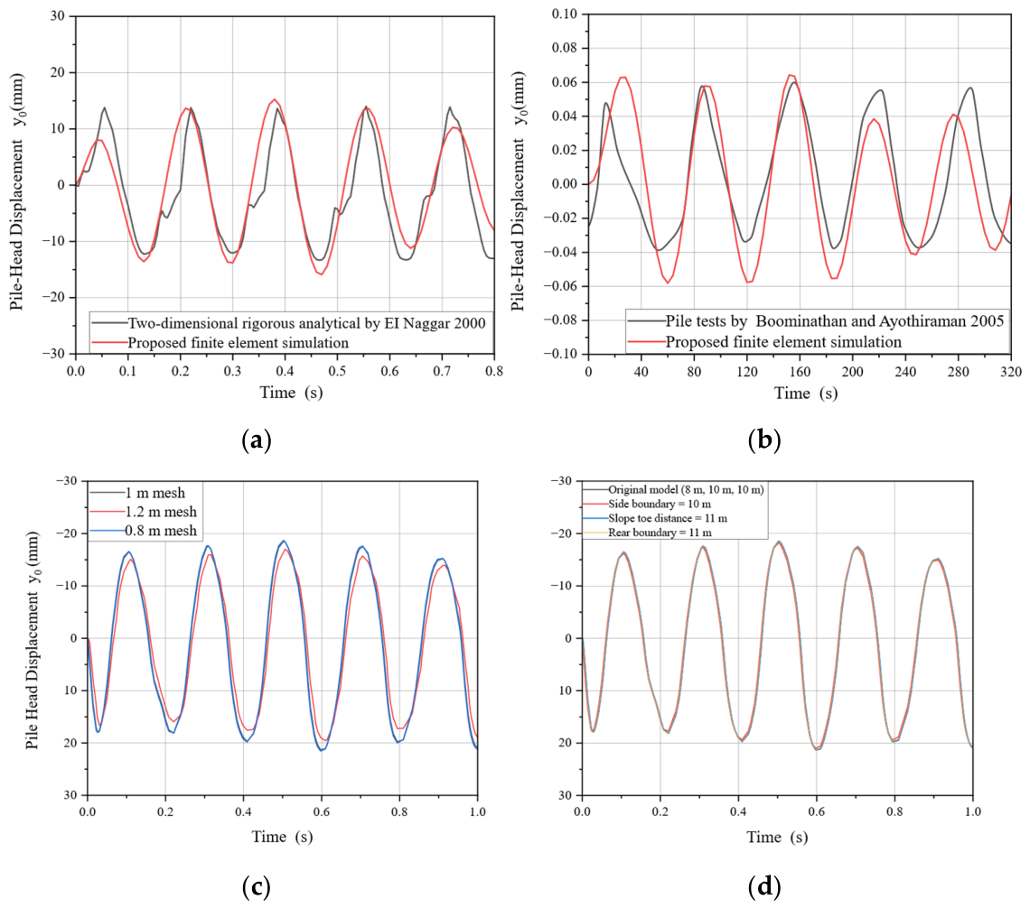
Figure 6 presents four aspects of finite element model verification. Figure 6a compares the pile-head displacement time history obtained from the present finite element model with the two-dimensional rigorous analytical solution of El Naggar [24] under a horizontal dynamic load of $100 \mathrm{kN}$ at $6 \mathrm{Hz}$. The two results show good agreement in overall waveform and oscillation period, indicating that the finite element model can reasonably reproduce the basic dynamic response of laterally loaded piles under flat-ground conditions. Figure 6b further compares the pile-head displacement time history obtained from the present finite element model with the pile test reported by Boominathan and Ayothiraman [32] under approximately similar conditions, with a pile diameter ratio of 10 and an excitation frequency of $14 \mathrm{Hz}$. The numerical and experimental results are generally consistent in the overall variation trend and periodic response pattern. Although some discrepancies remain in local peak values and phase due to differences in test conditions, material discreteness, and model idealization, the finite element model can still capture the main evolution of the pile-head displacement, indicating that it is suitable for simulating the lateral dynamic response of piles in clay. Figure 6c shows the mesh sensitivity analysis for the case of ${\theta }_s={20}^{\circ }$, $750 \mathrm{kN}$, and $5 \mathrm{Hz}$. The displacement amplitude obtained with the $1.2 \mathrm{m}$ mesh differs from that of the $1.0 \mathrm{m}$ mesh by about $9.5\%$, whereas the result from the $0.8 \mathrm{m}$ mesh differs from that of the $1.0 \mathrm{m}$ mesh by only about $0.9\%$. This indicates that the $1.0 \mathrm{m}$ mesh provides a reasonable balance between accuracy and computational efficiency. Figure 6d shows the boundary sensitivity analysis for the same loading case. After enlarging the side boundary, the slope-toe distance, and the rear boundary, only very small changes are observed in the pile-head response, with the amplitude deviations remaining within about $2\%$. Therefore, the selected model dimensions are sufficient to minimize boundary effects, and the finite element model is considered suitable as a numerical benchmark for the subsequent validation of the proposed theoretical method.

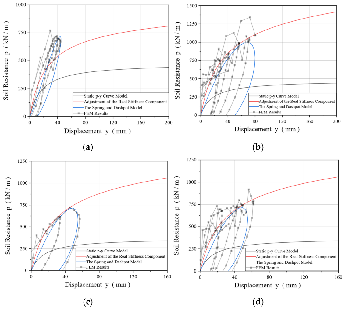
Figure 7 compares the p-y responses at a depth of $z=2 \mathrm{m}$ under four representative slope and frequency conditions. The FEM results show a clear hysteretic relation between soil reaction and pile displacement under cyclic loading. The real-component modification scheme gives a dynamic p-y curve without hysteresis and agrees well with the outer envelope of the FEM loops, showing that it can capture the backbone curve of the FEM p-y response well under slope conditions. By contrast, the spring and dashpot model yields a complex-valued soil reaction. Accordingly, the $p\left(t\right)$-$y\left(t\right)$ relation can be obtained from Equations (45) and (46). By contrast, the static p-y model cannot reflect the hysteretic feature or the variation in soil resistance under dynamic loading. The above results indicate that the correction parameters listed in Table 1 remain applicable to the slope conditions considered in this study.

$$y\left(t\right)=\mathrm{R}\mathrm{e}\left(y^{*}{e}^{i\omega t}\right)=\mathrm{R}\mathrm{e}\left(y^{*}\right)\mathrm{c}\mathrm{o}\mathrm{s}\omega t-\mathrm{I}\mathrm{m}\left(y^{*}\right)\mathrm{s}\mathrm{i}\mathrm{n}\omega t$$

(45)

$$\begin{array}{c}p\left(t\right)=Re\left(p^{*}{e}^{i\omega t}\right)=\mathrm{R}\mathrm{e}\left(p^{*}\right)\mathrm{c}\mathrm{o}\mathrm{s}\omega t-\mathrm{I}\mathrm{m}\left(p^{*}\right)\mathrm{s}\mathrm{i}\mathrm{n}\omega t\end{array}$$

(46)

where $y^{*}$ and $p^{*}$ denote the complex amplitudes of pile displacement and local soil reaction, respectively.

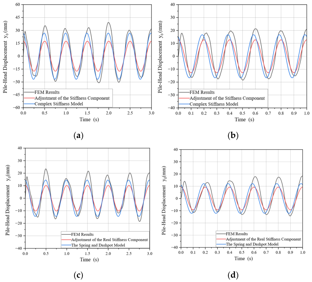
Figure 8 further compares the pile-head displacement time histories predicted by the two dynamic correction schemes with the FEM results under four representative loading cases. At the beginning of loading, the FEM response shows a certain transient lag relative to the theoretical solutions, which results in an evident phase difference in the early stage. After this transient effect gradually decays, the agreement between the theoretical and FEM responses becomes much closer. To quantify the prediction accuracy, the displacement amplitudes of the FEM and theoretical responses were evaluated for each case. The amplitude was determined, according to Equation (47), as the average half peak-to-trough value over several complete cycles, and the corresponding relative error was calculated using Equation (50). For each case, the amplitude was taken as the average half peak-to-trough value over several complete cycles. The relative amplitude errors of the adjustment of the real stiffness component are approximately $22.2\%$, $10.0\%$, $20.2\%$, and $15.3\%$ for the four cases in Figure 8, whereas those of the spring and dashpot model are reduced to about $6.1\%$, $3.6\%$, $10.5\%$, and $10.9\%$, respectively. These results show that both dynamic correction schemes can reproduce the overall oscillatory pattern of the pile-head response, while the spring and dashpot model provides consistently closer agreement with the FEM results and is therefore adopted in the subsequent analyses.

$$\begin{array}{c}{A}_{\mathrm{F}\mathrm{E}\mathrm{M}}={\displaystyle \frac{1}{m}}{\displaystyle \sum _{i=1}^m}{\displaystyle \frac{y_{max,i}-y_{min,i}}{2}}\end{array}$$

(47)

$$\begin{array}{c}\begin{array}{c}\epsilon ={\displaystyle \frac{|A_{\mathrm{t}\mathrm{h}}-A_{\mathrm{F}\mathrm{E}\mathrm{M}}|}{A_{\mathrm{F}\mathrm{E}\mathrm{M}}}}\times 100\%\end{array}\end{array}$$

(48)

where $A_{\mathrm{F}\mathrm{E}\mathrm{M}}$ and $A_{\mathrm{t}\mathrm{h}}$ denote the displacement amplitudes obtained from the FEM and theoretical method; $y_{max,i}$ and $y_{min,i}$ denote the maximum and minimum displacements within the $i-th$ cycle; and $\epsilon$ represents the relative error between the theoretical results and the finite element results.

This study compares various pile–soil interaction models to evaluate their suitability for analyzing the dynamic response of piles near slopes. In particular, the pile-head responses predicted by the proposed dynamic modified p-y curve model are compared with the finite element results, the static pile–soil interaction model for level ground, and the static p-y curve model for piles near slopes [11,15,31,33].

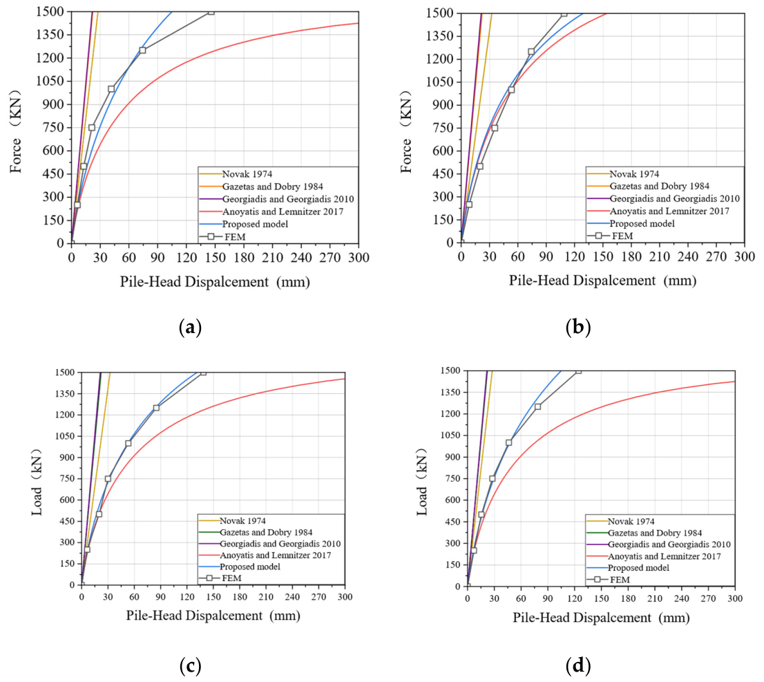
Figure 9 compares the pile-head load–displacement curves predicted by different design models under the same pile, soil, and loading conditions as those used in the preceding verification. It can be seen that the existing dynamic models developed for level-ground conditions generally predict a much stiffer pile–soil response than that obtained from the FEM analysis, and therefore underestimate the pile-head displacement under a given load. This is mainly because they do not account for the reduction in soil resistance caused by the slope effect. In contrast, the static p-y model for piles near slopes reflects the weakening of soil resistance, but tends to overestimate pile-head displacement, especially at larger load levels, because the changes in stiffness and damping under dynamic loading are not included. Compared with these existing methods, the proposed model gives the closest agreement with the FEM results over all four cases, and can better reproduce both the initial stiffness and the subsequent nonlinear development of the load–displacement response, indicating that the proposed dynamic extension can reasonably capture the combined influence of the slope effect and loading frequency on the overall pile-head response. Among the compared models, the proposed method shows the best overall performance in predicting the pile-head load–displacement response under slope conditions.

Therefore, the proposed model is mainly applicable to single piles near clay slopes subjected to steady dynamic lateral loading, where the overall response is governed primarily by local pile–soil interaction and moderate nonlinear behavior. Within the verification cases considered in this study, the spring and dashpot model gives pile-head displacement amplitude errors of about 3.6–10.9%, indicating that the simplified Winkler-based treatment can still provide reasonable engineering predictions for the global response. Nevertheless, the present model does not explicitly account for full three-dimensional continuum effects, soil layering, or more pronounced nonlinear soil deformation, and its applicability may be limited when these effects become dominant.

4. Parameter Analysis

This section provides a quantitative investigation of the horizontal dynamic response of slope piles in the context of nonlinear pile–soil interaction. The influence of various factors is examined, including pile diameter $D$, excitation frequency $\omega$, pile length $L$, friction coefficient $\alpha$, and slope angle ${\theta }_s$. The response quantities considered include the pile-head displacement amplitude, $\left|y_0\right|$, where $y_0$ is the complex displacement at the pile head; the maximum bending moment amplitude along the pile, $\mid M_{\mathrm{m}\mathrm{a}\mathrm{x}}\mid$; the pile-head stiffness $K_{hh}$; and the damping ratio ${\beta }_0$. The equivalent horizontal stiffness at the pile head ($K_{hh}$) is defined as the ratio of the horizontal load at the pile top ($H_0$) to the corresponding pile-head displacement ($\left|y_0\right|$), i.e., $K_{hh}=H_0/\left|y_0\right|$, and is used to characterize the overall lateral deformation resistance of the pile–soil system under horizontal dynamic loading, as well as the degree to which the supporting effect of the surrounding soil is mobilized. The complex stiffness at the pile head is correspondingly defined as $K_{hh}^{*}=H_0/y_0$. With reference to the correspondence between the complex stiffness loss factor and the damping ratio in a linear single-degree-of-freedom system, the equivalent damping ratio at the pile top is further defined as $\mathrm{I}\mathrm{m}(K_{hh}^{*})/[2\mathrm{R}\mathrm{e}(K_{hh}^{*})]$, which reflects energy dissipation of the pile–soil system at a given frequency.

The foundation parameters are as follows: soil modulus $E_s=30.3 \mathrm{M}\mathrm{P}\mathrm{a}$; shear modulus ${\upsilon }_s=0.4$; density ${\rho }_s=1800 \mathrm{k}\mathrm{g}/{\mathrm{m}}^2$; unconfined compressive strength $c_u=70 \mathrm{k}\mathrm{P}\mathrm{a}$. The elastic modulus of the pile is $E_p=29 \mathrm{G}\mathrm{P}\mathrm{a}$.

4.1. Pile Diameter

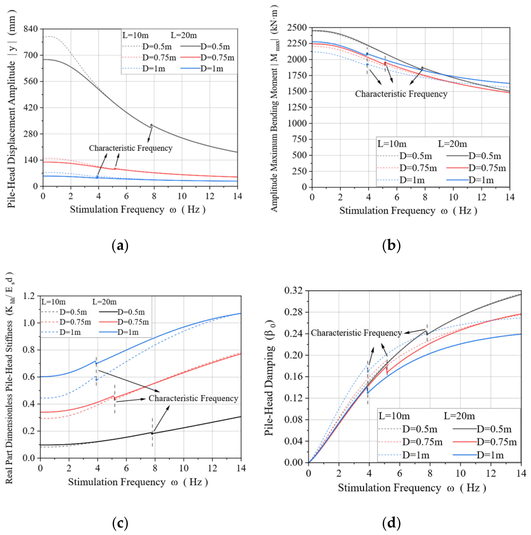
Figure 10 illustrates the effect of pile diameter on the lateral response of piles. It presents the pile-head responses for two pile lengths ($10 \mathrm{m}$ and $20 \mathrm{m}$) and three pile diameters ($D=0.5 \mathrm{m}$, $0.75 \mathrm{m}$ and $1 \mathrm{m}$) for piles near a slope with an angle of $40°$, when subjected to a horizontal load of $1000 \mathrm{k}\mathrm{N}$ at different excitation frequencies. As shown in Figure 10, minor abrupt changes can be observed in the vicinity of a certain frequency. Near this frequency, the pile-head stiffness and damping ratio change noticeably, whereas the pile-head displacement amplitude and the maximum bending moment vary only slightly. Therefore, this frequency should not be regarded as a conventional resonance frequency, but rather as a characteristic frequency associated with a change in the governing mechanism of pile–soil interaction.

For the spring and dashpot representation, the dynamic soil reaction may be written in the form $p=ky+c\dot{y}$. Under dynamic loading, the relative importance of the damping term to the stiffness term is controlled by $\mathsf{\omega }c/k$. Since the stiffness term scales with the soil shear modulus $G_s$, while the damping term scales with ${\mathsf{\rho }}_s{V}_{s}D$ and $G_s={\mathsf{\rho }}_s{V}_s^2$, one obtains $\mathsf{\omega }c/k\sim \mathsf{\omega }D/V_s$. This suggests that the characteristic frequency should scale with $V_s/D$, and may therefore be written in the form

$${\omega }_c=\mathrm{C}{\displaystyle \frac{V_s}{D}}$$

(49)

where $\mathrm{C}$ is a dimensionless constant. According to the transition points observed in Figure 8 for different pile diameters, the corresponding values of $\mathrm{C}$ are approximately concentrated around 0.05. Accordingly, the characteristic frequency in the present study may be expressed as follows:

$${\omega }_c\approx {\displaystyle \frac{V_s}{20D}}$$

(50)

The characteristic frequency has only a minor influence on the pile-head displacement amplitude and the maximum bending moment amplitude along the pile. For the smallest pile diameter of $D=0.5 \mathrm{m}$, the pile-head displacement amplitude increases by only $4.64\%$ near the characteristic frequency, whereas the effect is negligible for the other pile diameters. Meanwhile, the amplification effect on the maximum bending moment remains below $2\%$ for all pile diameters. Both pile-head stiffness and damping decrease at the characteristic frequency, with the amplification effect increasing as the pile diameter increases. Pile-head damping decreases by $7.87\%$ and $2.93\%$ for $D=1 \mathrm{m}$ and $D=0.5 \mathrm{m}$, respectively, while pile-head stiffness decreases by $3.86\%$ and $2.56\%$, respectively. Additionally, pile-head stiffness exhibits heightened sensitivity to excitation frequency at larger diameters. Compared to static conditions, pile-head stiffness increases by $214\%$ and $77.4\%$ at $D=1 \mathrm{m}$ and $D=0.5 \mathrm{m}$, respectively, under $14 \mathrm{H}\mathrm{z}$ excitation. Furthermore, frequency sensitivity increases with shorter pile lengths. However, pile-head displacement amplitude is more sensitive at smaller diameters, decreasing by $72.6\%$ and $49.1\%$ for $D=1 \mathrm{m}$ and $0.5 \mathrm{m}$, respectively. The influence of pile length also varies significantly across different diameters and frequencies. As the excitation frequency increases, the influence of pile length on pile-head stiffness, displacement amplitude, and maximum bending moment gradually diminishes. At sufficiently high excitation frequencies, pile length ceases to affect the results of the pile response.

4.2. Horizontal Load Amplitude

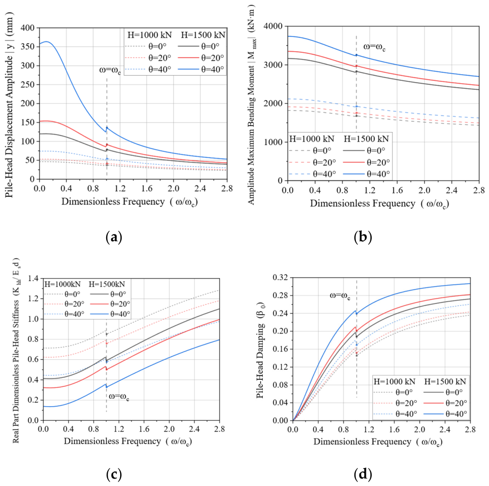
Figure 11 illustrates the variation in pile-head lateral response with excitation frequency for piles with a diameter of $1 \mathrm{m}$ and a length of $10 \mathrm{m}$, at different slope angles, and for two load conditions ($1000 \mathrm{k}\mathrm{N}$ and $1500 \mathrm{k}\mathrm{N}$). The excitation frequency was normalized based on the characteristic frequency, ${\omega }_c$. At the characteristic frequency, the displacement amplitude of the pile top on the slope with ${\theta }_s=40°$ increased by $8.97\%$ and $5.62\%$ under loads of $1500 \mathrm{k}\mathrm{N}$ and $1000 \mathrm{k}\mathrm{N}$, respectively. Similarly, the pile top stiffness decreased more significantly under the higher load. The sloping terrain also made the change in pile response around the characteristic frequency more pronounced. With an excitation of $1500 \mathrm{k}\mathrm{N}$, the displacement at the characteristic frequency for a pile top at an angle of $40°$ increased by $11.19 \mathrm{m}\mathrm{m}$. This exceeded the displacement for angles of $20°$ and $0°$ by $5.37 \mathrm{m}\mathrm{m}$ and $6.67 \mathrm{m}\mathrm{m}$, respectively. Furthermore, the characteristic frequency had a negligible impact on the maximum bending moment of the pile shaft. As can be seen in Figure 11, the influence of slope effect on pile-head displacement amplitude gradually diminishes as the excitation frequency increases. When the excitation frequency exceeds $2.4{\omega }_c$, pile-head displacements across different slopes become uniform. This suggests that high-frequency excitation suppresses the slope effect on pile-head displacement. In contrast, the slope effect on the maximum bending moment of the pile, pile top stiffness, and damping did not change significantly with frequency variation. Their influence remained largely consistent across different frequencies.

Additionally, compared to static conditions, piles on steep slopes exhibit greater sensitivity to excitation frequency. When the excitation load amplitude $H_0=1500 \mathrm{k}\mathrm{N}$, the displacement amplitude at the pile top under dynamic conditions ($\omega =2.8{\omega }_c$) decreased by $85.18\%$, $71.76\%$, and $67.05\%$ for slope angles of $40°$, $20°$, and $0°$, respectively, compared to static conditions. Simultaneously, pile-head stiffness increased by $4.7$, $2.1$, and $1.7$ times for these slope angles. The maximum bending moment of the pile decreased by approximately $26\%$ across all three slope angles, exhibiting identical frequency sensitivity. Furthermore, under sloping terrain conditions, larger excitation loads amplify the nonlinear characteristics of the pile–soil interaction, thereby enhancing the frequency sensitivity of pile shaft responses. For a slope angle of ${\theta }_s=40°$, the displacement amplitude and stiffness variation at the pile top increased by $26\%$ and $24\%$, respectively, for the $1500 \mathrm{k}\mathrm{N}$ load compared to the $1000 \mathrm{k}\mathrm{N}$ load.

4.3. Excitation Frequency

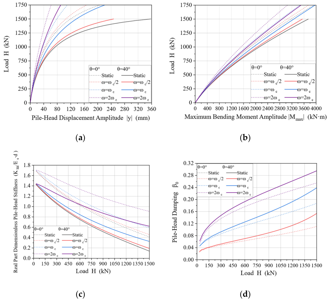
Figure 12 illustrates the load–parameter curves at different excitation frequencies. As expected, consistent with static conditions, an increase in lateral load amplitude leads to a reduction in pile-head stiffness, an increase in displacement amplitude, and higher maximum bending moments. The equivalent damping at the pile top shows a rapid-slowing–rapid increase trend as the load increases. It is also observed that the slope effect weakens with rising excitation frequency. At a load amplitude of $1500 \mathrm{k}\mathrm{N}$, the displacement amplitudes under $2{\omega }_c$ dynamic and ${\omega }_c$ dynamic excitation on sloping terrain are $138 \mathrm{m}\mathrm{m}$ and $69 \mathrm{m}\mathrm{m}$, respectively, representing increases of $74.5\%$ and $41.5\%$ compared to flat-ground conditions. Under the same load and excitation frequencies, pile-head stiffness decreases by $66.3\%$ and $31.7\%$, respectively. In contrast, the maximum bending moment of the pile demonstrates weaker frequency sensitivity, decreasing by $15.9\%$, $15.0\%$, and $14.6\%$ at $2{\omega }_c$, ${\omega }_c$, and $0.5{\omega }_c$, respectively. Additionally, the figures suggest that the slope effect on pile responses intensifies with increasing load.

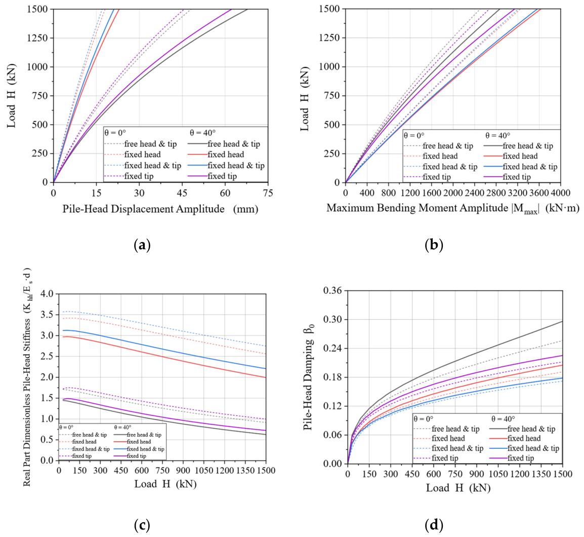
4.4. Pile-Head and Pile-Tip Constraints

In addition to the free head and free tip condition adopted in the preceding analyses, this section further examines the influence of pile-head and pile-tip constraints on the dynamic response of piles near slopes. Figure 13 compares the load–response curves under different pile-head and pile-tip constraints. The results show that the pile-head constraint plays a much more important role than the pile-tip constraint. At a load amplitude of $1500 \mathrm{k}\mathrm{N}$ and ${\theta }_s=40°$, the pile-head displacement amplitudes for the free head and tip, fixed head, fixed head and tip, and fixed tip cases are about $66 \mathrm{mm}$, $20 \mathrm{mm}$, $18 \mathrm{mm}$, and $58 \mathrm{mm}$, respectively, indicating that restraining pile-head rotation reduces the displacement amplitude by about $70\%$, whereas restraining the pile tip alone leads to only a limited reduction. A similar trend can also be observed in Figure 13b, where the maximum bending moment under the fixed head condition is about $24\%$ larger than that under the free head and tip condition, while the increase caused by tip restraint alone is relatively small. In addition, Figure 13c,d show that restraining the pile head significantly increases the equivalent horizontal stiffness, but reduces the damping ratio. For all four boundary conditions, the responses under ${\theta }_s=40°$ remain less favorable than those under flat ground, indicating that the slope effect and boundary constraint jointly influence the dynamic behavior of laterally loaded piles.

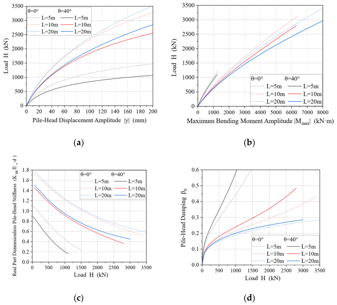
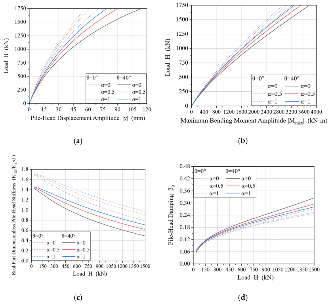
4.5. Pile Length and Interface Friction Coefficient

Figure 14 and Figure 15 examine the influence of pile length and adhesion coefficient on the response of the pile under $2{\omega }_c$ excitation for two terrain conditions: ${\theta }_s=0°$ and ${\theta }_s=40°$. Figure 14 shows that the overall trend of pile shaft response under loading aligns with the static state. Under identical loading conditions, the shorter pile ($L=5 \mathrm{m}$) exhibits lower pile-head stiffness, a smaller maximum bending moment, and greater pile displacement compared to the longer piles. The shorter pile demonstrates poorer performance in terms of pile-head displacement and stiffness, but better performance in terms of maximum bending moment and pile-head equivalent damping. Under $2{\omega }_c$ excitation, the dynamic responses of the $10 \mathrm{m}$ and $20 \mathrm{m}$ piles show little difference. Therefore, in practical engineering, a more economical pile length can be selected based on actual requirements. For the $5 \mathrm{m}$ short pile, when the load amplitude $H_0=1000 \mathrm{k}\mathrm{N}$, the pile top displacement on the slope increases by $116\%$ compared to flat-ground conditions, while pile top stiffness decreases by $53.6\%$. The amplification effect on maximum bending moment is not pronounced, and pile top damping shows slight amplification. For 20 m long piles, when the load amplitude $H_0=2800 \mathrm{k}\mathrm{N}$, the slope effect results in limited displacement amplification ($47.6\%$), limited damping amplification ($5.3\%$), and reduced stiffness ($31.96\%$). However, the slope significantly amplifies the maximum bending moment of long piles, increasing it by $21.4\%$ compared to flat-ground conditions.

5. Conclusions

This study extends the static p-y curve model for piles near slopes into a dynamic analysis framework by introducing frequency-dependent corrections to account for dynamic pile–soil interaction. By combining this model with the BDWF model, a theoretical calculation procedure is proposed for evaluating the dynamic response of piles near slopes while accounting for nonlinear pile–soil interaction. The accuracy and reliability of the proposed computational approach are validated through comparisons between the theoretical predictions and finite element method results. The main conclusions are summarized as follows:

1. The dynamic p-y curve model based on the spring and dashpot model agrees better with the finite element results than the model based on adjustment of the real stiffness component. For the four verification cases considered, the relative amplitude errors of the adjustment of the real stiffness component are about 10.0–22.2%, whereas those of the spring and dashpot model are reduced to about 3.6–10.9%.

2. The pile–soil system exhibits a characteristic frequency, which is mainly governed by the soil shear-wave velocity and pile diameter. The characteristic frequency may be expressed as ${\mathsf{\omega }}_c\approx V_s/\left(20D\right)$. Near this frequency, the pile-head displacement changes only slightly, whereas the pile-head stiffness and damping ratio decrease more noticeably. For $D=1 \mathrm{m}$, the corresponding reductions are about $3.86\%$ and $7.87\%$.

3. High-frequency excitation suppresses the influence of slope effect and pile length on pile-head displacement. As the excitation frequency increases, the displacement difference between slope and flat-ground conditions gradually decreases, and the responses of piles with different lengths tend to become closer. At sufficiently high excitation frequencies, the influence of pile length on pile-head displacement, pile-head stiffness, and maximum bending moment becomes very limited.

It should be noted that the present method is developed within an equivalent-linear dynamic framework for steady-state harmonic loading and follows the idealized slope geometry adopted in the underlying static slope p-y model. Therefore, more complex effects associated with soil nonlinearity, stratigraphic and geometric variability, full three-dimensional continuum interaction, and non-stationary broadband loading are not explicitly considered in the present formulation. These aspects deserve further investigation in future work.

References

1. Ren, S.; Tao, Z.; He, M.; Pang, S.; Li, M.; Xu, H. Stability Analysis of Open-Pit Gold Mine Slopes and Optimization of Mining Scheme in Inner Mongolia, China. J. Mt. Sci. 2020, 17, 2997–3011. [Google Scholar] [CrossRef] [Scilit]
2. Steiakakis, E.; Xiroudakis, G.; Lazos, I.; Vavadakis, D.; Bazdanis, G. Stability Analysis of a Multi-Layered Slope in an Open Pit Mine. Geosciences 2023, 13, 359. [Google Scholar] [CrossRef] [Scilit]
3. Zhang, J.; Liu, X.; Jia, H.; Du, X.; Wang, Z.; Pan, G.; Zhang, M. Fitting of Anisotropic Strength Parameters of Laminated Shale and Its Influence on Wellbore Instability. Geomech. Geophys. Geo-Energy Geo-Resour. 2025, 11, 43. [Google Scholar] [CrossRef] [Scilit]
4. Huang, Y.; Wang, P.; Zhao, M.; Zhang, C.; Du, X. Dynamic Responses of an End-Bearing Pile Subjected to Horizontal Earthquakes Considering Water-Pile-Soil Interactions. Ocean. Eng. 2021, 238, 109726. [Google Scholar] [CrossRef] [Scilit]
5. Lin, C.; Liu, Q.; Deng, T.; Liu, T. Kinematic Response of Floating Piles in Two-Layered Soils Subjected to Vertically Incident S-Waves. Comput. Geotech. 2024, 166, 106006. [Google Scholar] [CrossRef] [Scilit]
6. Liu, P.; Jiang, C.; Lin, M.; Chen, L.; He, J. Nonlinear Analysis of Laterally Loaded Rigid Piles at the Crest of Clay Slopes. Comput. Geotech. 2020, 126, 103715. [Google Scholar] [CrossRef] [Scilit]
7. Liu, P.; Chen, L.; Huawei, C.; Jiang, C. A Method for Predicting Lateral Deflection of Large-Diameter Monopile near Clay Slope Based on Soil-Pile Interaction. Comput. Geotech. 2021, 135, 104180. [Google Scholar] [CrossRef] [Scilit]
8. Jiang, C.; Lin, M.; Liu, P. Study on Calculation Method of Lateral Characteristics of Offshore Pile near Layered Soil Slope. Ocean. Eng. 2023, 289, 116245. [Google Scholar] [CrossRef] [Scilit]
9. Liu, P.; Jiang, C. A New p-y Curve Criterion for Piles in Proximity to Undrained Clay Slopes. Comput. Geotech. 2023, 164, 105801. [Google Scholar] [CrossRef] [Scilit]
10. Wu, J.; Pu, L.; Zhai, C. A Review of Static and Dynamic P-y Curve Models for Pile Foundations. Buildings 2024, 14, 1507. [Google Scholar] [CrossRef] [Scilit]
11. Georgiadis, K.; Georgiadis, M. Undrained Lateral Pile Response in Sloping Ground. J. Geotech. Geoenviron. Eng. 2010, 136, 1489–1500. [Google Scholar] [CrossRef] [Scilit]
12. Georgiadis, K.; Georgiadis, M. Development of p–y Curves for Undrained Response of Piles near Slopes. Comput. Geotech. 2012, 40, 53–61. [Google Scholar] [CrossRef] [Scilit]
13. Nimityongskul, N.; Kawamata, Y.; Rayamajhi, D.; Ashford, S.A. Full-Scale Tests on Effects of Slope on Lateral Capacity of Piles Installed in Cohesive Soils. J. Geotech. Geoenviron. Eng. 2018, 144, 04017103. [Google Scholar] [CrossRef] [Scilit]
14. Qian, Z.-Z.; Lu, X.-L.; Yang, W.-Z. Comparative Field Tests on Straight-Sided and Belled Piers on Sloping Ground under Combined Uplift and Lateral Loads. J. Geotech. Geoenviron. Eng. 2019, 145, 04018099. [Google Scholar] [CrossRef] [Scilit]
15. Novak, M. Dynamic Stiffness and Damping of Piles. Int. J. Rock Mech. Min. Sci. Geomech. Abstr. 1974, 12, 64. [Google Scholar] [CrossRef] [Scilit]
16. Novak, M.; Nogami, T. Soil-pile Interaction in Horizontal Vibration. Earthq. Eng. Struct. Dyn. 1977, 5, 263–281. [Google Scholar] [CrossRef] [Scilit]
17. Mylonakis, G. Elastodynamic Model for Large-Diameter End-Bearing Shafts. Soils Found. 2001, 41, 31–44. [Google Scholar] [CrossRef] [Scilit] [PubMed]
18. Nogami, T.; Novak, M. Resistance of Soil to a Horizontally Vibrating Pile. Earthq. Eng. Struct. Dyn. 1977, 5, 249–261. [Google Scholar] [CrossRef] [Scilit]
19. Anoyatis, G.; Mylonakis, G.; Lemnitzer, A. Soil Reaction to Lateral Harmonic Pile Motion. Soil Dyn. Earthq. Eng. 2016, 87, 164–179. [Google Scholar] [CrossRef] [Scilit]
20. Lin, C.; Liu, Q.; Deng, T.; Zeng, L. Kinematic Response of the Single Floating Piles in the Two-Layered Soil Subjected to Vertically Incident P-Waves. Ocean. Eng. 2024, 291, 116517. [Google Scholar] [CrossRef] [Scilit]
21. Lee, V.W.; Sherif, R.I. Diffraction around Circular Canyon in Elastic Wedge Space by Plane SH-Waves. J. Eng. Mech. 1996, 122, 539–544. [Google Scholar] [CrossRef] [Scilit]
22. Liu, Q.; Wu, Z.; Lee, V.W. Scattering and Reflection of SH Waves around a Slope on an Elastic Wedged Space. Earthq. Eng. Eng. Vib. 2019, 18, 255–266. [Google Scholar] [CrossRef] [Scilit]
23. Ke, W. Kinematic Response of a Pile within a Soil Slope to SH Wave Excitation. Soil Dyn. Earthq. Eng. 2024, 183, 108730. [Google Scholar] [CrossRef] [Scilit]
24. El Naggar, M.H.; Bentley, K.J. Dynamic Analysis for Laterally Loaded Piles and Dynamic P-y Curves. Can. Geotech. J. 2000, 37, 1166–1183. [Google Scholar] [CrossRef]
25. Mostafa, Y.E.; Naggar, M.H.E. Dynamic Analysis of Laterally Loaded Pile Groups in Sand and Clay. Can. Geotech. J. 2002, 39, 1358–1383. [Google Scholar] [CrossRef] [Scilit]
26. Murchison, J.M.; O’Neill, M.W. Evaluation of P-y Relationships in Cohesionless Soils. Int. J. Rock Mech. Min. Sci. Geomech. Abstr. 1986, 23, 109. [Google Scholar] [CrossRef] [Scilit]
27. Tak Kim, B.; Kim, N.-K.; Jin Lee, W.; Su Kim, Y. Experimental Load–Transfer Curves of Laterally Loaded Piles in Nak-Dong River Sand. J. Geotech. Geoenviron. Eng. 2004, 130, 416–425. [Google Scholar] [CrossRef] [Scilit]
28. Liang, R.; Yang, K.; Nusairat, J. P-y Criterion for Rock Mass. J. Geotech. Geoenviron. Eng. 2009, 135, 26–36. [Google Scholar] [CrossRef] [Scilit]
29. Rajashree, S.S.; Sitharam, T.G. Nonlinear Finite-Element Modeling of Batter Piles under Lateral Load. J. Geotech. Geoenviron. Eng. 2001, 127, 604–612. [Google Scholar] [CrossRef] [Scilit]
30. Anoyatis, G.; Di Laora, R.; Mandolini, A.; Mylonakis, G. Kinematic Response of Single Piles for Different Boundary Conditions: Analytical Solutions and Normalization Schemes. Soil Dyn. Earthq. Eng. 2013, 44, 183–195. [Google Scholar] [CrossRef] [Scilit]
31. Anoyatis, G.; Lemnitzer, A. Kinematic Winkler Modulus for Laterally-Loaded Piles. Soils Found. 2017, 57, 453–471. [Google Scholar] [CrossRef] [Scilit]
32. Boominathan, A.; Ayothiraman, R. Dynamic Behaviour of Laterally Loaded Model Piles in Clay. Proc. Inst. Civ. Eng.-Geotech. Eng. 2005, 158, 207–215. [Google Scholar] [CrossRef] [Scilit]
33. Gazetas, G.; Dobry, R. Horizontal Response of Piles in Layered Soils. J. Geotech. Eng. 1984, 110, 20–40. [Google Scholar] [CrossRef] [Scilit]
Figure 1. Schematic diagram of the model.
Applsci 16 04780 g001
Figure 2. Adhesion factor versus c u relationships for piles and drilled shafts.
Applsci 16 04780 g002
Figure 3. Winkler foundation beam under the finite difference method.
Applsci 16 04780 g003
Figure 4. Flowchart of the computational program for dynamic response analysis of piles near slopes.
Applsci 16 04780 g004
Figure 5. Finite element model and mesh generation: (a) θ s = 20 ° three-dimensional model; (b) θ s = 20 ° three-dimensional model; (c) θ s = 40 ° cross section (d) θ s = 20 ° cross section.
Applsci 16 04780 g005
Figure 6. Finite element model verification: (a) comparison with the two-dimensional rigorous analytical solution ( 100   k N , 6   H z ) [24]; (b) comparison of pile foundation test results ( L / D = 10 , 14   H z ) [32]; (c) mesh sensitivity analysis ( θ s = 20 ° , 750   k N , 5   H z excitation); (d) boundary sensitivity analysis ( θ s = 20 ° , 750   k N , 5   H z excitation).
Applsci 16 04780 g006
Figure 7. Comparison of p-y curve results at buried depth of 2 m: (a) θ s = 20 ° , 2   H z ; (b) θ s = 20 ° , 5   H z ; (c) θ s = 40 ° , 2   H z ; (d) θ s = 40 ° , 5   H z .
Applsci 16 04780 g007
Figure 8. Displacement time-history curves at the pile top for two p-y curve models and a finite element model: (a) θ s = 20 ° , 750   k N , 2   H z excitation; (b) θ s = 20 ° , 750   k N , 5   H z excitation; (c) θ s = 40 ° , 500   k N , 2   H z excitation; (d) θ s = 40 ° , 500   k N , 5   H z excitation.
Applsci 16 04780 g008
Figure 9. Pile-head load–displacement curves under different design models: (a) ω = 2   H z , θ s = 20 ° ; (b) ω = 5   H z , θ s = 20 ° ; (c) ω = 2   H z , θ s = 40 ° ; (d) ω = 5   H z , θ s = 40 ° [11,15,31,33].
Applsci 16 04780 g009
Figure 10. Dynamic response characteristics of pile near sloping terrain under different pile diameter conditions ( H 0 = 1000   k N , θ s = 40 ° ): (a) pile-head displacement amplitude; (b) maximum bending moment amplitude; (c) equivalent horizontal stiffness at the pile head; (d) equivalent damping ratio at the pile head.
Applsci 16 04780 g010
Figure 11. Dynamic response characteristics of piles near sloping terrain under different load conditions ( D = 1   m , L = 10   m ): (a) pile-head displacement amplitude; (b) maximum bending moment amplitude; (c) equivalent horizontal stiffness at the pile head; (d) equivalent damping ratio at the pile head.
Applsci 16 04780 g011
Figure 12. Frequency-dependent response curves for piles ( D = 1   m , L = 10   m ): (a) pile-head displacement amplitude; (b) maximum bending moment amplitude; (c) equivalent horizontal stiffness at the pile head; (d) equivalent damping ratio at the pile head.
Applsci 16 04780 g012
Figure 13. Dynamic response under different pile-head and pile-tip constraints ( D = 1   m , L = 10   m , 5   Hz ): (a) pile-head displacement amplitude; (b) maximum bending moment amplitude; (c) equivalent horizontal stiffness at the pile head; (d) equivalent damping ratio at the pile head.
Applsci 16 04780 g013
Figure 14. Load−response curves for different pile lengths under 2 ω c excitation ( D = 1   m ): (a) pile-head displacement amplitude; (b) maximum bending moment amplitude; (c) equivalent horizontal stiffness at the pile head; (d) equivalent damping ratio at the pile head.
Applsci 16 04780 g014
Figure 15. Load−response curves for different adhesion coefficients at a frequency of 2 ω c ( D = 1   m , L = 10   m ): (a) pile-head displacement amplitude; (b) maximum bending moment amplitude; (c) equivalent horizontal stiffness at the pile head; (d) equivalent damping ratio at the pile head.
Applsci 16 04780 g015