An Expert Study on the Significance of Passenger Transport Characteristics in Choosing a Mode of Travel, Using Multi-Criteria Decision-Making Methods

Abstract

Passengers choose a mode of public transport from the available options based on characteristics that are important to them. The importance of these characteristics has received little research attention and varies. This study presents 10 characteristics of passenger transport, the significance of which was examined using four MCDM (multi-criteria decision-making) methods. The questionnaire was conducted and 27 specialists (experts) in road, rail and air transport rated the importance of various characteristics (criteria) using rankings, percentage weights and intensity of importance values derived from pairwise criterion comparisons using the Analytic Hierarchy Process (AHP). The results of the study show that the opinions of the expert panel, expressed as ratings, were consistent, as the Kendall’s coefficient of concordance (0.64) was 9.2 times greater than its minimum threshold value of 0.07. The ranks of the criteria were used to calculate their relative weights using the ARTIW-L (average rank transformation into weight–linear) and ARTIW-N (non-linear) methods. The relative weights were calculated from the criteria percentage weights using the DPW (direct percentage weight) method. The consistency ratios of all 27 matrices calculated using the AHP method were less than 0.1. This demonstrates their consistency. The average calculated for each criterion using the four MCDM methods is the final measure of the significance of the passenger transport characteristic. For experts, the most important factors were safety (0.2234), travel costs (0.1488), travel time (0.1465), and comfort (0.1181). Factors of moderate importance included door-to-door delivery (0.0847), environmental friendliness (0.0685), and vehicle capacity (0.0597). The following factors were deemed the least important: service quality (0.0571), the impact of weather conditions (0.0532) and the risk of contracting COVID-19 (0.0400). The most important criterion was 5.6 times more significant than the least important criterion. This data will be used to carry out a thorough evaluation of the different transport options and select the most suitable one for intercity passenger transport.

1. Introduction

People move to new places for various reasons, such as to live, go on holiday or fulfil their obligations [1]. The mode of travel selected depends on the traveller’s characteristics, such as age, gender or impairment. The choice may also be influenced by household characteristics: income, place of residence, and access to transportation. The choice of travel mode is often influenced by the purpose of the journey, the traveller’s perspective and personal values. When choosing a mode of public transport, (PT modes) passengers primarily consider the vehicle itself, how easy it is to board and alight from it (access/egress), and waiting times [2]. Income, ticket prices, and travel distance continue to be the main factors influencing passengers’ choices [3]. In developing countries, social factors have the greatest influence on travel behavior [4]. Given that rail transport competes with air and road transport, a system of criteria has been developed to determine why rail passengers choose this mode of transport as an alternative to other modes of transport [5].

Recently, people’s attitudes towards travel have changed. There are few studies that analyze the relationship between the choice of travel mode and travel satisfaction [6]. Studies show that people’s attitudes towards travel influence their choice of travel mode. There have been few studies examining whether people choose the right mode of transport. An analysis of leisure travel among 1656 respondents in the city of Ghent (Belgium) showed that approximately half of the respondents choose an inappropriate mode of transportation [7]. Travel planning involving autonomous vehicles is increasingly attracting the attention of researchers and professionals who are addressing issues related to their integration into the overall urban transportation system [8]. Travelling by car is not necessarily the best option. There are cheaper transportation alternatives that are safer for human health and the environment. The analysis of automobile commuters’ mode choice behaviour under the influence of simulated multimodal traveller information was conducted by developing two logit models [9]. The studies aim to gain a better understanding of the factors influencing the choice of transport mode among travelers in Penang, Malaysia [10]. The results of a study conducted in China show that most residents, apart from those who own a car and/or have a driver’s license, tend to choose slower modes of transportation (including walking and cycling) [11]. A new approach to spatial modelling of mode choice has been developed [12].

Inefficient public transportation is considered a common problem in any city or country. The reasons why daily commuters choose a particular mode of transportation are identified. The quality of public transport offered to users has been examined, as has its influence on their choice of transport mode [13]. Most people usually commute to and from work in the same way. Reimbursement by the employer for using a certain mode is the most important determinant influencing the experienced choice set, followed by ownership characteristics and urban density [14]. With the city’s population growing rapidly, it is essential to implement sustainable and efficient transportation systems. By doing so, the aim is to promote economic growth and social inclusion, and to increase mobility and accessibility. There is a study that examines the commuting choices of residents of Lusaka, Zambia, when traveling to work or school, as well as the factors influencing these choices. It has been found that public buses are the most common mode of transportation. Next come walking and travel by private car. Travel behaviour was also influenced by the density of residential buildings. In densely populated areas, priority was given to public transportation and walking. In sparsely populated areas, people tended to travel more by private vehicle. The main factors influencing the choice of transportation were travel time, cost, and safety. Environmental concerns had less significant impact on the choice of travel mode. The choice of transportation mode was significantly influenced by socioeconomic and demographic characteristics, such as age, gender, income, education, employment status, car ownership, purpose of the trip, household composition, children, and accessibility of the destination [15].

Taking the bus can be an attractive alternative to driving a private car. Although railways involve significant upfront costs when compared to other forms of public transport, they are a sound long-term investment. Trains can carry more passengers than buses. Trains cause less air pollution. Intercity passenger rail is a particularly popular mode of transport in Europe and an excellent alternative to private cars. In comparison to driving, travelling by train can be much more efficient in terms of miles per passenger [16]. Despite widespread claims about the benefits of ride-hailing (RH) services, few studies have been conducted in this area. A study was conducted to assess the willingness of transport users in Munich to use RH services [17]. The results of a study conducted in southwest England show that understanding the dynamics of travel behaviour encourages people to avoid high-carbon transportation [18]. The “utility” of a mode of transport is analyzed by evaluating two main groups of factors that influence the market: the price and quality of services (travel time, frequency, comfort, etc.) [19]. When modelling the choice between a regional train, a regional bus, and a car, the HII-I (Hierarchical Information Integration) method is applied [20].

Air pollution is a threat to public health. Carbon dioxide emissions are contributing to global warming. Many studies on public transport have shown that potential passengers consider rail to be superior to buses [21]. However, the construction of railway infrastructure and roads also has a negative environmental impact [22,23]. It is not always clear which option is the most eco-friendly: traveling by plane, train, or car. A comparative assessment of travelling by train and by plane has also been conducted [24]. Although the environmental impact of aviation emissions is much greater than that of rail transport when calculated on a passenger-kilometre basis, flying is not necessarily the most environmentally harmful option. The imbalance among these modes of transport highlights the need for other alternative modes of travel.

To improve passenger transport services, it is crucial to increase competitiveness. Long-distance passenger transport is usually carried out by air and rail. Travel time and cost, as well as the quality and variety of services and other economic criteria, have a significant influence on the choice of one of the competing modes of transport [25]. To analyze the choice between air travel and high-speed rail, a study was conducted on the Jakarta–Surabaya route [26]. Railways have an apparent advantage over other modes of transport for middle- and long-distance travel. The optimal distance for high-speed rail is 500–1000 km, for express trains it is 1000–2200 km, and for air travel it is over 2200 km. Correlations between vehicle emissions and air quality have also been examined [27]. Alternative transportation can benefit people’s health and economic activity.

A major challenge facing today’s transportation system is the increasing traffic congestion in cities. Many researchers recognise the significance of sustainable travel from a social, environmental and economic standpoint. There is a growing number of studies analyzing travel behavior. When a traveller decides to travel, the choice of travel route and mode of travel are interrelated [28]. The concept of “substitutability” is proposed and defined as the replacement of one mode of travel with a less desirable alternative [29]. This is particularly relevant when there are no viable alternatives, e.g., due to labor strikes, weather conditions, power outages, etc. Substitutability is a promising new concept that is relevant to research on travel behavior (Travel alternatives in this context can include activities, modes of transport, time of day, and routes). There are massive traffic jams in Beijing. Smartphones and route recommendation systems make it easier to choose a mode of transportation. It has been observed that, when planning a journey, passengers tend to choose the option suggested by the route recommendation system first and foremost. In the future, transport policymakers should take this into account to encourage passengers to choose more environmentally sustainable and eco-friendly modes of transport [30]. A study was conducted to analyse the factors influencing mode choice and to determine the level of passenger satisfaction with public transport services in terms of safety, comfort, convenience, flexibility and affordability. It shows that flexibility is the most significant factor influencing passenger satisfaction. This is followed by safety, convenience, and comfort, as well as cost [31]. Recent advancements in intelligent transportation systems are presented, focusing on complex mobility and network optimization [32,33].

In recent years, the most popular MCDM methods in the transport sector are the following [34]: TOPSIS method (used to assess the sustainable development of road transport, environmental effects of transport, and to prioritize transportation projects); AHP method (used to evaluate public road transportation vehicles and optimum rail route/station locations, and to analyze the severity of road accidents); Fuzzy AHP method (used to assess passenger satisfaction and assess infrastructure alternatives); CRITIC method (used to assess road safety, evaluate railway transportation performance, and analyze the spatiotemporal variation in transit accessibility). These methods have advantages [35] and disadvantages [36]. Alternative MCDM methods applied to the same problem often produce divergent results; therefore, to enhance reliability, an integrated system of MCDM methods is proposed. When searching for a more reliable tool, a system of MCDM methods is proposed to solve a single problem [37]. Passengers choose a mode of public transport from the available options based on characteristics that are important to them. The importance of these characteristics has received little research attention. This article presents an expert investigation of the importance of passenger transport properties for choice of trip mode using four MCDM methods: AHP, ATIW-L, ARTIW-N, and DPW. A comparative analysis of the relative weights of criteria calculated using these methods was conducted.

The goal of the study is to develop a framework that identifies the factors influencing the quality of public transport and travel mode choice. Then, determine the relative importance of these factors based on quantitative expert assessments using multi-criteria decision-making methods. Finally, conduct a comprehensive analysis of this importance.

This study consists of an introduction that provides an analysis of scientific works on the characteristics of passenger transport, with the research objective formulated at the end. Four MCDM methods applied in the study are presented. Using these methods, statistical indicators of the percentage weights of the 10 criteria ranks obtained from the expert survey and the AHP method were calculated and analyzed, leading to the formulation of the research conclusions.

2. Materials and Methods

2.1. A Model for Assessing the Significance of Criteria

Passengers value the features of public transportation that affect the quality of their journey. The quality of a journey is a multifaceted and complex concept that reflects how well it meets the passenger’s expectations and requirements. Passengers who have the option of travelling from their point of departure to their point of arrival using several modes of transport will choose the option that best suits their needs. The choice of alternatives is influenced by the significance of transport characteristics, which is examined in this study.

By understanding the views of passengers and transport experts on the most influential criteria, decision-makers responsible for the management and development of passenger transport companies can plan operations in a way that maximises economic, environmental and social benefits.

As the indicators describing the subject of the study do not all have the same impact on the objective at hand, determining the significance of these indicators is a very important task. The most used approach is subjective assessment, in which the weights of the indicators are determined by experts [38].

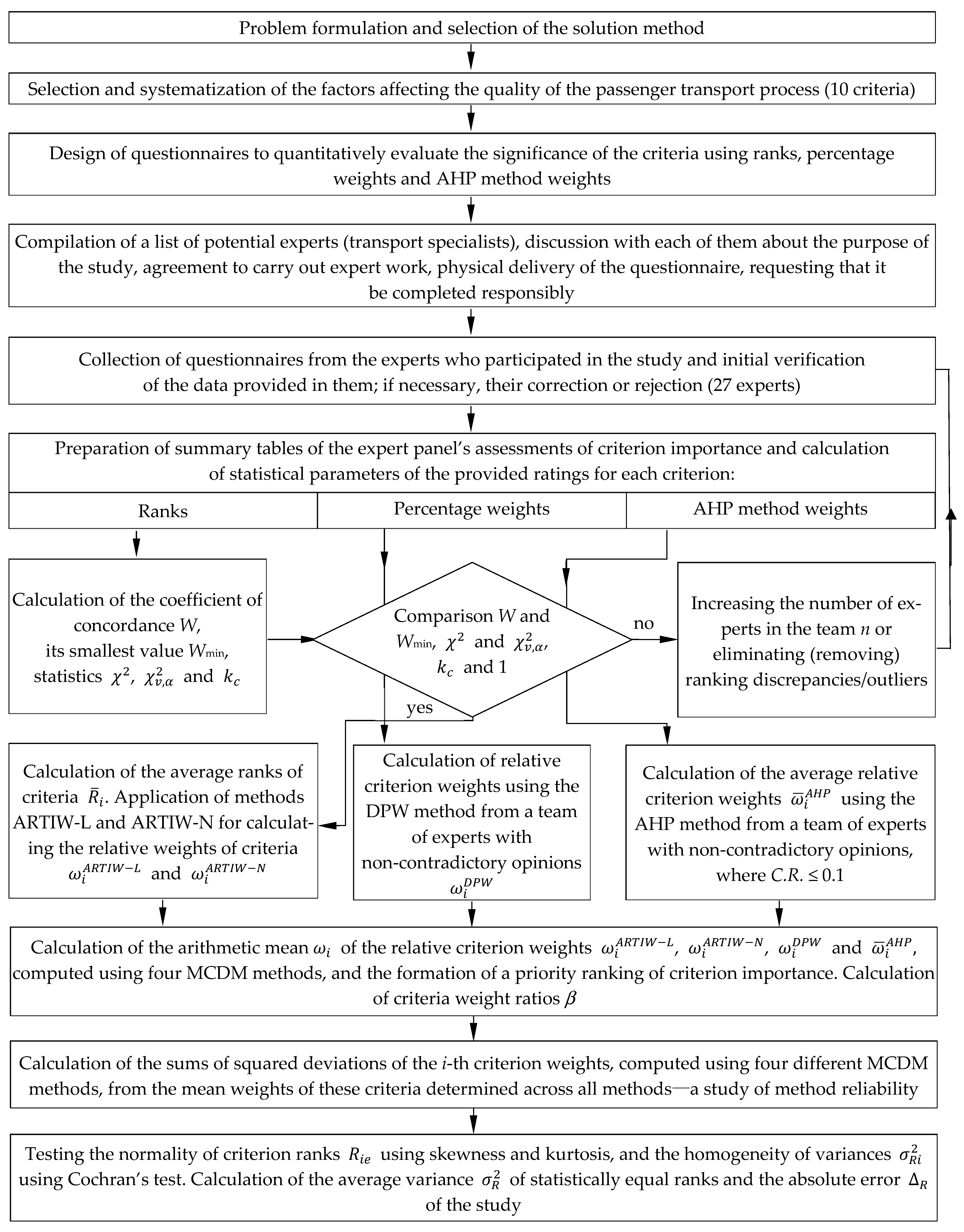
The research sequence (algorithm) is presented in Figure 1.

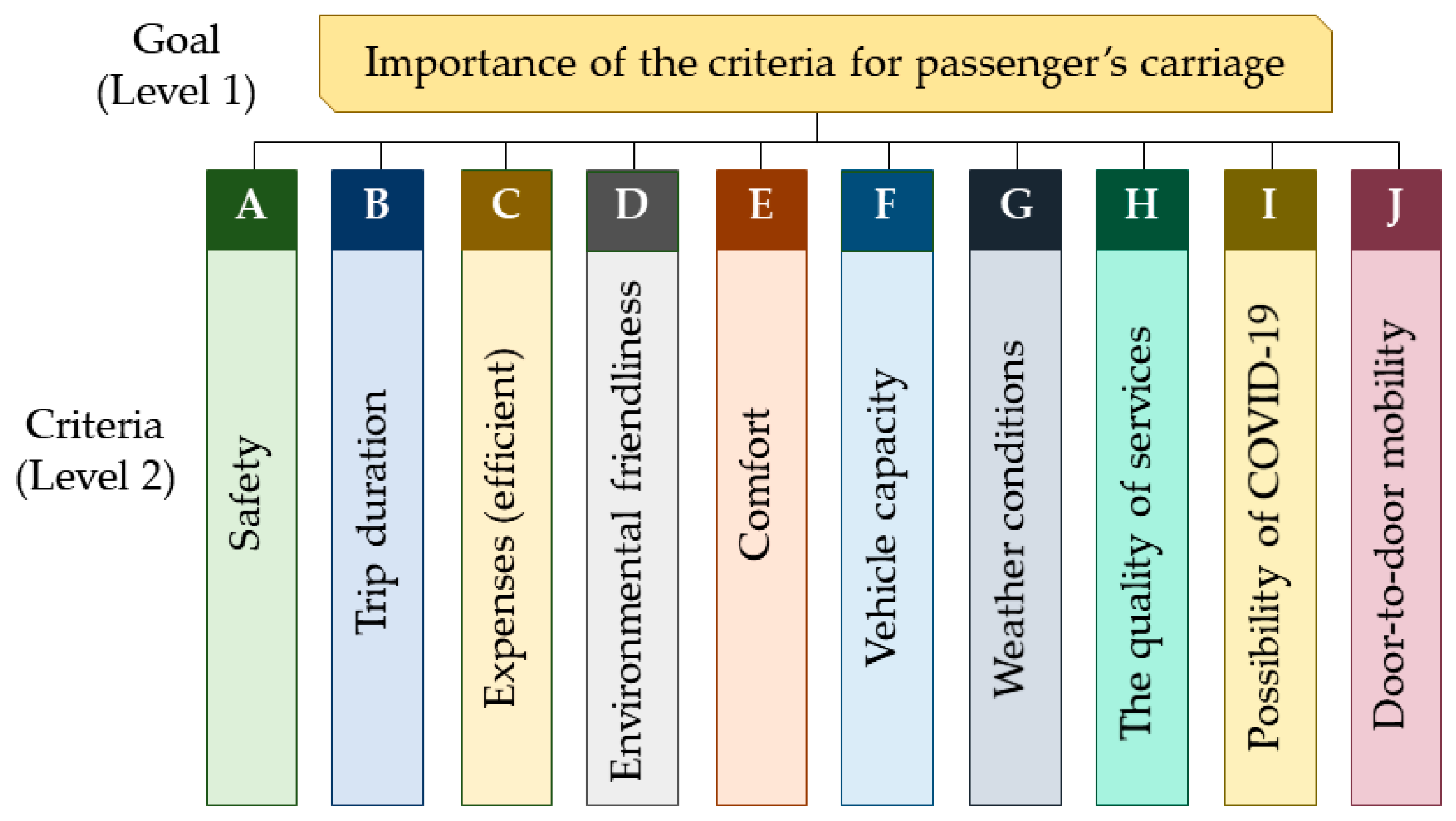
The characteristics of any form of public transport must be such that they improve the quality of travel. The most important characteristics (criteria) of passenger transport are presented in the model in Figure 2.

The principles of the significance analysis of these criteria, classified as Level 2, and the evaluation by a single expert using the AHP method are presented in a scientific monograph [5]. The assessment by a team of experts is more reliable than the opinion of a single expert. In addition, the use of several MCDM methods allows for a more accurate assessment of the importance of criteria. There is no universal questionnaire suitable for assessing the significance of the characteristics (criteria) of any object. Therefore, the authors of this study developed an expert questionnaire and administered it to the expert after obtaining his consent to participate in the assessment. The expert evaluated 10 independent criteria (Figure 2) using ranks, percentage weights, and the mutual intensity elements of the pairwise comparison matrix of the AHP method. Each questionnaire was reviewed by the researchers and, necessary, corrected in consultation with experts (most often, adjustments were required to the AHP matrix).

2.2. Experts

The authors’ long-standing academic research experience, as well as the practical experience of one of them in the transport sector, enabled engagement with experienced transport professionals and the utilization of their knowledge, competencies, and expertise for an objective assessment of the research subject. A list of potential experts was compiled, including specialists in road, rail and air transport. Each of them was then asked to participate in the study by completing a written questionnaire. Twenty-seven experts agreed to participate in the study, nine of whom hold PhDs. The team’s experts represented three fields (specializations) of transportation engineering: 17 from road transport, 6 from rail transport, and 4 from air transport. The evaluations of the criteria by each expert were given equal weight, with no preference given to any of them.

2.3. MCDM Methods Used to Analyze the Relevance of the Criteria

2.3.1. Principles and Ordering of Criterion Importance

By its very nature, every economic and social phenomenon is a complex phenomenon. None of them can be expressed by a single measure, indicator, or criterion, because it is difficult to identify a single characteristic that would encompass all the essential aspects of the phenomenon. Multi-criteria methods are used for the comprehensive evaluation of complex variables [39,40].

The team expert (e = 1, 2, …, n) was tasked with determining the differences in the characteristics of the object under study. To do so, they first ranked R_ie the objects in the questionnaire and assessed the importance of all criteria (i = 1, 2, …, m) on a scale from 1 (most important criterion) to 10 (least important criterion). There were no repeated ranks on the rank scale (order scale). The sum of the scores assigned to the criteria by the expert, as calculated by Formula (1), equals 55.

$${\sum }_{i=1}^m{R}_{ie}-{\displaystyle \frac{n\left(m+1\right)}{2}},$$

(1)

here, m is the number of criteria (i = 1, 2, …, m). In this study, m = 10.

After that, the expert assessed the significance of the criteria by assigning to them percentage weights P_ie—accurate to one hundredth or to a whole number—considering the priority of the criteria as determined by their rankings. The most important criterion was assigned the highest P_ie value, and the least important criterion was assigned the lowest P_ie value, with the total sum of all P_ie values equaling ${\sum }_{i=1}^m{P}_{ie}=100.0$%.

Finally, the expert used the nine-point fundamental scale of the AHP method [41] to compare the criteria in pairs, assigning them relative intensities of importance $a_{ji}=1/a_{ij}$ and filling out a reciprocal matrix $\mathit{A}={\left|a_{ij}\right|}_{m\times m}$. If the expert believes the two criteria under comparison are equally important, they will write in the relevant matrix cell $a_{ij}=1$. If the first criterion is slightly more important than the second criterion, then $a_{ij}=3$. If the first criterion is much more important than the second criterion, then $a_{ij}=5$. When the first criterion is significantly more important than the second criterion, then $a_{ij}=7$. When the first criterion is vastly more important than the second criterion, then $a_{ij}=9$. Some elements $a_{ij}$ of the matrix may be repeated. Even-numbered elements of matrix A are also possible ($a_{ij}$ = 2, 4, 6, 8). Before evaluating the importance of criteria in the matrix, it is recommended to list them in order of importance, from most to least important, and, while adhering to the transitivity condition, to compare the criterion in a row on the left side of the matrix with the criterion in the column above it. Each completed AHP matrix was checked. If any minor errors were found, the conflicting elements $a_{ij}$ were corrected without altering the ranking of the criteria.

2.3.2. Consistency of the Expert Panel’s Opinions

The averages of the quantitative significance estimates assigned to the criteria by the team of experts may be taken as the result of the problem-solving process only when the experts’ assessments are not contradictory, i.e., when their opinions are consistent. One of the most used measures of agreement for assessing the consistency of expert opinions to date has been Kendall’s coefficient of concordance W [42], which is calculated using Formula (2) when there are no tied ranks:

$$W={\displaystyle \frac{12S}{n^2\left(m^3-m\right)}},$$

(2)

where m is the number of passenger transport characteristics (criteria) being evaluated, i = 1, 2, …, m; n is the number of experts in the team who assessed the importance of the criteria, e = 1, 2, …, n; S is the sum of the squared deviations of all criteria rank sums ${\sum }_{e=1}^n{R}_{ie}$ from the overall mean rank $\overline{R}={\displaystyle \frac{1}{2}}n\left(m+1\right)$, calculated using Formula (3).

$$S={\sum }_{i=1}^m{\left({\displaystyle {\sum }_{e=1}^n}{R}_{ie}-\overline{R}\right)}^2.$$

(3)

When determining the consistency of the opinions of the team of experts, which are presented as rankings, Pearson’s chi-square statistic ${\chi }^2$ is calculated, which depends on the W value. Kendall [43] demonstrated that, when m > 7, the significance of the coefficient of concordance can be determined using a test ${\chi }^2$ involving a random variable calculated according to Formula (4):

$${\chi }^2={\displaystyle \frac{12S}{nm\left(m+1\right)}},$$

(4)

which is distributed according to a distribution ${\chi }^2$ with degrees of freedom $v=m-1$. Based on the significance level α, which in practice is usually set to $\alpha =0.05$ or $\alpha =0.01$, the critical value is found from the distribution table ${\chi }^2$ with degrees of freedom $v=m-1$. If the value ${\chi }^2$ calculated using Formula (4) is greater than the critical value ${\chi }_{v,\alpha }^2$, the experts’ assessments are in agreement.

The consistency of the team of experts’ opinions can be determined using a direct method [44] by comparing the value of W with the critical value of the concordance coefficient $W_{\mathrm{m}\mathrm{i}\mathrm{n}}$, calculated from Formula (5):

$$W_{min}={\displaystyle \frac{{\chi }_{v,\alpha }^2}{n\left(m-1\right)}}.$$

(5)

The degree of opinion compatibility is indicated by the value of the compatibility coefficient $k_c$ calculated by Formula (6) [45]:

$$k_c={\displaystyle \frac{{\mathsf{\chi }}^2}{{\chi }_{v,\alpha }^2}}={\displaystyle \frac{W}{W_{\mathrm{m}\mathrm{i}\mathrm{n}}}}.$$

(6)

When the experts’ opinions on the importance of a criterion, expressed in terms of their rankings, are consistent, they are $k_c>1$ and the higher the value, the more consistent the experts’ opinions are (the closer they are to one another).

2.3.3. The ARTIW-L Method for Calculating the Relative Weights of Criteria

Various methods (algorithms) can be used to determine the relative weights of the ranked indicators and characteristics (criteria), none of which has a theoretical advantage over the others. The general principle of all algorithms is the same—the most important criterion should be given the highest weight. The weights must correspond to the ranks (importance) of the indicators, and their sum must equal one; that is, the weights are normalized [46].

The relative weights of the criteria can be calculated from their ranks using the ARTIW-L (average rank transformation into weight-linear) and ARTIW-N (average rank transformation into weight non-linear) methods [47].

The relative weight ${\omega }_i^{ARTIW-L}$ of the i-th criterion is calculated using the ARTIW-L method according to Formula (7):

$${\omega }_i^{ARTIW-L}={\displaystyle \frac{m-{\overline{R}}_i+1}{{\displaystyle {\sum }_{i=1}^m}{\overline{R}}_i}},$$

(7)

here—${\overline{R}}_i$ is the mean of the ranks ${\overline{R}}_i={\sum }_{e=1}^n{R}_{ie}:n$ for the i-th criterion, calculated from the evaluations of a team of n experts.

2.3.4. The ARTIW-N Method for Calculating the Relative Weights of Criteria

The ranks of a criterion can be used to calculate its relative weight ${\omega }_i^{ARTIW-N}$ using the ARTIW-N method. To do this, first, according to Formula (8), the ratio of the mean rank $\underset{i}{\min }{\overline{R}}_i$ of the most important criterion to the average rank of each i-th criterion ${\overline{R}}_i$ is calculated

$$u_i={\displaystyle \frac{\underset{i}{\min }{\overline{R}}_i}{{\overline{R}}_i}}.$$

(8)

The weight of each criterion $u_i$ is normalized using the Formula (9) as follows ${\omega }_i^{ARTIW-N}$:

$${\omega }_i^{ARTIW-N}={\displaystyle \frac{u_i}{{\displaystyle {\sum }_{i=1}^m}{u}_i·}}.$$

(9)

The criterion weights ${\omega }_i^{ARTIW-L}$ calculated using the ARTIW-L method are linearly inversely related to the mean ranks of the criteria ${\overline{R}}_i$. The criterion weights ${\omega }_i^{ARTIW-N}$ calculated using the ARTIW-N method are linked to the mean ranks of these criteria ${\overline{R}}_i$ via a curvilinear (nonlinear) inverse functional relationship.

2.3.5. The DPW Method for Calculating the Relative Weights of Criteria

The significance of the i-th criteria (i = 1, 2, …, m), assessed in percentage weights P_ie by each e-th expert (e = 1, 2, …, n), was used in applying the DPW method to calculate the average relative weight of the criterion according to Formula (10):

$${\omega }_i^{DPW}={\displaystyle \frac{{\sum }_{e=1}^n{P}_{ie}}{100n}}.$$

(10)

This method is just as clear and logical as the method of ranking indicators (criteria). However, it is more accurate. The significances of the criteria assessed using the DPW method not only indicate that one criterion is more important than another (as rankings also show $R_{ie}$), but also how much more important it is, since $P_{ie}$ can be expressed with an accuracy of one tenth of a percent, and the difference between two adjacent criteria $P_{ie}$usually varies from 0.1 to 1 or more. The relative weights ${\omega }_i^{DPW}$ of the criteria calculated using the DPW method are linked to the mean ranks of the criteria ${\overline{R}}_i$ by an inverse curvilinear correlation.

2.3.6. The AHP Method for Calculating the Relative Weights of Criteria

From the elements $a_{ij}$ of the pairwise comparison matrix of criteria $\mathit{A}={\left|a_{ij}\right|}_{m\times m}$, completed by the e-th expert using the AHP method, the eigenvector was calculated according to Formula (11):

$${\omega }_{ie}^{AHP}={\displaystyle \frac{\sqrt[m]{{\displaystyle {\prod }_{j=1}^m}{a}_{ij}}}{{\displaystyle {\sum }_{i=1}^m}\sqrt[m]{{\displaystyle {\prod }_{j=1}^m}{a}_{ij}}}}.$$

(11)

The elements $a_{ij}$ of matrix A can be taken as the ratios of the values of two compared indicators $C_i$ and $C_i$ and after normalizing these values, as the relative weights of the indicators (criteria).

The average weight ${\overline{\omega }}_i^{AHP}$ of each evaluated criterion was calculated by the expert team using Formula (12):

$${\overline{\omega }}_i^{AHP}={\displaystyle \frac{{\sum }_{e=1}^n{\omega }_{ie}^{AHP}}{n}}.$$

(12)

Whether each matrix completed by an expert is correct (consistent) was determined using Formula (13) by calculating the consistency index $C.I.$:

$$C.I.={\displaystyle \frac{{\lambda }_{\mathrm{m}\mathrm{a}\mathrm{x},e}-m}{m-1}},$$

(13)

here, ${\lambda }_{\mathrm{m}\mathrm{a}\mathrm{x},e}$ is the largest eigenvalue of matrix A of the e-th expert, calculated using Formula (14).

$${\lambda }_{\mathrm{m}\mathrm{a}\mathrm{x},e}={\displaystyle \frac{1}{m}}{\displaystyle {\sum }_{i=1}^m}{\displaystyle \frac{{\displaystyle {\sum }_{j=1}^m}{a}_{ij}{\omega }_{ie}^{AHP}}{{\omega }_{ie}^{AHP}}}.$$

(14)

The ratio of the consistency index $C.I.$ to the random index $R.I.$ is called the consistency ratio $C.R.$ The value of the random index $R.I.$, which depends on the size of the matrix m, is obtained from a table [41]. Since 10 criteria are compared in this study (m = 10), then R.I. = 1.49.

The matrix is considered consistent if C.R. $\le$ 0.1, which allows its eigenvector ${\omega }_{ie}^{AHP}$ to be regarded as a justified relative weight of the criterion [48,49]. When $C.R.\le 0.1$, the consistency of matrix A is considered acceptable. In this situation, the weight of the indicator calculated using this matrix has a high reliability. When $C.R.>0.1$, the judgment matrix does not satisfy the consistency requirements and must be revised to ensure the credibility of the weight [50]. In some studies [51], it is stated that the resulting vector is accepted if the consistency ratio is about 0.10 or less (0.20 may be tolerated, but not more). Other researchers [52,53,54] do not calculate the matrix $C.R.$ and do not assess its consistency.

2.3.7. The Use of the Average of Four MCDM Methods for Calculating the Relative Weights of Criteria

A combination of subjective and objective methods was used for weighting to ensure the scientific and effective selection of the optimal scheme. Road-related factors and climate indicators were incorporated into the entropy method for objective weighting [49].

To increase the reliability of the evaluation results of the object under study (passenger transport characteristics), it is recommended [39] to apply several MCDM methods simultaneously. The agreement (similarity) of all or most results reduces the likelihood of making an incorrect decision.

The average relative weight of each criterion ${\omega }_i$ determined using the four methods applied in this study is calculated according to Formula (15) [55]:

$${\omega }_i={\displaystyle \frac{{\displaystyle {\sum }_{k=1}^r}{\omega }_{ik}}{r}},$$

(15)

here, ${\omega }_{ik}$ is the relative weight of the i-th criterion calculated using the k-th MCDM method (k = 1, 2, …, r), and r is the number of methods used in the study.

Finally, the relative weight ${\omega }_i^{\prime }$ of the more important criterion is compared with the relative weight ${\omega }_i^{″}$ of the less important criterion by calculating their ratio β according to Formula (16):

$$\beta ={\displaystyle \frac{{\omega }_i^{\prime }}{{\omega }_i^{″}}}.$$

(16)

Assuming that a sample of size r is drawn from a population with a distribution close to normal, the standard deviation ${\widehat{S}}_{i\omega }$ can be estimated from the range of the data set $R_{i\omega }$ [50]. The relative weight of each criterion calculated using different MCDM methods varies. This difference was assessed by calculating the standard deviation ${\widehat{S}}_{i\omega }$ from the range of the relative weight data set $R_{i\omega }$ according to Formula (17):

$${\widehat{S}}_{i\omega }=R_{i\omega }\times {\displaystyle \frac{1}{d_n}}={\displaystyle \frac{{\omega }_{i\mathrm{m}\mathrm{a}\mathrm{x}}-{\omega }_{i\mathrm{m}\mathrm{i}\mathrm{n}}}{K}},$$

(17)

here, ${\omega }_{i\mathrm{m}\mathrm{a}\mathrm{x}}$ and ${\omega }_{i\mathrm{m}\mathrm{i}\mathrm{n}}$ are the maximum and minimum values of the average relative weight of the i-th criterion calculated using all MCDM methods; 1/$d_n$ and $K$ are, respectively, the multiplier and the coefficient used to estimate the approximate standard deviation, depending on the number of MCDM methods applied r. When r = 4, the multiplier is 1/$d_n=0.4857$ [56], and the coefficient is $d_n=$ 2.06 [57].

By dividing the standard deviation ${\widehat{S}}_{i\omega }$ of the average relative weights of each criterion by the mean weight of the criterion ${\omega }_i$, the percentage coefficient of variation of the relative weights for each criterion was calculated according to Formula (18):

$$V_{i\omega }={\displaystyle \frac{{\widehat{S}}_{i\omega }}{{\omega }_i}}100.$$

(18)

The absolute error ${∆}_R$ of the research data is calculated based on the sample size according to Formula (19) [58,59]:

$${∆}_R=\sqrt{{\displaystyle \frac{t^2\times {\sigma }_R^2}{n}}},$$

(19)

here, t is Student’s test coefficient corresponding to the probability of obtaining the error within specified limits (at probability P = 95%, t = 1.96); n is the number of experts in the team; and ${\sigma }_R$ is the average of the standard deviations of the ranks of the criteria comprising the object under study.

The acceptable margin of error for the estimated mean ${∆}_R$ [60] largely depends on the magnitude of the variance ${\sigma }_R^2$, which indicates the degree of dispersion (spread, variability) of the ranks of all criteria. When the calculated variances ${\sigma }_{Ri}^2$ of the ranks of all criteria are statistically equal, and the dispersion of the ranks follows a normal distribution, the mean variance of the ranks of all criteria of the object under study is calculated using Formula (20):

$${\sigma }_R^2={\displaystyle \frac{{\sum }_{i=1}^m{\sigma }_{Ri}^2}{m}}.$$

(20)

The equality of variances ${\sigma }_{Ri}^2$ is tested using Cochran’s test [56], since their values are calculated from samples of equal size n that follow a normal distribution. Cochran’s statistic ${\widehat{G}}_{\mathrm{m}\mathrm{a}\mathrm{x}}$ is calculated according to Formula (21):

$${\widehat{G}}_{\mathrm{m}\mathrm{a}\mathrm{x}}={\displaystyle \frac{\underset{i}{\max } {\sigma }_{Ri}^2}{{\sum }_{i=1}^m{\sigma }_{Ri}^2}},$$

(21)

here, $\underset{i}{\max } {\sigma }_{Ri}^2$ is the largest variance of the ranks calculated from all m criteria.

The calculated value for the equality of variances ${\widehat{G}}_{\mathrm{m}\mathrm{a}\mathrm{x}}$ must be less than its critical value $G_c\left(\alpha ;m;v\right)$, which depends on the significance level α, the number of criteria m, and the degrees of freedom $v=n-1$.

The conformity of the variation of criterion ranks $R_{ie}$ to a normal distribution is indicated by the skewness (Sk) and kurtosis (Ku) of the ranks. The closer they are to zero, the more closely the distribution conforms to the normal distribution law. Due to the limited sample size n, the absolute values of |Sk| and |Ku| may be greater than zero. For a normal distribution, (|Sk|) and (|Ku|) must be smaller than their standard deviations, $s_{Sk}$ and $s_{Ku}$, multiplied by 3 and 5, respectively, i.e., $\left|Sk\right|\le 3s_{Sk}$ and $\left|Ku\right|\le 5s_{Ku}$ [47].

2.3.8. Limitations

Passenger transportation belongs to the category of complex systems that cannot be expressed by a single measure, indicator, or criterion, as it is difficult to identify a single characteristic that would encompass all essential aspects of this process. The properties of passenger transport are of varying importance when selecting a mode of travel. The significance of these properties (criteria) can be quantitatively determined and evaluated using MCDM methods by drawing on the competence, knowledge, and expertise of specialists (experts). The most commonly used expert-based methods for directly determining indicator (criterion) weights involve pairwise comparisons of criteria. These include ranking, ARTIW-L, ARTIW-N, DPW, and AHP methods, which are widely used in scientific research. The importance assigned to criteria by different expert panels may vary; however, only an adequate level of agreement among experts allows the average ranking to be considered reliable. All expert opinions are treated as equally important, without assigning preference to any individual. None of the MCDM methods has a theoretical advantage over the others. To increase the reliability of passenger transport assessment results, several MCDM methods are applied simultaneously. Among the MCDM methods applied in this study, the most reliable is considered to be the one that produces the smallest sum of squared deviations between its calculated criterion weights and the mean weights obtained across all methods.

3. Results and Discussion

3.1. Consistency of the Opinion of the Team of Experts

The data on the significance of passenger transport characteristics (criteria), as ranked by the expert team, are presented in

Table 1. The significance of passenger transport characteristics in selecting the mode (means) of travel, as determined by the expert team using the ARTIW-L and ARTIW-N methods.

Method and Formula	Property (Indicator, Criterion); i = 1, 2, …, m										Total
	A	B	C	D	E	F	G	H	I	J
${\sum }_{e=1}^n{R}_{ie}$	43	83	79	181	109	198	206	197	235	154	1485
${\overline{R}}_i={\sum }_{e=1}^n{R}_{ie}/n$	1.593	3.074	2.926	6.704	4.037	7.333	7.629	7.296	8.704	5.704	55
${\sum }_{e=1}^n{R}_{ie}-{\displaystyle \frac{n\left(m+1\right)}{2}}$	−105.5	−65.5	−69.5	32.5	−39.5	49.5	57.5	48.5	86.5	5.5	0.0
${\left[{\sum }_{e=1}^n{R}_{ie}-{\displaystyle \frac{n\left(m+1\right)}{2}}\right]}^2$	11,130	4290	4830	1057	1560	2450	3306	2353	7482	30	38,488
${\sigma }_{Ri}=\sqrt{{\displaystyle \frac{{\sum }_{e=1}^n{\left(R_{ie}-{\overline{R}}_i\right)}^2}{n-1}}}$	1152	1542	1328	2383	1629	2112	1445	1728	1772	2090	-
Skewness (Sk)	2.53	0.55	1.10	−0.48	0.17	−0.32	−0.36	−0.35	−1.44	0.07	-
Kurtosis (Ku)	7.49	−0.52	0.40	−0.58	0.22	−1.23	−0.07	−0.73	1.18	0.01	-
ARTIW-L method:
${\omega }_i^{ARTIW-L}={\displaystyle \frac{m+1-{\overline{R}}_i}{{\sum }_{i=1}^m{\overline{R}}_i}}$	0.1710	0.1441	0.1468	0.0781	0.1266	0.0667	0.0613	0.0674	0.0417	0.0963	1.0000
Priority	1	3	2	6	4	8	9	7	10	5	55
ARTIW-N method:
$u_i={\displaystyle \frac{\underset{i}{\min } {\overline{R}}_i}{{\overline{R}}_i}}$	1	0.5182	0.5444	0.2376	0.3946	0.2172	0.2088	0.2183	0.1830	0.2793	3.8014
${\omega }_i^{ARTIW-N}={\displaystyle \frac{u_i}{{\sum }_{i=1}^m{u}_i}}$	0.2631	0.1363	0.1432	0.0625	0.1038	0.0571	0.0549	0.0574	0.0482	0.0735	1.0000
Priority	1	3	2	6	4	8	9	7	10	5	55

. From the mean ${\overline{R}}_i$ of the sum of ranks ${\sum }_{e=1}^n{R}_{ie}$ for each criterion and the overall mean rank $\overline{R}$, the sum of squared deviations was calculated according to Formula (3), yielding S = 38488. By substituting this value into Formula (2), the consistency of the expert team’s opinions was evaluated, as indicated by Kendall’s coefficient of concordance:

$$W={\displaystyle \frac{12·38488}{{27}^2\left({10}^3-10\right)}}=0.64.$$

The significance of Kendall’s coefficient of concordance W was evaluated by calculating the chi-square random variable of Pearson’s chi-square distribution ${\chi }^2$ according to Formula (4):

$${\chi }^2={\displaystyle \frac{12·S}{nm\left(m+1\right)}}={\displaystyle \frac{12·38488}{27·10\left(10+1\right)}}=155.5.$$

The chi-square statistic was compared with its critical value ${\chi }_{v,\alpha }^2$, which depends on the degrees of freedom $v=m-1=10-1=9$ and the chosen significance level $\alpha =0.05$. The critical value given in the table [61] is equal to ${\chi }_{9;0.05}^2=16.92$.

The calculated minimum threshold value $W_{min}$, which depends on ${\chi }_{v,\alpha }^2$, n, and m, is equal to:

$$W_{\mathrm{m}\mathrm{i}\mathrm{n}}={\displaystyle \frac{{\chi }_{v,\alpha }^2}{n\left(m-1\right)}}={\displaystyle \frac{16.92}{27\left(10-1\right)}}=0.0696.$$

From the ratio of the chi-square statistic obtained from the ranks ${\chi }^2$to its critical value ${\chi }_{v,\alpha }^2$, and the ratio of the empirical coefficient of concordance W to its minimum value $W_{min}$, the compatibility coefficient was determined according to Formula (6) as follows:

$$k_c={\displaystyle \frac{{\mathsf{\chi }}^2}{{\chi }_{v,\alpha }^2}}={\displaystyle \frac{W}{W_{\mathrm{m}\mathrm{i}\mathrm{n}}}}={\displaystyle \frac{155.5}{16.92}}={\displaystyle \frac{0.64}{0.0696}}=9.19.$$

It shows that the opinions of the expert team in evaluating the significance of passenger transport characteristics when selecting the mode of travel are highly consistent (non-contradictory). This allows the arithmetic means of the criterion ranks and other significance estimates to be used as reliable solutions to the problem.

3.2. The Relative Weights of the Criteria Calculated Using the ARTIW-L Method

The mean rank of each criterion ${\overline{R}}_i$was used to calculate the relative weight of the criterion by applying Formula (7) according to the ARTIW-L method. The relative weight of the first criterion is equal to:

$${\omega }_A^{ARTIW-L}={\displaystyle \frac{m-{\overline{R}}_A+1}{{\displaystyle {\sum }_{i=1}^m}{\overline{R}}_i}}={\displaystyle \frac{10-1.593+1}{55}}=0.1710.$$

The relative weights ${\omega }_i^{ARTIW-L}$ and priorities of all criteria are presented in Table 1. They show that the most important is criterion A (safety), while the least important is criterion I (possibility of COVID-19), and the ratio of their relative weights is β = 4.1.

3.3. The Relative Weights of the Criteria Calculated Using the ARTIW-N Method

The results of calculating the relative weights of the criteria ${\omega }_i^{ARTIW-N}$ using the ARTIW-N method are presented in Table 1. Initially, the smallest mean rank of the criteria $\underset{i}{\min } {\overline{R}}_i$was divided by the mean rank of each criterion ${\overline{R}}_i$. After that, their ratio $u_i$ was normalized. The value for the first criterion A $u_A$ (the most important one), calculated according to Formula (8), is equal to:

$$u_A={\displaystyle \frac{\underset{i}{\min } {\overline{R}}_i}{{\overline{R}}_A}}={\displaystyle \frac{1.593}{1.593}}=1.$$

After normalizing it according to Formula (9), the relative weight ${\omega }_A^{ARTIW-L}$ of criterion A is equal to:

$${\omega }_A^{ARTIW-N}={\displaystyle \frac{u_A}{{\displaystyle {\sum }_{i=1}^m}{u}_i·}}={\displaystyle \frac{1}{3.8014}}=0.2631.$$

The relative weights ${\omega }_i^{ARTIW-N}$and priorities of all 10 criteria are presented in Table 1. The relative weight of the most important criterion A (safety) is β = 5.5 times greater than the relative weight of the least important criterion I (possibility of COVID-19).

The relative weights of the criteria calculated using the ARTIW-L and ARTIW-N methods differ slightly. However, the ranking order of the criteria, from the most important to the least important is the same: A > C > B > E > J > D > H > F > G > I.

3.4. The Relative Weights of the Criteria Calculated Using the DPW Method

The sum of the significances of all 10 criteria, assessed as percentage weights ${\sum }_{e=1}^n{P}_{ie}$, their standard deviations ${\sigma }_{P_i}$, skewness, kurtosis, relative weights ${\omega }_i^{DPW}$ and priorities are presented in

Table 2. The significance of passenger transport characteristics in selecting the mode (means) of travel, as determined by the expert team using the DPW method.

Method and Formula	Property (Indicator, Criterion); i = 1, 2, …, m										Total
	A	B	C	D	E	F	G	H	I	J
${\sum }_{e=1}^n{P}_{ie}$	567	391.5	380	189	336.3	176.9	152.2	158.6	108.5	240	2700
${\overline{P}}_i={\sum }_{e=1}^n{P}_{ie}/n$	21.0	14.5	14.07	7.0	12.46	6.55	5.64	5.87	4.02	8.89	100.00
${\sigma }_{Pi}=\sqrt{{\displaystyle \frac{{\sum }_{e=1}^n{\left(P_{ie}-{\overline{P}}_i\right)}^2}{n-1}}}$	11.077	4631	3551	4481	5883	3452	2723	2969	2559	4003	-
Skewness (Sk)	2.99	0.82	−0.34	0.66	1.93	0.13	0.22	0.04	0.82	0.40	-
Kurtosis (Ku)	10.08	1.29	−0.86	−0.49	7.99	−0.93	−0.19	−0.68	0.63	−0.12	-
DPW method:
${\omega }_i^{DPW}={\displaystyle \frac{{\sum }_{e=1}^n{P}_{ie}}{100n}}$	0.2100	0.1450	0.1407	0.0700	0.1246	0.0655	0.0564	0.0587	0.0402	0.0889	1.0000
Priority	1	2	3	6	4	7	9	8	10	5	55

.

The relative weight of criterion A, calculated according to Formula (10), is equal to:

$${\omega }_A^{DPW}={\displaystyle \frac{{\sum }_{e=1}^n{P}_{Ae}}{100n}}={\displaystyle \frac{567}{100·27}}=0.2100.$$

The relative weight ${\omega }_A^{DPW}$ of the most important criterion A (safety) is β = 5.2 times greater than the relative weight ${\omega }_I^{DPW}$ of the least important criterion I. The relative weights ${\omega }_i^{DPW}$ made it possible to establish the priority order of the criteria—from the most important to the least important—which is as follows: A > B > C > E > J > D > F > H > G > I. It differs slightly from the priority order of the criteria determined using the ARTIW-L and ARTIW-N methods: the priorities of criteria C and B were 2 and 3, respectively, while those of H and F were 7 and 8, respectively. According to the DPW method, the priorities of these criteria (C and B) are 3 and 2, respectively, while those of criteria H and F priorities are 8 and 7, respectively, i.e., their positions have been reversed.

3.5. The Relative Weights of the Criteria Calculated Using the AHP Method

Each expert independently (voluntarily) completed the reciprocal matrix of the AHP method by comparing the 10 criteria in pairs. The sum ${\sum }_{e=1}^n{\omega }_{ie}^{AHP}$ and mean ${\overline{\omega }}_i^{AHP}$ of the eigenvectors of the matrices of all 27 experts, along with their standard deviations ${\sigma }_{\omega i}^{AHP}$, skewness, kurtosis, and priorities, are presented in

Table 3. The significance of passenger transport characteristics in selecting the mode (means) of travel, as determined by the expert team using the AHP method.

Method and Formula	Property (Indicator, Criterion); i = 1, 2, …, m										Total
	A	B	C	D	E	F	G	H	I	J
${\omega }_{ie}^{AHP}={\displaystyle \frac{\sqrt[m]{{\displaystyle {\prod }_{j=1}^m}{a}_{ij}}}{{\displaystyle {\sum }_{i=1}^m}\sqrt[m]{{\displaystyle {\prod }_{j=1}^m}{a}_{ij}}}}$	From the elements of the pairwise comparison matrix $a_{ij}$ completed by each expert, the eigenvector (relative weight) of the i-th criterion is calculated ${\omega }_{ie}^{AHP}$. Each matrix must be consistent (C.R. < 0.1).
${\sum }_{e=1}^n{\omega }_{ie}^{AHP}$	6.743	4.339	4.441	1.710	3.171	1.337	1.084	1.211	0.804	2.160	27.000
${\overline{\omega }}_i^{AHP}={\sum }_{e=1}^n{\omega }_{ie}^{AHP}/n$	0.2497	0.1607	0.1645	0.0633	0.1174	0.0495	0.0402	0.0449	0.0298	0.0800	1.0000
${\sigma }_{{\omega }_i}^{AHP}=\sqrt{{\displaystyle \frac{{\sum }_{e=1}^n{\left({\omega }_{ie}^{AHP}-{\overline{\omega }}_i^{AHP}\right)}^2}{n-1}}}$	0.070	0.068	0.055	0.056	0.056	0.034	0.024	0.028	0.026	0.051	-
Skewness (Sk)	−0.97	0.35	−0.45	1.71	1.26	0.88	2.30	1.46	2.20	1.06	-
Kurtosis (Ku)	1.12	−0.33	−0.79	2.72	2.24	−0.52	7.92	2.00	4.52	1.22	-
Priority	1	3	2	6	4	7	9	8	10	5	55

.

The consistency ratios of all matrices $C.R.$ ranged from 0.016 to 0.101, i.e., they are consistent (non-contradictory). Therefore, the eigenvector of each criterion ${\omega }_{ie}^{AHP}$ calculated according to Formula (11) is reasonably taken as the normalized relative weight of the criterion.

The mean relative weights ${\overline{\omega }}_i^{AHP}$ assigned by all experts for each criterion show that, according to the AHP method, the relative weight of the most important criterion A (safety) is β = 8.4 times greater than that of the least important criterion I (possibility of COVID-19). This method yielded the largest difference in the significance of the criteria when compared with the significances calculated using the ARTIW-L, ARTIW-N, and DPW methods. The relative weights of the criteria calculated using the AHP method indicate the following priority order of the criteria: A > C > B > E > J > D > F > H > G > I. The priority order of the six most important and the two least important criteria is the same as the order determined using the ARTIW-L and ARTIW-N methods. Only the priorities of criteria F and H differ: they were 8 and 7, whereas according to the AHP method they are 7 and 8. A comparison of the criteria priorities determined using the AHP and DPW methods shows that the order of most criteria is the same, except for criteria B and C, whose priorities were 2 and 3 (DPW) but became 3 and 2 (AHP).

3.6. Comparative Analysis of the Relative Weights of Criteria Calculated Using Four MCDM Methods

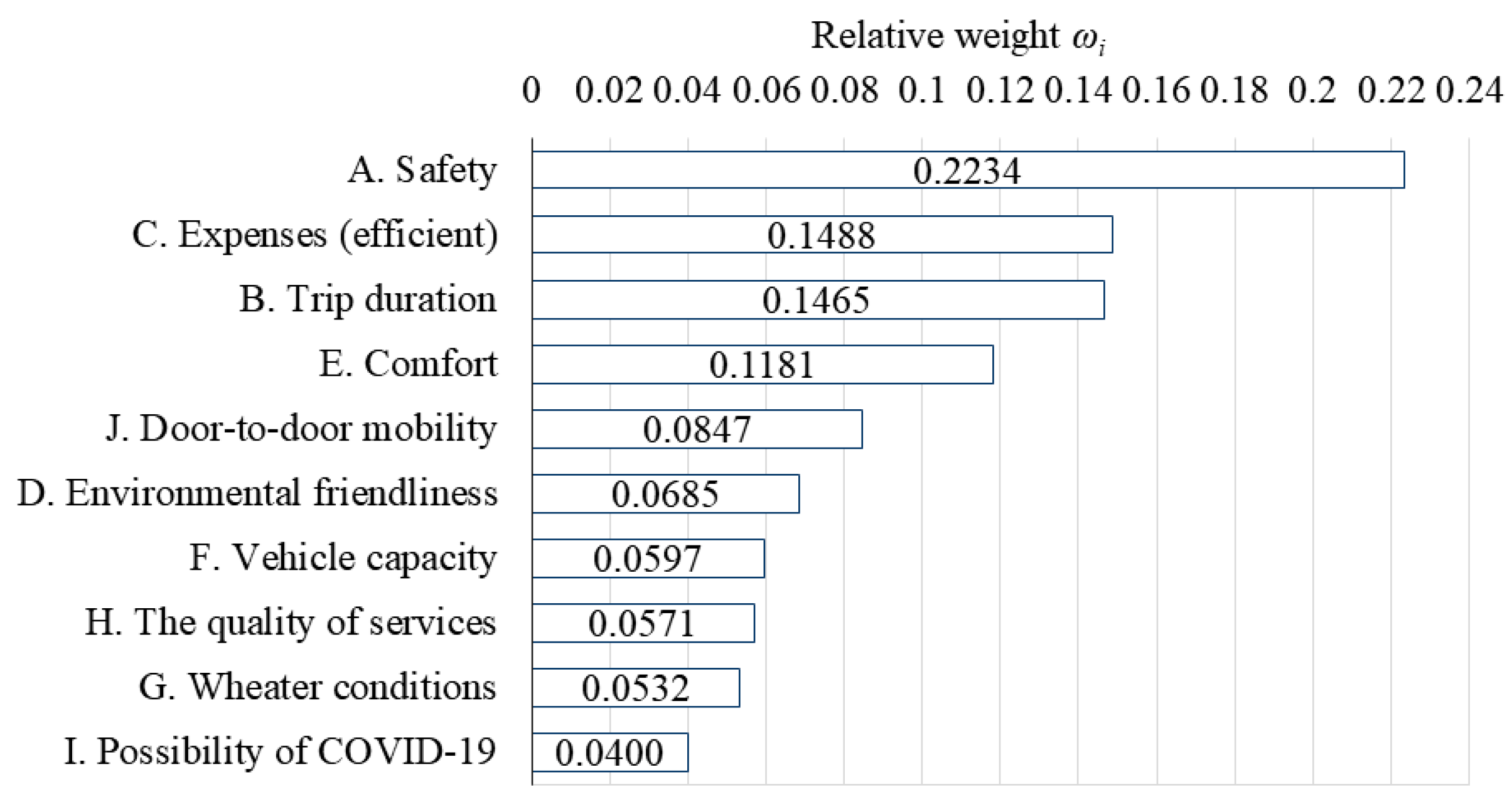
A comparative analysis of the relative weights of all criteria was carried out using the data presented in

Table 4. The significance of passenger transport characteristics in selecting the mode of travel, as determined by the expert team using the ARTIW-L, ARTIW-N, DPW and AHP methods.

Method Used for Calculation of Relative Weight of Criterion	Property (Indicator, Criterion); i = 1, 2, …, m										Total
	A	B	C	D	E	F	G	H	I	J
${\omega }_i^{ARTIW-L}$	0.1710	0.1441	0.1468	0.0781	0.1266	0.0667	0.0613	0.0674	0.0417	0.0963	1.0000
${\omega }_i^{ARTIW-N}$	0.2631	0.1363	0.1432	0.0625	0.1038	0.0571	0.0549	0.0574	0.0482	0.0735	1.0000
${\omega }_i^{DPW}$	0.2100	0.1450	0.1407	0.0700	0.1246	0.0655	0.0564	0.0587	0.0402	0.0889	1.0000
${\overline{\omega }}_i^{AHP}$	0.2497	0.1607	0.1645	0.0633	0.1174	0.0495	0.0402	0.0449	0.0298	0.0800	1.0000
Average of four methods ${\omega }_i$	0.2234	0.1465	0.1488	0.0685	0.1181	0.0597	0.0532	0.0571	0.0400	0.0847	1.0000
Priority	1	3	2	6	4	7	9	8	10	5	55
${\widehat{S}}_{i\omega }={\displaystyle \frac{{\omega }_{i\mathrm{m}\mathrm{a}\mathrm{x}}-{\omega }_{i\mathrm{m}\mathrm{i}\mathrm{n}}}{K}}$	0.0447	0.0118	0.0115	0.0076	0.0111	0.0083	0.0102	0.0110	0.0089	0.0111	-
$V_{i\omega }={\displaystyle \frac{{\widehat{S}}_{i\omega }}{{\omega }_i}}100\%$	20.0	8.1	7.7	11.1	9.4	13.9	19.2	19.3	22.2	13.1	-

. The average of the relative weights ${\omega }_i$calculated using four MCDM methods ranges from 0.2234 for the safety criterion A to 0.0400 for criterion I (risk of contracting COVID-19), i.e., they differ by approximately β = 5.6 times.

Whether the relative weights of each criterion ${\omega }_i^{ARTIW-L}$, ${\omega }_i^{ARTIW-N}$, ${\omega }_i^{DPW}$ and ${\overline{\omega }}_{{\omega }_i}^{AHP}$ determined by different MCDM methods differ significantly was assessed using the coefficient of variation (expressed as a percentage) $V_{i\omega }$. The standard deviations ${\widehat{S}}_{i\omega }$ and coefficients of variation $V_{i\omega }$, calculated from the ranges of the criteria’s relative weights $R_{i\omega }={\omega }_{i\mathrm{m}\mathrm{a}\mathrm{x}}-{\omega }_{i\mathrm{m}\mathrm{i}\mathrm{n}}$ using Formulas (17) and (18), are presented in Table 4.

The coefficient of variation of the relative weights ranges from 7.7% for criterion C to 22.2% for criterion I. The smaller the coefficient $V_{i\omega }$, the closer the relative weights of a criterion calculated by different methods are to each other. The dispersion of variable values is generally considered low when the coefficient of variation ranges from 0 to 10%, moderate from 10 to 20%, and high when it exceeds 20% [57]. In this study, the dispersion of significance is low for three criteria (C, B, E), moderate for six criteria (A, D, F, G, H, J), and high for one criterion (I).

Among the multiple MCDM methods applied in this study, the most reliable is considered to be the one that yields the smallest sum of squared deviations between its criterion weights and the mean criterion weights calculated across all methods. This is analogous to a sample: the reliability of a sample is higher than that of any individual sample unit comprising it. The relative criterion weights obtained using different methods, together with their mean values, are presented in

Table 5. The squares ${∆{\omega }_i}^2$ of the differences $∆{\omega }_i$ between the relative weights of the criteria calculated using different MCDM methods and the average relative weights of these criteria obtained from the four methods.

Method	Difference	Property (Criterion) i = 1, 2, …, m										Total
		A	B	C	D	E	F	G	H	I	J
ARTIW-L	$∆{\omega }_i$	−0.0524	−0.0024	−0.0020	0.0096	0.0085	0.0070	0.0081	0.0103	0.0017	0.0116	0
	$∆{\omega }_i^2$	0.00274	0.00001	0.00001	0.00009	0.00007	0.00005	0.00007	0.00011	0.00001	0.00013	0.00329
ARTIW-N	$∆{\omega }_i$	0.0397	−0.0102	−0.0056	−0.0060	−0.0143	−0.0026	0.0017	0.0003	0.0082	−0.0112	0
	$∆{\omega }_i^2$	0.00158	0.00010	0.00003	0.00004	0.00021	0.00001	0.00001	0	0.00007	0.00013	0.00218
DPW	$∆{\omega }_i$	−0.0134	−0.0015	−0.0081	0.0015	0.0065	0.0058	0.0032	0.0016	0.0002	0.0042	0
	$∆{\omega }_i^2$	0.00018	0	0.00007	0	0.00004	0.00003	0.00001	0	0	0.00002	0.00035
AHP	$∆{\omega }_i$	0.0263	0.0142	0.0157	−0.0052	−0.0007	−0.0102	−0.0130	−0.0122	−0.0102	−0.0047	0
	$∆{\omega }_i^2$	0.00069	0.00020	0.00025	0.00003	0	0.00010	0.00017	0.00015	0.00010	0.00002	0.00171

. The results show that the most reliable method is DPW, since its mean squared deviation of weights ${∆\omega }_i^2$= 0.00035 is the smallest. The second most reliable method is AHP, with ${∆\omega }_i^2$ = 0.00171. The least reliable method is ARTIW-L, with ${∆\omega }_i^2$ = 0.00329.

Based on the relative weights of the criteria ${\omega }_i$, the following final priority ranking of the criteria was determined: (Figure 3) A > C > B > E > J > D > F > H > G > I. This priority ranking is consistent with the order of criterion significance established using the AHP method. The research data show that criterion A (safety) significantly dominates over the other criteria. They confirm the particular importance of travel safety in the passenger transportation process.

The results of the comparative evaluation of criterion significance according to Formula (16) are presented in

Table 6. The ratios β of the relative weights of passenger transport characteristics reflecting their average significance when choosing a mode of travel.

Passenger Transport Characteristic		Property (Criterion); j = 1, 2, …, m
		A	C	B	E	J	D	F	H	G	I
Property (criterion), i = 1, 2, …, m	A	1	1.50	1.52	1.89	2.64	3.26	3.74	3.91	4.20	5.58
	C		1	1.02	1.26	1.76	2.17	2.49	2.60	2.80	3.72
	B			1	1.24	1.73	2.14	2.45	2.57	2.75	3.66
	E				1	1.39	1.72	1.98	2.07	2.22	2.95
	J					1	1.24	1.42	1.48	1.59	2.12
	D						1	1.15	1.20	1.29	1.71
	F							1	1.05	1.12	1.49
	H								1	1.07	1.43
	G									1	1.33
	I										1

A note: The criteria are presented in descending order of significance from the top right to the bottom left.

. They show that safety (criterion A) is β = 1.50 and β = 1.52 times more important than cost (criterion C) and travel time (criterion B), respectively. Safety is β = 1.89 times more important than comfort (criterion E).

3.7. Estimation of Research Result Error

When the sample consists of n = 27 experts, then $s_{Sk}=0.448$ and $s_{Ku}=0.872$, and the threshold values $3s_{Sk}=1.34$ and $5s_{Ku}=4.36$ define the limits below which the absolute values (|Sk|) and (|Ku|) indicate that the ranks of the criterion follow a normal distribution. When testing whether the criterion ranks follow a normal distribution, it was found that the values of skewness (Sk) and kurtosis (Ku) (Table 1) for most criteria are lower than the threshold values $3s_{Sk}=1.34$ and $5s_{Ku}=4.36$. For the most important criterion A, Sk = 2.53 and Ku = 7.49 indicate that the ranking-based evaluation of safety does not follow a normal distribution. The analysis of ranks $R_{Ae}$ showed that, out of 27 experts, 19 experts assigned rank 1 to this criterion, 3 experts assigned rank 2, 4 experts assigned rank 3, and 1 expert assigned rank 6. The assignment of rank 6 by this expert (E19) significantly distorted the normality of the distribution and may therefore be regarded as an outlier.

Assuming that the ranks of all criteria follow a normal distribution, the statistic ${\widehat{G}}_{\mathrm{m}\mathrm{a}\mathrm{x}}$ indicating the equality of variances ${\sigma }_{Ri}^2$ was calculated using Cochran’s test according to Formula (21). The variances of the criterion ranks are presented in

Table 7. Variation characteristics of criterion ranks.

Variation Statistics	Property (Indicator, Criterion) i = 1, 2, …, m										Total
	A	B	C	D	E	F	G	H	I	J
Std. dev. ${\sigma }_{Ri}$	1.152	1.542	1.328	2.383	1.629	2.112	1.445	1.728	1.772	2.090	-
Variance ${\sigma }_{Ri}^2$	1.327	2.378	1.764	5.679	2.654	4.461	2.088	2.986	3.140	4.368	30.845

.

Cochran’s statistic is equal to:

$${\widehat{G}}_{\mathrm{m}\mathrm{a}\mathrm{x}}={\displaystyle \frac{\underset{i}{\max }{\sigma }_{Ri}^2}{{\sum }_{i=1}^m{\sigma }_{Ri}^2}}={\displaystyle \frac{5.679}{30.845}}=0.1841.$$

Its critical value $G_c\left(\alpha ;m;v\right)=G_c\left(0.05;10;26\right)=0.1844$ [56] is slightly higher than ${\widehat{G}}_{\mathrm{m}\mathrm{a}\mathrm{x}}=0.1841$, which allows us to reasonably conclude that the variances of the criterion ranks are statistically equal. The mean variance of statistically equal variances was calculated according to Formula (20):

$${\sigma }_R^2={\displaystyle \frac{{\sum }_{i=1}^m{\sigma }_{Ri}^2}{m}}={\displaystyle \frac{30.845}{10}}=3.0845.$$

The mean standard deviation of the criterion ranks is equal to ${\sigma }_{Ri}=1.756$.

The absolute error of the research data, calculated using Formula (19), is equal to:

$${∆}_R=\sqrt{{\displaystyle \frac{t^2\times {\sigma }_R^2}{n}}}=\sqrt{{\displaystyle \frac{{1.96}^2\times {1.756}^2}{27}}}=0.662.$$

If the mean rank of the i-th criterion is ${\overline{R}}_i$ = 5.5, then, with 95% probability, the population mean rank will lie between 5.5 − 0.662 = 4.838 and 5.5 + 0.662 = 6.162.

4. Conclusions

This study is based on a multi-criteria decision-making approach to evaluate passenger transport mode selection using expert judgments and statistical validation methods. The following conclusions summarize the key findings derived from the analysis of passenger transport characteristics (criteria) assessed by transport sector specialists using different MCDM techniques:

• From the available alternatives, a passenger chooses the mode of transport whose characteristics best meet their expectations and requirements. In this study, the significance of the characteristics of each mode of transport—both in selecting the most suitable means of travel and in its development within the country—was examined using multi-criteria decision-making (MCDM) methods. The competence, knowledge, and skills of transport sector specialists (a team of 27 experts) enabled the evaluation of the significance of 10 passenger transport characteristics (criteria) using ranks, percentage weights, and pairwise comparison intensity values of relative importance according to the AHP method. Using the ARTIW-L, ARTIW-N, DPW, and AHP methods, the relative weights of each criterion were calculated, their differences were analyzed, and statistical indicators were evaluated.
• The agreement of the expert team’s opinions, expressed in ranks, was assessed using Kendall’s coefficient of concordance (0.64), which is 9.2 times higher than its minimum value of 0.07, allowing the mean ratings assigned to the criteria by all experts to be considered reliable solutions to the problem. The consistency ratio of the elements of each AHP matrix completed by the 27 experts ranged from 0.016 to 0.101, indicating that the matrices can be considered acceptable. The relative weight of each criterion calculated using four MCDM methods varies. Their differences were evaluated using the range and standard deviation, from which the coefficient of variation was calculated, ranging from 7.7% to 22.2%. In this study, the variation is low (0–10%) for three criteria, moderate (10–20%) for six criteria, and high (>20%) for one criterion.
• The arithmetic means of the relative weights of the criteria calculated using all MCDM methods applied in the study are taken as the final research result. The expert evaluations indicate that the most important criteria in selecting a mode of transport are the following: safety (relative weight 0.2234), expenses or efficiency (0.1488), trip duration (0.1465), and comfort (0.1181). The criteria of moderate significance are door-to-door mobility (0.0847), environmental friendliness (0.0685), and vehicle capacity (0.0597). The least important criteria for the experts are the possibility of contracting COVID-19 (0.0400), weather conditions (0.0532), and the quality of services (0.0571). The relative weight of the most important criterion A (safety) is 5.6 times greater than the relative weight of the least important criterion I (possibility of COVID-19).
• By comparing the absolute values of skewness and kurtosis with their critical standard deviation values, it was determined that the criterion ranks, percentage weights, and relative weights conform to a normal distribution. If the significance estimates of all criteria are normally distributed, the statistic of the ratio of rank variances was calculated using Cochran’s test and is equal to 0.1841, which is lower than its threshold value of 0.1844. Their comparison shows that the variances of the criterion ranks are statistically equal, and the mean of these variances is therefore a valid measure of the dispersion (variation) of criterion significance. Applying the sample size formula, with 95% confidence and a standard deviation of ranks determined from 27 experts equal to 1.756, the error of the research results is less than 0.662.
• The research findings may be valuable for passenger transport companies as well as for personnel responsible for strategic decision-making in the areas of development and service quality improvement. The findings provide quantitative decision-making references for passenger transport planning and service optimization. They can be applied to the objective comparison of transport modes, the prediction of passenger choices, and the development of more effective transport policies and service offerings.
• In future research, three alternatives—road transport, rail transport, and air transport—will be evaluated according to each of the 10 criteria influencing the choice of passenger transport mode. Using the synthesis method, these alternatives will be comprehensively compared with each other, and the best alternative—one that best meets passengers’ needs—will be selected. To evaluate the alternatives, it is necessary to determine the significance of the criteria influencing them [62], which was established in this study.

References

1. Stradling, S. Travel Mode Choice, Handbook of Traffic Psychology; Academic Press: Cambridge, MA, USA, 2011. [Google Scholar] [CrossRef]
2. Fearnley, N.; Currie, G.; Flügel, S.; Gregersen, F.A.; Killi, M.; Toner, J.; Wardman, M. Competition and substitution between public transport modes. Res. Transp. Econ. 2018, 69, 51–58. [Google Scholar] [CrossRef]
3. Li, X. Multi-mode choice behavior for passenger in comprehensive transportation corridor. Procedia Eng. 2016, 137, 849–857. [Google Scholar] [CrossRef]
4. Al-Atawi, A.; Saleh, W. Travel behaviour in Saudi Arabia and the role of social factors. Transport 2014, 29, 269–277. [Google Scholar] [CrossRef]
5. Sivilevičius, H.; Maskeliūnaitė, L. Assessment of the Quality of Passenger Transportation by Train Using Multiple Criteria Decision Making Methods; Springer: Cham, Switzerland, 2025. [Google Scholar] [CrossRef]
6. De Vos, J.; Mokhtarian, P.L.; Schwanen, T.; Van Acker, V.; Witlox, E. Travel mode choice and travel satisfaction: Bridging the gap between decision utility and experienced utility. Transportation 2015, 43, 771–796. [Google Scholar] [CrossRef]
7. De Vos, J. Do people travel with their preferred travel mode? Analysing the extent of travel mode dissonance and its effect on travel satisfaction. Transp. Res. A Policy Pract. 2018, 117, 261–274. [Google Scholar] [CrossRef]
8. Palevičius, V.; Ušpalytė-Vilkūnienė, R.; Damidavičius, J.; Karpavičius, T. Concepts of development of alternative travel in autonomous cars. Sustainability 2020, 12, 8841. [Google Scholar] [CrossRef]
9. Meng, M.; Memon, A.A.; Wong, Y.D.; Lam, S.-H. Impact of traveller information on mode choice behaviour. Proc. Inst. Civ. Eng. Transp. 2018, 171, 11–19. [Google Scholar] [CrossRef]
10. Chee, W.L.; Fernandez, J.L. Factors that influence the choice of mode of transport in Penang: A preliminary analysis. Procedia Soc. Behav. Sci. 2013, 91, 120–127. [Google Scholar] [CrossRef]
11. Luan, X.; Cheng, L.; Song, Y.; Zhao, J. Better understanding the choice of travel mode by urban residents: New insights from the catchment areas of rail transit stations. Sustain. Cities Soc. 2020, 53, 101968. [Google Scholar] [CrossRef]
12. Šinko, S.; Rupnik, B.; Prah, K.; Kramberger, T. Spatial modelling of the transport mode choice: Application on the Vienna transport network. Transport 2021, 36, 386–394. [Google Scholar] [CrossRef]
13. Kamarudin, N.; Sinniah, G.K. Travel mode and travel route choice of transportation mode—A theoretical study. J. Tour. Hosp. Environ. Manag. 2021, 6, 242–252. [Google Scholar] [CrossRef]
14. Ton, D.; Cats, O.; Duives, D.C.; Hoogendoorn-Lanser, S.; Hoogendoorn, S.P. The experienced mode choice set and its determinants: Commuting trips in the Netherlands. Transp. Res. A Policy Pract. 2020, 132, 744–758. [Google Scholar] [CrossRef]
15. Mwale, M.; Pisa, N.; Luke, R. Travel mode choices of residents in developing cities: A case study of Lusaka, Zambia. J. Transp. Supply Chain. Manag. 2024, 18, a1005. [Google Scholar] [CrossRef]
16. McGrath, J. Top 10 Alternative Transportation Methods. HowStuffWorks. Available online: https://science.howstuffworks.com/environmental/green-science/10-alternative-transportation-methods.htm (accessed on 27 February 2024).
17. Shoman, M.; Moreno, A.T. Exploring preferences for transportation modes in the city of Munich after the recent incorporation of ride-hailing companies. Transp. Res. Rec. 2021, 2675, 329–338. [Google Scholar] [CrossRef]
18. Barr, S.; Lampkin, S.; Dawkins, L.; Williamson, D. ‘I feel the weather and you just know’. Narrating the dynamics of commuter mobility choices. J. Transp. Geogr. 2022, 103, 103407. [Google Scholar] [CrossRef]
19. Todorova, M. Choice of passenger transport mode using Logit model. In Proceedings of the EURO—ZEL 2015 23rd International Symposium, Zilina, Slovakia, 2–3 June 2015; pp. 1–8. Available online: https://www.researchgate.net/publication/332557511 (accessed on 4 May 2025).
20. Richter, C.; Keuchel, S. Modelling mode choice in passenger transport with integrated hierarchical information integration. J. Choice Model. 2012, 5, 1–21. [Google Scholar] [CrossRef]
21. Scherer, M.; Dziekan, K. Bus or rail: An approach to explain the psychological rail factor. J. Public Transp. 2012, 15, 75–93. [Google Scholar] [CrossRef]
22. Landgraf, M.; Zeiner, M.; Knabl, D.; Corman, F. Environmental impacts and associated costs of railway turnouts based on Austrian data. Transp. Res. D Transp. Environ. 2022, 103, 103168. [Google Scholar] [CrossRef]
23. Lin, J.; Cheng, S.; Li, H.; Yang, D.; Lin, T. Environmental footprints of high-speed railway construction in China: A case study of the Beijing–Tianjin line. Int. J. Environ. Res. Public Health 2019, 17, 105. [Google Scholar] [CrossRef]
24. European Environment Agency (EEA). Transport and Environment Report 2020. Train or Plane? Publications Office of the European Union: Luxembourg, 2020. [Google Scholar] [CrossRef]
25. Sivilevičius, H.; Maskeliūnaitė, L. The model assessing the impact of price and provided services on the quality of the trip by train: MCDM approach. E&M 2019, 22, 51–67. [Google Scholar] [CrossRef]
26. Nurhidayat, A.Y.; Widyastuti, H.; Utomo, D.P. Choice of transportation mode—A theoretical study. In Proceedings of the CITIES 2017: Multi Perspectives on Peri-Urban Dynamics Towards Sustainable Development, Surabaya, Indonesia, 18 October 2017; IOP Conference Series: Earth and Environmental Science; IOP Publishing: Bristol, UK, 2018; Volume 202, pp. 1–7. [Google Scholar] [CrossRef]
27. Xia, T.; Zhang, Y.; Crabb, S.; Shah, P. Cobenefits of replacing car trips with alternative transportation: A review of evidence and methodological issues. J. Environ. Public Health 2013, 2013, 797312. [Google Scholar] [CrossRef]
28. Jing, P.; Zhao, M.; He, M.; Chen, L. Travel mode and travel route choice behavior based on Random Regret Minimization: A systematic review. Sustainability 2018, 10, 1185. [Google Scholar] [CrossRef]
29. Van Wee, B.; Cranenburgh, S.; Maat, K. Substitutability as a spatial concept to evaluate travel alternatives. J. Transp. Geogr. 2019, 79, 102469. [Google Scholar] [CrossRef]
30. Sun, X.; Wandelt, S. Transportation mode choice behavior with recommender systems: A case study on Beijing. Transp. Res. Interdiscip. Perspect. 2021, 11, 100408. [Google Scholar] [CrossRef]
31. Han, Y.; Li, W.; Wei, S.; Zhang, T. Research on passenger’s travel mode choice behavior waiting at bus station based on SEM-Logit integration model. Sustainability 2018, 10, 1996. [Google Scholar] [CrossRef]
32. Zhang, N.; Yan, J.; Hu, C.; Sun, Q.; Yang, L.; Gao, D.W.; Guerrero, J.M.; Li, Y. Price-matching-based regional energy market with hierarchical reinforcement learning algorithm. IEEE Trans. Ind. Informat. 2024, 20, 11103–11114. [Google Scholar] [CrossRef]
33. Di, Z.; Zhou, Y.; Huang, Q.; Qi, J.; Zhang, S. Freight flow equilibrium assignment on a multimodal transport network integrating urban roads and passenger-freight metro lines. IEEE Trans. Intell. Transp. Syst. 2025, 26, 22883–22896. [Google Scholar] [CrossRef]
34. Broniewicz, E.; Ogrodnik, K. Application potential of MCDM/MCDA methods in transport—Literature review and case study. Sustainability 2025, 17, 7671. [Google Scholar] [CrossRef]
35. Saaty, T.L.; Kearns, K.P. Analytical Planning: The Organization of Systems; Pergamon Press: Oxford, UK, 1985. [Google Scholar]
36. Brugha, C.M. Theory and methodology. Relative measurement and the power function. Eur. J. Oper. Res. 2000, 121, 627–640. [Google Scholar] [CrossRef]
37. Zavadskas, E.K.; Cavallaro, F.; Podvezko, V.; Ubarte, I.; Kaklauskas, A. MCDM assessment of a healthy and safe built environment according to sustainable development principles: A practical neighborhood approach in Vilnius. Sustainability 2017, 9, 702. [Google Scholar] [CrossRef]
38. Zavadskas, E.K.; Podvezko, V. Integrated determination of objective criteria weights in MCDM. Int. J. Inf. Technol. Decis. Mak. 2016, 15, 267–283. [Google Scholar] [CrossRef]
39. Podvezko, V. Comprehensive evaluation of Complex quantities [Sudėtingų dydžių kompleksinis vertinimas]. [Bus. Theory Pract.] Verslas Teorija ir Praktika 2008, 9, 160–168. (In Lithuanian) [Google Scholar] [CrossRef]
40. Badi, I.; Stević, Ž.; Radović, D.; Ristić, B.; Cakić, A.; Sremac, S. A new methodology for treating problems in the field of traffic safety: Case study of Libyan cities. Transport 2023, 38, 190–203. [Google Scholar] [CrossRef]
41. Saaty, T.L. The Analytic Hierarchy Process; McGraw-Hill: New York, NY, USA, 1980. [Google Scholar] [CrossRef]
42. Kendall, M.; Gibbons, J.D. Rank Correlation Methods, 5th ed.; Oxford University Press: New York, NY, USA, 1990. [Google Scholar]
43. Kendall, M.E. Rank Correlation Methods, 4th ed.; Griffin and Co.: London, UK, 1970; Available online: https://www.worldcat.org/title/Rank-correlation-methods/oclc/3827024 (accessed on 4 May 2025).
44. Sivilevičius, H. Application of expert evaluation method to determine the importance of operating asphalt mixing plant quality criteria and rank correlation. Balt. J. Road Bridge Eng. 2011, 6, 48–58. [Google Scholar] [CrossRef]
45. Sivilevičius, H.; Vaitkus, A.; Čygas, D. Modeling and significance assessment of road construction participant and user benefits using expert evaluation methods. Technol. Econ. Dev. Econ. 2024, 30, 1486–1509. [Google Scholar] [CrossRef]
46. Sivilevičius, H.; Martišius, M. The significance of the factors increasing the asphalt pavement recycling rate in the country, determined using multiple-criteria decision-making methods. Appl. Sci. 2023, 13, 12226. [Google Scholar] [CrossRef]
47. Sivilevičius, H.; Žuraulis, V. Modeling the impact of interaction factors for transport system elements on quality of life using multi-criteria decission-making and applied statistical methods. Sustainability 2025, 17, 1784. [Google Scholar] [CrossRef]
48. Li, C.; Xu, C.; Li, X. A multi-criteria decision-making framework for site selection of distributed PV power stations along high-speed railway. J. Clean. Prod. 2020, 277, 124086. [Google Scholar] [CrossRef]
49. Yu, B.; Sun, Z.; Qi, L. Maintenance Time of Permeable Asphalt Pavement Based on Entropy–Analytic Hierarchy Process Analysis. Coatings 2021, 11, 1516. [Google Scholar] [CrossRef]
50. Ai, Q.; Huang, J.; Du, S.; Yang, K.; Wang, H. Comprehensive evaluation of very thin asphalt overlays with different aggregate gradations and asphalt materials based on AHP and TOPSIS. Buildings 2022, 22, 1149. [Google Scholar] [CrossRef]
51. Byun, D.-H. The AHP approach for selecting an automobile purchase model. Inf. Manag. 2001, 38, 289–297. [Google Scholar] [CrossRef]
52. Starčević, S.; Bojović, N.; Junevičius, R.; Skrickij, V. Analytical hierarchy process method and data envelopment analysis application in terrain vehicle selection. Transport 2019, 34, 600–616. [Google Scholar] [CrossRef]
53. Tavana, M.; Soltanifar, M.; Santos-Arteaga, F.J. Analytical hierarchy process: Revolution and evolution. Ann. Oper. Res. 2021, 326, 879–907. [Google Scholar] [CrossRef]
54. Sirin, O.; Gunduz, M.; Shamiyeh, M.E. Application of analytic hierarchy process (AHP) for sustainable pavement performance management in Qatar. Eng. Const. Arch. Man. 2021, 28, 3106–3122. [Google Scholar] [CrossRef]
55. Juodvalkienė, E.; Sivilevičius, H.; Čygas, D.; Žuraulis, V. Assessment of factors influencing the number and consequences of electric scooter accidents. Balt. J. Road Bridge Eng. 2025, 20, 155–184. [Google Scholar] [CrossRef]
56. Sachs, L. Statistische Auswertungsmethoden; Springer: Berlin/Heidelberg, Germany, 1972. [Google Scholar] [CrossRef]
57. Gonestas, E.; Strielčiūnas, R.R. Applied Statistics [Taikomoji Statistika]; Lithuanian Academy of Physical Education [Lietuvos Kūno Kultūros Akademija]: Kaunas, Lithuania, 2003. (In Lithuanian) [Google Scholar]
58. Navikas, D.; Bulevičius, M.; Sivilevičius, H. Determination and evaluation of railway aggregate sub-ballast grasdation and other properties variation. J. Civ. Eng. Manag. 2016, 22, 699–710. [Google Scholar] [CrossRef]
59. Sivilevičius, H.; Norkus, A. Significance for road quality of asphalt pavement indicators to evaluate violation tolerance of limit states. Balt. J. Road Bridge Eng. 2025, 20, 1–25. [Google Scholar] [CrossRef]
60. Heravi, G.; Jafari, A. Cost of quality evaluation in mass-housing projects in developing countries. J. Constr. Eng. Manag. 2014, 140, 04014004. [Google Scholar] [CrossRef]
61. Montgomery, D. Design and Analysis of Experiments. International Student Version, 8th ed.; John Wiley & Sons: Hoboken, NJ, USA, 2013. [Google Scholar]
62. Sivilevičius, H.; Maskeliūnaitė, L.; Meilus, L. Selection of the best alternative of railway traction for passenger transportation using the analytic hierarchy process method distributive and ideal modes. Proc. Inst. Mech. Eng. F J. Rail Rapid Transit. 2025, 239, 574–589. [Google Scholar] [CrossRef]
Figure 1. A graphical representation of the methodology.
Applsci 16 04772 g001
Figure 2. Hierarchically unstructured criteria for selecting the best transport mode.
Applsci 16 04772 g002
Figure 3. The average significance of passenger transport ten characteristics in selecting the mode of travel, as determined by the team of 27 experts using the four MCDM methods.
Applsci 16 04772 g003