Hybrid Analytical–Numerical Modeling and Dynamic Response Evaluation of Vehicle–Track–Tunnel–Soil System

Abstract

With the rapid development of urban rail transportation, environmental vibrations caused by subways operating are becoming more serious. They have affected people’s living comfort, the stability of precision scientific instruments, and the safety of buildings. In order to make a good and real prediction of metro-induced vibration, this paper constructs a kind of analytical–numerical hybrid method to evaluate the dynamic response of the whole vehicle–track–tunnel–soil system. First, an analytical metro vehicle–track coupled dynamic model is established according to the Zhai method, and then the wheel–rail force acting on trains can be acquired. And then we use a 3D numeric model which incorporates the track, tunnel and ground with a finite element method. At last, the wheel–rail force is used as an excitatory load, and then the train–track–tunnel–ground coupling system dynamic response analytic–numeric model can be created. Based on this, the influence of track quality level, train speed and tunnel burial depth on the characteristics of ground surface vibration is studied in sequence. From the results, we can see that given the same track quality condition, increasing train speed greatly increases the response amplitude on the ground surface; improving track quality is very effective to reduce response amplitude; and with the tunnel buried deeper, the vibration level would be obviously reduced, local peak response would be suppressed and deep tunnels would have better vibration suppression under higher-speed operation conditions.

1. Introduction

With the constant progress of urbanization, the scope of construction and operation of the urban rail transportation system is continuously growing. Due to the fact that it is convenient, efficient and environmentally friendly, the subway has become a main segment of urban public transport. But environment vibration and noise caused by subway operation have had bad influences on people living near subway lines, the normal work of precision instruments and equipment [1,2,3], and historical building and cultural relic protection [4,5,6]. So it is very important for engineering and society to carry out studies about environment vibration caused by subways.

Currently, there are mainly two kinds of theoretical methods for predicting metro-induced vibration: the theoretical method and numerical method. Analytical methods rely on the theory of the propagation of elastic waves, which is beneficial in revealing the underlying physical causes of vibration transmission. Sun [7] used wave function expandability to build a tunnel–soil half-space dynamical model and found that it was unclear how metro vibration spread due to the variation in soil parameters. Karlström [8] suggested that a railway track–embankment-layered half-space system has some semi-analytical solutions, and then he studied how to efficiently calculate the dynamic response of a railway track–embankment–ground system. Yuan [9] applied a 3D coupling dynamic model on twin tunnels and their soil surroundings, using the wave function method to determine a solution by taking into account the analytic solutions of systems which were subjected to moving loads in terms of formulas which he derived, also examining those related to effects created by adjacent tunnel–soil system and soil parameters on certain important velocity values along with some characteristics at the ground surface level. Hussein and Hunt [10] considered the tunnel and soil to be an ideal coaxial cylinder and gave analytical solutions of the response between tunnels and soils under train loadings. Triepaischajonsak and Thompson [11] proposed a hybrid prediction framework with semi-analytical characteristics, which combines time-domain vehicle–track dynamic analysis with a frequency-domain ground propagation model for the prediction of train-induced ground vibration. Yuan et al. [12] put forward a kind of analytical feature analysis framework regarding vibration which is produced in saturated soil because of underground trains. The analytical derivation of the frequency–wavenumber domain was carried out with a numerical implementation of responses. It was applied to investigate the propagation features of ground vibration under an underground train. The unified vehicle–track coupled model and its efficient numerical integration method established by Academician Zhai Wanming [13,14,15], commonly referred to as the “Zhai model” or “Zhai method,” combine relatively high computational accuracy with efficiency. However, analytical methods rely on strong idealized assumptions and impose strict requirements on model geometry, medium distribution, and boundary conditions, which limits their applicability in dealing with complex stratified ground conditions, three-dimensional irregular geometries, and multi-factor coupled problems.

Numerical methods are, in principle, capable of solving arbitrarily complex problems. Fu and Zheng [16] developed a coupled track–embankment–ground model by means of FEM and analyzed the influence of various train speed and ground parameter values on the dynamic behavior of the track–ground system and the characteristics of ground surface vibrations. Gao [17] established a train–track–saturated ground model based on FEM and researched the dynamic response laws of the saturated ground caused by train vibrations induced by moving train loads. Due to the fact that FEM can handle complicated structures well and BEM is good at performing efficient wave propagation analysis on half-space media, hybrid models such as FEM-BEM are thus also established. Hussein [18] put forward a kind of combination of methods including FEM and BEM and analyzed the state of resolution of dynamic responses at the surface when a half-space layer was used. Gupta [19,20] employed FEM–BEM models to investigate methods for improving computational efficiency by exploiting longitudinal periodicity to reduce three-dimensional vibration problems to two-dimensional formulations in the frequency–wavenumber domain. Using the 2.5D FEM-BEM approach, Jin [21] established an analytical model for train-induced ground vibrations in tunnels. The proposed model was then verified using measured data, and the vibration propagation in the surrounding soil caused by underground trains was investigated. Ghangale [22] also used 2.5D FEM-BEM methods to put forward the way of evaluating the vibration energy flow radiated by underground railway infrastructure and investigated the propagation and distribution of the vibration energy on the ground. Although the numerical method can be effectively used for analyzing some complicated vibration problems, the FEM-BEM hybrid model is still very expensive computationally and has a lot of computational load.

So we put forward an analytical–numerical hybrid method for the vehicle–track–tunnel–ground coupling system. First, an analytical metro vehicle–track coupled dynamic model is established based on the Zhai method [13] to effectively obtain the time-history of the wheel–rail interaction force during train operation. Then a refined 3D model including track, tunnel and ground is constructed by using FEM. At last, the wheel–rail force is used as an excitation load and applied to the rail, thus the dynamic response model of the train–track–tunnel–ground coupling system is set up. On this basis, the effects of the track quality level, train running speed, tunnel burial depths on ground surface vibration are systematically investigated. Therefore, compared with a fully three-dimensional numerical model [23], the proposed model does not require refined three-dimensional finite element discretization of local components such as the train and rails, and can thus significantly improve computational efficiency. Compared with purely analytical methods [12], it can more conveniently deal with complex problems such as irregular tunnel geometries and layered soils.

2. Materials and Methods

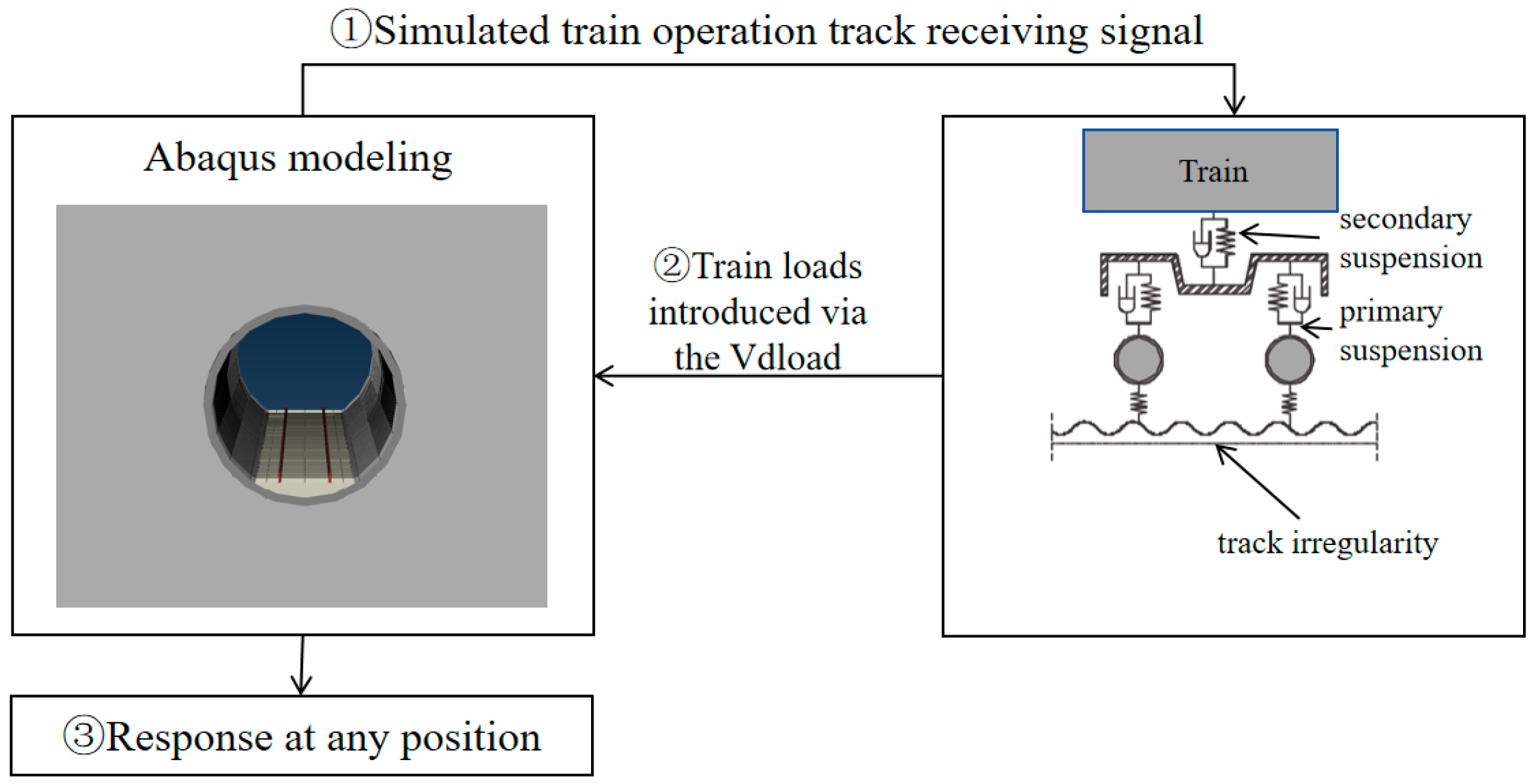
In Figure 1, we show the schematic for the analytical–numerical model. In this paper, a type-B subway train [24] is taken as the object of study. We use the vehicle–track coupled dynamic model which relies on a semi-analytical model and numerical simulation. By discretizing the equations of motion for the vehicle–track system and then solving them iteratively with a simple explicit integration method, we can obtain the forces at different times when the train is in contact with its rails, so we can quickly figure out how the whole system moves as it changes over time. When performing the calculations, a track irregularity spectrum is used for excitation input so that the actual operating condition of the track can also be represented. Then, we use the Vdload subroutine in Abaqus(2016) to apply the computed wheel–rail interaction forces during train operation to the Abaqus FEM model. In this way, we can obtain a mixture of two things, namely, vehicle–track dynamic analysis and finite element simulation; the first provides proper wheel–rail dynamic loadings, which are then analyzed by the finite element model to determine how vibrations propagate inside the tunnel as well as in the surrounding ground.

2.1. Subway Vehicle–Track Model

The dynamic governing equation of a subway train can be expressed as:

$$M\ddot{u}(t)+C\dot{u}(t)+Ku(t)=f(t)$$

(1)

where $M$, $C$, $K$ are the mass matrix, damping matrix and stiffness matrix of the structure; $\ddot{u}(t)$, $\dot{u}(t)$, $u(t)$ are the displacement, velocity, acceleration responses of the structure at any given time; $f(t)$ represents the time-varying external excitations applied to the structure.

In order to acquire the structural responses at every time step as well as increase the accuracy of computation, Newmark-β has been used for updating the response quantities so that both the accuracy of calculation and the stability of time integration can be improved:

$$\dot{u}(t+\Delta t)=\dot{u}(t)+[(1-\gamma )\ddot{u}(t)+\gamma \ddot{u}(t+\Delta t)]\Delta t$$

(2)

$$u(t+\Delta t)=u(t)+\dot{u}(t)\Delta t+[({\displaystyle \frac{1}{2}}-\beta )+\beta \ddot{u}(t+\Delta t)]\Delta t^2$$

(3)

where β and γ are the Newmark-β integration parameters which we take to be equal to 0.25 and 0.5 respectively here; Δt is the time step.

Equation (3) is equal to the following equation

$$u(t+\Delta t)=u(t)+\dot{u}(t)\Delta t+[({\displaystyle \frac{1}{2}}-\beta )+\beta \ddot{u}(t+\Delta t)]\Delta t^2$$

(4)

By combining Equations (2) and (4), the following expression can be obtained:

$$\dot{u}\left(t+\Delta t\right)={\displaystyle \frac{\gamma }{\beta \Delta t}}\left[u(t+\Delta t)-u(t)\right]+\left(1-{\displaystyle \frac{\gamma }{\beta }}\right)\dot{u}(t)+\Delta t\left(1-{\displaystyle \frac{\gamma }{2\beta }}\right)\ddot{u}(t)$$

(5)

Substitute Equations (3)–(5) into Equation (1), then we have:

$$\begin{gathered} \widehat{K}u\left(t+\Delta t\right)=\widehat{f}\left(t+\Delta t\right) \\ \widehat{K}=K+a_{0}M+a_{1}C \\ \widehat{f}\left(t+\Delta t\right)=f\left(t+\Delta t\right)+M\left(a_{0}u\left(t\right)+a_2\dot{u}(t)+a_3\ddot{u}(t)\right)+C\left(a_{1}u\left(t\right)+a_4\dot{u}(t)+a_5\ddot{u}(t)\right) \end{gathered}$$

(6)

where $a_0={\displaystyle \frac{1}{\beta \Delta t^2}}$, $a_1={\displaystyle \frac{\gamma }{\beta \Delta t}}$, $a_2={\displaystyle \frac{1}{\beta \Delta t}}$, $a_3={\displaystyle \frac{1}{2\beta }}-1$, $a_4={\displaystyle \frac{\gamma }{\beta }}-1$, $a_5=\Delta t\left({\displaystyle \frac{\gamma }{2\beta }}-1\right)$.

From Equations (2) and (4), we have the following for velocity and acceleration at our next time step:

$$\dot{u}(t+\Delta t)=\dot{u}(t)+a_6\ddot{u}(t)+a_7\ddot{u}(t+\Delta t)$$

(7)

$$\ddot{u}(t+\Delta t)=a_0[u(t+\Delta t)-u(t)]-a_2\dot{u}(t)-a_3\ddot{u}(t)$$

(8)

where $a_6=1-\gamma \Delta t$, $a_7=\gamma \Delta t$.

It is supposed that the vertical force of a wheel onto the rail is proportional to their difference in position:

$$F_z=K_{cr}\left(z_r-z_c+{\theta }_c{d}_d\right)$$

(9)

where K_cr is the vertical wheel–rail contact stiffness, z_r is the vertical displacement of the rail at the contact point, z_c is the vertical displacement of the wheelset, θ_c is the rotation angle of the wheelset about its transverse axis, and d_d is the vertical eccentric distance between the centroid of the wheelset and the contact point.

The displacement of the rail at the contact point can be evaluated by means of the Hermite shape functions for the beam element. Considering the vertical displacements and rotational angles at the two nodes of the element, it can be expressed as:

$$z_r(x)=N_1(x)w_1+N_2(x){\theta }_1+N_3(x)w_2+N_4(x){\theta }_2$$

(10)

where w₁, w₂ are the vertical displacements at each end node of element respectively, θ₁, θ₂ are the rotation angles at both ends of the element respectively, N₁(x)–N₄(x) are the Hermite interpolation functions, and x denotes the nodal position relative to the vehicle’s location.

The displacement at the rail contact point, z_r, is made up by the structural response displacement and the track irregularity displacement.

$$z_r(t)=z_r^{\mathrm{struct}}(t)+z_r^{\mathrm{irreg}}(t)$$

(11)

where z_r^struct(t) denotes the rail’s vertical displacement caused by the structural dynamic response, whereas z_r^irreg(t) denotes the additional displacement introduced by track irregularities.

For the numerical implementation, z_r^irreg(t) is added back in by adding it to the displacement at the contact point. Vertical track irregularity is most often expressed by its power spectral density. The spectrum adopted in this paper is from the American association of railroads (AAR), which can cover all the important wavelengths that control the dynamic responses of the metro vehicle–track system [25]. The concrete parameters of the AAR track spectrum can be seen in

Table 1. Parameters of AAR track spectrum [25].

Parameter	Track Class
	Class 1	Class 2	Class 3	Class 4	Class 5	Class 6
Av/(cm2·rad/m)	1.2107	1.0181	0.6816	0.5376	0.2095	0.0339
Ωc/(rad/m)	0.8245	0.8245	0.8245	0.8245	0.8245	0.8245

.

$$S(\Omega )={\displaystyle \frac{K_{\mathrm{c}}{A}_v{\Omega }_c^2}{{\Omega }^2({\Omega }^2+{\Omega }_c^2)}}$$

(12)

where Ω is the spatial angular frequency, K_c is the empirical correction coefficient, A_v is the power spectral density amplitude coefficient, and Ω_c is the cut-off angular frequency. The particular parameters for the AAR track spectrum are given in Table 1.

After getting the vertical contact force, it can be transformed into the right-hand-side vector of the vehicle equation F_c(t) and applied to finite element track model in the form of the equivalent nodal forces. This in turn forms the right-hand-side vector of the track equation, denoted by F_r(t).

The coupled dynamic equation of the vehicle is expressed as:

$$M_c{\ddot{u}}_c(t)+C_c{\dot{u}}_c(t)+K_c{u}_{\mathrm{c}}(t)=F_{grav}(t)+F_c(t)$$

(13)

The coupled dynamic equation of the track is expressed as:

$$M_r{\ddot{u}}_r(t)+C_r{\dot{u}}_r(t)+K_r{u}_r(t)=F_r(t)$$

(14)

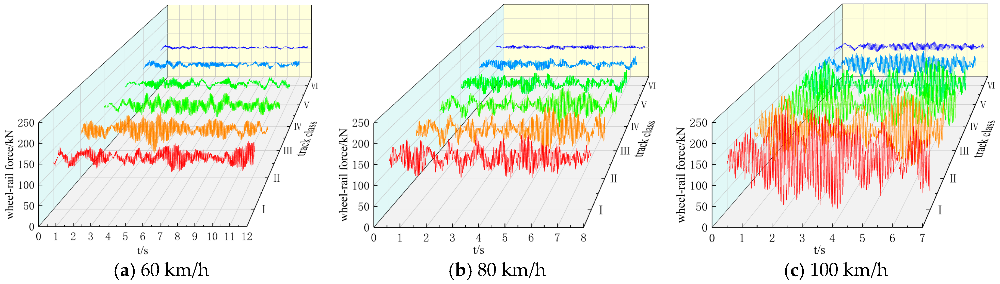
Figure 2 shows the time histories of wheel–rail interaction force at different track quality levels and train speeds. From Figure 2, we can see that at the same train speed, the greater the track irregularity, the larger the amplitude of the wheel–rail force. On the other hand, for the same track quality, as train speed rises, the amplitude of the wheel–rail force also increases.

2.2. Finite Element Modeling

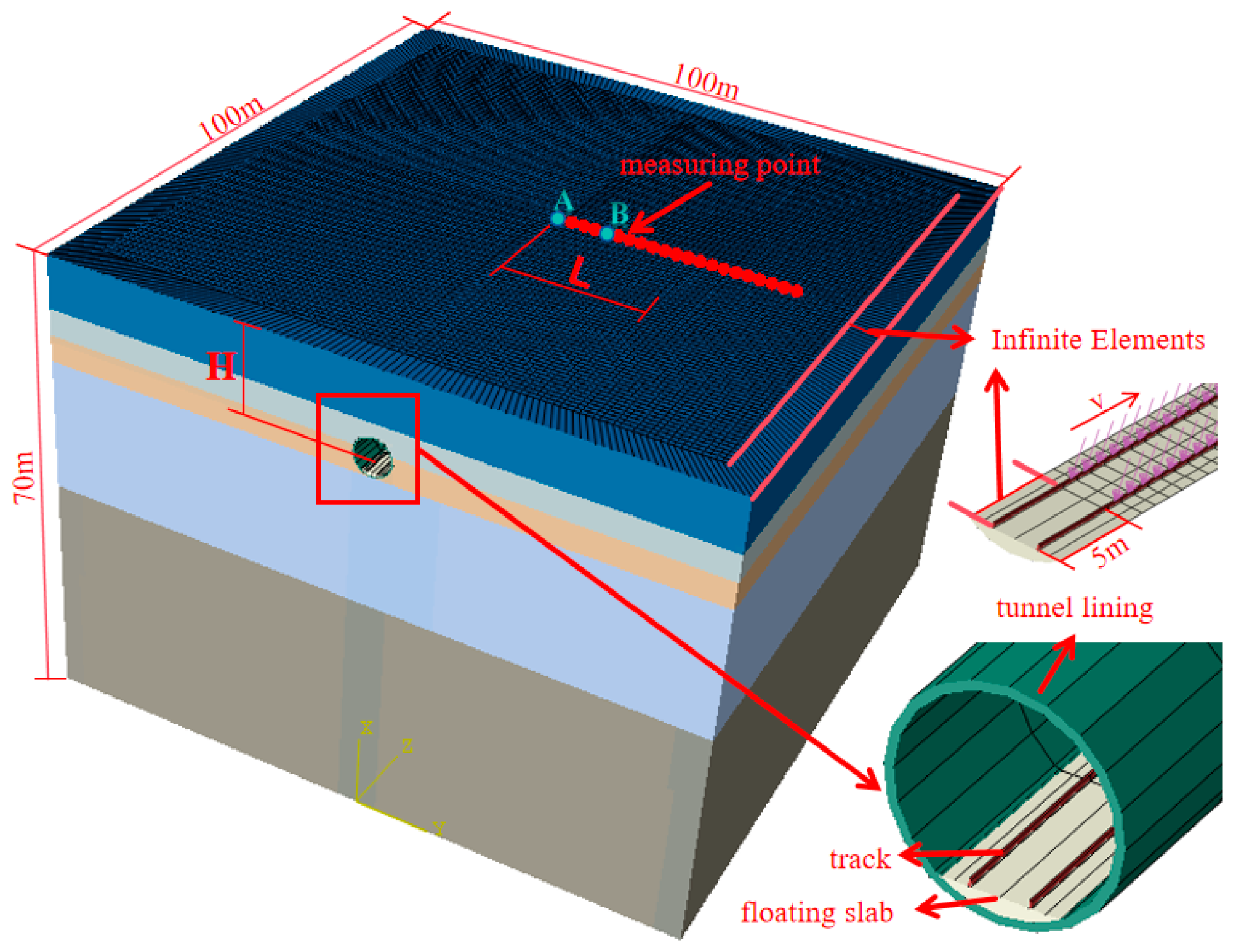
Figure 3 shows the finite element model of the track–tunnel–ground system set up in Abaqus. Soil domain dimensions are 100 m × 100 m × 70 m The tunnel’s inner diameter is set to be 2.7 m and the outer diameter has a value of 3.0 m, while the tunnel’s burial depth shall be referred to as H. For the sake of analyzing the change in vibration on the ground surface, some measuring points are set up on the model surface within transverse range L above the tunnel. In order to avoid spurious wave reflection at the model boundary, an artificial boundary is set up for the outer boundary of the model and the thickness of infinite element layer is taken as 5 m. Dynamic wheel–rail forces are applied from the point where the finite element region and infinite element region meet.

Type-B metro vehicles, grounds and tunnels calculation parameter lists can be found on

Table 2. Parameters of metro type-B vehicle.

Vehicle Parameters	Value	Unit
car body mass	39,540	kg
bogie mass	3520	kg
wheelset mass	1539	kg
roll moment of inertia of car body	32.4 × 103	kg·m2
pitch moment of inertia of car body	1328 × 103	kg·m2
yaw moment of inertia of car body	1317 × 103	kg·m2
roll moment of inertia of bogie frame	1430	kg·m2
pitch moment of inertia of bogie frame	1760	kg·m2
yaw moment of inertia of bogie frame	2950	kg·m2
roll moment of inertia of wheelset	1539	kg·m2
pitch moment of inertia of wheelset	104	kg·m2
yaw moment of inertia of wheelset	814	kg·m2
fixed wheelbase	2.2	m
longitudinal stiffness of primary suspension	10.6 × 103	kN/m
lateral stiffness of primary suspension	7.8 × 103	kN/m
vertical stiffness of primary suspension	1.7 × 103	kN/m
longitudinal stiffness of secondary suspension	0.21 × 103	kN/m
lateral stiffness of secondary suspension	0.21 × 103	kN/m
vertical stiffness of secondary suspension	0.45 × 103	kN/m
vertical damping of primary suspension	10	kN·s/m
vertical damping of secondary suspension	60	kN·s/m
lateral damping of secondary suspension	30	kN·s/m

,

Table 3. Geotechnical parameters.

Stratification/m	Density ρ /(kg/m3)	Elastic Modulus E /MPa	Poisson’s Ratio v	ξ
0–8	1600	168	0.35	0.02
8–12	1800	207	0.37	0.02
12–16	1900	388	0.3	0.02
16–36	2000	592	0.37	0.02
<36	2100	828	0.3	0.02

and

Table 4. Tunnel parameters.

Component Name	Density ρ /(kg/m3)	Elastic Modulus E /MPa	Poisson’s Ratio v
lining	2500	31,500	0.18
base	2500	28,000	0.2
rail	7830	210,000	0.3

[24]. As can be seen from Table 3, ξ is the Rayleigh damping ratio and can be obtained by Ref. [26].

2.3. Convergence Analysis

Recommendations for the mesh size and time-step selection in finite element modeling have been given in Refs. [27,28]. The maximum mesh size should satisfy ${\Delta }_x<C_s/(6f_{\max })$, where Δ_x is the finite element size, C_s is the shear wave velocity of the soil layer where the tunnel is located, and f_max is the maximum frequency considered in the analysis. The time step is determined by $\Delta t\le {\Delta }_x\sqrt{\rho /E}$, where ρ is the material density and E is the elastic modulus. The maximum frequency of the AAR track spectrum adopted in this study is 40 Hz, and the shear wave velocity of the soil layer in which the tunnel is located is 261 m/s. In addition, the maximum mesh sizes of the soil and track in the model are 1 m and 0.5 m, respectively, and the time step is 0.001 s, which satisfies the recommendations given in Refs. [27,28].

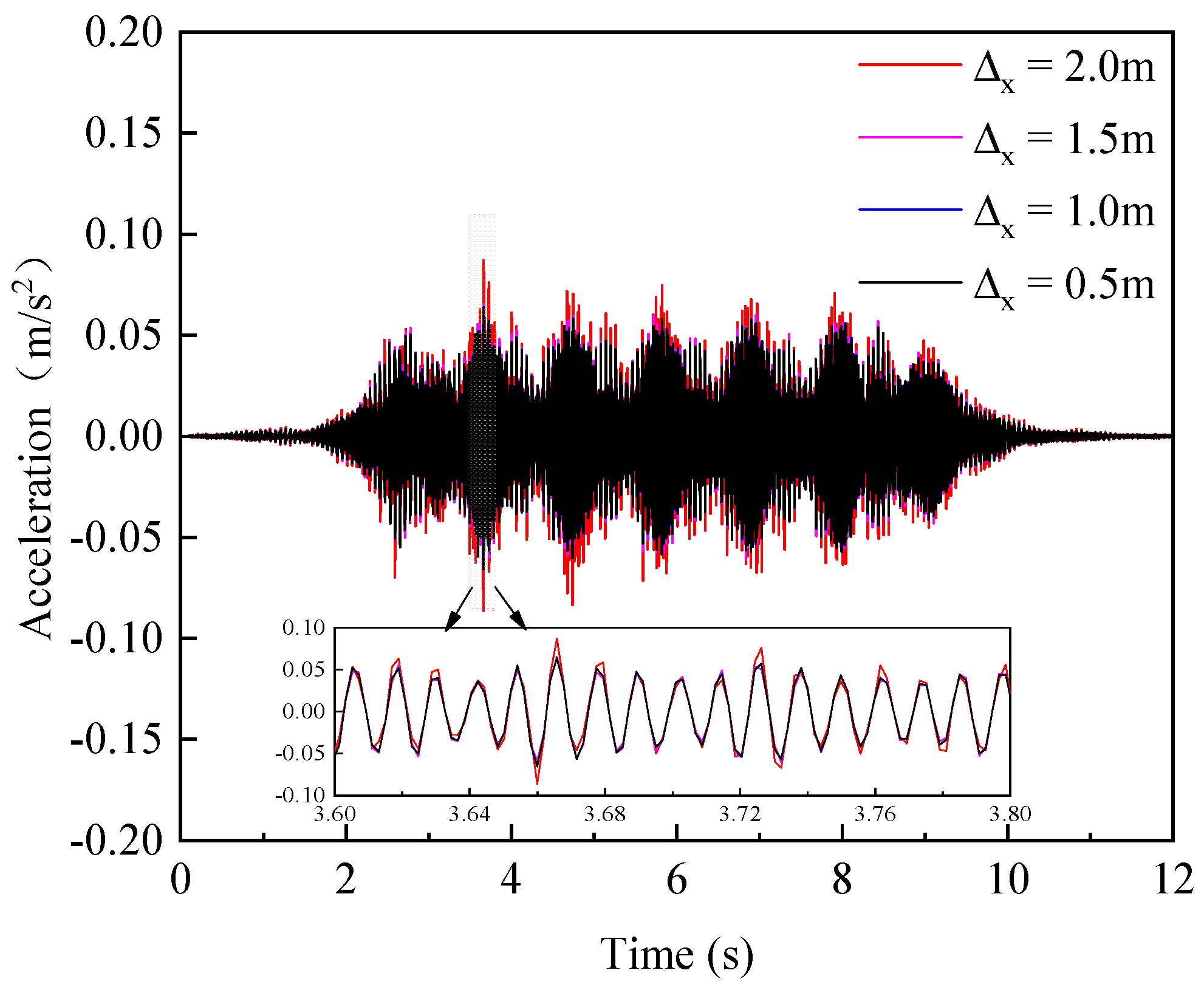
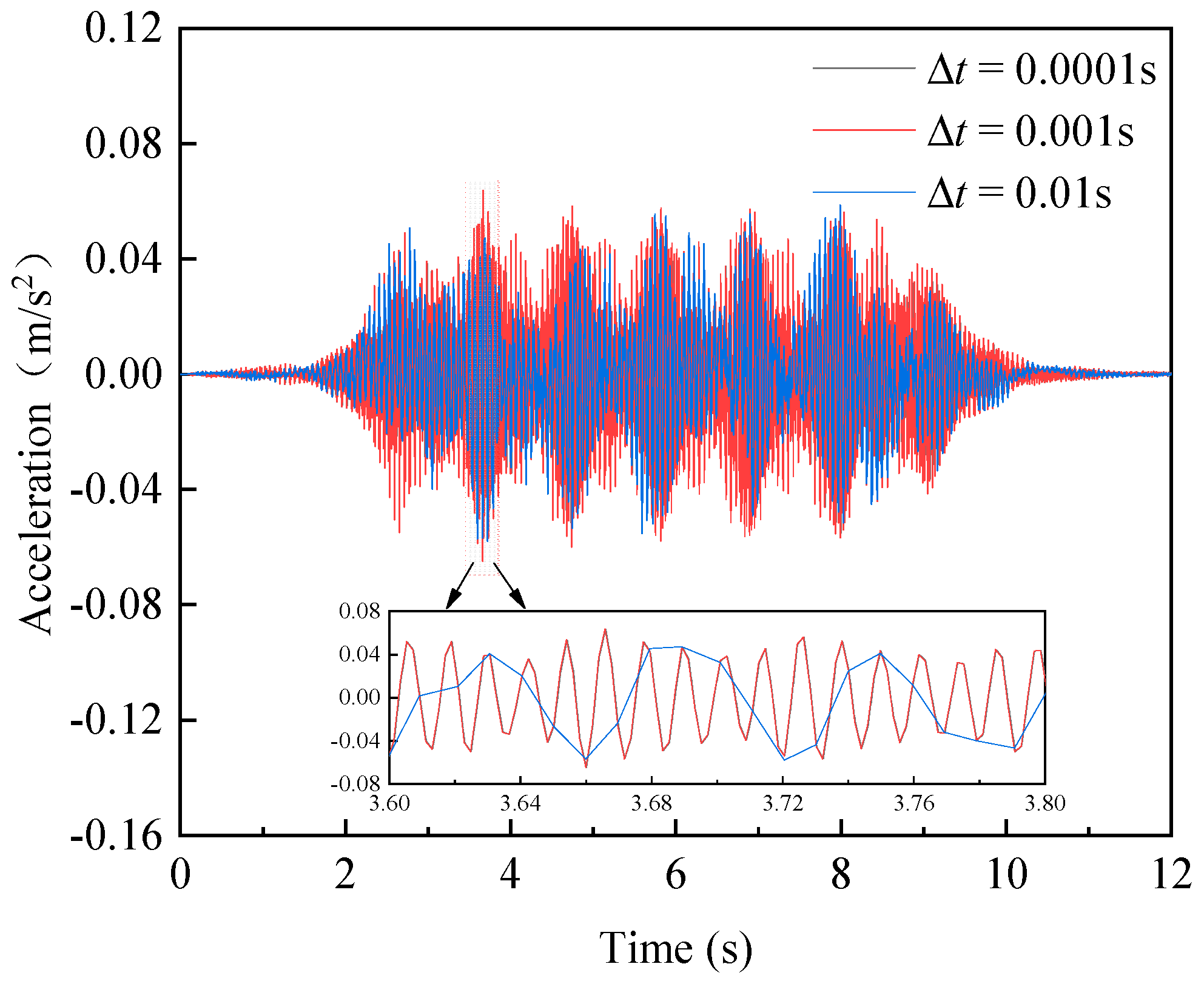
Take the train speed to be 60 km/h, take the track state to be Class 6 irregularity. As can be seen from Figure 4, the acceleration time-history curve at point A (see Figure 3) with different meshing. From Figure 4 we see that when the mesh is decreased from 1.5 m to 1 m there is only a minor change in acceleration, and when it goes from 1 m down to 0.5 m the response is basically no different. It means when the value of mesh size reaches 1 m, then it has converged. Figure 5 is the acceleration time-history curves of point A with different time steps. When the time step is changed from 0.001 s to 0.0001 s, we can see that there is almost no change in the acceleration response; therefore, it has been proven that when the time step was set at 0.001 s, the numerical results were stable. Considering the calculation speed of the model, the mesh is 1 m, and the time step is set to 0.001 s.

3. Model Validation

To test whether the calculation method is right or not, we calculate the wheel–rail force at first.

Table 5. Comparison of wheel–rail force amplitudes and mean values.

v /(km/h)	80			70			60			50
	Ref. [29]	This Paper	Error%	Ref. [29]	This Paper	Error%	Ref. [29]	This Paper	Error%	Ref. [29]	This Paper	Error%
max	75,827	75,324	0.66	73,574	72,613	1.30	71,615	71,009	0.85	70,295	67,756	3.61
min	52,296	53,609	2.51	55,846	56,830	1.76	56,501	58,022	2.69	60,164	60,191	0.05
mean	64,667	64,565	0.16	64,660	64,560	0.15	64,672	64,518	0.24	64,672	64,601	0.11

compares the results obtained from this work and Ref. [29]. It can be seen that the maximal deviation between the two sets of results is 3.61%, and the mean relative error (RE) is 1.17%. This difference is because the analytical model and numerical model are coupled in a one-way manner, so it does not consider the feedback from tunnel–ground response to the vehicle dynamic. But it is very small in practical engineering. Therefore, the proposed calculation method can reasonably reflect the dynamic characteristics of wheel–rail interaction under train operation.

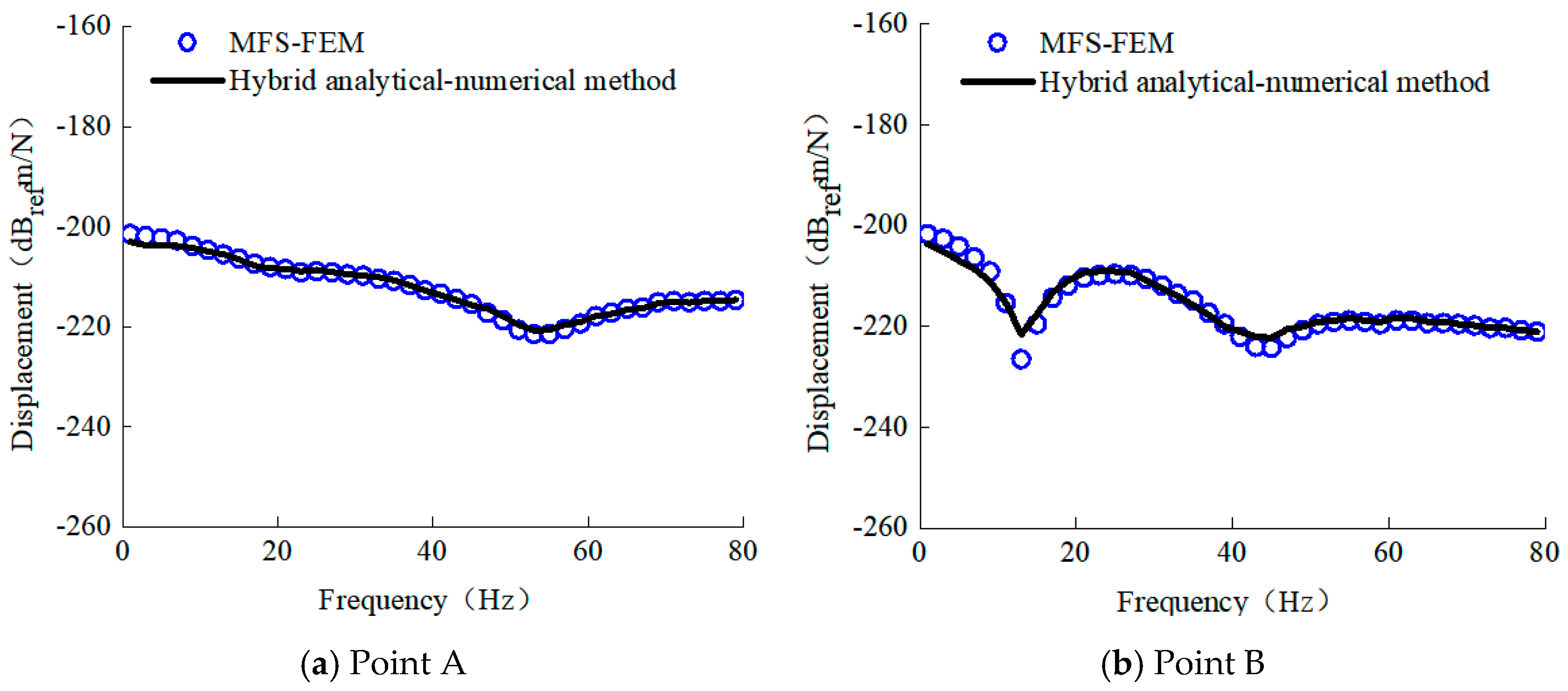
In order to prove that our model is correct, we set up a finite element in Abaqus. It is supposed that the ground is a single type of soil layer, with the shear wave velocity being 250 m/s; the compressional wave velocity is 468 m/s, the density is 1900 kg/m³ and the damping ratio is 0.04. Tunnel structure takes the form of round sections, model parameters are: tunnel center point H equal to 9 m, the wall thickness e = 0.3 m for a tunnel lining, E equals 30 GPa, v is set to be 0.15, ρ taking on the value of 2500 kg/m³. The displacement spectra of the monitoring point A and the monitoring point B (see Figure 3) are calculated and the result is compared with the calculation results by the MFS–FEM hybrid method [30], as shown in Figure 6. From Figure 6 we can see that the calculation result in this study agrees with the results reported by reference [30] well, so it shows the validity and reliability of the calculated method in this research.

To assess the accuracy of the proposed model, a finite element model was developed in Abaqus. The ground was idealized as a homogeneous soil medium, with a shear wave velocity of C_s = 250 m/s, a compressional wave velocity of C_p = 468 m/s, a density of ρ = 1900 kg/m³, and a damping ratio of ξ = 0.04. The tunnel was simplified as a circular cross-section, and its main parameters included a burial depth of H = 9 m, a lining thickness of e = 0.30 m, an elastic modulus of E = 30 GPa, a Poisson’s ratio of v = 0.15, and a lining density of ρ = 2500 kg/m³. The displacement spectra at monitoring point A and point B (Figure 3) were then calculated and compared with the results of the MFS–FEM hybrid approach reported in Ref. [30], as shown in Figure 6. The comparison shows that the present results are in good agreement with those in Ref. [30], indicating that the proposed method can provide reliable predictions.

4. Numerical Example Analysis

To study the ground surface response induced by train loading in the tunnel, we have taken the value of H = 13 m. Monitoring points were laid on different places from the tunnel centerline, with a spacing of 2 m, extending to around 1.5 H away from the tunnel centerline, as shown in Figure 3.

4.1. Influence of Track Irregularities on Ground Surface Vibrations

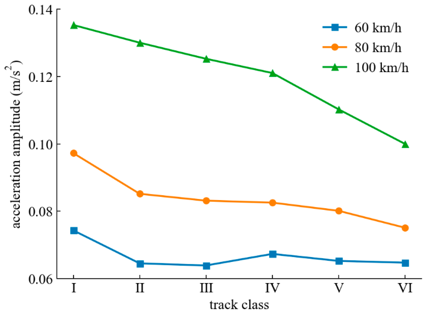
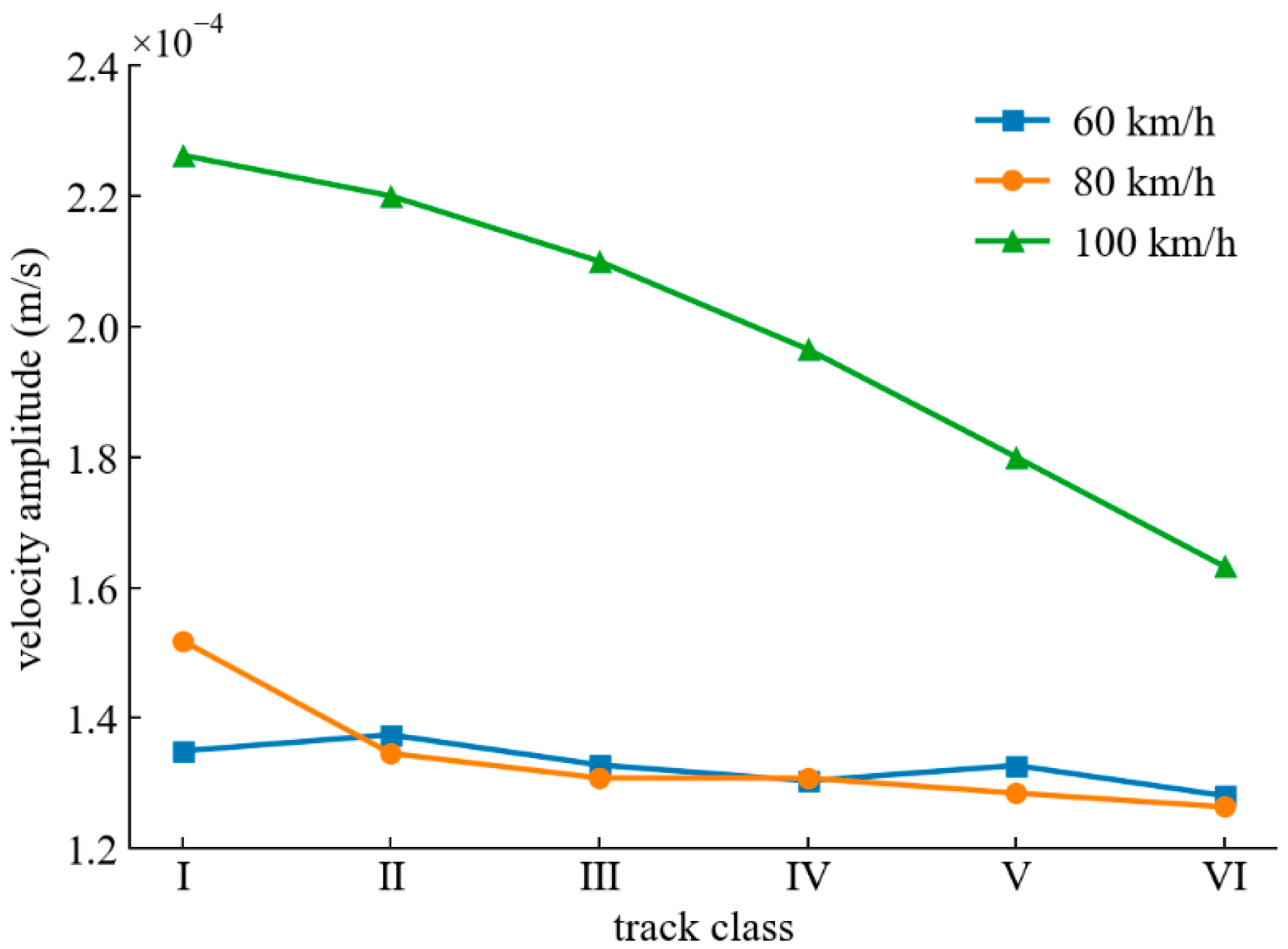
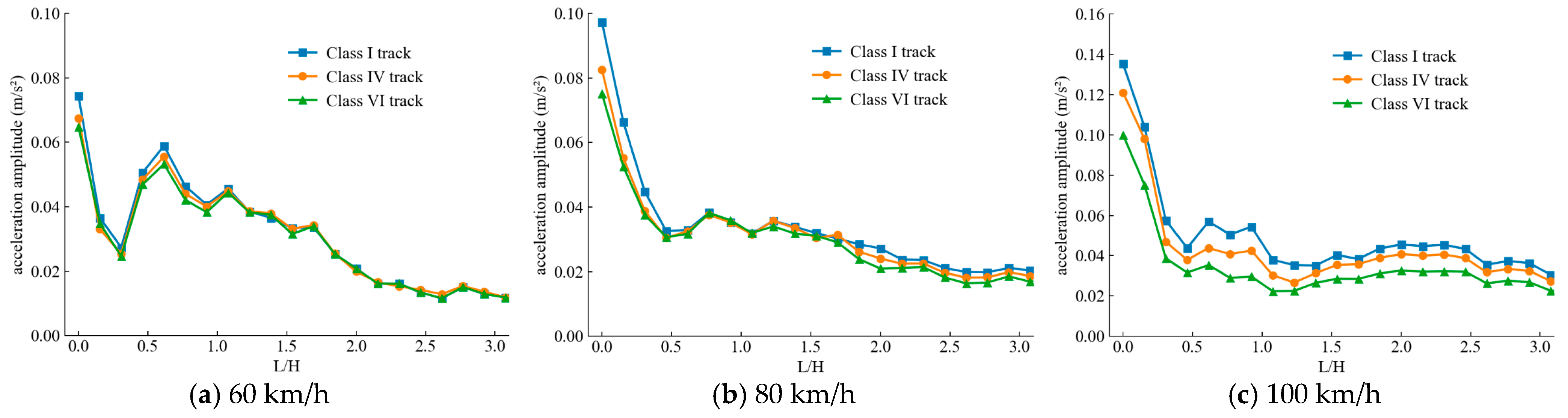
Figure 7 and Figure 8 show the variations in the amplitude of ground surface acceleration and the amplitude of ground surface velocity at the center of the ground surface under different track quality levels and train operating speeds. From Figure 7 and Figure 8, we can see that with the increase in train speed, the amplitude of ground surface acceleration and velocity increases. As a result of the train going faster, the frequency and intensity of force vibrations produced by the wheel–rail contact increase, so more energy is transferred from the train to the ground. The amplitude of the ground surface vibration under the same train speed will be smaller with the improvement of the track quality level (i.e., the better the track is). For the ground surface acceleration amplitude when a high-speed train runs, it is even more prominent. Thus, the level of ground surface vibration is jointly regulated by the train’s operating speed and the track’s quality level. The speed of the train decides the general strength of the vibration. It regulates the vibration response via the smoothness of the track.

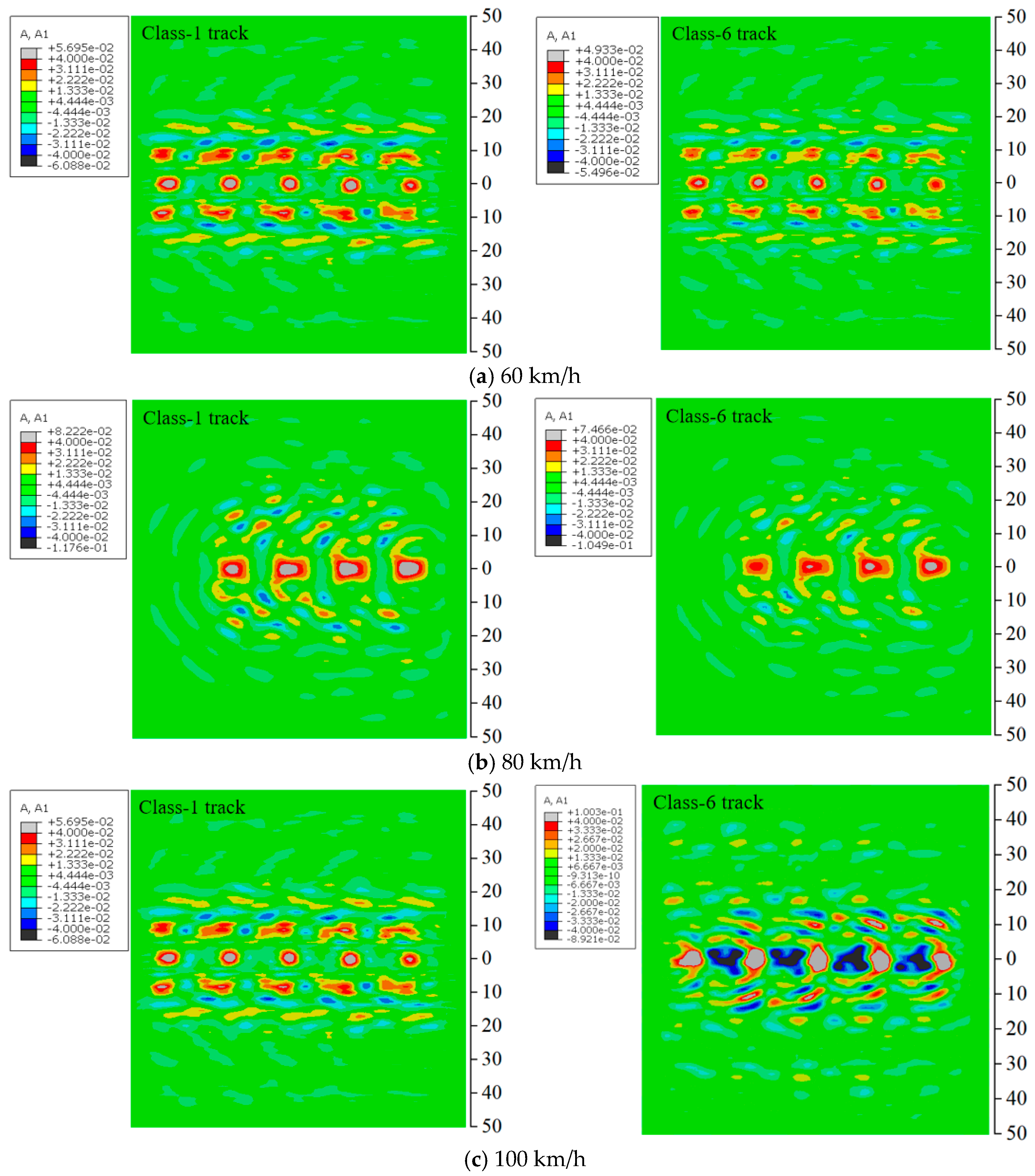
From Figure 9 we can see the spatial distribution contour of ground surface acceleration amplitude when the train is running. As can be seen from Figure 9, the acceleration amplitude above the tunnel is greatly amplified; there is also an amplification area on both sides of the tunnel. (The amplification area is defined as a certain area where the impact produced by rail transit operation on the ground does not decrease at all with the increase in distance from the railway track. On the contrary, within a specific range around the tunnel centerline, the vibration amplitude is remarkably high, creating an abnormal peak zone of vibration.) When the train speed is 60 km/h, there will be an amplification phenomenon in the area extending about 17 m centered on both sides of the tunnel centerline: when the train running speed is 80 km/h, the amplification region is about 25 m on both sides of the tunnel center line. As the speed of the train rises more, it could extend out to around 40 m from the center line of the tunnel on either side. It means that the higher the train speed, the farther the ground surface vibration can propagate. Also, as can be seen from Figure 9, when the same train operating speed is considered for different track quality levels, the smaller amplification region is accompanied by smaller acceleration amplitudes which become larger as the operating speed increases.

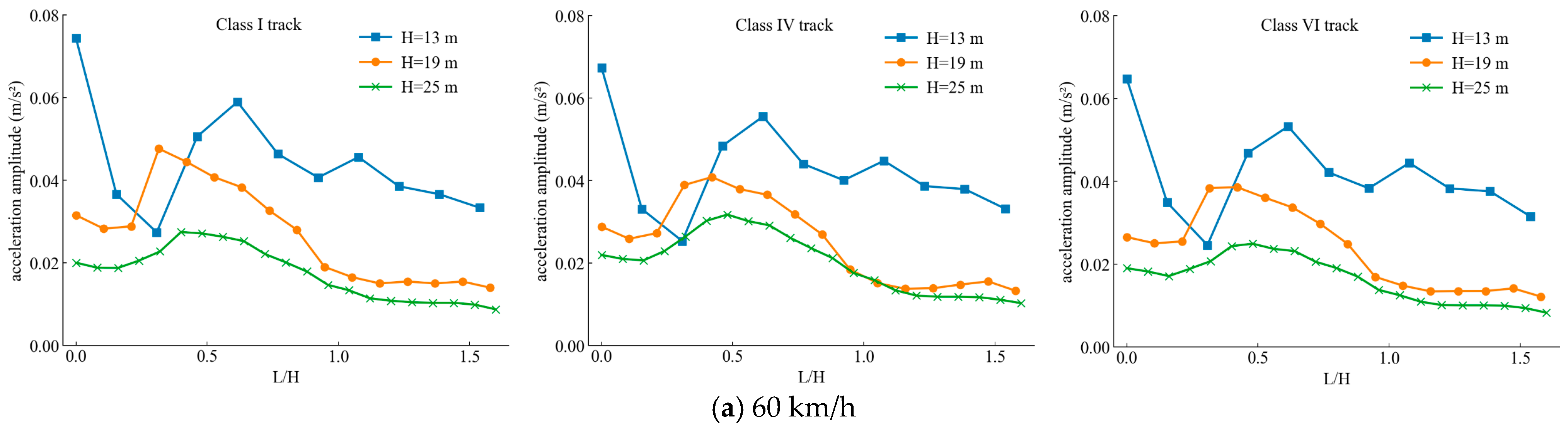
Figure 10 gives the variation curves of acceleration peak at the ground surface observation point (see Figure 3) The acceleration peak is at its highest value immediately above the center of the tunnel and rapidly decays after about 0.4 H from the tunnel crown. Within 0.4 H–1.4 H of the tunnel centerline there are some local amplification zones. After more than 1.4 H the acceleration amplitude becomes stable; in general it is less than 0.04 m/s² which means the vibration level on the ground is low: the impact of the track quality grade is very important in terms of acceleration amplitude at 1.4 H above the tunnel. In the case of high-speed train running, the decrease in vibration magnitude is obvious after increasing the track grade. The train running speed also decides how much overall energy is contained in the vibration. When the train runs slowly (60 km/h), it is easy for the amplitude in the amplification region to stand out. But at 80 km/h and 100 km/h, the difference in amplitudes among all parts in the amplification area becomes less noticeable. The track’s quality level mainly has a controlling effect; the better the track quality, the smaller the amplitude of the acceleration on the ground.

4.2. Analysis of Ground Surface Vibration Responses Under Different Tunnel Burial Depths

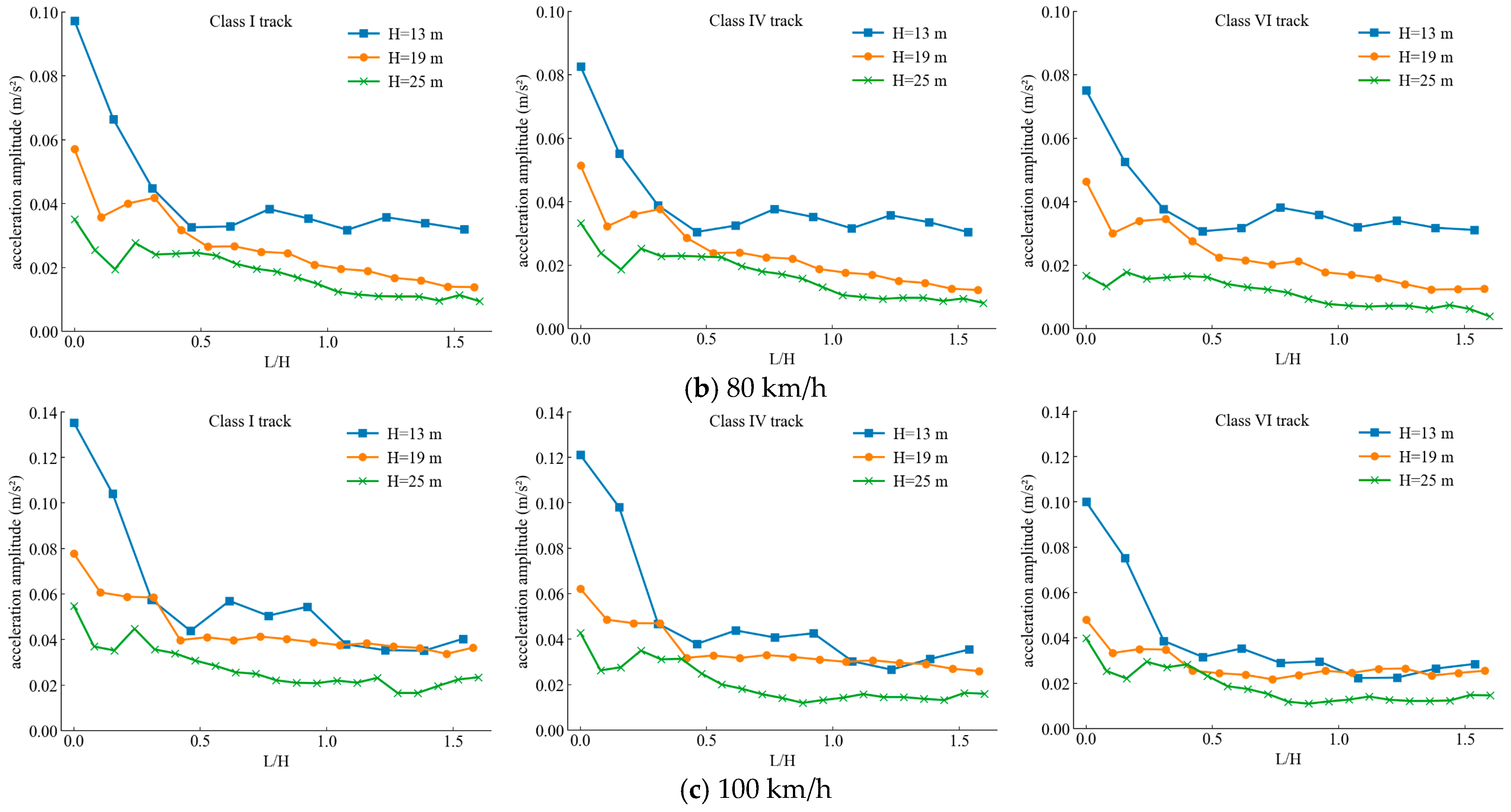
Figure 11 shows a comparison of the ground surface acceleration amplitudes under different tunnel burial depths. As can be seen from Figure 11, as the tunnel burial depth increases, the acceleration amplitudes directly above the tunnel decrease significantly, and the amplification zones on both sides also tend to move closer to the tunnel centerline. On the basis of the same train operating speed, the spatial distribution characteristics of the acceleration amplitude influenced by burial depth have a similar change law for different track qualities. Also with respect to the same track quality level, the higher the train speed is, the more remarkable the attenuation influence of increased tunnel burial depths on ground surface acceleration amplitude will become. So, we can control the vibration caused by the running of subway through the speed and reasonable deepening of the tunnel.

5. Conclusions

Using the analytical–numerical hybrid approach, a coupled dynamic model of the vehicle–track–tunnel–ground system was developed. The effects of track quality level, train speed, and tunnel burial depth on ground surface vibration propagation were then examined in a systematic manner. The main findings are summarized as follows:

(1) Make up a metro vibration prediction analytical–numerical jumble method: when the analytical vehicle–tracks dynamic model is linked with the numerical tunnels–ground system model, it allows us to bring in much more realistic time varying wheel–rail force and takes full account of the effects due to track irregularity. At the same time, we can have a finer modeling of the tunnel itself and the soil around it which makes this computation more efficient.

(2) Track quality and train operating speed jointly affect the ground surface vibration response. Improved track smoothness reduces the vibration level at the ground surface, and this tendency becomes more evident under high-speed conditions. In addition, an amplification zone is observed in the ground surface response within approximately 0.4–1.4 H from the tunnel centerline.

(3) Increasing the tunnel burial depth can significantly reduce the ground surface vibration level. As the burial depth increases, both the acceleration amplitude directly above the tunnel and the extent of the amplification zones on both sides decrease markedly.

In this paper, we propose a kind of analytic–numerical combined method which can be used to research the dynamic behaviors between vehicle, train, tunnel and ground. It provides a brand-new solution about how we should think of the vibration caused by the metro on the Earth’s surface. But, the effect of soil nonlinearity and porous multiphase nature and also the nonlinear effect of wheel–rail contact is still not considered for the vibration response. And the other factors and their effects on metro-induced vibration will be studied more.

References

1. Shao, Z.; Bai, W.; Dai, J.; Sun, G. Measurement and analysis of vibration responses due to subway transit in residential areas. Structures 2024, 69, 107305. [Google Scholar] [CrossRef]
2. He, Y.; Zhang, Y.; Yao, Y.; He, Y.; Sheng, X. Review on the Prediction and Control of Structural Vibration and Noise in Buildings Caused by Rail Transit. Buildings 2023, 13, 2310. [Google Scholar] [CrossRef]
3. Liang, Y.; Zhou, F.; Cao, X.; Wang, L.; Zhu, S.; Zhou, Z. Time-domain analysis for the scattering of plane elastic waves in half-space with an open trench. J. Vib. Control. 2022, 30, 354–365. [Google Scholar] [CrossRef]
4. Thompson, D.J.; Kouroussis, G.; Ntotsios, E. Modelling, simulation and evaluation of ground vibration caused by rail vehicles. Veh. Syst. Dyn. 2019, 57, 936–983. [Google Scholar] [CrossRef]
5. Sheng, X. A review on modelling ground vibrations generated by underground trains. Int. J. Rail Transp. 2019, 7, 241–261. [Google Scholar] [CrossRef]
6. Shang, X.; Guo, M.; Wang, G.; Zhao, J.; Pan, D. Behavioral model construction of architectural heritage for digital twin. Npj Herit. Sci. 2025, 13, 129. [Google Scholar] [CrossRef]
7. Sun, H.; Fang, Y.; Yuan, Z.; Weng, Z.; Ni, D. Analytical modeling for the calculation of underground train-induced vibrations in inhomogeneous soils with uncertainty. AIP Adv. 2021, 11, 115321. [Google Scholar] [CrossRef]
8. Karlström, A.; Boström, A. An analytical model for train-induced ground vibrations from railways. J. Sound Vib. 2006, 292, 221–241. [Google Scholar] [CrossRef]
9. Yuan, Z.; Cai, Y.; Sun, H.; Shi, L.; Pan, X. The influence of a neighboring tunnel on the critical velocity of a three-dimensional tunnel-soil system. Int. J. Solids Struct. 2021, 212, 23–45. [Google Scholar] [CrossRef]
10. Hussein, M.F.M.; Hunt, H.E.M. A numerical model for calculating vibration from a railway tunnel embedded in a full-space. J. Sound Vib. 2007, 305, 401–431. [Google Scholar] [CrossRef]
11. Triepaischajonsak, N.; Thompson, D. A hybrid modelling approach for predicting ground vibration from trains. J. Sound Vib. 2015, 335, 147–173. [Google Scholar] [CrossRef]
12. Yuan, Z.; Xu, D.; Shi, L.; Pan, X.; He, B.; Hu, M.; Cai, Y. Hybrid analytical-numerical modelling of ground vibrations induced by underground trains in saturated soil. Eur. J. Environ. Civ. Eng. 2022, 26, 6047–6075. [Google Scholar] [CrossRef]
13. Zhai, W.; Wang, K.; Cai, C. Fundamentals of vehicle–track coupled dynamics. Veh. Syst. Dyn. 2009, 47, 1349–1376. [Google Scholar] [CrossRef]
14. Zhai, W.; Stichel, S.; Ling, L. Train–track coupled dynamics problems in heavy-haul rail transportation. Veh. Syst. Dyn. 2025, 63, 1187–1240. [Google Scholar] [CrossRef]
15. Zhai, W.; Han, Z.; Chen, Z.; Ling, L.; Zhu, S. Train–track–bridge dynamic interaction: A state-of-the-art review. Veh. Syst. Dyn. 2019, 57, 984–1027. [Google Scholar] [CrossRef]
16. Fu, Q.; Zheng, C. Three-dimensional dynamic analyses of track-embankment-ground system subjected to high speed train loads. Sci. World J. 2014, 2014, 924592. [Google Scholar] [CrossRef]
17. Gao, G.; Zhang, J.; Chen, J.; Bi, J. Investigation of saturation effects on vibrations of nearly saturated ground due to moving train loads using 2.5D FEM. Soil Dyn. Earthq. Eng. 2022, 158, 107288. [Google Scholar] [CrossRef]
18. Hussein, M.; François, S.; Schevenels, M.; Hunt, H.; Talbot, J.; Degrande, G. The fictitious force method for efficient calculation of vibration from a tunnel embedded in a multi-layered half-space. J. Sound Vib. 2014, 333, 6996–7018. [Google Scholar] [CrossRef]
19. Gupta, S.; Degrande, G. Modelling of continuous and discontinuous floating slab tracks in a tunnel using a periodic approach. J. Sound Vib. 2010, 329, 1101–1125. [Google Scholar] [CrossRef]
20. Gupta, S.; Van den Berghe, H.; Lombaert, G.; Degrande, G. Numerical modelling of vibrations from a Thalys high speed train in the Groene Hart tunnel. Soil Dyn. Earthq. Eng. 2010, 30, 82–97. [Google Scholar] [CrossRef]
21. Jin, Q.; Thompson, D.J.; Lurcock, D.E.; Toward, M.G.; Ntotsios, E. A 2.5D finite element and boundary element model for the ground vibration from trains in tunnels and validation using measurement data. J. Sound Vib. 2018, 422, 373–389. [Google Scholar] [CrossRef]
22. Ghangale, D.; Arcos, R.; Clot, A.; Cayero, J.; Romeu, J. A methodology based on 2.5D FEM-BEM for the evaluation of the vibration energy flow radiated by underground railway infrastructures. Tunn. Undergr. Space Technol. 2020, 101, 103392. [Google Scholar] [CrossRef]
23. Di, H.; Zhou, S.; Luo, Z.; He, C.; Xiao, J.; Li, X. A vehicle-track-tunnel-soil model for evaluating the dynamic response of a double-line metro tunnel in a poroelastic half-space. Comput. Geotech. 2018, 101, 245–263. [Google Scholar] [CrossRef]
24. Zheng, H.S. Study on the Vibration Impact of Metro Operation on Adjacent Buildings and the Effectiveness of Different Control Measures. Master’s Thesis, Beijing Jiaotong University, Beijing, China, 2024. [Google Scholar]
25. Zhai, W. Vehicle–Track Coupled Dynamics: Theory and Applications; Springer: Singapore, 2020. [Google Scholar]
26. Chowdhury, I.; Dasgupta, S. Computation of Rayleigh damping coefficients for large systems. Electron. J. Geotech. Eng. 2003, 43, 6855–6868. [Google Scholar]
27. Qiu, L.; Yan, X.X.; Lin, X.D.; Yuan, S.F. Multiphysics simulation method of Lamb wave propagation with piezoelectric transducers under load condition. Chin. J. Aeronaut. 2019, 32, 1071–1086. [Google Scholar] [CrossRef]
28. Dassault Systèmes Simulia Corp. Abaqus/Explicit Analysis: Stability and Time Incrementation [EB/OL]; Abaqus 2024 Documentation; Dassault Systèmes Simulia Corp: Providence, RI, USA, 2024. [Google Scholar]
29. Zhang, Q.L.; Liu, L.Y.; Li, J.Y. Prediction of dormitory environmental vibration induced by metro operation and study on vibration isolation measures. J. Disaster Prev. Mitig. Eng. 2015, 35, 745–751. [Google Scholar]
30. Amado-Mendes, P.; Alves Costa, P.; Godinho, L.M.C.; Lopes, P. 2.5D MFS–FEM model for the prediction of vibrations due to underground railway traffic. Eng. Struct. 2015, 104, 141–154. [Google Scholar] [CrossRef]
Figure 1. Schematic diagram of the hybrid analytical–numerical model.
Applsci 16 04668 g001
Figure 2. Wheel–rail force time histories under different speeds.
Applsci 16 04668 g002
Figure 3. Schematic diagram of the Abaqus model.
Applsci 16 04668 g003
Figure 4. Acceleration time-history curves at monitoring point A under different mesh sizes.
Applsci 16 04668 g004
Figure 5. Acceleration time-history curves at monitoring point A under different time steps.
Applsci 16 04668 g005
Figure 6. Comparison between the analytical–numerical hybrid method and the MFS–FEM hybrid method.
Applsci 16 04668 g006
Figure 7. Comparison of ground surface central acceleration amplitudes under different track classes.
Applsci 16 04668 g007
Figure 8. Ground surface central velocity amplitude comparison of different rail ways classes.
Applsci 16 04668 g008
Figure 9. Ground vertical acceleration contour plots.
Applsci 16 04668 g009
Figure 10. Comparison of ground acceleration amplitudes under different track classes.
Applsci 16 04668 g010
Figure 11. Comparison of the amplitude of ground acceleration at various burial depths.
Applsci 16 04668 g011aApplsci 16 04668 g011b