Game-Theoretic Design Optimization of Switched Reluctance Motors for Air Compressors to Reduce Electromagnetic Vibration

Abstract

Switched reluctance motors (SRMs) are promising for applications such as air compressors due to their robust structure and fault tolerance, but suffer from high torque ripple and radial electromagnetic forces that cause vibration and noise. This paper proposes a game-theoretic multi-objective design optimization framework to enhance electromagnetic performance by simultaneously maximizing average torque and minimizing radial force. The optimization problem is transformed into a game model where objectives are treated as players with strategy spaces derived through fuzzy clustering and correlation analysis. Particle swarm optimization (PSO) is employed to solve the payoff functions under both novel cooperative and non-cooperative game scenarios of SRMs’ structural design. Finite element analysis (FEA) validates the optimized motor topology, showing that the cooperative game model achieves a balanced performance with high torque density and reduced vibration, meeting the requirements for air compressor drives. The proposed method effectively resolves the weight selection challenge in traditional multi-objective optimization and demonstrates strong engineering feasibility.

1. Introduction

Switched reluctance motors (SRMs) are widely applied in electric vehicles, the aerospace industry, and industrial drives due to their simple and robust construction, low cost, and excellent fault tolerance capability [1,2]. However, their double salient pole structure and pulsed excitation method generate significant torque ripple and radial electromagnetic forces, which subsequently induce vibration and acoustic noise issues [3]. These limitations restrict the application of SRMs in important technologies, such as air compressors and high-precision servo positioning systems. Currently, one of the most common approaches to addressing the inherent limitations of switched reluctance motors is to optimize electromagnetic performance by improving their design, aiming to maximize the average electromagnetic torque while minimizing radial electromagnetic forces [4,5,6,7].

Electromagnetic performance optimization of switched reluctance motors (SRMs) involves multiple variables, strong nonlinearity, and complex mathematical models while maintaining compliance with specific constraints to achieve globally balanced performance metrics such as efficiency, torque, power density, and vibration. Current research predominantly employs intelligent algorithms (e.g., genetic algorithms, particle swarm optimization) for multi-objective optimization of motor structural parameters.

In [8], the authors addressed multi-objective optimization regarding efficiency and torque ripple in motor design using a Genetic–Fuzzy Algorithm (GFA), significantly improving computational efficiency through a fuzzy expert system. Experimental results demonstrated that this method not only enhanced motor efficiency (92.7% → 93.1%) and reduced torque ripple (28.44% → 10.4%) but also achieved a 17.1% reduction in motor weight. However, the expert system constructed from fuzzy rules relies on the initial dataset. If the design parameter range is expanded, the rule base requires retraining. Additionally, the fuzzy weights in the multi-objective function require manual intervention.

The authors of [9] proposed a multi-objective optimization approach integrating fuzzy inference with NSGA-III. This method employs a Mamdani system to quantify designer preferences by generating relative weight values, which subsequently guide the algorithm to search preferred regions. Their approach effectively addresses the ranking challenges of Pareto solutions in switched reluctance generator design optimization. Case studies demonstrate that the proposed method significantly outperforms conventional NSGA-III in key metrics, including efficiency (+6.2%) and torque ripple reduction (−6.5%), while exhibiting superior decision-making efficiency. However, the computational complexity and substantial computational cost associated with the numerous finite element simulations required remain a challenge for practical industrial deployment, which will be addressed in future work.

Ma et al. proposed a multi-objective optimization framework for SRMs that integrates design of experiments (DoE) and particle swarm optimization (PSO) [10]. By using definitive screening design (DSD) to reduce variable dimensionality and by replacing finite element analysis (FEA) with a third-order response surface model, their approach reduced computational costs by 80% while maintaining accuracy. Experimental results demonstrated significant improvements in key performance metrics, including a 27.15% reduction in torque ripple and a 9.51% increase in torque per unit mass, with substantially higher Pareto frontier generation efficiency compared to conventional methods. The core contribution of their work lies in resolving the trade-off between precision and efficiency in high-dimensional electromechanical system optimization.

In [11], Afifi et al. employed a multi-objective genetic algorithm (MOGA) to optimize SRM performance, simultaneously considering multiple criteria, including average torque, efficiency, core weight, torque ripple, and temperature increase. Their study integrated FEA and dynamic simulation to accurately compute electromagnetic and thermal characteristics. The effectiveness of their optimized design was verified through efficiency maps and torque curves. Their simulation results demonstrated that the optimized solution meets the electric vehicle requirements for a high starting torque, wide high-efficiency regions, and low manufacturing costs, thereby providing a viable solution for SRM applications in electric transportation.

In [12], Zhang et al. proposed a fast and universal multi-objective design and optimization method for SRMs based on an analytical model and PSO algorithm. Their study established an analytical model applicable to arbitrary stator and rotor slot combinations and reduced the optimization variables to five key parameters. Using the PSO algorithm, their method can generate optimal design solutions that satisfy various performance criteria (e.g., torque, efficiency, weight, and volume) within minutes. Comparative studies with FEA results validated the method’s accuracy and computational efficiency. This approach overcomes the empirical dependence and time-consuming computations of traditional design methods, providing an efficient and flexible solution for SRM design.

These research outcomes demonstrate that multi-objective optimization is an effective approach to improving SRM structural design. Current efforts aim to enhance overall motor performance and reconcile conflicting design metrics through multi-objective optimization methodologies. In the studies reviewed, unified objective functions were typically formulated by weighted summation of multiple performance indicators, in which weight selection was critical. Notably, Reference [9] employed a Mamdani system to quantify designer preferences and generate relative weight values. Building upon the proven success of game theory in mechanical design domains [13,14,15,16], this work extends its application to electromagnetic optimization in electric machine design.

Miyamoto [17] addresses the design optimization of a surface permanent magnet motor with three conflicting objectives—namely, minimizing copper and iron loss and cogging torque—by integrating non-cooperative and cooperative game theory. Noguchi [18] proposes a commonality-based design method using game theory for a series of structurally similar surface permanent magnet motors of different sizes, achieving a balance between motor efficiency and economic efficiency. Both studies established a game-theoretic systematic framework for multi-objective motor design optimization, but they have certain limitations: firstly, partitioning of the strategy space relies heavily on the designer’s experience and subjective judgment; secondly, the solution space consists of combinations of finite discrete design variables, and the dependence on enumeration methods to obtain optimal solutions leaves room for improvements in accuracy. To address these issues, this study draws on the methodology of Reference [19] and introduces fuzzy clustering and correlation analysis for objective allocation of the strategy space, thereby reducing the influence of subjective factors on the decision-making process. Furthermore, a particle swarm optimization algorithm was employed to perform global optimization within a solution space composed of continuous intervals, which not only expands the search scope of the solution space but also further enhances the precision of the optimized solutions.

In the multi-objective design framework for electric motors constructed based on game theory, the multi-objective optimization problem is transformed into a game-theoretic framework: players represent competing design objectives, the strategy space corresponds to combinations of key structural parameters, and payoff functions serve as optimization objectives. The framework yields optimal combinations of critical motor dimensions while fundamentally resolving the weight selection challenge in unified objective functions. Specifically, the selection of weights in the unified optimization objective function is superseded by the cooperative and competitive relationships among the game players, with the designer’s preference for specific indicators no longer reflected.

This study investigated a game theory-based electromagnetic design optimization approach for SRMs applied in air compressors, with the objective of simultaneously improving average torque and reducing vibration. The remainder of this paper is structured as follows: Section 2.1 details the electromagnetic design of the initial SRM model. Subsequent sections elaborate on the application of game theory to optimize key motor parameters, along with the analysis and discussion of the proposed optimization solutions. The specific arrangements are as follows: Section 2.2 formulates the multi-objective optimization problem, and transforms it into a game-theoretic framework. Comparative results and a discussion are presented in Section 3, followed by the conclusions in Section 4.

2. Materials and Methods

2.1. Initial Motor Design and Performance Evaluation

(1) Design specifications

The motor was designed to drive a single-screw air compressor, which typically operates at constant speed with the following performance specifications: a rated exhaust pressure of 0.7–0.8 MPa, and a flow rate of 11–13 m³/min. Based on these requirements, a rated power of 75 kW was selected to satisfy the compressor’s operational power demand. The rated speed was set at 6000 rpm, allowing for direct drive of the compressor and eliminating the need for mechanical transmission components. Furthermore, a 12/8 pole configuration was adopted for the motor, offering improved torque density and smooth operation while reducing torque ripple compared to designs with fewer poles. This configuration also maintains relatively low manufacturing and control circuit complexity. The motor was designed to achieve an efficiency of no less than 90%.

(2) Preliminary dimensional computation

Equation (1) establishes the fundamental relationship between the motor’s output power and principal dimensions, which is the cornerstone of motor design methodology. The process of deriving Equation (1) is described in Appendix A.

$$D_{\mathrm{r}}^2{L}_{\mathrm{stk}}={\displaystyle \frac{6.1}{BA}}{\displaystyle \frac{k_{\mathrm{i}}}{k_{\mathrm{m}}}}{\displaystyle \frac{P_{\mathrm{em}}}{n_{\mathrm{N}}}}$$

(1)

where $D_{\mathrm{r}}$ is the rotor’s outer diameter, $L_{\mathrm{stk}}$ is the core stack length, $B$ is the air gap flux density (typical range: 0.3–0.6 T), $A$ is the electric loading (typical range: 15,000–30,000 A/m), $k_{\mathrm{i}}$ and $k_{\mathrm{m}}$ denote the current coefficients, with the ratio set at 0.5/0.8. Here, $n_{\mathrm{N}}$ is the rated speed, and $P_{\mathrm{em}}$ is the electromagnetic power. Under the assumption that 50% of the total losses in the SRM are attributed to copper losses, $P_{\mathrm{em}}$ is derived as follows (2):

$$P_{\mathrm{em}}=P_{\mathrm{N}}{\displaystyle \frac{1+\eta }{2\eta }}$$

(2)

where $\eta$ denotes the motor’s rated efficiency (90%, as specified).

The aspect ratio $\lambda$ (defined in (3)) must be introduced to complete the motor’s dimensional calculation.

$$\lambda ={\displaystyle \frac{L_{\mathrm{stk}}}{D_{\mathrm{r}}}}$$

(3)

The selection of $\lambda$ is closely related to the motor’s geometry, economic performance, and operational characteristics. A larger $\lambda$ value results in a slender motor structure with a reduced end-winding cross-sectional area and lower copper consumption due to a smaller winding proportion. This configuration decreases the moment of inertia, thereby improving startup performance and speed response. However, it may compromise ventilation efficiency and heat dissipation. Conversely, a smaller $\lambda$ value yields a shorter and broader motor design, with effects opposite to those described above. Typically, $\lambda$ is selected within the range of 0.5–3.0 for optimal balance.

The rotor’s outer diameter and core dimensions can be determined by combining (1)–(3). Based on this combination, the key motor dimensions listed in

Table 1. Initial geometric design parameters for the SRM.

Parameter (Unit)	Value	Parameter (Unit)	Value
Stator outer diameter $D_{\mathrm{s}}$ (mm)	321	Stator inner diameter $D_{\mathrm{si}}$ (mm)	177
Stator yoke height $h_{\mathrm{s}}$ (mm)	30	Stator pole embrace ${\beta }_{\mathrm{s}}$	0.65
Rotor outer diameter $D_{\mathrm{r}}$ (mm)	176	Rotor inner diameter $D_{\mathrm{ri}}$ (mm)	75
Rotor yoke height $h_{\mathrm{r}}$ (mm)	30	Rotor pole embrace ${\beta }_{\mathrm{r}}$	0.48
Core stack length $l_{\mathrm{stk}}$ (mm)	221	Core material	M19_24G
Air gap length $g$ (mm)	0.5

were derived using the design methodologies outlined in [20,21].

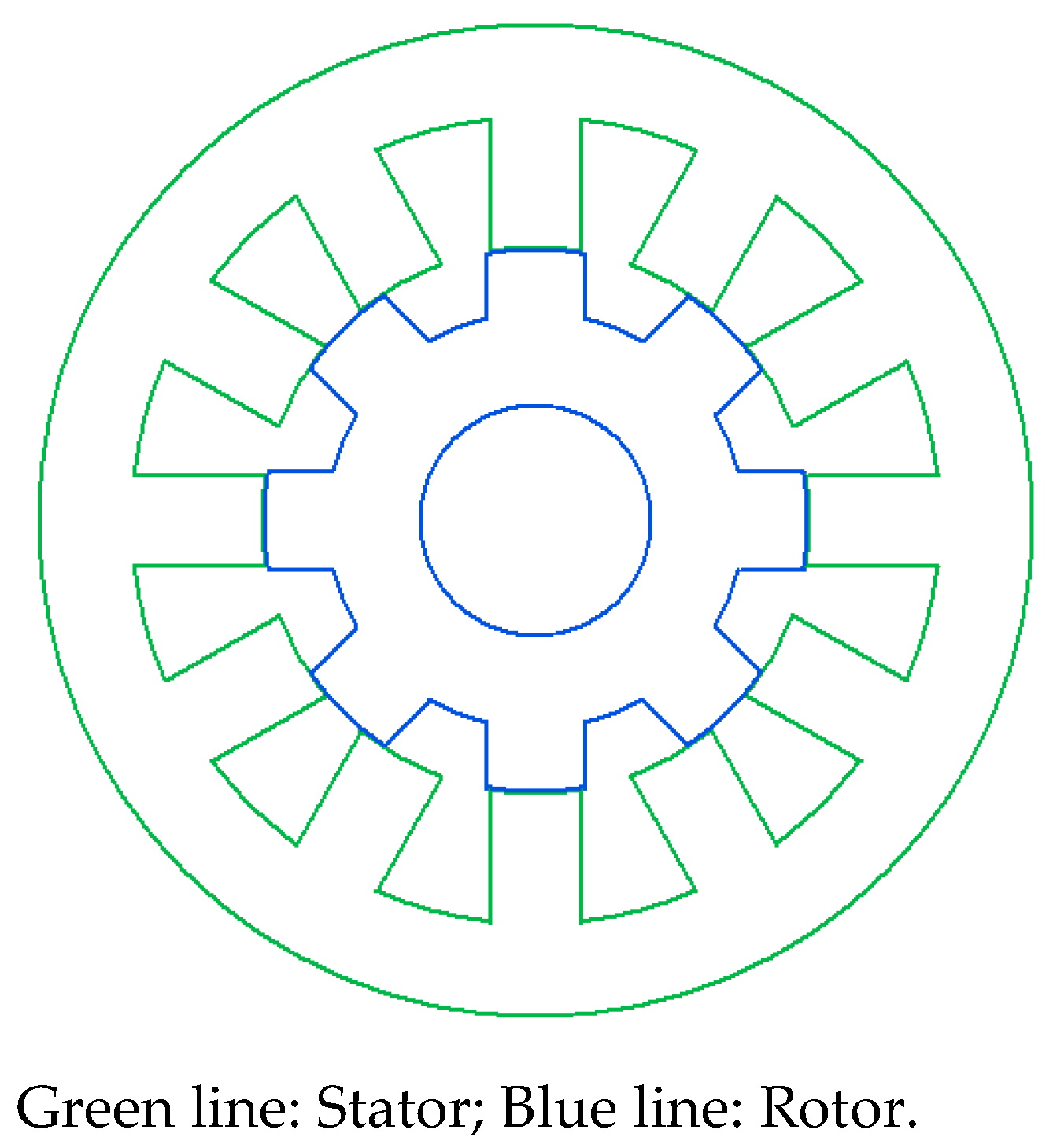
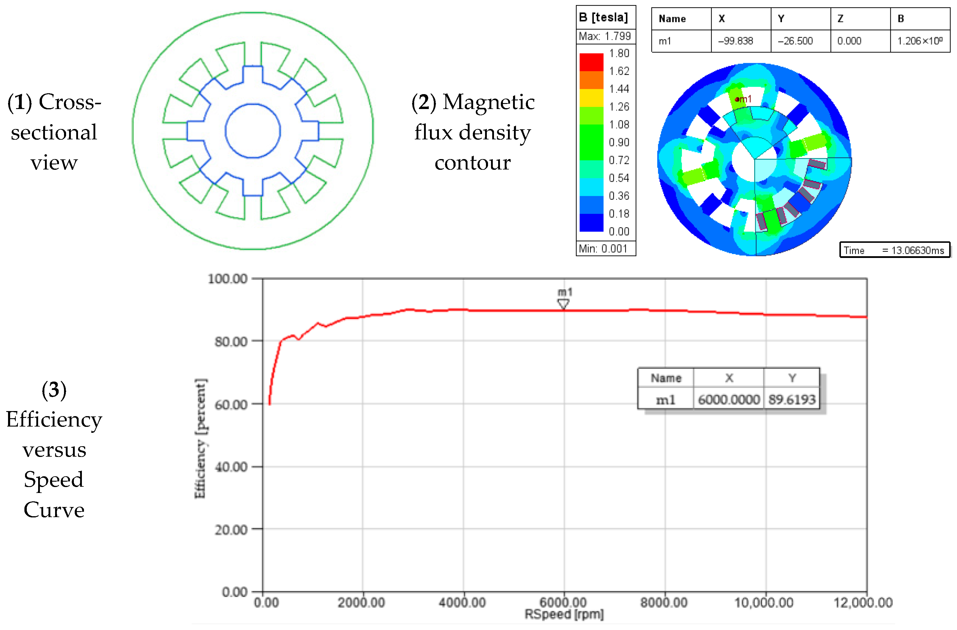
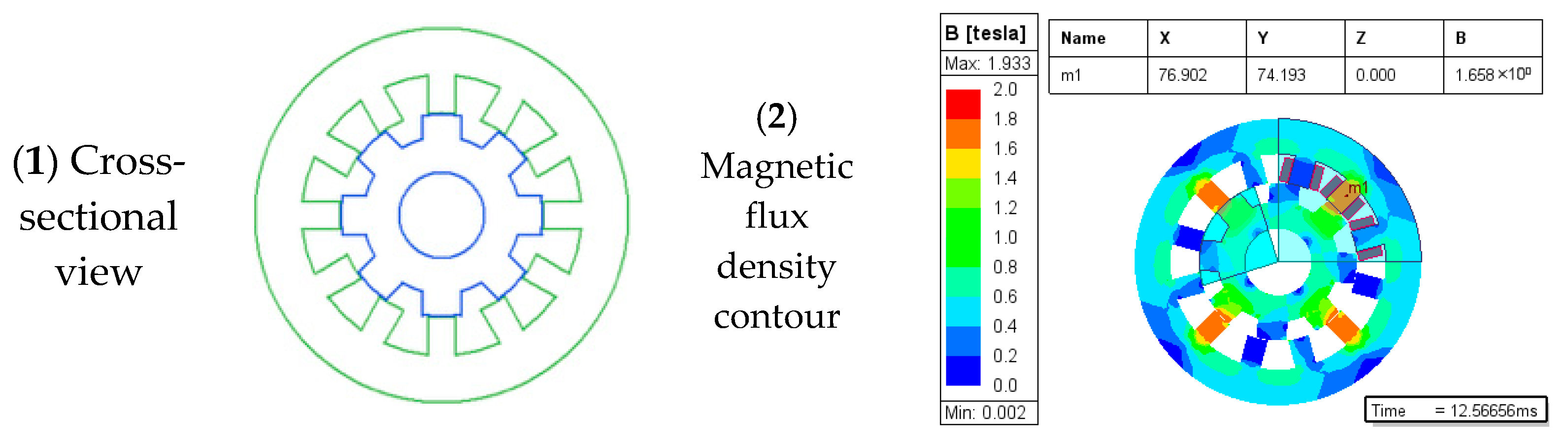
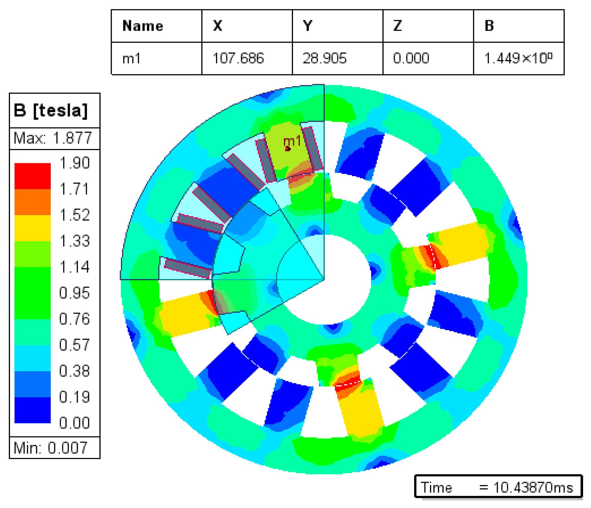
A 2D model of the motor was established using Ansys Maxwell, as illustrated in Figure 1. Figure 2 shows the magnetic flux density distribution contour of the motor.

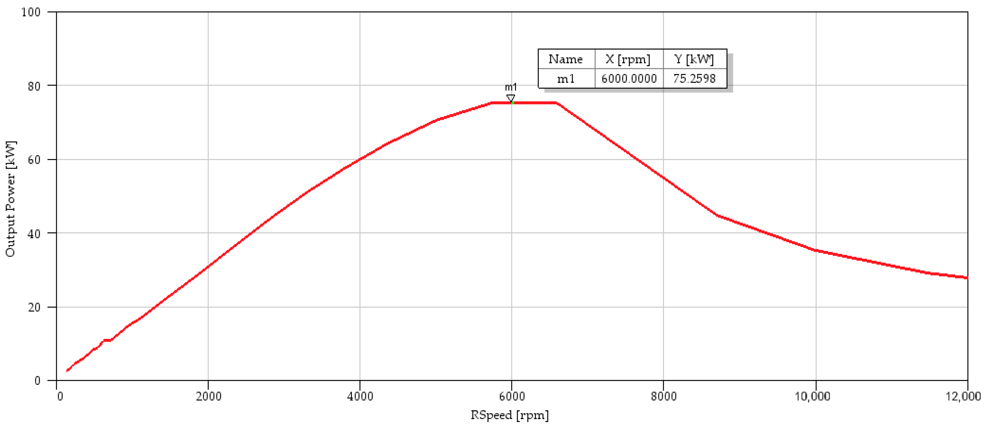
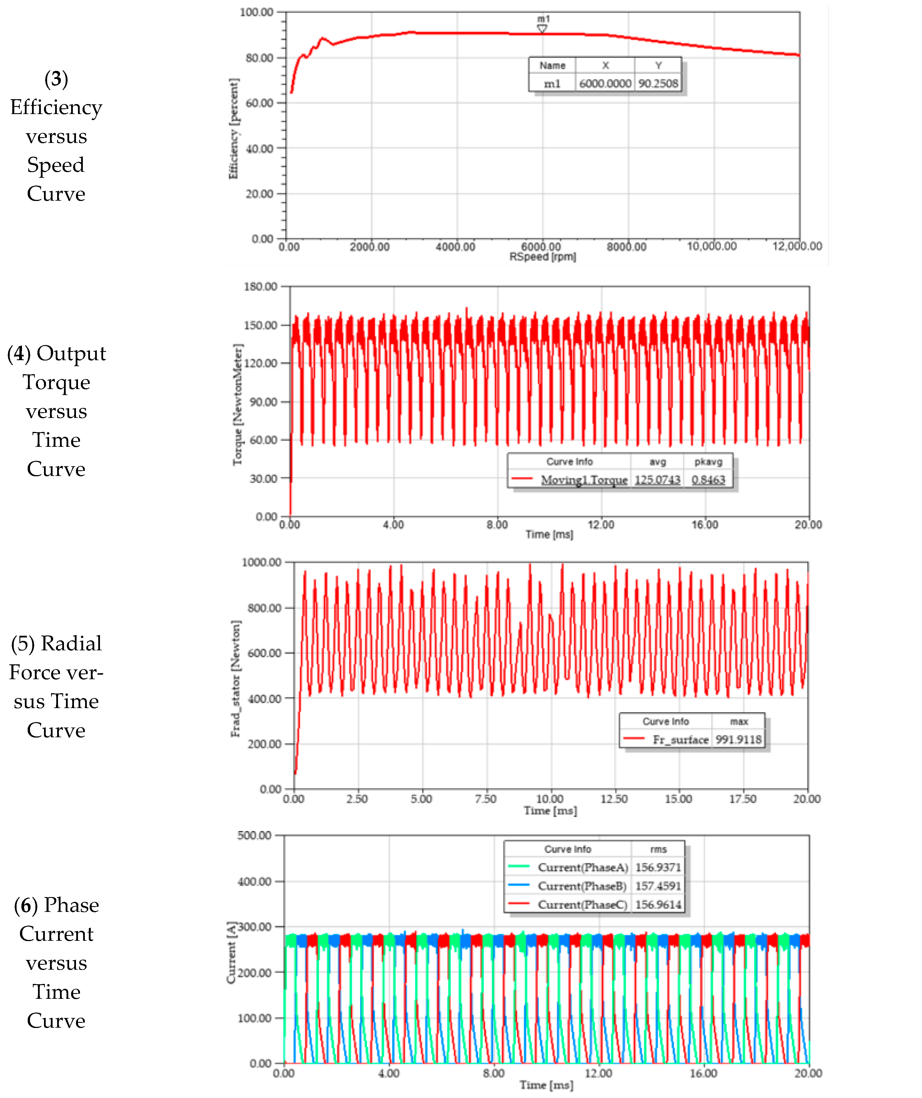
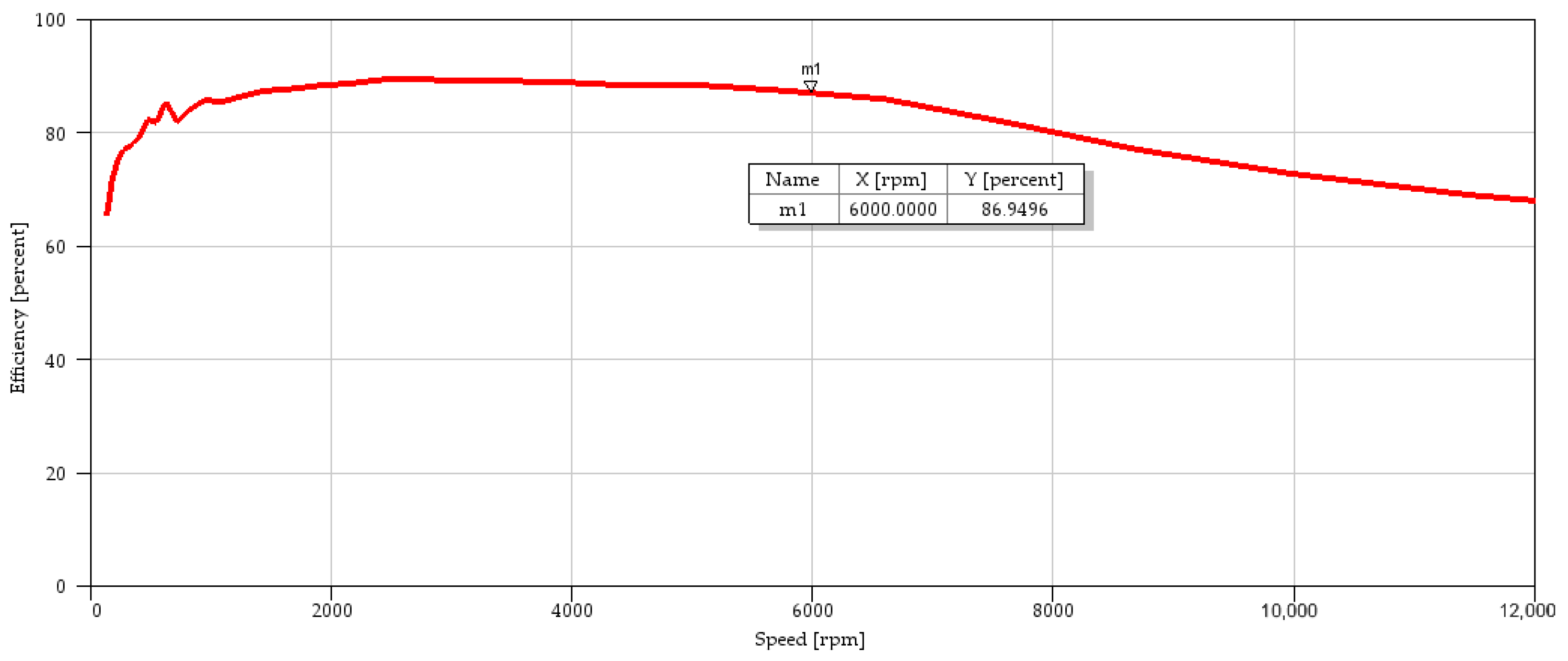
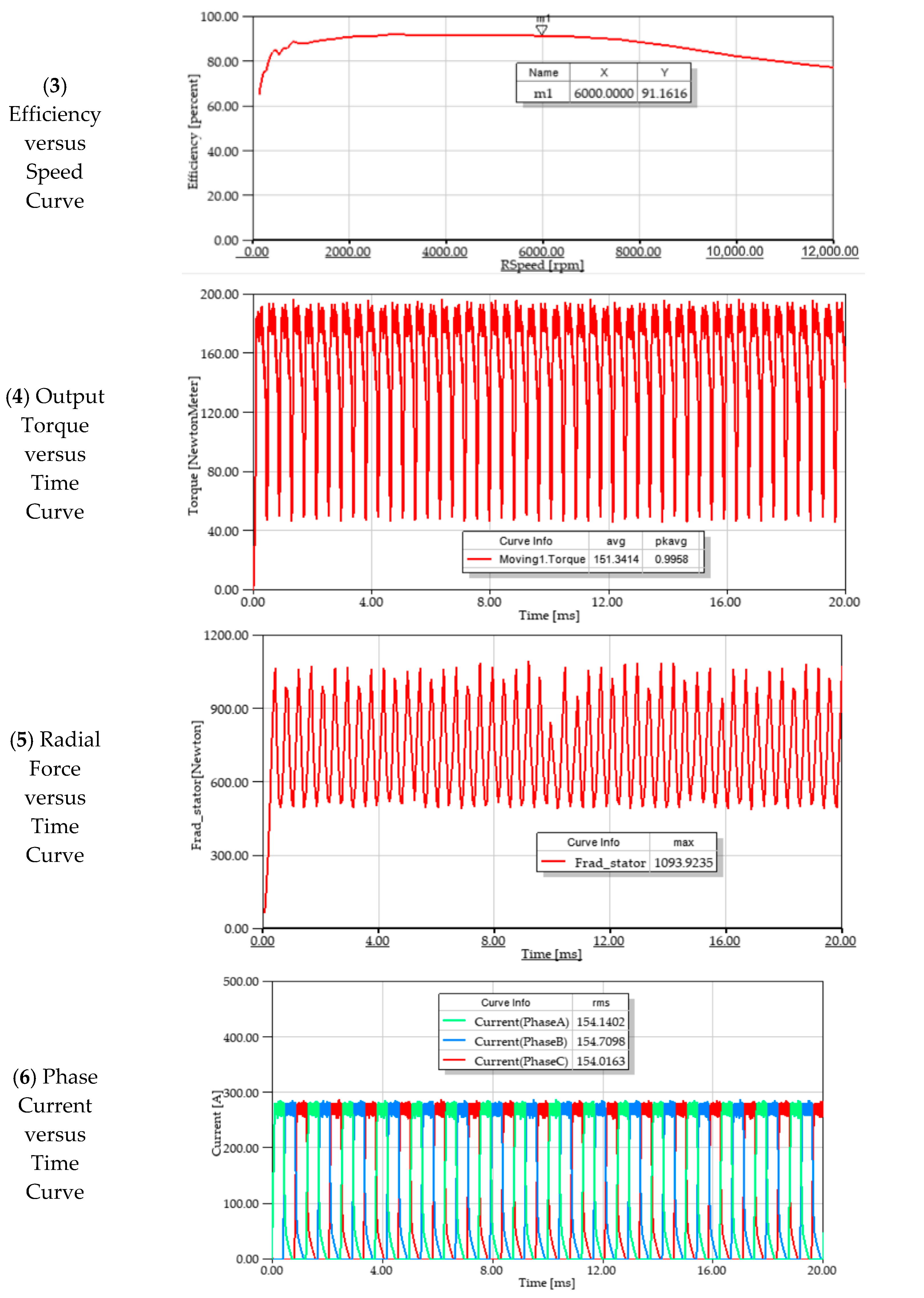
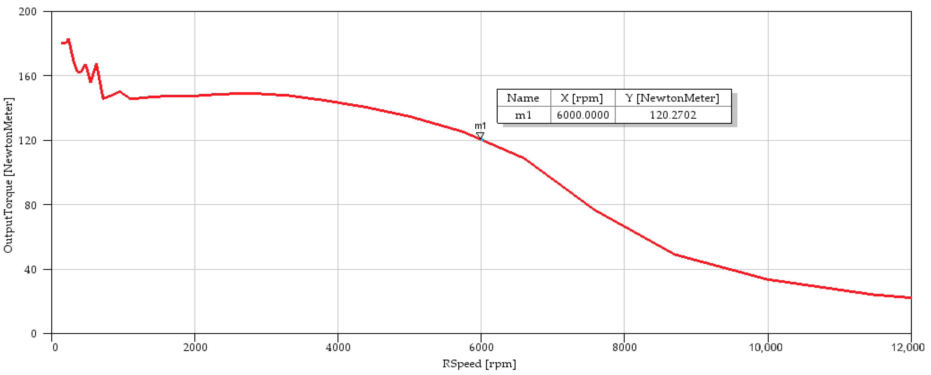
The motor was powered by an asymmetric half-bridge power converter circuit and controlled using the current chop control method, with a turn-on angle of −0.5° and a turn-off angle of 15.5°. At a speed of 6000 rpm, the motor achieved an efficiency of 87% (shown in Figure 3), an output power of 75.98 kW (shown in Figure 4), and an output torque of 120.92 N·m (shown in Figure 5).

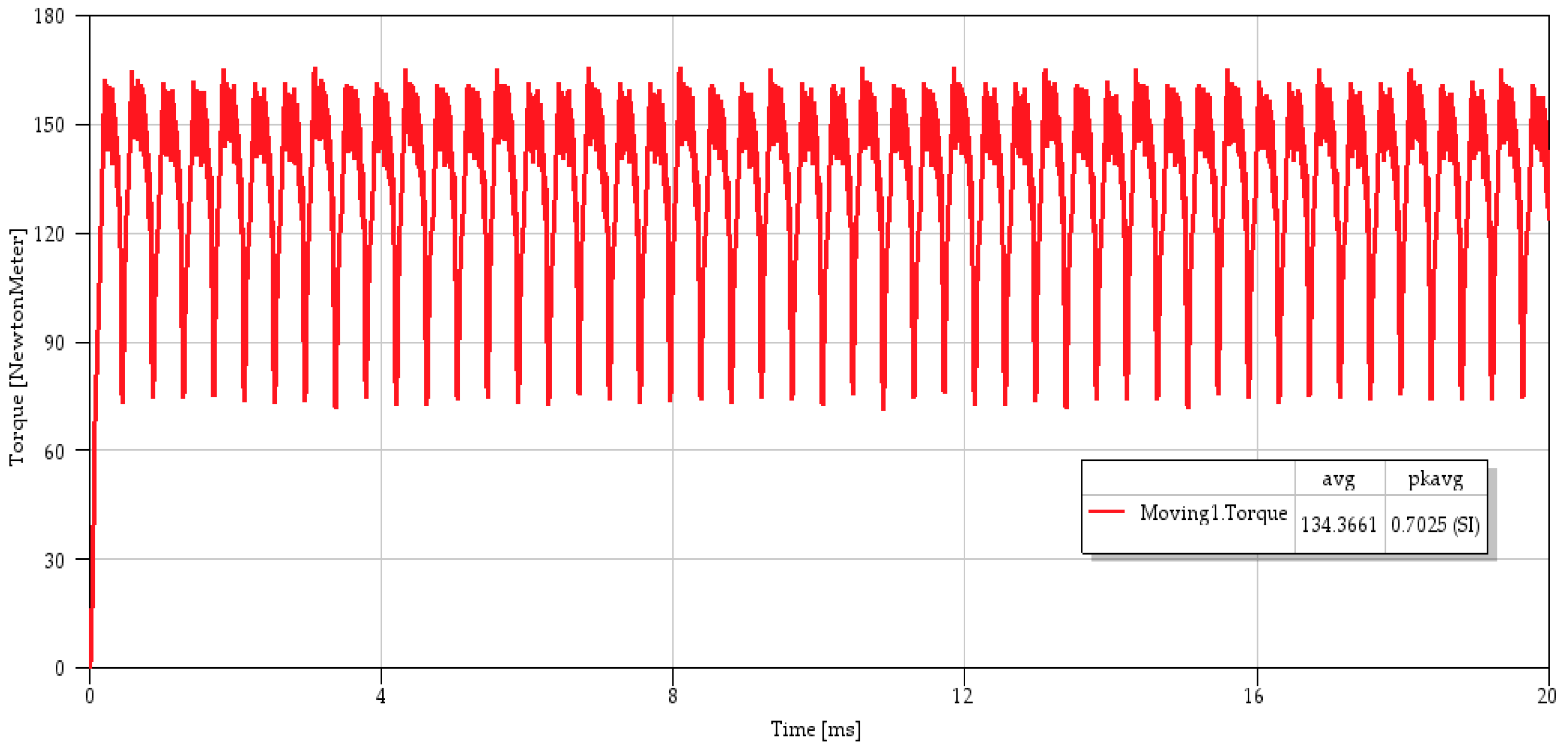
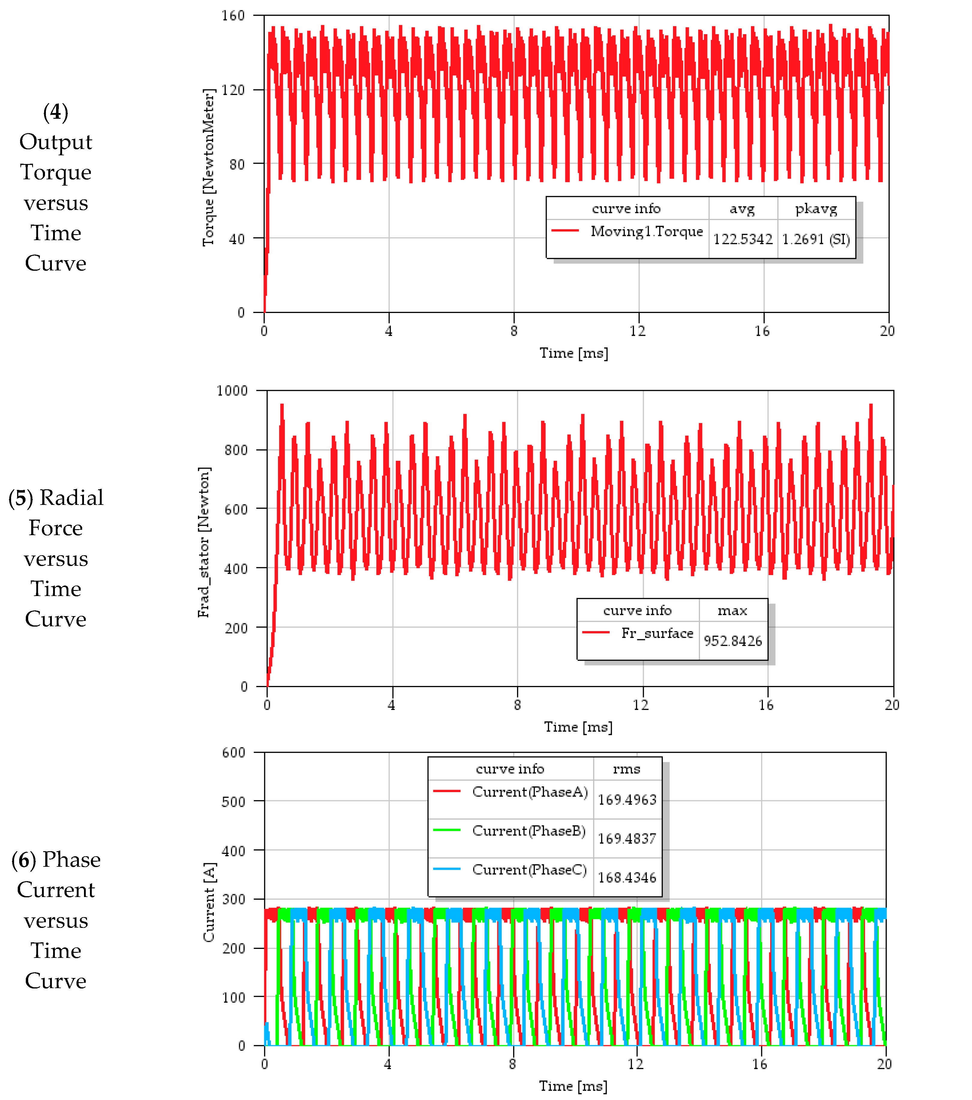
The electromagnetic torque curve of the motor in steady state in a two-dimensional transient simulation is shown in Figure 6. The average electromagnetic torque is 134.37 N·m, with a torque ripple (TRR) of 70.25%. The definition of torque ripple is provided in Formula (4) and can be calculated using Maxwell’s built-in function pkavg().

$$\mathrm{TRR}={\displaystyle \frac{T_{\max }-T_{\min }}{T_{\mathrm{avg}}}}\times 100\%=\mathrm{pkavg}\left(\right)\times 100\%$$

(4)

where $T_{\max }$, $T_{\min }$, and $T_{\mathrm{avg}}$ represent the maximum, minimum, and average torque values over one cycle, respectively.

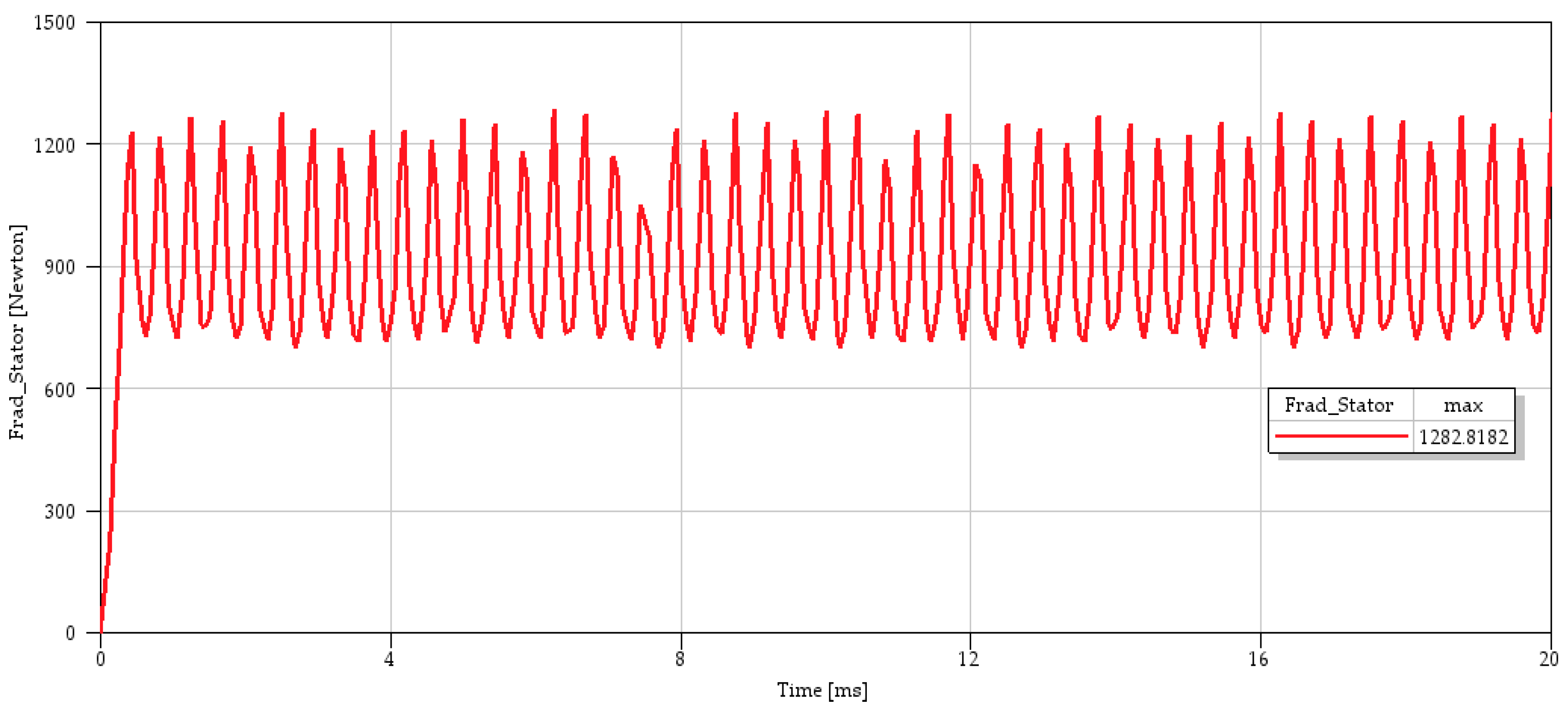
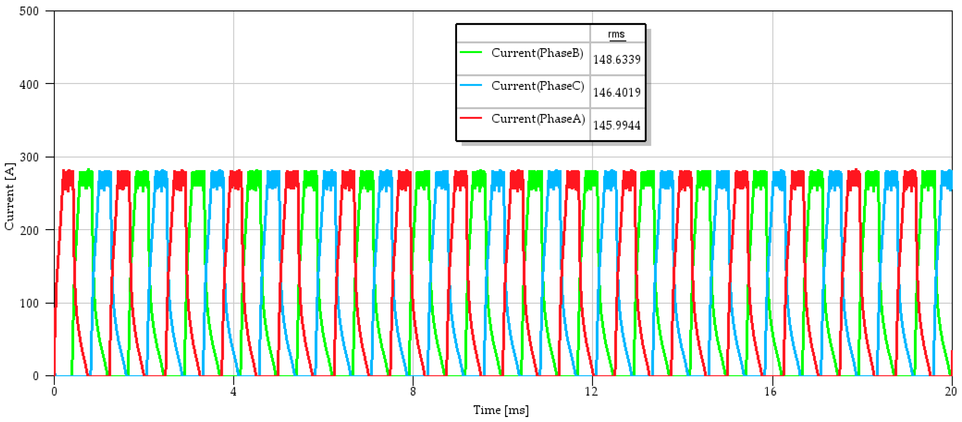
The radial force waveform acting on the salient stator pole surface is shown in Figure 7, exhibiting a maximum radial force amplitude of 1282.82 N. The radial force is calculated based on Maxwell’s stress tensor theory and can be obtained by manually defining the formula using the software’s built-in field calculator. At this time, the amplitude of the three-phase winding currents is constrained within the range of 260 A to 280 A, with an RMS value of approximately 146 A. The waveforms of the three-phase currents are depicted in Figure 8.

According to the results of the magnetic circuit and transient field simulations, all motor performance metrics, with the exception of efficiency, met the design requirements, while the efficiency was marginally below the target specification. The magnetic flux density contour plot in Figure 2 shows that at the peak flux linkage, the magnetic flux densities in the stator tooth tip and the stator tooth body reached 1.877 T and 1.449 T, respectively. This indicates an effective utilization of the magnetic material, albeit with significant saturation at the tooth tips. In addition, the amplitude of the radial force acting on the stator pole surface is relatively high; this serves as the main excitation source of mechanical vibration in the motor and should be further reduced. To address these issues, optimization methods are applied to improve the motor’s topology, thereby enhancing its overall performance.

2.2. Game-Theoretic Multi-Objective Design Optimization for Electric Machines

2.2.1. Traditional Multi-Objective Design Approach

(1) Selection of Optimization Objectives

The formulation of the objective function reflects the designer’s intent and the performance metrics of primary concern. When the design requirements are to reduce vibration and enhance load capacity, minimizing the radial electromagnetic force and maximizing the average electromagnetic torque are the optimization objectives. Here, the average electromagnetic torque $T_{\mathrm{avg}}$ and the peak radial electromagnetic force $\left|F_{\max }\right|$ were adopted as optimization metrics. Both values can be obtained through calculations performed in Ansys EM Suite 2023 R1 for motor simulation.

(2) Selection of Optimization Variables

The motor has numerous highly flexible structural parameters, making it impractical to optimize all of them comprehensively. Based on an analysis of the existing literature, the following structural variables are currently recognized to have a significant influence on motor performance: the stator pole arc coefficient ${\beta }_{\mathrm{s}}$, rotor pole arc coefficient ${\beta }_{\mathrm{r}}$, stator yoke height $h_{\mathrm{s}}$, and air gap length $g$ [20]. The other motor dimensions not mentioned here (such as the stator’s inner and outer diameters) will retain their initial design values. Therefore, any change in the air gap $g$ corresponds directly to an adjustment in the rotor’s outer diameter $D_r$.

Considering the feasibility of the finite element simulation, the value ranges of each variable are shown in

Table 2. The range of values for the optimization variables.

Parameter (Unit)	Lower Bound	Upper Bound
Stator pole arc coefficient, ${\beta }_{\mathrm{s}}$	0.5	0.75
Rotor pole arc coefficient, ${\beta }_{\mathrm{r}}$	0.35	0.5
Stator yoke height, $h_{\mathrm{s}}$ (mm)	15	40
Air gap length, $g$ (mm)	0.25	1

. The bounds of the design variables constitute the optimization constraints.

(3) The Mathematical Model for the Design Optimization Problem

By analyzing the motor optimization objectives and variables, the multi-objective optimization model is derived and expressed in Equation (5):

$$\left\{\begin{array}{l}findX=[{\beta }_{\mathrm{s}},{\beta }_{\mathrm{r}},h_{\mathrm{s}},g]\\ \min F(X)=[-T_{\mathrm{avg}},\left|F_{\max }\right|]\\ \mathrm{s}.\mathrm{t}.0.5\le {\beta }_{\mathrm{s}}\le 0.75,0.35\le {\beta }_{\mathrm{r}}\le 0.5,15\le h_{\mathrm{s}}\le 40,0.25\le g\le 1\end{array}\right.$$

(5)

where $X$ is the set of design variables and $F(X)$ is the set of optimization objectives. In addition to the upper and lower bound constraints on the optimization variables, the optimization model also satisfies the following two constraints:

➀ The variables ${\theta }_{\mathrm{s}}$ and ${\theta }_{\mathrm{r}}$, representing the pole arc angles of ${\beta }_{\mathrm{s}}$ and ${\beta }_{\mathrm{r}}$, respectively, are subject to the feasible triangle equation constraints as follows [6]:

$$\left\{\begin{array}{c}{\theta }_{\mathrm{s}}\le {\theta }_{\mathrm{r}}\\ {\theta }_{\mathrm{s}}+{\theta }_{\mathrm{r}}\le {\displaystyle \frac{360}{N_{\mathrm{r}}}}\\ {\displaystyle \frac{360}{m\cdot N_{\mathrm{r}}}}\le \min ({\theta }_{\mathrm{s}},{\theta }_{\mathrm{r}})\end{array}\right.$$

(6)

where $m$ and $N_{\mathrm{r}}$ represent the number of phases and the number of rotor poles, respectively.

➁ The average torque must be no less than 119 N·m, i.e., $T_{\mathrm{avg}}\ge 119$.

(4) Optimization Model Solution Methods

The standard weighted sum method (Equation (7)) is typically used for such multi-objective problems.

$$\min D(X)=w_1(-T_{\mathrm{avg}})+w_2\left|F_{\max }\right|$$

(7)

where $D(X)$ denotes the composite objective function, in which $w_1$ and $w_2$ represent designer-specified weighting factors. Integrating the optimization variable constraints and applying advanced optimization algorithms (e.g., particle swarm optimization (PSO)) enables the derivation of the optimal design variable set $\{{\beta }_{\mathrm{s}},{\beta }_{\mathrm{r}},h_{\mathrm{s}},g\}$.

The conventional weighted sum approach exhibits computational inefficiency and sensitivity to designer subjectivity. By reformulating the multi-objective optimization problem as a multi-agent game-theoretic decision problem, we can eliminate the need to manually assign weighting coefficients, reduce computational duration, and enhance problem-solving capability.

2.2.2. Transformation of Multi-Objective Optimization Problems into Game-Theoretic Formulations

According to game theory [13], a game $G$ can be represented as $G=〈m_{\mathrm{p}};\left\{T_i\right\}\left\{i\in m_{\mathrm{p}}\right\};\left\{u_i\right\}\left\{i\in m_{\mathrm{p}}\right\}〉$, where $m_{\mathrm{p}}$ denotes the set of players, $T_i$ represents the strategy space of player $i$, and $u_i$ is the payoff function for player $i$.

The method for transforming a multi-objective optimization problem into a game-theoretic formulation is as follows:

➀ Player mapping—each of the optimization objectives corresponds to each player in the game.

➁ Payoff function—the objective function is mapped to the player’s payoff function.

➂ Strategy space—the design variables define the strategy space for each player.

➃ Constraints—the feasible ranges of the design variables translate into constraints in the game.

Thus, the multi-objective optimization problem is reformulated in game-theoretic terms as follows:

$$G=〈T_{\mathrm{e}},F_{\mathrm{rad}};\left\{{\beta }_{\mathrm{s}},{\beta }_{\mathrm{r}},h_{\mathrm{s}},g\right\};\left\{T_{\mathrm{avg}},\left|F_{\max }\right|\right\}〉$$

(8)

where the electromagnetic torque $T_{\mathrm{e}}$ and radial electromagnetic force $F_{\mathrm{rad}}$ are regarded as players; the design variables ${\beta }_{\mathrm{s}}$, ${\beta }_{\mathrm{r}}$, $h_{\mathrm{s}}$, and $g$ form the strategy space; and the objective functions $T_{\mathrm{avg}}$ and $\left|F_{\max }\right|$ serve as the payoff functions. The feasible ranges of ${\beta }_{\mathrm{s}}$, ${\beta }_{\mathrm{r}}$, $h_{\mathrm{s}}$ and $g$ are the constraints of the game.

Here, the variables ${\beta }_{\mathrm{s}}$, ${\beta }_{\mathrm{r}}$, $h_{\mathrm{s}}$, and $g$ collectively form the strategy space of the entire game problem. However, these four variables and their different combinations have varying impacts on the game players. It is necessary to identify strategies that are strongly correlated with each player and construct their respective strategy spaces.

The specific steps include

➀ Solving single-objective optimal solutions;

➁ Calculating influence factors;

➂ Fuzzy clustering of influence factors;

➃ Allocating the strategy spaces for the two game players, $T_{\mathrm{e}}$ and $F_{\mathrm{rad}}$.

2.2.3. Determination of Strategy Spaces for Different Game Players

(1) Solving single-objective optimal solutions

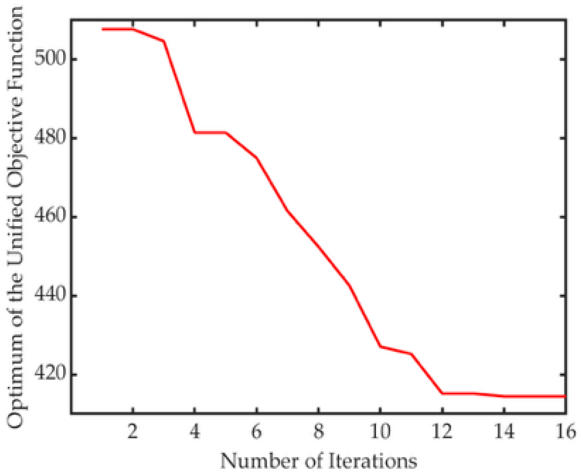
Co-simulation using MATLAB R2022a and Ansys EM Suite 2023 R1 was employed to obtain single-objective optimal solutions. In MATLAB, an optimization function was constructed and solved using the particle swarm optimization (PSO) algorithm. Each combination of design variables {${\beta }_{\mathrm{s}}$, ${\beta }_{\mathrm{r}}$, $h_{\mathrm{s}}$, $g$} is treated as a particle in the algorithm. The ANSYS Maxwell program is then called to assign these dimensional combinations to the established motor model for finite element analysis, which calculates the average electromagnetic torque value $T_{\mathrm{avg}}$. This torque value is returned to the MATLAB optimization algorithm as the particle’s fitness value for evaluation. This process is iteratively repeated until the dimensional combination yielding the maximum average electromagnetic torque is identified.

Using the aforementioned method, the optimization results corresponding to the maximum average electromagnetic torque $T_{\mathrm{avg}}$ are obtained as follows:

$$\begin{gathered} X_1^{*}=[0.6,0.41,32.78,0.25] \\ {T}_{\mathrm{avg}}=183.81\mathrm{N}·\mathrm{m} \end{gathered}$$

The optimization results for minimizing the maximum amplitude of radial force $\left|F_{\max }\right|$ are obtained as follows:

$$\begin{gathered} X_2^{*}=[0.50,0.35,40.00,0.55] \\ \left|F_{\max }\right|=895.02\mathrm{N} \end{gathered}$$

(2) Calculation of Influence Factor Matrix

Assuming the influence factor of design variable $x_j$ on objective function $f_i(X)$ is ${\mathsf{\Delta }}_{ji}$, if $f_i(X)$ is an implicit function of $x_j$, ${\mathsf{\Delta }}_{ji}$ can be computed using the finite difference method, as shown in Equation (9).

$${\Delta }_{ji}=\left.{\displaystyle \frac{\partial f_i}{\partial x_j}}\approx {\displaystyle \frac{f_i(x_j+\Delta x)-f_i(x_j)}{\Delta x}}\right|,i=1,2,\dots ,m_{\mathrm{p}};j=1,2,\dots ,n$$

(9)

where $n$ represents the number of design variables. In this study, the influence factors of the design variables {${\beta }_{\mathrm{s}}$, ${\beta }_{\mathrm{r}}$, $h_{\mathrm{s}}$, $g$} on the two optimization objectives {$T_{\mathrm{avg}}$,$\left|F_{\max }\right|$} are collectively expressed as matrix $\Delta$ (see Equation (10)).

$$\Delta =\left[\begin{array}{cc}358.2561& 2275.4\\ -2545.4& 2174.1\\ -0.1771& -0.00001\\ -144.898& 687.514\end{array}\right]$$

(10)

(3) Solution of Fuzzy Clustering Matrix

First, the shift-range transformation method (Equation (11)) is applied to normalize the influence factor matrix $\Delta$, yielding the standardized matrix ${\Delta }_1$, as shown in Equation (12)).

$${\Delta }_1={(x_{ij}^{\prime })}_{4\text{×}2}={({\displaystyle \frac{x_{ij}-\min \{\left.x_{ij}\right|1\le i\le 4\}}{\max \{\left.x_{ij}\right|1\le i\le 4\}-\min \{\left.x_{ij}\right|1\le i\le 4\}}})}_{4\text{×}2}$$

(11)

$${\Delta }_1=\left[\begin{array}{cc}1& 1\\ 0& 0.9555\\ 0.8766& 0\\ 0.8267& 0.3022\end{array}\right]$$

(12)

Next, the Euclidean distance method (Equation (13)) is employed to compute the fuzzy similarity matrix $R={(r_{ij})}_{4\text{×}4}$, as shown in Equation (14).

$$r_{ij}=1-cd(x_i^{\prime },x_j^{\prime })$$

(13)

Here, $d(x_i^{\prime },x_j^{\prime })=\sqrt{{\displaystyle \sum _{k=1}^2{(x_{ik}^{\prime }-x_{jk}^{\prime })}^2}}$, $c$ represents the correlation coefficient threshold (where higher values indicate greater similarity), which was set to 0.8 in this study.

$$R=\left[\begin{array}{cc}1& 0.1992\\ 0.1992& 1\\ 0.1939& -0.0373\\ 0.4248& 0.1570\end{array}\begin{array}{cc}0.1939& 0.4248\\ -0.0373& 0.1570\\ 1& 0.7550\\ 0.7550& 1\end{array}\right]$$

(14)

Subsequently, the transitive closure matrix $t(R)$ is obtained by taking the self-composition of matrix $R$, yielding the equivalence matrix $\overline{R}=t(R)$, as expressed in Equation (15):

$$\overline{R}=\left[\begin{array}{cc}1& 0.20\\ 0.20& 1\\ 0.42& 0.20\\ 0.42& 0.20\end{array}\begin{array}{cc}0.42& 0.42\\ 0.20& 0.20\\ 1& 0.76\\ 0.76& 1\end{array}\right]$$

(15)

Finally, the fuzzy clustering matrix $R_k$ is obtained by thresholding each element $r_{ij}$ in matrix $\overline{R}$ using the separation coefficient $k$, according to Equation (16):

$$r_{ij}^{\prime }=\left\{\begin{array}{cc}0& r_{ij}<k\\ 1& r_{ij}\ge k\end{array}\right.k\in [0,1]$$

(16)

Taking $k$ values of 1, 0. 76, 0.42, and 0.20 sequentially results in the four resulting clustering matrices shown in Equation (17):

$$\left\{\begin{array}{cc}{R}_1=\left[\begin{array}{cccc}1& 0& 0& 0\\ 0& 1& 0& 0\\ 0& 0& 1& 0\\ 0& 0& 0& 1\end{array}\right]& R_{0.76}=\left[\begin{array}{cccc}1& 0& 0& 0\\ 0& 1& 0& 0\\ 0& 0& 1& 1\\ 0& 0& 1& 1\end{array}\right]\\ R_{0.42}=\left[\begin{array}{cccc}1& 0& 1& 1\\ 0& 1& 0& 0\\ 1& 0& 1& 1\\ 1& 0& 1& 1\end{array}\right]& R_{0.20}=\left[\begin{array}{cccc}1& 1& 1& 1\\ 1& 1& 1& 1\\ 1& 1& 1& 1\\ 1& 1& 1& 1\end{array}\right]\end{array}\right.$$

(17)

(4) Determination of Strategy Space for Each Game Player

It is evident from Equation (17) that when the separation coefficient $k$ is 0.20, all design variables are grouped into one category: $\{{\beta }_{\mathrm{s}},{\beta }_{\mathrm{r}},h_{\mathrm{s}},g\}$. When the coefficient is 0.42, they can be divided into two categories: $\left\{{\beta }_{\mathrm{r}}\right\}$ and $\{{\beta }_{\mathrm{s}},h_{\mathrm{s}},g\}$. When the coefficient is 0.76, they are split into three categories: $\left\{{\beta }_{\mathrm{s}}\right\}$, $\left\{{\beta }_{\mathrm{r}}\right\}$, and $\{h_{\mathrm{s}},g\}$. When the coefficient is 1, they are classified into four categories.

Since there are two players, when the separation coefficient is set to 0.42, the strategy space $T_1$ for Player $T_{\mathrm{e}}$ is $\{{\beta }_{\mathrm{s}},h_{\mathrm{s}},g\}$, and the strategy space $T_2$ for Player $F_{\mathrm{rad}}$ is $\left\{{\beta }_{\mathrm{r}}\right\}$.

2.2.4. Formulation of the Payoff Function

Through a mapping process that converts design variables into the players’ strategy spaces, the initial strategy spaces are obtained by setting the design variables’ lower bounds as follows:

An initial strategy space $T^{\left(0\right)}=\left\{T_1^{\left(0\right)},T_2^{\left(0\right)}\right\}$ are defined as

$$\begin{gathered} T_1^{\left(0\right)}=\{{\beta }_{\mathrm{s}}^{\left(0\right)},h_{\mathrm{s}}^{\left(0\right)},g^{\left(0\right)}\}=\{0.50,15,0.25\} \\ {T}_2^{\left(0\right)}=\left\{{\beta }_{\mathrm{r}}^{\left(0\right)}\right\}=0.35 \end{gathered}$$

Therefore, the corresponding complementary spaces are defined as

$$\begin{gathered} {\overline{T}}_1^0={{\rm T}}_2^{\left(0\right)}=\left\{{\beta }_{\mathrm{r}}^{\left(0\right)}\right\} \left(\mathrm{Complement}\mathrm{of}{T}_1^{\left(0\right)}\right) \\ {\overline{T}}_2^0=T_1^{\left(0\right)}=\{{\beta }_{\mathrm{s}}^{\left(0\right)},h_{\mathrm{s}}^{\left(0\right)},g^{\left(0\right)}\} \left(\mathrm{Complement}\mathrm{of}{T}_1^{\left(0\right)}\right) \end{gathered}$$

Given the coexistence of cooperation and competition among the players, the payoff function $u_i$ for player $i$ can be formulated as Equation (18):

$$u_i=w_{ii}{\displaystyle \frac{f_i(T_i,\overline{T_i})}{f_i(T_i^{*},\overline{T_i})}}+{\displaystyle \sum _{j=1(j\ne i)}^{m_{\mathrm{p}}}{w}_{ij}\frac{f_j(T_i,\overline{T_i})}{f_j(T_i^{*},\overline{T_i})}}(i,j=1,2,\dots ,m_{\mathrm{p}})$$

(18)

where $w_{ii}$ is the weight coefficient that indicates the extent of the player’s involvement in the competition.

A larger value indicates more intense competition. Conversely, $w_{ij}$ represents the cooperative relationship. $T_i^{*}$ denotes the optimal solution in the player’s strategy space under single-objective optimization.

When $w_{ii}=1$ and $w_{ij}=0$, the total payoff $u$ in the completely non-cooperative game model is obtained as Equation (19):

$$u=u_1+u_2={\displaystyle \frac{f_1(T_1,{\overline{T}}_1)}{f_1(T_1^{*},{\overline{T}}_1)}}+{\displaystyle \frac{f_2(T_2,{\overline{T}}_2)}{f_2({\overline{T}}_2,T_2^{*})}}$$

(19)

This equation suggests that there exists a strategy space $\{T_1,T_2\}$ such that the payoffs of both players are as close as possible to the best payoffs achievable in their respective optimal strategy spaces, thereby maximizing the overall collective payoff. In this case, the total benefit cannot exceed 2. This also indicates that competition diminishes the returns for both parties, preventing them from achieving the optimal individual gains that would be possible in the absence of competition.

When $w_{ii}=0$ and $w_{ij}=1$, the total payoff $u$ in the completely cooperative game model is obtained as Equation (20):

$$u=u_1+u_2={\displaystyle \frac{f_1(T_2,{\overline{T}}_2)}{f_1({\overline{T}}_2,T_2^{*})}}+{\displaystyle \frac{f_2(T_1,{\overline{T}}_1)}{f_2(T_1^{*},{\overline{T}}_1)}}$$

(20)

This formula indicates that when the game reaches equilibrium, there exists a strategy space $\{T_1,T_2\}$ enabling both players’ payoffs to deviate from the worst-case outcome (i.e., the minimal payoff obtained when facing the opponent’s optimal strategy space), thereby maximizing the collective payoff. In this scenario, the total return will be no less than 2. This also demonstrates that cooperation benefits both parties, achieving a synergistic effect where “1 + 1 > 2”.

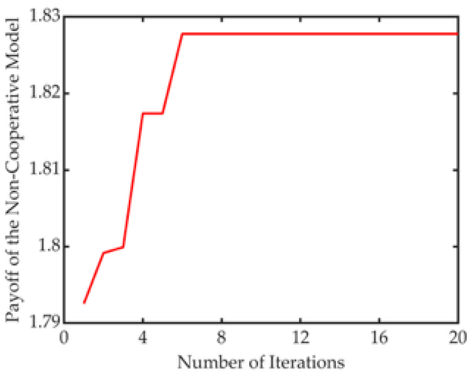
Combining with the motor optimization design problem discussed earlier in this paper, the completely non-cooperative game model is formulated, as shown in Equation (21):

$$\max u=u_1+u_2={\displaystyle \frac{T_{\mathrm{avg}}({\beta }_{\mathrm{s}},{\beta }_{\mathrm{r}},h_{\mathrm{s}},g)}{T_{\mathrm{avg}}({\beta }_{\mathrm{s}}^{*},{\beta }_{\mathrm{r}},h_{\mathrm{s}}^{*},g^{*})}}+{\displaystyle \frac{\left|F_{\max }({\beta }_{\mathrm{s}},{\beta }_{\mathrm{r}}^{*},h_{\mathrm{s}},g)\right|}{\left|F_{\max }({\beta }_{\mathrm{s}},{\beta }_{\mathrm{r}},h_{\mathrm{s}},g)\right|}}$$

(21)

The above equation demonstrates that when the game reaches equilibrium, the average electromagnetic torque will be maximized while the amplitude of the radial electromagnetic force is simultaneously minimized.

The fully cooperative game model for motor design optimization is presented in Equation (22):

$$\max u=u_1+u_2={\displaystyle \frac{T_{\mathrm{avg}}({\beta }_{\mathrm{s}},{\beta }_{\mathrm{r}},h_{\mathrm{s}},g)}{T_{\mathrm{avg}}({\beta }_{\mathrm{s}},{\beta }_{\mathrm{r}}^{*},h_{\mathrm{s}},g)}}+{\displaystyle \frac{\left|F_{\max }({\beta }_{\mathrm{s}}^{*},{\beta }_{\mathrm{r}},h_{\mathrm{s}}^{*},g^{*})\right|}{\left|F_{\max }({\beta }_{\mathrm{s}},{\beta }_{\mathrm{r}},h_{\mathrm{s}},g)\right|}}$$

(22)

Although it is expressed differently than Equation (20), this formula conveys the same fundamental physical meaning.

2.2.5. Solving Game-Theoretic Payoff Functions Using PSO

Particle swarm optimization (PSO) provides distinct advantages in solving the payoff function within the game-theoretic model of the aforementioned multi-objective motor design optimization. Compared to Genetic Algorithms (GAs) and Simulated Annealing (SA), PSO is often preferred due to its simplicity, fast convergence, and strong global search capability. The algorithm requires fewer parameters (mainly the inertia weight $w$, cognitive coefficient $c_1$, and social coefficient $c_2$), operates directly on real-valued vectors without complex genetic operations, exhibits inherent parallelism, and can effectively handle non-differentiable or discontinuous functions. With its straightforward parameter configuration, excellent convergence performance, and high computational efficiency, PSO is well-suited for addressing global optimization problems while meeting practical engineering requirements [22,23].

PSO is a population-based stochastic optimization technique inspired by the social behavior of birds flocking or fish schooling. In PSO, each potential solution is referred to as a “particle”. These particles traverse the search space, adjusting their positions and velocities based on their own experience (individual best solution, $pbest$) and the collective experience of the swarm (global best solution, $gbest$). The core idea is that particles stochastically oscillate within regions defined by $pbest$ and $gbest$, gradually converging toward the global optimum.

The standard PSO procedure consists of the following steps:

① Initialize the swarm: randomly generate a population of particles with initial positions and velocities.

② Evaluate fitness: calculate the fitness value for each particle according to the objective function.

③ Update $pbest$ and $gbest$: compare each particle’s current fitness with its personal best ($pbest$) and the swarm’s global best ($gbest$). Update $pbest$ and $gbest$ if better solutions are found.

④ Update velocity and position: for each particle, update its velocity and position using the velocity update formula (for a particle $i$ in the $d$ dimension),

$$v_{id}^{t+1}=w\cdot v_{id}^t+c_1\cdot r_1\cdot \left(pbes{t}_{id}-x_{id}^t\right)+c_2\cdot r_2\cdot \left(gbes{t}_d-x_{id}^t\right)r_1,r_2\in [0,1]$$

(23)

And the position update formula,

$$x_{id}^{t+1}=x_{id}^t+v_{id}^{t+1}(d=1,2,\dots ,n)$$

(24)

Here, $w$ represents the inertia weight, $c_1$ and $c_2$ are acceleration coefficients, $pbes{t}_{id}$ denotes the personal best position, $gbes{t}_d$ indicates the global best position, and $t$ is the iteration index.

⑤ Check the termination criteria: if stopping conditions are met (e.g., the maximum number of iterations is reached or the solution quality is satisfactory), terminate the process and output $gbest$; otherwise, return to Step ②.

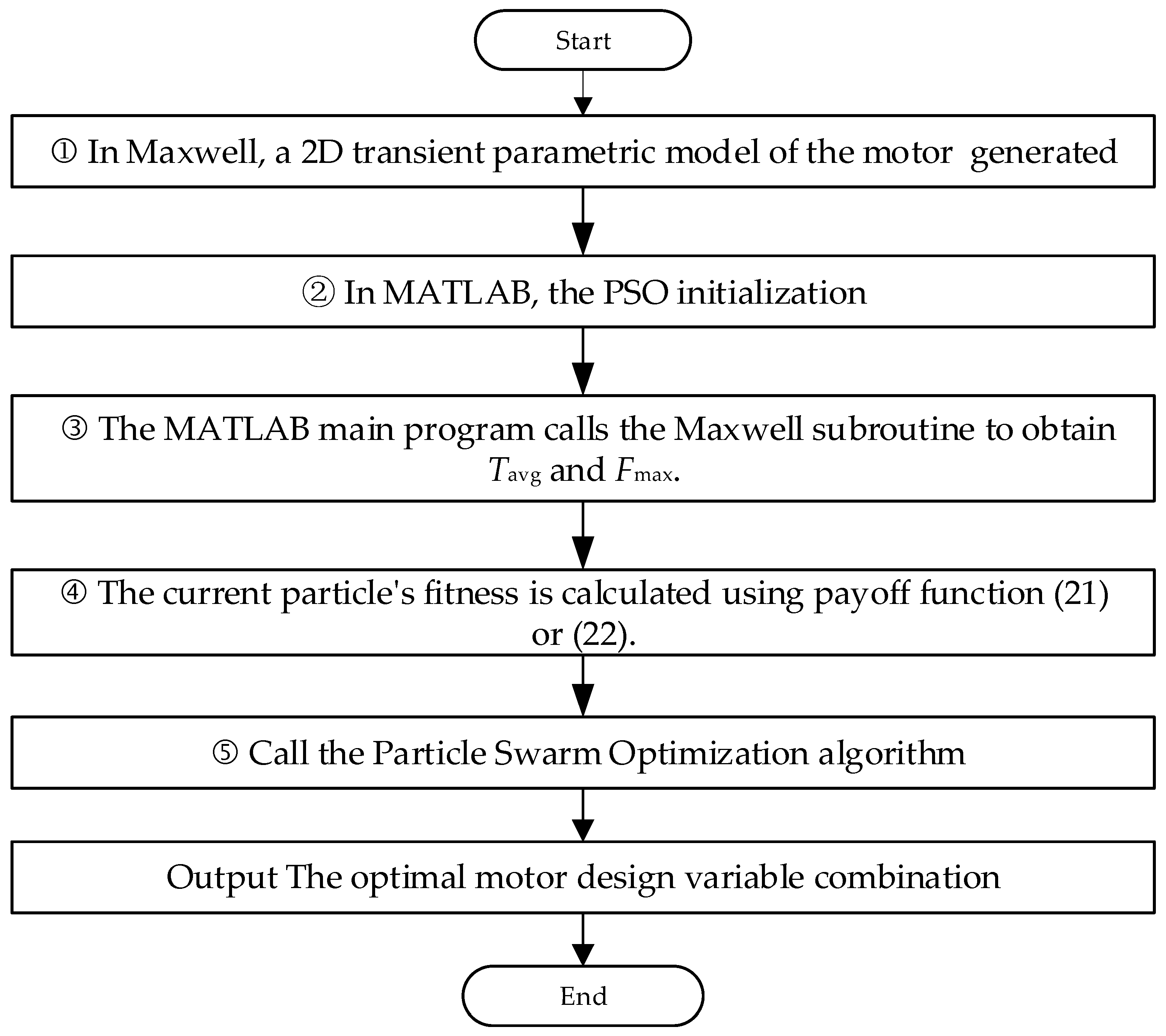
Based on this PSO framework, the optimal strategy space corresponding to the maximum payoff function, i.e., the most suitable combination of motor design variables, can be obtained through co-simulation using MATLAB and ANSYS Maxwell. The main steps of the optimization workflow are as follows:

① In Maxwell, a 2D transient parametric model of the motor is generated according to the initial design.

② In MATLAB, configure the particle swarm parameters including population size, initial particle velocities and positions, update formula coefficients, and maximum iteration count.

③ The Maxwell program is called to assign the current particle’s position to the motor dimensional variables, perform 2D transient FEA simulation, and return the average electromagnetic torque and maximum radial electromagnetic force amplitude on the stator salient surface to the MATLAB program.

④ Based on the returned average electromagnetic torque and radial electromagnetic force amplitude, the overall payoff value is calculated using payoff function (21) or (22), which simultaneously represents the current particle’s fitness.

⑤ Referring to the standard PSO procedure, iterations are repeated until the stopping criteria are met, thereby obtaining the optimal result.

The aforementioned process can be described by the simplified flowchart below, as shown in Figure 9.

3. Results and Discussion

3.1. Optimization Results of Unified Objective Method

Since the average electromagnetic torque of the motor and the maximum amplitude of the radial electromagnetic force on the stator’s salient surface are of comparable orders of magnitude, weighting coefficients of 0.5 are assigned to each objective, resulting in a unified multi-objective function shown as Equation (25):

$$\min D=0.5\cdot (-T_{\mathrm{avg}})+0.5\cdot \left|F_{\max }\right|$$

(25)

Using the algorithmic workflow illustrated in Figure 9, the optimal motor design dimensions were determined to be $\{0.5,0.4,40,0.68\}$, with a corresponding optimal function value of 414.4137. The iterative optimization process, shown in Figure 10, converged to the optimal solution after 14 iterations.

3.2. Results of the Game Model

Following the algorithmic workflow depicted in Figure 9, compromise solutions were derived for both ➀ the non-cooperative game payoff function (Equation (21)) maximization, and ➁ the cooperative game payoff function (Equation (22)) maximization.

The optimization processes for both approaches are depicted in Figure 11 and Figure 12. The non-cooperative game algorithm converged after 7 iterations, producing compromise motor design parameters $\{0.51,0.49,37.21,0.25\}$ that achieved a collective payoff of 1.8278. In contrast, the cooperative game algorithm reached an equilibrium solution $\{0.51,0.49,39.81,0.59\}$ in 7 iterations, resulting in motor design variables that yielded a higher collective payoff of 2.4715. These simulated outcomes align closely with the theoretical predictions from Equations (19) and (20): the non-cooperative payoff remains below 2, while the cooperative strategy produces a payoff exceeding 2. The results thus provide empirical validation of the theoretical framework.

3.3. Verification Using ANSYS Parametric FEA

The motor design variable combinations obtained using the unified objective method, completely non-cooperative game algorithm, and completely cooperative game algorithm were each substituted into the parameterized 2D motor model in ANSYS Maxwell. The resulting motor cross-sectional topologies are shown in Figure 13(1), Figure 14(1) and Figure 15(1). Transient electromagnetic field simulations were conducted for each configuration, and the flux density cloud diagrams corresponding to each type of motor are presented in Figure 13(2), Figure 14(2) and Figure 15(2).

When the stator and rotor salient poles are aligned, in the motor topology obtained using the weighted method (Figure 13(2)), the flux density in the stator teeth is 1.2 Tesla, indicating no overall saturation except for localized saturation at the tooth tips. In the motor topology optimized using non-cooperative game theory (Figure 14(2)), the stator tooth body is mildly saturated with a magnetic flux density of 1.68 T, while more severe saturation occurs at the stator tooth tip. No saturation is observed in the rotor. Compared to the model derived from non-cooperative game theory, the cooperative game-based model exhibits a similar level of mild saturation in the stator tooth body. However, the saturation at the tips of both the stator and rotor teeth is slightly more severe.

Furthermore, performance comparison of the three motor types yielded the following conclusions. In terms of efficiency, the motor designed using the unified objective method (Figure 13(3)) achieved the lowest efficiency of 89.62%, whereas the motor obtained through non-cooperative game theory (Figure 14(3)) exhibited the highest efficiency, measured at 91.16%. Regarding electromagnetic torque performance, the motor designed via non-cooperative game theory (Figure 15(4)) demonstrated the maximum average electromagnetic torque of 151.34 N·m, along with a relatively high torque ripple of 99.58%. In contrast, the motor designed using the unified objective theory (Figure 14(4)) showed the minimum average electromagnetic torque, measuring 122.53 N.m, and the maximum torque ripple, reaching 126.91%. As for the radial electromagnetic force, the motor designed using the unified objective theory (Figure 15(5)) presented the minimum radial electromagnetic force amplitude at 952.84 N, while the motor obtained via non-cooperative game theory (Figure 14(5)) exhibited the maximum amplitude, measured at 1093.92 N. From the perspective of current waveforms, the motor based on non-cooperative game theory (Figure 15(6)) had the minimum RMS current of 154 A, whereas the motor designed with the unified objective method (Figure 13(6)) had the maximum RMS current at 169.5 A.

Based on the above analysis, among the three motor models, the one based on the unified objective method exhibited the highest winding current. However, it demonstrated a relatively low magnetic flux density in the stator tooth body, resulting in underutilization of the magnetic material. Consequently, this model suffers from high copper loss and relatively low efficiency. Furthermore, it produces the lowest electromagnetic torque and the largest torque ripple. In contrast, the model derived from non-cooperative game theory achieved the highest electromagnetic torque with a relatively low winding current, indicating efficient material utilization. However, more severe saturation at the stator and rotor tooth tips led to a larger radial electromagnetic force. Conversely, the cooperative game-based model delivered a performance that lay between the other two. It generated a relatively high electromagnetic torque with a low winding current, maintained good material utilization, and kept both the torque ripple and the amplitude of the radial electromagnetic force at acceptably low levels.

All three motor models are feasible and meet the core design specifications. The cooperative and non-cooperative game-based models are superior in terms of magnetic material utilization. For applications requiring a higher torque overload margin under rated conditions, the non-cooperative game-based model is recommended. When paired with a suitable control strategy, it can achieve the 119 N·m rated torque at the rated speed. If the operational focus is strictly on steady-state performance at the rated point, the cooperative game-based model offers a more balanced and preferable solution.

Given its balanced performance, the motor model derived from cooperative game theory is the recommended choice in this work. Its finalized design parameters are presented in

Table 3. Recommended Design Parameters of the Cooperative Game-Based Motor Model.

Parameter (Unit)	Value	Parameter (Unit)	Value
Stator outer diameter $D_{\mathrm{s}}$ (mm)	327	Stator inner diameter $D_{\mathrm{si}}$ (mm)	177
Stator yoke height $h_{\mathrm{s}}$ (mm)	39.81	Stator pole embrace ${\beta }_{\mathrm{s}}$	0.51
Rotor outer diameter $D_{\mathrm{r}}$ (mm)	175.82	Rotor inner diameter $D_{\mathrm{ri}}$ (mm)	75
Rotor yoke height $h_{\mathrm{r}}$ (mm)	34	Rotor pole embrace ${\beta }_{\mathrm{r}}$	0.49
Core stack length $l_{\mathrm{stk}}$ (mm)	174	Core material	M19_24G
Air gap length $g$ (mm)	0.59

.

3.4. Discussion

To address the deficiencies of the initial design in certain performance indicators, this paper adopted a parameter optimization method to enhance the overall performance of the system. Given the large number of motor design parameters, four key parameters were selected to reduce optimization dimensionality and achieve rapid design. Three different optimization models were constructed: a unified objective model (weighted sum model), a competitive game model, and a cooperative game model. The particle swarm optimization algorithm was applied to optimize the four-dimensional continuous solution space, with each optimization process demonstrating advantages of fast convergence and a low number of iterations. Corresponding optimized design parameters were ultimately obtained, and three different topological design schemes were generated accordingly.

To demonstrate the advantages of the method proposed in this paper, a comparison was made with the commonly used NSGA-II multi-objective optimization approach. Figure 16 shows the Pareto solution set obtained by NSGA-II after 20 generations of evolution. Among the solutions, the one that satisfied a torque greater than the rated value (119 N·m) and exhibited the smallest radial electromagnetic force amplitude—specifically {0.61, 0.44, 37.63, 0.7}—was selected as the Pareto solution. For this solution, the radial electromagnetic force amplitude was 1213 N, which was significantly higher than the corresponding performance indicators of the three motor designs presented earlier. In terms of iteration count, NSGA-II requires more iterations than all three methods proposed in this paper. Moreover, when the obtained solution was applied to the parametric motor model, the resulting performance indicators were not satisfactory. It is evident that the game-theory-based motor design optimization method achieved favorable results with fewer optimization steps and a faster convergence process.

In addition, from an engineering design standpoint, the game model constructed in this study still has room for further refinement. Currently, we used average electromagnetic torque as the optimization objective and employed control strategies to operate the motor near the working point. However, for applications with a fixed rated power, a more industrially relevant approach may involve setting the required torque as a fixed constraint, shifting the optimization focus toward maximizing torque density (to reduce material costs) and minimizing electromagnetic vibration (to improve acoustic performance). Therefore, constructing a multi-objective game optimization model that better aligns with industrial practical needs will be a key direction for our future research.

Although the currently constructed game model requires relatively few iterations during the optimization process, its performance data still relies on finite element simulations, resulting in a lengthy motor design cycle. To enhance the practicality of this method, developing a high-fidelity surrogate model capable of rapidly predicting motor performance will be a critical task for the future. Integrating multi-objective optimization methods with such surrogate models could significantly shorten the motor design time and better meet the industry’s demand for efficient and agile development processes.

4. Conclusions

The electromagnetic optimization of switched reluctance motors (SRMs) is inherently a high-dimensional, strongly nonlinear multi-objective design problem. Targeting the compressor drive motor as the optimization object, this study reconstructed the multi-objective design paradigm from a game-theoretic perspective: mapping the conflicting optimization objectives of average torque and radial electromagnetic force as agents in the game, with their strategy space objectively partitioned through fuzzy clustering algorithms and correlation analysis of continuous design variables. This approach establishes two novel types of payoff function models based on non-cooperative and fully cooperative games. The particle swarm optimization (PSO) algorithm is employed to search for equilibrium solutions within this continuous strategy space. The proposed optimization model overcomes the subjectivity in weight selection inherent in traditional weighted-sum methods and the limitations of discrete variable combinations.

Finite element simulation results demonstrate that this theoretical framework effectively characterize the conflict relationships among objectives within a continuous solution space, with the game-theoretic model ultimately achieving an optimal balance between torque output and vibration suppression. Compared to the initial design and other optimization methods, the cooperative and non-cooperative approaches better utilize magnetic materials and satisfies the operational requirements of air compressor applications. In such a scenario, either one may be selected as the design solution based on specific requirements. This research provides a concrete theoretical modeling method and solution mechanism for multi-objective optimization in motor design, ensuring a systematic design process and equilibrium solutions.