Article

Analysis of the Travelling Time According to Weather Conditions Using Machine Learning Algorithms

by
Gülçin Canbulut
Industrial Engineering Department, Nuh Naci Yazgan University, Erkilet 38030, Kayseri, Turkey
Appl. Sci. 2026, 16(1), 6; https://doi.org/10.3390/app16010006
Submission received: 7 October 2025 / Revised: 3 November 2025 / Accepted: 10 November 2025 / Published: 19 December 2025

Abstract

A large share of the global population now lives in urban areas, which creates growing challenges for city life. Local authorities are seeking ways to enhance urban livability, with transportation emerging as a major focus. Developing smart public transit systems is therefore a key priority. Accurately estimating travel times is essential for managing transport operations and supporting strategic decisions. Previous studies have used statistical, mathematical, or machine learning models to predict travel time, but most examined these approaches separately. This study introduces a hybrid framework that combines statistical regression models and machine learning algorithms to predict public bus travel times. The analysis is based on 1410 bus trips recorded between November 2021 and July 2022 in Kayseri, Turkey, including detailed meteorological and operational data. A distinctive aspect of this research is the inclusion of weather variables—temperature, humidity, precipitation, air pressure, and wind speed—which are often neglected in the literature. Additionally, sensitivity analyses are conducted by varying k values in the K-nearest neighbors (KNN) algorithm and threshold values for outlier detection to test model robustness. Among the tested models, CatBoost achieved the best performance with a mean squared error (MSE) of approximately 18.4, outperforming random forest (MSE = 25.3) and XGBoost (MSE = 23.9). The empirical results show that the CatBoost algorithm consistently achieves the lowest mean squared error across different preprocessing and parameter settings. Overall, this study presents a comprehensive and environmentally aware approach to travel time prediction, contributing to the advancement of intelligent and adaptive urban transportation systems.

1. Introduction

Urbanization has intensified mobility challenges worldwide, particularly in large metropolitan areas where congestion, passenger density, and environmental variability jointly influence daily commuting patterns. The growing number of people living in cities increases traffic density and travel time, which directly reduces the quality of urban life. Local authorities and public transport operators therefore seek effective strategies to enhance transport efficiency, improve service quality, and support sustainable mobility. Among these strategies, accurate travel time prediction plays a crucial role in managing operations, optimizing schedules, and improving passenger satisfaction.
Public bus travel time estimation has become a key component of intelligent transportation systems (ITSs), providing data-driven support for decision-making and dynamic planning. A wide variety of methods—ranging from traditional mathematical and statistical models to advanced machine learning algorithms—have been developed for this purpose. Statistical regression models are easy to interpret but often fail to capture the non-linear and dynamic nature of urban transportation data. Conversely, machine learning models such as random forest, gradient boosting, or deep neural networks offer higher predictive accuracy but tend to require large datasets and may suffer from limited interpretability.
Despite the growing research in this area, most existing studies focus primarily on operational and traffic-related variables, such as route geometry, passenger count, or departure intervals, while environmental factors such as weather conditions remain largely underexplored. Yet, weather variables—temperature, humidity, precipitation, air pressure, and wind speed—significantly affect vehicle performance, road friction, and passenger behavior. The neglect of these factors limits the robustness and generalizability of many predictive models.
Recent developments in travel time prediction have increasingly relied on ensemble and deep learning models designed to enhance temporal accuracy and dynamic adaptability. These approaches primarily focus on short-term traffic fluctuations and sequential patterns, while environmental variables such as weather conditions are often overlooked. Earlier regression-based approaches, though more interpretable and computationally efficient, tend to lose accuracy under conditions of high variability or nonlinear relationships. Consequently, there remains a methodological gap between models that prioritize interpretability and those that achieve higher predictive flexibility, highlighting the need for an integrated framework that balances both dimensions.
To address this gap, the present study proposes a hybrid modeling framework that integrates statistical regression and machine learning algorithms for predicting public bus travel times. The study explicitly incorporates meteorological variables—temperature, humidity, air pressure, precipitation, and wind speed—to assess their impact on travel time estimation. Furthermore, model robustness is tested through sensitivity analyses by varying k values in the K-nearest neighbors (KNN) algorithm and adjusting threshold values for outlier detection.
This integrated framework contributes to both methodological development and practical decision-making in urban transport planning. By combining interpretability with high predictive accuracy, the study offers a more comprehensive and environmentally aware approach to travel time prediction.
From a theoretical perspective, meteorological variability can influence travel time through multiple mechanisms. Temperature and humidity affect engine efficiency and passenger comfort, influencing vehicle acceleration and boarding durations. Precipitation and wind speed alter road surface friction, reduce visibility, and lower driving speeds, while changes in air pressure are often correlated with weather fronts that modify traffic flow dynamics. These factors interact with operational variables—such as route geometry and departure intervals—to produce nonlinear fluctuations in travel time. Therefore, integrating meteorological parameters into predictive frameworks provides a physically and behaviorally grounded representation of transportation system performance under varying environmental conditions.
Accordingly, this study aims to answer the following research question: Does the inclusion of meteorological variables significantly improve the accuracy and robustness of public bus travel time prediction models?
Based on this, the research hypothesis is formulated as follows:
H1:
Integrating weather-related parameters such as temperature, humidity, precipitation, air pressure, and wind speed enhances model performance compared to models relying solely on operational and temporal data.
This explicit formulation clarifies the analytical focus of the study and establishes a clear link between the research objective, methodological framework, and empirical evaluation.
The remainder of this paper is organized as follows: Section 2 reviews the related literature, Section 3 explains the methodology and modeling framework, Section 4 presents the application and results, and Section 5 discusses findings and future research directions.

2. Literature Review

Travel time prediction has been a widely explored topic in the field of intelligent transportation systems (ITSs). Numerous studies have investigated different modeling approaches—ranging from traditional statistical methods to advanced machine learning (ML) algorithms—to improve the accuracy and robustness of travel time estimation. Table 1 summarizes representative studies in this field.
Machine learning models have become dominant in recent years due to their ability to capture nonlinear and complex relationships among traffic and temporal variables.
Serin et al. [1] applied ensemble learning models—AdaBoost, gradient boosting, random forest, Extra-Tree Regression, KNN, and SVM—to predict bus travel times in Istanbul, demonstrating that ensemble methods outperform single algorithms. Gal et al. [2] developed a hybrid model combining queueing theory and ML to enhance predictive reliability using real-world city data. Peterson et al. [3] introduced an LSTM-based framework capable of learning non-static spatio-temporal dependencies in bus networks, offering improved accuracy compared to traditional methods. Bai et al. [4] integrated support vector machines and Kalman filtering, where SVM predicted travel times and Kalman filtering refined the estimates using real-time data. Treethidtaphat et al. [5] proposed a deep neural network (DNN) model to predict bus arrival times and benchmarked it against the Ordinary Least Squares (OLS) regression, achieving superior results. Chen et al. [6] designed an intelligent transport system using nine algorithms, including linear regression, KNN, SVR, gradient boosting, and deep architectures (LSTM and Bi-LSTM). Ashwini et al. [7] compared eight ML algorithms for bus travel time prediction, incorporating temporal and directional variables (time of day, day of week, and route direction). Servos et al. [8] applied Extremely Randomized Trees and AdaBoost methods, concluding that ensemble algorithms outperform mean-based approaches. Reddy et al. [10] showed that ML-based methods, especially SVR, improve prediction accuracy compared to traditional model-based approaches.
Moosavi et al. [11] evaluated tree-based ML models—Chi-Square Automatic Interaction Detection, random forest, and Gradient Boost Tree—and found them effective for routes with varying service frequencies. Wu et al. [12] introduced a hybrid ConvLSTM model integrating convolutional and recurrent structures, achieving enhanced temporal prediction performance. Lee et al. [13] developed a geo-convolutional LSTM model using both dwelling and transit times as features. He et al. [14] proposed a model that separately estimated riding and waiting times, combining LSTM with an interval-based historical average approach to improve temporal granularity.
In addition to ML-based models, several studies have relied on conventional statistical and optimization methods. Ceylan and Özcan [9] formulated a timetable-based transit assignment approach and optimized service frequencies using the harmony search algorithm. Bai et al. [4] and Reddy et al. [10] also represent early efforts to use regression-based prediction and hybrid statistical models. While these methods are computationally efficient and interpretable, they struggle to capture the nonlinear effects of urban dynamics and external influences such as weather variability.
Overall, studies on travel time prediction can be broadly categorized into statistical methods and machine learning methods, with most researchers employing one of these approaches in isolation. Statistical techniques offer interpretability, whereas machine learning algorithms provide flexibility in complex modeling and nonlinear relationships. However, the majority of existing studies rely mainly on operational or temporal variables—such as route geometry, passenger load, or departure intervals—while environmental and meteorological factors are largely ignored. Variables such as temperature, humidity, air pressure, precipitation, and wind speed, which directly affect vehicle performance and travel behavior, are rarely integrated into predictive models.
Furthermore, only a limited number of studies have combined statistical and machine learning techniques within a single framework or performed comparative robustness analyses under different preprocessing and parameter settings. Consequently, there remains a need for a hybrid modeling approach that merges the interpretability of regression-based models with the adaptability and predictive strength of modern machine learning algorithms, while explicitly accounting for meteorological influences.
To address this gap, the present study introduces an integrated hybrid framework that incorporates both statistical regression and machine learning models to predict public bus travel times. Distinct from previous research, this framework systematically evaluates the effects of weather variables—including temperature, humidity, wind speed, air pressure, and precipitation—on travel time estimation. In addition, sensitivity analyses are conducted by varying the k values in the K-nearest neighbors (KNN) algorithm and adjusting the threshold levels for outlier detection to assess model robustness. Using 1410 real-world observations, the empirical results demonstrate that weather-related variables significantly improve prediction accuracy and that the CatBoost algorithm consistently achieves the lowest mean squared error across different scenarios. This dual-layer methodology thus contributes both methodologically and practically to the advancement of intelligent, data-driven, and environmentally aware urban transportation systems.

3. Materials and Methods

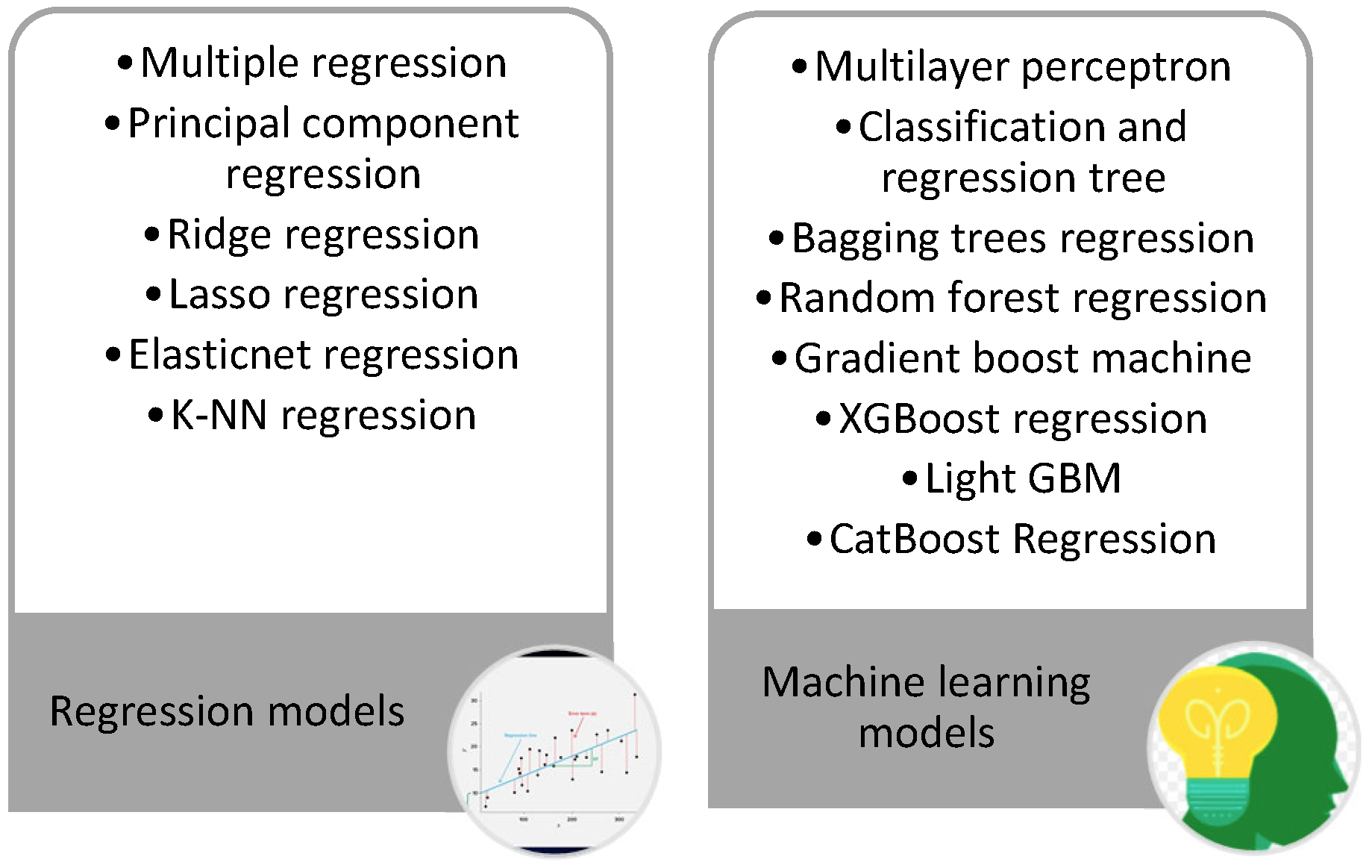
There are many studies carried out using machine learning and regression models in the field of forecasting, as shown in Table 2. In this study, the methods used in machine learning and regression model are multiple regression, principle component regression, ridge regression, lasso regression, elastic net regression, K-nearest neighbor, multilayer perceptron, bagging trees, random forest, gradient boost machine, XGboost algorithm, and CatBoost algorithm.
Arslan and Ertuğrul [15] analyzed the electricity price and compared the performance of multiple regression models and artificial neural network models.
Fumo and Biswas [16] performed a simple and multiple linear regression model along with a quadratic regression analysis. Multiple linear regression models using outdoor temperature and solar radiation offered an improved coefficient of determination.
Jang et al. [17] focused on the effects of geological parameters to the overbreak phenomenon by applying linear and nonlinear multiple regression and artificial neural networks (ANNs). The performance of these algorithms was evaluated by comparing correlations.
Nguyen and Cripps [18] compared the performance of two method called artificial neural network and multiple regression analysis for predicting house sales. Artificial neural network solutions are better than multiple regression analysis solutions.
Talaat and Gamel [19] examined the effects of co-author count on the number of citations using Pearson’s correlation coefficient and multiple linear regression. They compared the correlations between number of authors, number of countries, citation count, venue category, and year-from.
Sun et al. [20] used the random forest algorithm to predict the research octane number of gasoline. They indicated that the properties of gasoline effect the research octane number of gasoline, and complex relations can be modeled by using a random forest algorithm.
Adami et al. [21] introduced the clinical and bone metabolic risk factors using principal component analysis (PCA) and principal component regression (PCR). They found that some factors such as age, GC treatment, ACPA titer, etc. were negatively affected.
Yan et al. [22] compared different regression methods such as principal component regression and partial least squares regression for analyzing flight load. Then they demonstrate the efficiency and capabilities of these methods.
Effendi et al. [23] used principal component regression to predict the farmer exchange rate. Their analysis showed that harvest area, production, and the human development index affect the farmer exchange rate.
Sing et al. [24] compared principal component regression and partial least squares regression methods for estimating the piperine content in black pepper. The efficiency of these methods was evaluated by root mean square error and correlation coefficient.
Tahir and Ilyas [25] compared the result of the robust correlation-based regression and robust correlation scaled principal regression. Also, they proposed a model called as macro robust correlation scaled principal component regression, which can deal with missing values, cellwise outliers, row-wise outliers, high dimensions, and multicollinearity.
Lettink et al. [26] investigated the two-dimensional fused ridge estimator of the linear and logistic regression models. Then they developed an implementation of the cross-validation method. They showed the use of this method to predict health indicators.
Zandi et al. [27] used a locally weighted linear regression method for evaluating the potential of three large-scale products. They also used the L2 regularization for overcoming the multicollinearity problem.
Zhang et al. [28] introduced an algorithm which reduced the subspace and obtained optimal statistical machine learnings models. For simplicity, the polynomial ridge regression (RR) algorithm was used to learn the norm and Hamiltonian kernels of axially deformed configurations.
Zheng et al. [29] predicted wind speed using kernel ridge regression and then compared the results using methods such as support vector machine (SVM) and artificial neural networks (ANNs). The root means square error (RMSE) and root mean square (R2) were used to calculate the effectiveness of these algorithms.
Song et al. [30] proposed a model based on lasso regression to improve the applicability and effectivity of the model. They predicted the mine face gas concentration. After that, they compared the model with a long short-term memory prediction model.
Li et al. [31] combined a forecasting model using lasso regression and optimal integration. Also, ARIMA, NARNN, LSTM, and 11 other single forecasting models were used in their study.
Sharma et al. [32] compared compressive strength by using linear regression, lasso regression, and ridge regression. Some statistical measurements such as MSE, MAE, and RMSE were evaluated to calculate the performance of the methods.
Didari et al. [33] selected variables for predicting dryland wheat yield by using lasso regression. The result is that the lasso regression could be used reliably for each district considering the most effective meteorological parameters.
Malakouti [34] predicted the amount of carbon dioxide used by elastic net and lasso algorithms. After that, the methods were compared with the mean square error, mean absolute error, root mean square error, and mean absolute percentage error.
The originality of this study lies in its integration of statistical regression and advanced machine learning models in a single framework, with a specific focus on the role of meteorological variables in urban travel time prediction. Unlike previous studies, which often neglected environmental factors or focused solely on model performance, this research provides a systematic analysis of weather impacts and model sensitivity. Therefore, it contributes not only to methodological improvement but also to the practical deployment of smart transportation infrastructure.

4. Methods and Applications

The framework of the study is given in Figure 1. The study is divided into five phases: data collecting, data preprocessing, modeling, model evaluation, and model selection. A detailed description of each phase is presented in this section.

4.1. Data Collecting

This stage is the first stage of the study, where the data is obtained. It can be described as the stage in which it is decided which characteristics the obtained data should have. In the study, the data of a city bus line belonging to a public transportation company operating in Turkey were used.
According to interviews with transportation company officials and experts, route number “R049 Organize Sanayi RSİ-Hörmetçi Aktarma” was deemed appropriate to carry out the works. The selected R049 route represents one of the longest and most frequently used lines in the Kayseri public transport network, connecting residential zones with the Organized Industrial Area. This route was chosen because it captures diverse traffic and meteorological conditions—ranging from urban congestion near the city center to open-road segments in suburban areas—thus offering representative variability for model training.
The study period (November 2021–July 2022) was deliberately selected to include both winter and summer months, allowing the analysis to capture the seasonal influence of weather conditions on travel time. Although the dataset is limited to a single route, it reflects operational and environmental heterogeneity typical of mid-sized Turkish cities, providing a meaningful foundation for generalization to similar contexts. The route map along with the bus-stop location is shown in Figure 2.
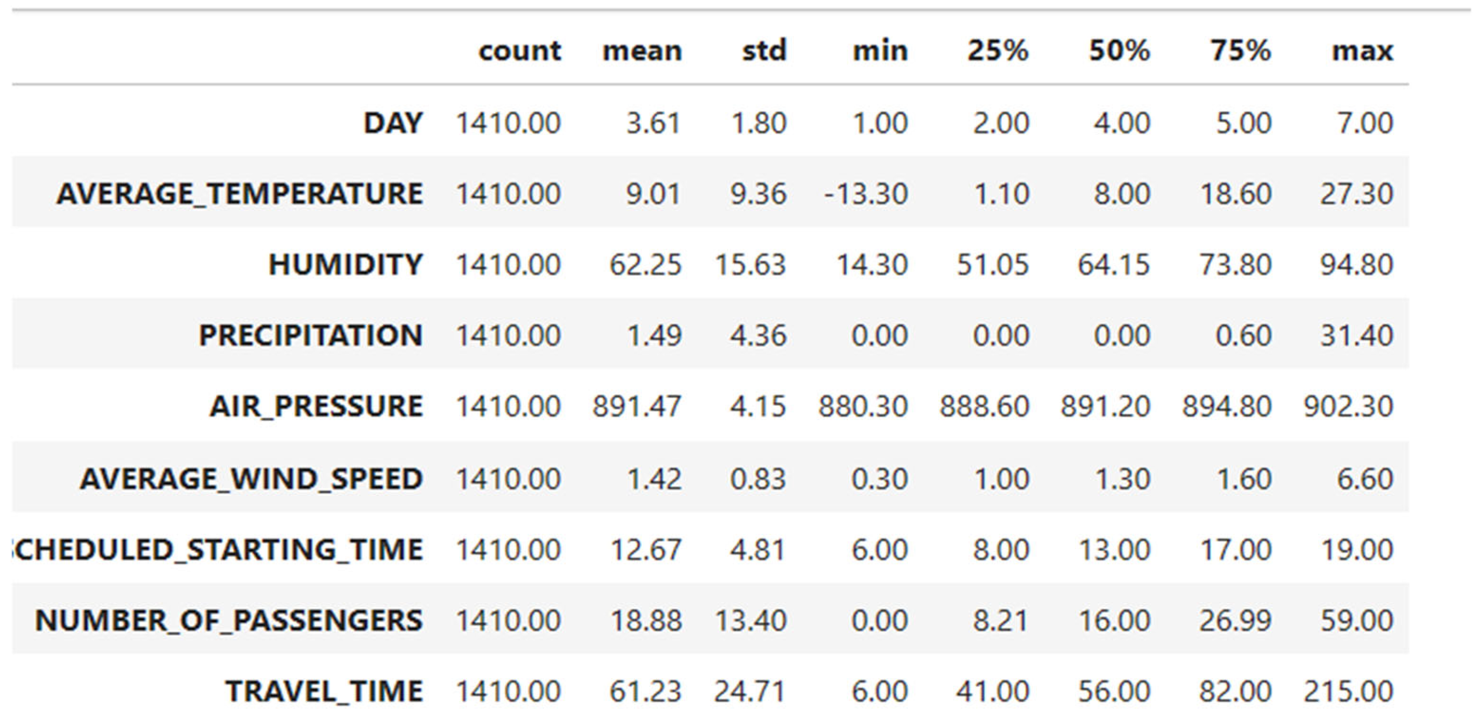
In order to examine the effects of weather conditions on bus services, weather conditions of the period in question were also collected. Data between 5 November 2021 and 28 July 2022 are used in the study. A total of 1410 trips were observed for the specified time period. Meteorological data were retrieved from the Turkish State Meteorological Service (MGM) and synchronized with each bus trip according to its date and scheduled departure time. For each record, daily averages of temperature, humidity, air pressure, wind speed, and total daily precipitation were used to represent the environmental conditions during the corresponding day. In the study, we tried to predict the values that the travel time variable will take depending on the day, average temperature, humidity, precipitation, air pressure, average wind speed, scheduled starting time, and number of passengers variables.
The variables and definitions are as shown in Table 3.
A snapshot of the data collected is given in Figure 3.
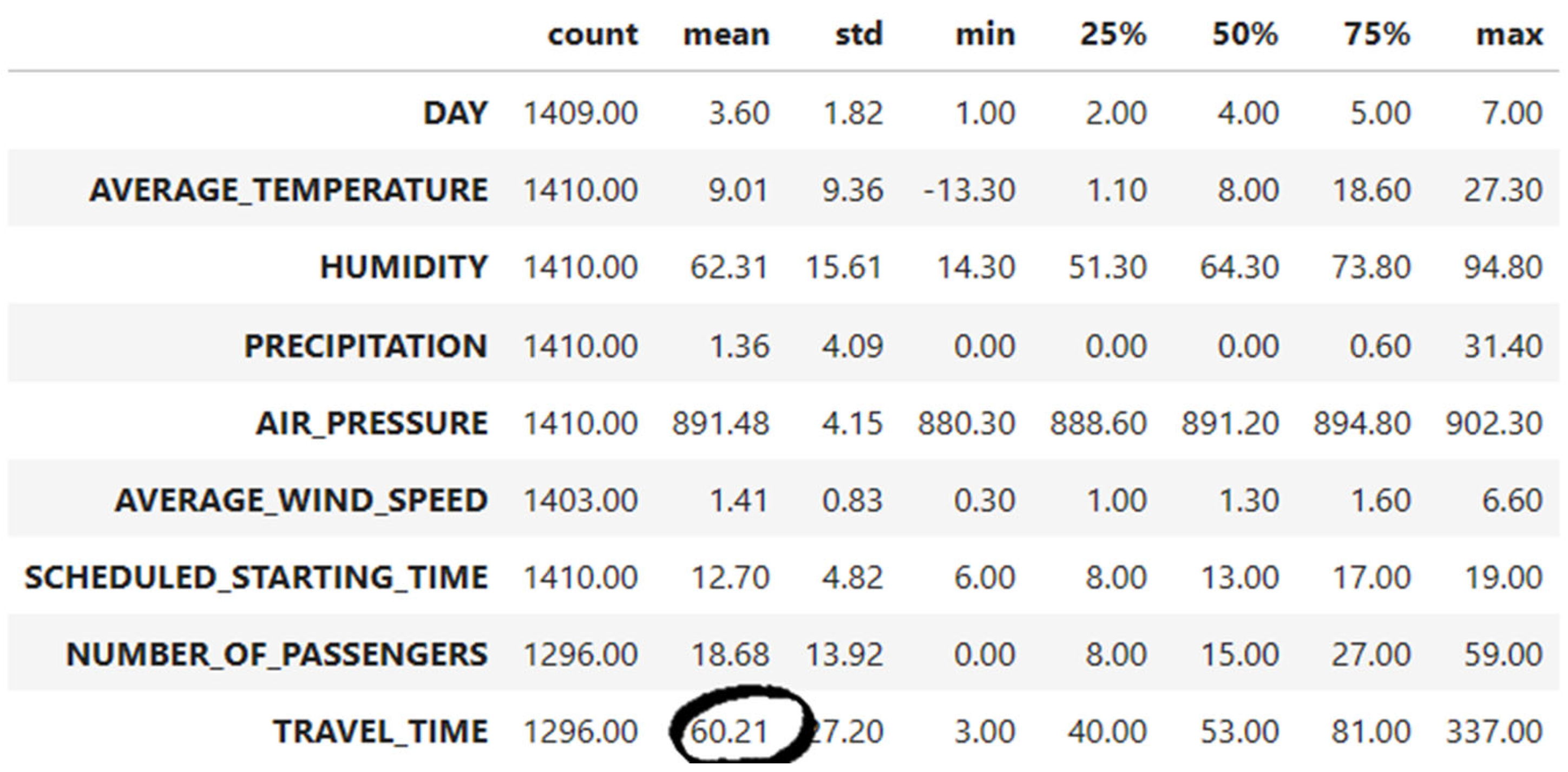
For transportation companies, it is important that the travel times are estimated correctly, and the planning is carried out according to these estimations. The transportation company stated that the travel time should be 45 min. However, as shown in Figure 4, in practice, travel time was found to be 60.21 min.
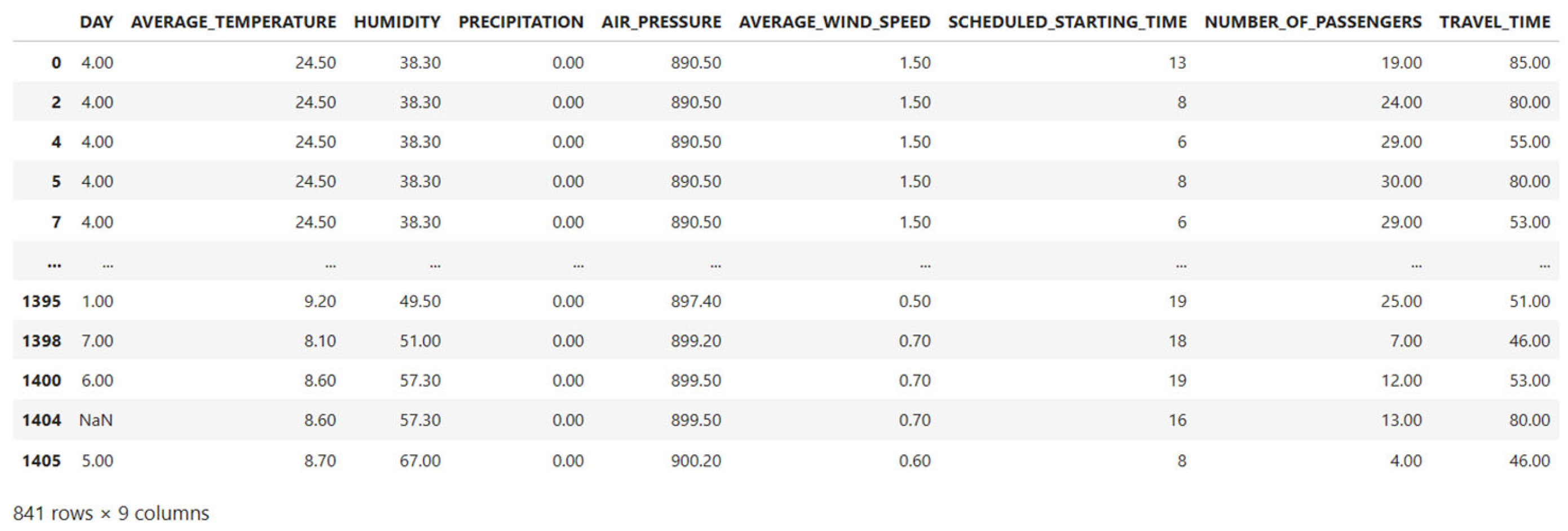
In addition, there were 841 observations that exceeded the standard travel time determined by the transportation company. The examples of these observations are shown in Figure 5.

4.2. Data Preprocessing

The data of the observations obtained must be preprocessed before being used in any regression model or machine learning algorithm. Thus, more meaningful results can be obtained by removing noisy, erroneous, and redundant data from the dataset [7]. The data preprocessing phases carried out are as shown in Figure 6.
Missing values occur when no data value is stored for the variable in an observation. Missing values have a significant effect on the conclusions. For this reason, researchers must try to eliminate this problem. Many approaches are available to tackle the problems imposed by missing values in data preprocessing. For example, the instances which have missing values can be discarded; can be assigned a value such as mean or mode; or can be obtained by using a prediction method like KNN, random forest, etc. [34].
Outliers are patterns in data that do not conform to a well-defined notion of normal behavior [35]. While it is easy to identify outliers in datasets with a single variable, it is more difficult in datasets with multiple variables. For this reason, researchers have developed different methods. The local outlier factor (LOF) method is one of these methods. The basic idea of the LOF is to define the degree of an outlier of the point by assigning an object’s deviation factor in the dataset.
By applying these steps, data is prepared for analysis. The travel time was the dependent variable and day, average temperature, humidity, precipitation, air pressure, average wind speed, scheduled starting time, and number of passengers were the independent variables.
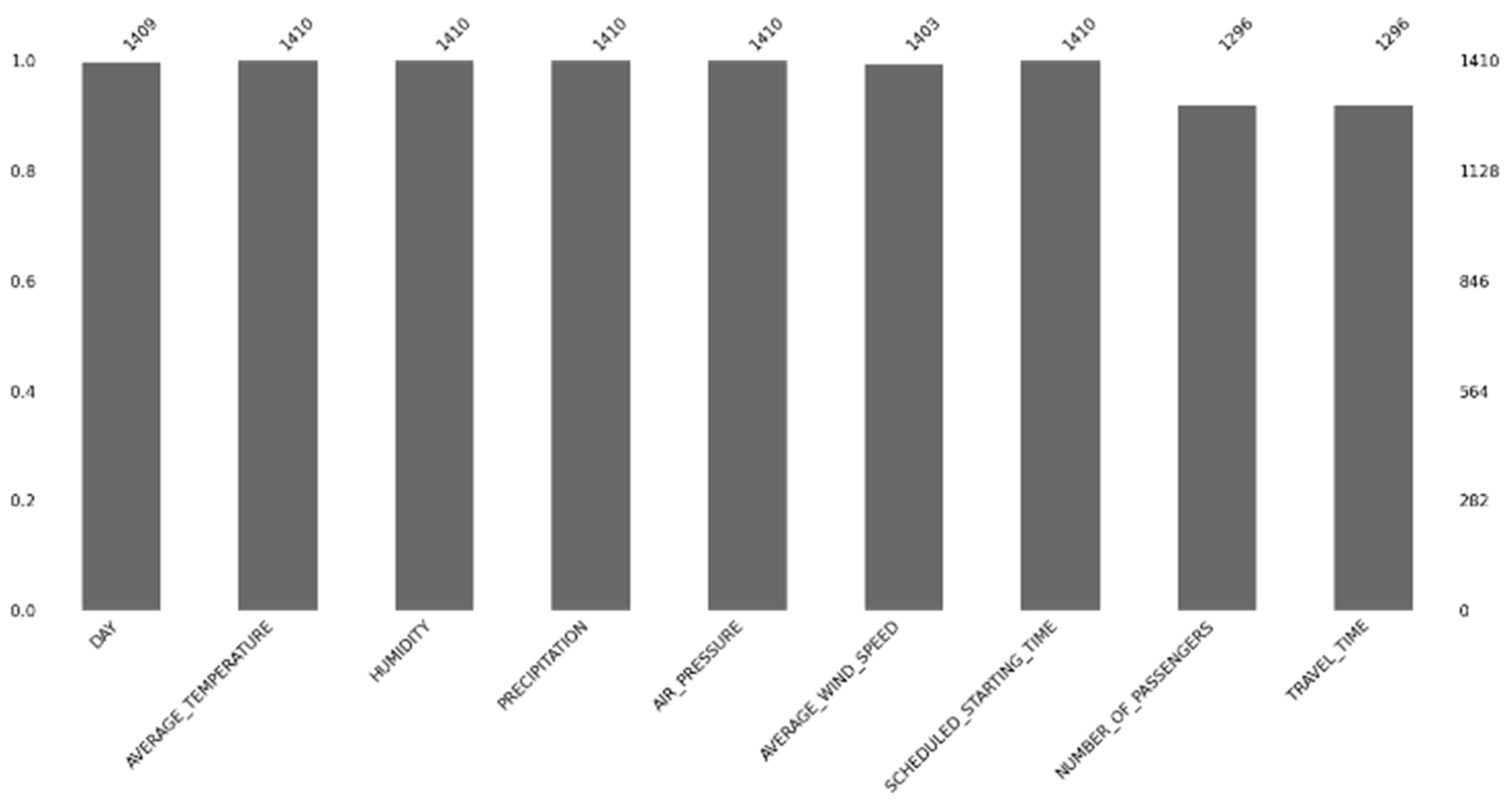
Firstly, the missing values in the dataset were obtained for each variable. The bar chart is as shown in Figure 7.
Then the instances which had missing values were assigned a value obtained by using a prediction method which is called KNN. The k value, which is the model parameter, was accepted as 4. The missing values were completed according to the estimated values with this algorithm. The old data and the new data obtained by using the KNN method are shown in Figure 8 and Figure 9.
A preliminary analysis was conducted to understand the correlation between the independent variables and the dependent variables. A heat map using the seaborn library in Python 3.10 (Python Software Foundation, Wilmington, DE, USA) is shown in Figure 10.
A heat map depicts values for a main variable of interest across two axis variables as a grid of colored squares. According to Figure 10, there is a very low correlation between almost all variables. However, the observed perfect correlation (1.0) between number_of_passengers and travel_time suggests a potential data leakage issue. This may indicate that the passenger count is either directly derived from or strongly collinear with the actual travel time. Although this variable was retained for analysis due to its operational relevance, future studies should investigate its causal direction and consider alternative feature engineering strategies to mitigate overfitting risks.
In this study, one of the most prevalent outlier detection algorithms, LOF, was used. In order to apply this method, density values were calculated for each data point using the KNN algorithm. The data were sorted according to these density values, and the outliers were converted to the threshold value according to the order. Accordingly, 14 outliers were found in the dataset, as shown in Figure 11. In this context, each observation was assigned a local density score based on the local outlier factor (LOF) method. The data points were then sorted in ascending order of their density values, and those below the 13th-ranked density were defined as outliers. Therefore, the phrase “threshold = 13th data” indicates that the 13th lowest density value was used as the cutoff for outlier detection.
The threshold value obtained is as shown in Figure 12.
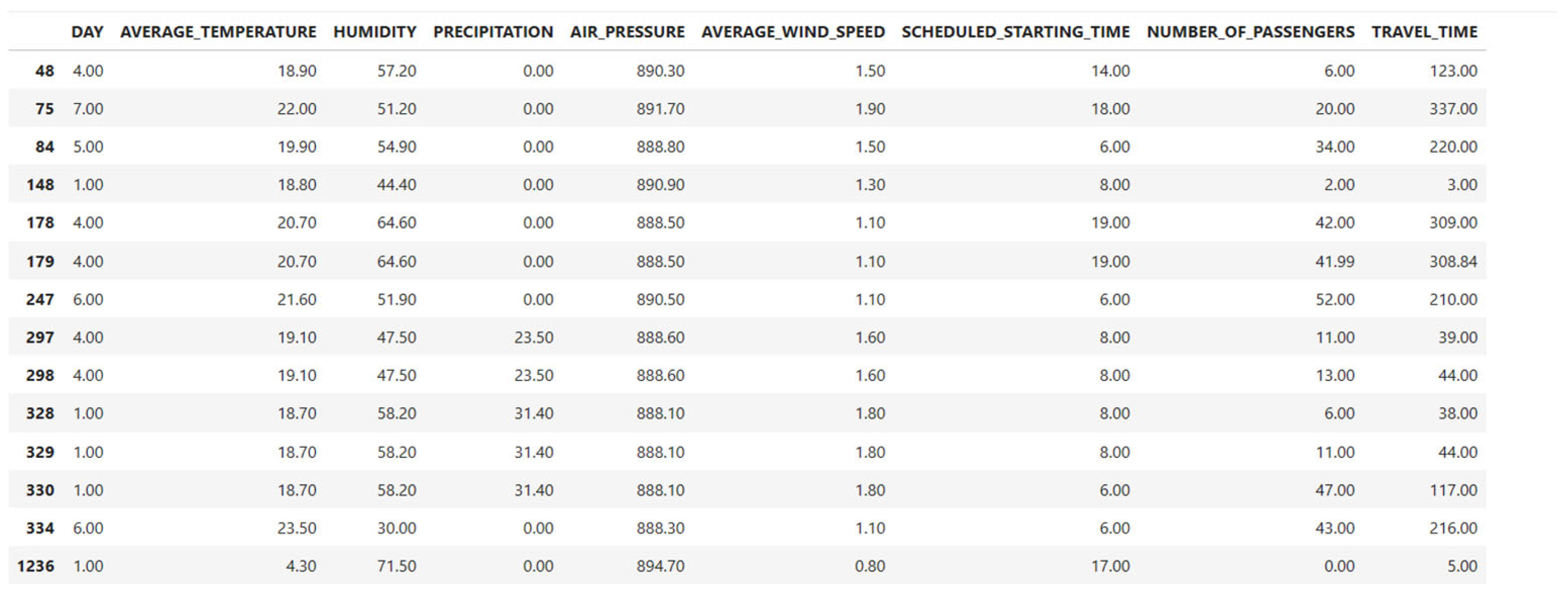
These 14 observations had the following data and were replaced by the threshold value. The outliers are as shown in Figure 13.
After the preprocessing phase, the information in the dataset is as shown in Figure 14.

4.3. Modeling

The travel time prediction was obtained by using regression models and machine learning models for the selected route, such as multiple linear regression (MLR), principal component regression (PCR), ridge regression, lasso regression, elastic net regression, K-nearest neighbors, multilayer perceptron (MLP), classification and regression tree (CART), bagging trees regression, random forest regression, gradient boost machine (GBM), light GBM, and XGboost regression, as shown in Figure 15.
Since each bus trip is an independent record rather than a continuous time series, recurrent and sequential neural network architectures such as LSTM or GRU were not applicable to this dataset.

4.3.1. Regression Models

Regression analysis is a methodology that allows for finding a functional relationship among response or dependent variables and predictor, explanatory, or independent variables. For complex systems, the regression analysis should be viewed as an iterative process [16]. The regression models used in this study are described below.
Multiple Linear Regression (MLR)
Multiple linear regression is the generalization of the simple linear regression model. The model in multiple linear regression allows for more than one predictor variable.
Y   =   0 + 1 X 1 + 2 X 2 + + p X p +
where Y is the response variable; X 1 , X 2 , , X p are the predictor variables with p as the number of variables; 0 , 1 , , p are the regression coefficients; and is an error to account for the gap between predicted data and observed data.
Principal Component Regression (PCR)
Principal component regression is a basic, but very powerful, multivariate calibration method. When discussing multivariate analysis techniques, including PCR, three terms are often used: variance, vector, and projection. The term “vector” is used to describe a line segment in a coordinate system with a specific direction, and the term “projection” is used to describe the distance of a point along a vector.
Ridge Regression
Ridge regression is a popular parameter estimation method used to address collinearity problems frequently arising in multiple linear regression. The aim is to find the coefficients that minimize the mean absolute error by applying a penalty to the coefficients. It uses the L 2 approach as shown in Equation (2).
S S E L 2 = i = 1 n y i y ^ i 2 + λ j = 1 P β j 2
where λ is the setting parameter and j = 1 P β j 2 is the penalty term.
The λ   parameter is important, so the cross-validation method is used to find a good value.
Lasso Regression
The lasso is a method for regularizing a least squares regression. Suppose we have predictor measurements x i j , j = 1,2 , , p and an outcome measurement y i , observed for cases i = 1,2 , . , N . The lasso fits a linear regression model by solving the optimization problem
min β i = 1 N y i β 0 j = 1 p x i j β j 2  
subject to
j = 1 p β j s [36].
Ridge and lasso regression are not superior to each other. It uses the L 1 approach as shown in Equation (3).
Elastic Net Regression
The elastic net regression is a form of regularized optimization for linear regression that provides a bridge between ridge regression and the lasso [37]. It uses both the L 1 approach and L 2 approach as shown in Equation (4).
S S E E n e t = i = 1 n y i y ^ i 2 + λ 1 j = 1 P β j 2 + λ 2 j = 1 P β j
K-Nearest Neighbors
The K-nearest neighbor (KNN) method has widely been used in the applications of data mining and machine learning due to its simple implementation and distinguished performance [38]. KNN regression is also known as a lazy learner; it is a basic non-linear model which works on the principle of similarity [7]. KNN methods are as shown [39]:
  • Assigning an optimal k value with a fixed expert predefined value for all test samples.
  • Assigning different optimal k values for different test samples.

4.3.2. Machine Learning Models

Machine learning (ML) is the scientific area of algorithms and statistical models that computer systems use to execute a specific duty without being explicitly programmed. In recent years, researchers have used machine learning methods in many areas. The machine learning models used in this study are described below.
Multilayer Perceptron (MLP)
Multilayer perceptron neural network models are a type of artificial neural network that use nonlinear functions. These models consist of three types: the input layer, the hidden layer(s), and the output layer. The input layer receives the input signals. There are weights connecting the input and hidden layers and weights connecting the hidden layers and output layer. Multilayer perceptron learns and makes predictions using these components [40].
Classification And Regression Tree (CART)
Classification and regression tree algorithms extract decision rules from features, which may include either numerical or categorical values, and builds a model to predict the target values [41]. CART produces the most explicit information compared to other machine learning algorithms [42].
CART algorithms include four basic steps; in the first step, a tree is built using recursive splitting of nodes. Each node is assigned to a class. In the second step, a maximal tree is produced and obtains information using the learning dataset. The next step consists of tree “pruning”, and the last step consists of optimal tree selection [43].
Bagging Trees Regression
A bagging tree chooses several subsets of data randomly with replacement from the training sample [44]. This tree is also known as bootstrap aggregation. When compared to boosting technique, a bagging tree has advantages of minimizing the decision tree training error. The aim is to reduce the variance of the predictor and avoid overfitting.
Random Forest Regression
Random forest regression is a machine learning model which is developed with the intention of modeling the output variables according to the inputs. This regression model is aimed at predicting the structure of each tree and computing to utilize the training dataset. In this model, a lot of decision trees are obtained and tested [45].
Gradient Boost Machine, Light GBM, and XGBoost Regression
The gradient boost algorithm utilizes an ensemble, which is used to simplistically eliminate bias, noise, and variance, which dilute the effectiveness of the prediction model. The ensemble employs bagging and boosting techniques, which pre-build many independent models and which is tested and then implemented sequentially to allow the new models to learn from the mistakes of the previous models [46].
In machine learning algorithms, the light gradient boosting machine model is a more efficient ensemble learning model than other existing ensemble learning models. The performance of this algorithm is related to selecting the hyper parameter configuration. Thus, the hyper parameters must be chosen correctly. The hyperparameter choosing algorithms are grid search (Grid), random search, covariance matrix adaptive evolution strategy, and the tree-structured Parzen estimator [47].
An extreme gradient boost algorithm is a flexible model, and its hyperparameters can be tuned using soft computer algorithms. Thus, it is more accurate and faster than the other algorithms. In every step, the loss function can be reduced using the residual of the previous tree [48].

4.3.3. The Applications of Algorithms in Prediction the Travel Time

For all machine learning algorithms, hyperparameter optimization was performed using a grid search method with K-fold cross-validation (k = 5). The hyperparameters tuned for each algorithm included the learning rate, maximum depth, the number of estimators for ensemble models (e.g., CatBoost, XGBoost), and the number of neurons and layers for neural networks. The best-performing parameters were selected based on the lowest mean squared error (MSE) on validation folds.
Feature importance was calculated for tree-based models using built-in importance metrics. In CatBoost, the most influential variables were number_of_passengers, scheduled_starting_time, and precipitation. This analysis highlights the role of weather-related parameters in travel time prediction. The travel time prediction was obtained by using the regression models and machine learning models for the selected route, such as multiple linear regression (MLR), principal component regression (PCR), ridge regression, lasso regression, elastic net regression, K-nearest neighbors, multilayer perceptron (MLP), classification and regression tree (CART), bagging trees regression, random forest regression, gradient boost machine (GBM), light GBM, and XGboost regression.
In this study, the hybrid modeling framework was implemented in two complementary stages. In the first stage, statistical regression models (MLR, PCR, ridge, lasso, and elastic net) were employed to establish baseline relationships and identify the relative influence of each explanatory variable. These models provide interpretable coefficients and assist in detecting multicollinearity or redundancy among predictors. In the second stage, machine learning algorithms (e.g., random forest, gradient boosting, XGBoost, CatBoost, and MLP) were trained on the same standardized dataset to capture nonlinear and interaction effects that cannot be represented by traditional regressions. The comparative evaluation of these two model groups formed the basis of the proposed hybrid framework, allowing both interpretability and high predictive performance to be jointly assessed.
In order to produce predictions with machine learning methods, it is necessary to divide the data into training and test data. There are various methods in the literature for this process. In this study, separation of training and test data was performed with the K-fold cross-validation method. The data were divided into training and test datasets with a 0.75/0.25 split. The algorithm that gave the best results was obtained, and then, sensitivity analyses were carried out by changing various parameters.
The model tuning phase was also performed to find the optimal values of hyperparameters to maximize model performance. Hyperparameters in the machine learning algorithms are the set of variables whose values cannot be estimated by the model from the training data. Thus, model tuning can be called hyperparameter optimization. Thanks to model tuning, different hyperparameter values were obtained for each algorithm, and the options that gave the best results were obtained by using these hyperparameter values.
The main hyperparameters used for each algorithm are summarized as follows:
-
KNN: k = 4–8;
-
Random forest: n_estimators = 200, max_depth = 10;
-
XGBoost: learning_rate = 0.1, n_estimators = 300, max_depth = 8;
-
CatBoost: learning_rate = 0.05, depth = 8, iterations = 500;
-
MLP: hidden_layer_sizes = (50, 25), activation = ‘relu’, solver = ‘adam’.
All models were optimized using a grid search with 5-fold cross-validation.

4.4. Modeling Evaluation and Model Selection

In the study, in addition to model tuning, sensitivity analyses were also carried out according to the change in the k value in the KNN algorithm and the change in the threshold values used to determine outliers.
Analysis 1: The Change in the Threshold Values Used to Determine Outliers.
According to the change in the threshold value used to determine the outliers, the mean squared error values of each algorithm are as seen in Figure 16. In this situation, the instances which had missing values were assigned a value obtained by using a prediction method called KNN, where the k value was accepted as 4.
As seen in Figure 16, according to algorithms, the results are similar to each other. The values of each algorithm are shown in Table 4.
As shown in Table 4, nearly all of the minimum error values were obtained by using the CatBoost algorithm. Also, the minimum error values of each algorithm were obtained when the threshold value was 100.
According to the change in the threshold value in determining the outliers, the mean squared error values of each algorithm are as seen in Figure 17. In this situation, the instances which had missing values were assigned a value obtained by using a prediction method called KNN, where the k value was accepted as 5.
As seen in Figure 17, according to the algorithms, the results are similar to each other. The values for each algorithm are shown in Table 5.
As shown in Table 5, nearly all of the minimum error values were obtained by using the CatBoost algorithm. Also, nearly all of the minimum error values of each algorithm were obtained when the threshold value was 100.
Analysis 2: The Change in the K Value in the KNN Algorithm.
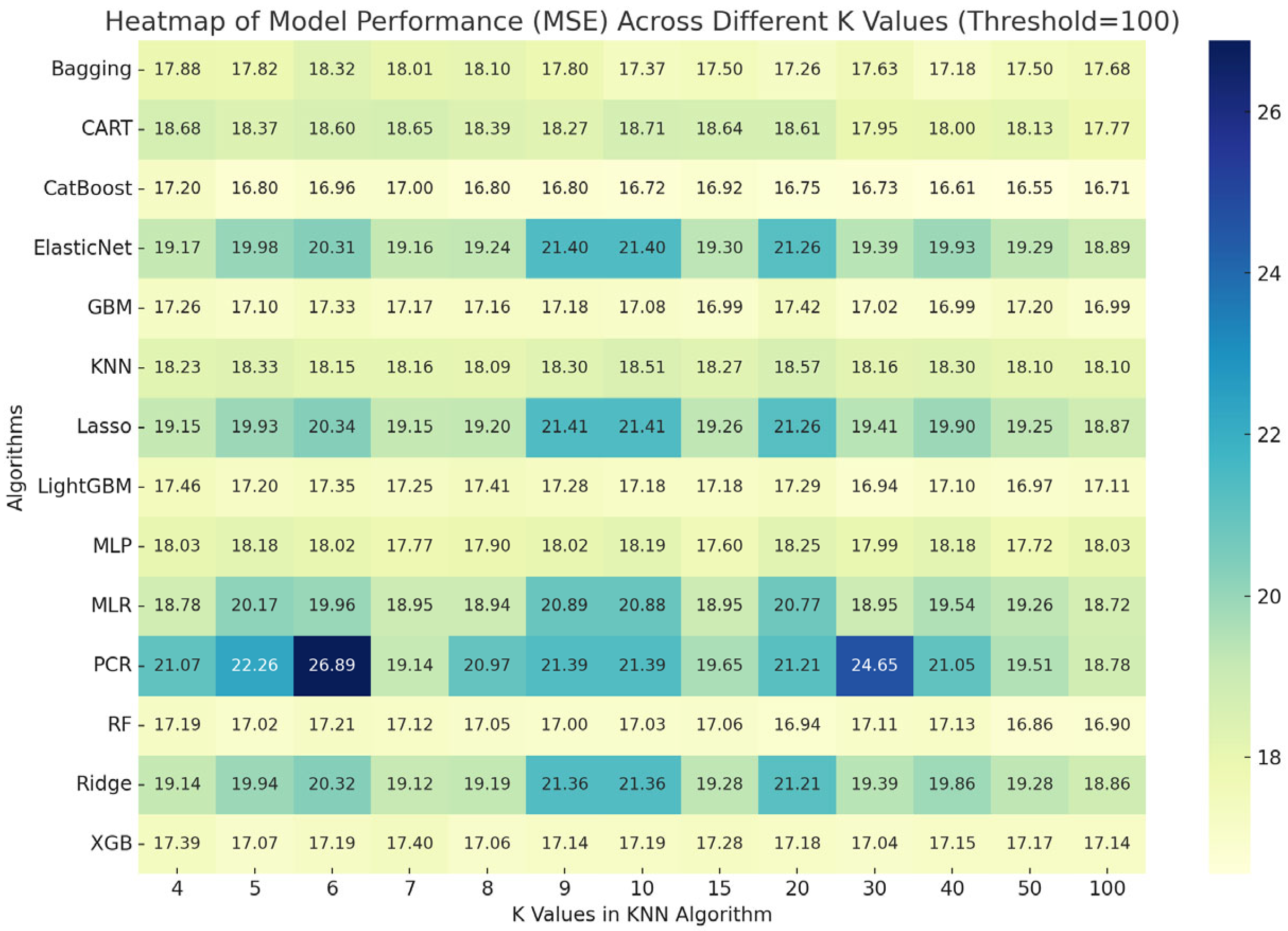
Thus, while the threshold values were constant, the error values were analyzed according to the change in the k values. The results are as shown in Table 6.
As illustrated in Table 6 and Figure 18, the CatBoost algorithm consistently produced the lowest mean squared error (MSE) values across all parameter settings. This superior performance indicates that gradient boosting-based approaches, particularly CatBoost, exhibited higher robustness and generalization capability compared to other regression and machine learning models under varying preprocessing conditions.
To statistically validate these performance differences, a Friedman test was conducted based on the MSE values of all algorithms. The test results as shown in Table 7 confirmed that the differences among the models were statistically significant (χ2 = 148.54, df = 12, p < 0.001), rejecting the null hypothesis of equal treatment effects. The test was conducted at a 95% confidence level.
Considering the values as shown in Table 6, the CatBoost algorithm achieved the lowest median error value among all models. Therefore, it was selected as the reference model in the Wilcoxon signed-rank test. The test results (p = 0.002 for all comparisons) confirmed that CatBoost performed statistically better than the other algorithms.

5. Conclusions

This study investigates the impact of weather conditions on public bus travel times using both traditional regression and modern machine learning algorithms. Unlike prior studies, it combines statistical and machine learning techniques in a unified framework while incorporating weather variables often overlooked in the literature.
The analysis reveals that the CatBoost algorithm consistently yielded the lowest mean squared error across different preprocessing scenarios, including variations in KNN k values and outlier threshold settings. The inclusion of meteorological variables yielded significant improvements in model performance. These results underline the predictive power of environmental features in urban transportation modeling. Conceptually, these findings support a causal framework where meteorological factors act as exogenous drivers of variability in travel time through both mechanical (e.g., road friction, engine load) and behavioral (e.g., driver caution, passenger flow) pathways. This aligns with transport system resilience theory, which emphasizes the sensitivity of urban mobility performance to environmental disturbances. Thus, the inclusion of weather parameters not only enhances predictive accuracy but also enriches the explanatory depth of the model. Additionally, the robustness of the proposed approach was validated through sensitivity analyses, where CatBoost maintained superior accuracy across varying k-values and outlier thresholds. This suggests that gradient boosting-based models are more resilient to noise and variability in transport-related data.
To further validate these findings, non-parametric statistical analyses were conducted. The Friedman test confirmed that the performance differences among algorithms were statistically significant (χ2 = 148.54, df = 12, p < 0.001), rejecting the null hypothesis of equal treatment effects. Following this, pairwise Wilcoxon signed-rank tests (p = 0.002 for all comparisons) revealed that CatBoost significantly outperformed the other algorithms. These statistical results substantiate the robustness of the proposed approach and strengthen the conclusion that CatBoost offers the most reliable performance for travel time prediction under varying preprocessing and parameter settings.
The hybrid modeling strategy adopted in this study bridges the interpretability of regression-based models with the predictive flexibility of machine learning algorithms, offering a balanced and transparent framework for travel time estimation.
Beyond the empirical improvement in predictive performance, the study also provides a theoretical contribution by clarifying how meteorological variability systematically influences travel time dynamics through physical, operational, and behavioral mechanisms.
The selected R049 route was intentionally used because it connects industrial and residential regions under varying meteorological conditions and traffic densities, offering a representative testbed for the proposed modeling framework.
However, a critical limitation is the relatively small dataset (N = 1410), which corresponds to a single bus route observed over a nine-month period. Although the dataset size was sufficient for cross-validation and sensitivity analyses across multiple algorithms, future research should employ larger, multi-route datasets to enhance robustness and generalizability.
From a practical standpoint, the developed framework can guide transport authorities in designing data-driven scheduling and monitoring systems. By integrating such predictive models into real-time control centers, transit agencies could dynamically adjust route frequencies or provide accurate arrival information to passengers under varying weather conditions. These applications would enhance service reliability and support sustainable urban mobility policies.
Future research should expand the dataset over multiple cities and seasons, incorporate real-time traffic data, and apply more advanced time-series models such as LSTM or Transformer architectures. In addition, feature importance analyses and SHAP-based interpretability tools could be used to uncover the relative influence of each weather parameter. These improvements would contribute to the development of robust, real-time, and adaptive public transport management systems.
In this study, the performance of regression and machine learning algorithms were analyzed. In addition to this study, not only for the k values and threshold values but also the different parameter values of each algorithm, sensitivity analyses were performed. Thus, we aimed to achieve lower error values.

Funding

This research received no external funding.

Institutional Review Board Statement

Not applicable.

Informed Consent Statement

Not applicable.

Data Availability Statement

The data presented in this study are available in the article.

Conflicts of Interest

The author declares no conflicts of interest.

Abbreviations

The following abbreviations are used in this manuscript:
ANNArtificial Neural Network
ARIMAAuto-Regressive Integrated Moving Average
CARTClassification and Regression Tree
GBMGradient Boosting Machine
KNNK-Nearest Neighbors
LOFLocal Outlier Factor
LSTMLong Short-Term Memory
MAEMean Absolute Error
MLMachine Learning
MLPMultilayer Perceptron
MLRMultiple Linear Regression
MSEMean Squared Error
PCRPrincipal Component Regression
RMSERoot Mean Square Error
SVRSupport Vector Regression
XGBoostExtreme Gradient Boosting

References

  1. Serin, F.; Alisan, Y.; Erturkler, M. Predicting bus travel time using machine learning methods with three-layer architecture. Measurement 2022, 198, 111403. [Google Scholar] [CrossRef]
  2. Gal, A.; Mandelbaum, A.; Schnitzler, F.; Senderovich, A.; Weidlich, M. Traveling time prediction in scheduled transportation with journey segments. Inf. Syst. 2017, 64, 266–280. [Google Scholar] [CrossRef]
  3. Peterson, N.C.; Rodrigues, F.; Pereira, F.C. Multi-output bus travel time prediction with convolutional LSTM neural network. Expert Syst. Appl. 2019, 120, 426–435. [Google Scholar] [CrossRef]
  4. Bai, C.; Peng, Z.R.; Lu, Q.C.; Sun, J. Dynamic bus travel time prediction models on roaad with multiple bus routes. Comput. Intell. Neurosci. 2015, 2015, 1–10. [Google Scholar] [CrossRef]
  5. Treethidtaphat, W.; Atikom, W.P.; Khaimook, S. Bus Arrival Time Prediction at Any Distance of Bus Route Using Deep Neural Network Model. In Proceedings of the IEEE 20th International Conference on Intelligent Transportation Systems (ITSC): Workshop, Yokohama, Japan, 16–19 October 2017; pp. 757–762. [Google Scholar] [CrossRef]
  6. Chen, M.Y.; Chiang, H.S.; Yang, K.J. Constructing cooperative intelligent transport systems for travel time prediction with deep learning approaches. IEEE Trans. Intell. Transp. Syst. 2022, 23, 16590–16599. [Google Scholar] [CrossRef]
  7. Ashwini, B.P.; Sumathi, R.; Sudhira, H.S. Bus Travel Time Prediction: A Comparative Study of Linear and Non-Linear Machine Learning Models. J. Phys. Conf. Ser. 2022, 2161, 012053. [Google Scholar] [CrossRef]
  8. Servos, N.; Liu, X.; Teucke, M.; Freitag, F. Travel Time Prediction in a Multimodal Freight Travel Time Prediction in a Multimodal Freight Learning Algorithms. Logistics 2020, 4, 1. [Google Scholar] [CrossRef]
  9. Ceylan, H.; Özcan, T. Optimization of Service Frequencies in Bus Networks with Harmony Search Algorithm: An Application on Mandl's Tet Network. Pamukkale Univ. J. Eng. Sci. 2018, 24, 1107–1116. [Google Scholar] [CrossRef]
  10. Reddy, K.K.; Kumar, B.; Vanajakshi, L. Bus travel time prediction under high variability conditions. Curr. Sci. 2016, 111, 700–711. [Google Scholar] [CrossRef]
  11. Mossavi, S.M.H.; Aghaabbasi, M.; Yuen, C.W. Evaluation of Applicability and Accuracy of Bus Travel Time Prediction in High and Low Frequency Bus Routes Using Tree-Based ML Techniques. J. Soft Comput. Civ. Eng. 2023, 7, 74–97. [Google Scholar]
  12. Wu, J.; Wu, Q.; Cai, C. Towards Attention-Based Convolutional Long Short-Term Memory for Travel Time Prediction of Bus Journeys. Sensors 2020, 20, 3354. [Google Scholar] [CrossRef] [PubMed]
  13. Lee, G.; Choo, S.; Choi, S.; Lee, H. Does the Inclusion of Spatio-Temporal Feature Improve Bus Travel Time Predictions? A Deep Learning-Based Modelling Approach. Sustainability 2022, 14, 7431. [Google Scholar] [CrossRef]
  14. He, P.; Jiang, G.; Lam, S.K.; Tang, D. Travel-Time Prediction of Bus Journey with Multiple Bus Trips. IEEE Trans. Intell. Transp. Syst. 2019, 20, 4192–4205. [Google Scholar] [CrossRef]
  15. Arslan, B.; Ertuğrul, İ. Çoklu Regresyon, ARIMA ve Yapay Sinir Ağı Yöntemleri ile Türkiye Elektrik Piyasasında Fiyat Tahmin ve Analizi. Yönetim Ve Ekon. Araştırmaları Derg. 2022, 20, 331–353. [Google Scholar] [CrossRef]
  16. Fumo, N.; Biswas, M. Regression analysis for prediction of residential energy consumption. Renew. Sustain. Energy Rev. 2015, 47, 332–343. [Google Scholar] [CrossRef]
  17. Jang, H.; Topal, E. Optimizing overbreak prediction based on geological parameters comparing multiple regression analysis and artificial neural network. Tunn. Undergr. Space Technol. 2013, 38, 161–169. [Google Scholar] [CrossRef]
  18. Nguyen, N.; Cripps, A. Predicting Housing Value: A Comparison of Multiple Regression Analysis and Artificial Neural Networks. J. Real Estate Res. 2021, 22, 313–336. [Google Scholar] [CrossRef]
  19. Talaat, F.M.; Gamel, S.A. Predicting the impact of no. of authors on no. of citations of research publications based on neural networks. J. Ambient Intell. Humaniz. Comput. 2022, 14, 8499–8509. [Google Scholar] [CrossRef]
  20. Sun, X.; Zhang, F.; Liu, J.; Duan, X. Predicting of Gasoline Reseach Octane Number Using Multiple Feature Machine Learning Models. Fuel 2023, 333, 126510. [Google Scholar] [CrossRef]
  21. Adami, G.; Orsolini, G.; Fassio, A.; Viapiana, O.; Sorio, E.; Benini, C.; Gatti, D.; Bertelle, D.; Rossini, M. POS0474 Factırs Associated with Erosive Rheumatoid Arthritis, A Multimarker Principal Component analysis (PCA) and Principal Component Regression (PCR) Analysis. Ann. Rheum. Dis. 2023, 82, 497–498. [Google Scholar] [CrossRef]
  22. Yan, Q.; Yang, C.; Wan, Z. A Comparative Regression Analysis between Principal Component and Partial Least Squares Methods for Flight Load Calculation. Appl. Sci. 2023, 13, 8428. [Google Scholar] [CrossRef]
  23. Effendi, M.; Ardhyatirta, R.; Angelina, S.G.; Ohyver, M. Predict Farmer Exchange Rate in the Food Crop Sector Using Principal Component Regression. Enthusiastic Int. J. Appl. Stat. Data Sci. 2023, 3, 74–84. [Google Scholar] [CrossRef]
  24. Sing, D.; Dastidar, S.G.; Akram, W.; Guchhait, S.; Jana, S.N.; Banerjee, S.; Mukherjee, P.K.; Bandyopadhyay, R. A Comparative Study Between Partial Least Squares and Principal Component Regression for Nondestructive Quantification of Piperine Contents in Black Pepper by Raman Spectroscopy. In Smart Sensors Measurement and Instrumentation; Springer: Singapore, 2023. [Google Scholar]
  25. Tahir, A.; Ilyas, M. Robust Correlation Scaled Principal Component Regression. Hacet. J. Math. Stat. 2023, 52, 459–486. [Google Scholar] [CrossRef]
  26. Lettink, A.; Chinapaw, M.; Wieringen, W.N. Two-Dimensional Fused Targeted Ridge Regression for Health Indicator Prediction From Accelerometer Data. J. R. Stat. Soc. Ser. C Appl. Stat. 2023, 72, 1064–1078. [Google Scholar] [CrossRef]
  27. Zandi, O.; Nasseri, M.; Zahraie, B. A Locally Weighted Linear Ridge Regression Framework for Spatial Interpolation of Monthly Precipitation over an Orographically Complex Area. Int. J. Climatol. 2023, 43, 2601–2622. [Google Scholar] [CrossRef]
  28. Zhang, X.; Lin, W.; Yao, J.; Jiao, C.; Romero, A.; Rodriguez, T.; Hergert, H. Optimization of the generator coordinate method with machine-learning techniques for nuclear spectra and neutrinoless double- β decay: Ridge regression for nuclei with axial deformation. Pyhsical Rev. C Cover. Nucl. Phys. 2023, 107, 024304. [Google Scholar] [CrossRef]
  29. Zheng, Y.; Ge, Y.; Muhsen, S.; Wang, S.; Elkamchouchi, D.H.; Ali, E.; Ali, H. New Ridge Regression, Artificial Neural Networks and Support Vector Machine for Wind Speed Prediction. Adv. Eng. Softw. 2023, 179, 103426. [Google Scholar] [CrossRef]
  30. Song, S.; Chen, J.; Ma, L.; Zhag, L.; He, S.; Du, G.; Wang, J. Research on a Working Face Gas Concentration Prediction Model Based on LASS_RNN time Series Data. Heliyon 2023, 9, e14864. [Google Scholar] [CrossRef]
  31. Li, Y.; Yang, R.; Wang, X.; Zhu, J.; Song, N. Carbon Price Combination Forecasting Model Based on Lasso Regression And Optimal Integration. Sustainability 2023, 15, 9354. [Google Scholar] [CrossRef]
  32. Sharma, U.; Gupta, N.; Verma, M. Prediction of Compressive Strength of GGBFS and Flyash-based Geopolymer Composite by Linear Regression, Lasso Regression, and Ridge Regression. Asian J. Civ. Eng. 2023, 24, 3399–3411. [Google Scholar] [CrossRef]
  33. Didari, S.; Talebnejad, R.; Bahrami, M.; Mahmoudi, M.R. Dryland Farming Wheat Yield Prediction Using the Lasso Regression Model and Meteorological Variables in Dry and Semi-dry Region. Stoch. Environ. Res. Risk Assess. 2023, 37, 3967–3985. [Google Scholar] [CrossRef]
  34. Garcia, S.; Gallego, S.R.; Luengo, J.; Benitez, J.M.; Herrera, F. Big Data Preprocessing: Methods and Prospects. Big Data Anal. 2016, 1, 9. [Google Scholar] [CrossRef]
  35. Singh, K.; Upadhyaya, S. Outlier Detection: Applications and Techniques. Int. J. Comput. Sci. 2012, 9, 307–324. [Google Scholar]
  36. Hastie, T.; Taylor, J.; Tibshirani, R.; Walther, G. Forward Stagewise Regression and The Monotone Lasso. Electron. J. Stat. 2007, 1, 1–29. [Google Scholar] [CrossRef]
  37. Hans, C. Elastic Net Regression Modeling with the Orthant Normal Prior. J. Am. Stat. Assoc. 2011, 106, 1383–1393. [Google Scholar] [CrossRef]
  38. Zhang, S.; Li, X.; Zong, M.; Zhu, X. Learning k for kNN Classification. ACM Trans. Intell. Syst. Technol. 2017, 8, 1–19. [Google Scholar] [CrossRef]
  39. Mahesh, B. Machine Learning Algorithms-A Review. Int. J. Sci. Res. 2020, 9, 381–386. [Google Scholar] [CrossRef]
  40. Afzal, S.; Ziapour, B.M.; Shokri, A.; Shakibi, H.; Sobhani, B. Building energy consumption prediction using multilayer perceptron neural network-assisted models; comparison of different optimization algorithms. Energy 2023, 282, 128446. [Google Scholar] [CrossRef]
  41. Ozcan, M.; Peker, S. Classification and regression tree algorithm for heart disease modeling and prediction. Helathcare Anal. 2023, 3, 100130. [Google Scholar] [CrossRef]
  42. Kori, G.S.; Kakkasageri, M.S. Classification and regression tree (CART) based resource allocation scheme for wireless sensor networks. Comput. Commun. 2023, 197, 242–254. [Google Scholar] [CrossRef]
  43. Lewis, R.J. An Introduction to Classification and Regression Tree (CART) Analysis. In Proceedings of the Annual Meeting of the Society for Academic Emergency Medicine, San Francisco, CA, USA, 22–25 May 2000. [Google Scholar]
  44. Karthan, M.K.; Kumar, P.N. Prediction of IRNSS User Position using Regression Algorithms. In Proceedings of the International Conference on Machine Intelligence for GeoAnalytics and Remote Sensing, Hyderabad, India, 27–29 January 2023. [Google Scholar]
  45. Rajkovic, D.; Jeromela, A.M.; Pezo, L.; Loncar, B.; Grahovac, N.; Spika, A.K. Artificial neural network and random forest regression models for modelling fatty acid and tocopherol content in oil of winter rapeseed. J. Food Compos. Anal. 2023, 115, 105020. [Google Scholar] [CrossRef]
  46. Felix, A.Y.; Sasipraba, T. Flood Detection Using Gradient Boost Machne Learning Approach. In Proceedings of the 2019 International Conference on Computational Intelligence and Knowledge Economy (ICCIKE), Dubai, United Arab Emirates, 11–12 December 2019. [Google Scholar]
  47. Guo, J.; Yun, S.; Meng, Y.; He, N.; Ye, D.; Zhao, Z.; Jia, L.; Yang, L. Prediction of heating and cooling loads based on light gradient boosting machine algorithms. Build. Environ. 2023, 236, 110252. [Google Scholar] [CrossRef]
  48. Ali, Z.H.; Burhan, A.M. Hybrid machine learning approach for construction cost estimation: An evaluation of extreme gradient boosting model. Asian J. Civ. Eng. 2023, 24, 2427–2442. [Google Scholar] [CrossRef]
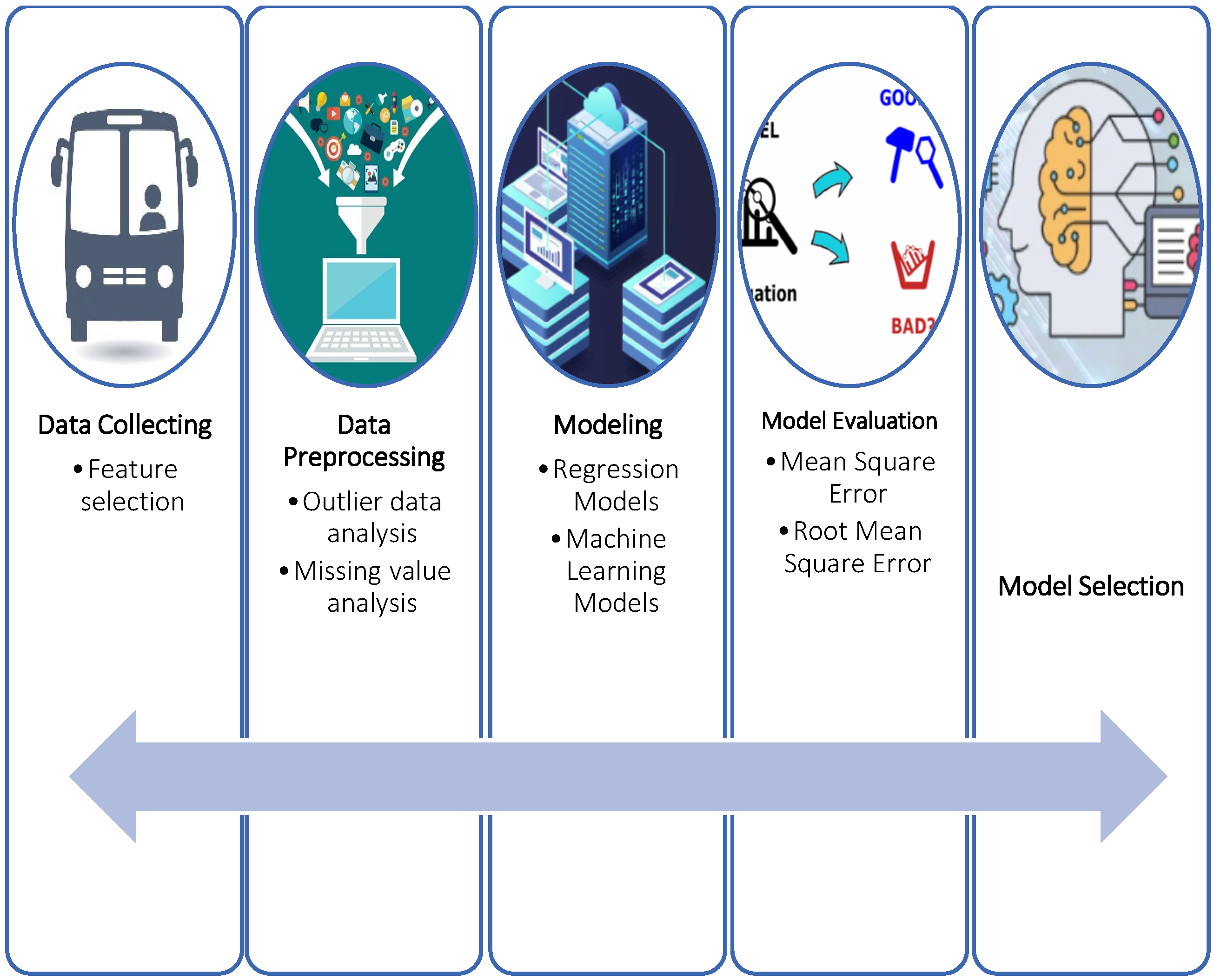
Figure 1. The framework of the study.
Applsci 16 00006 g001
Figure 2. Route map of R049 (The symbols indicate the bus stop locations along the selected route).
Applsci 16 00006 g002
Figure 3. Data Sample of the City Bus Line.
Applsci 16 00006 g003
Figure 4. The average travel time.
Applsci 16 00006 g004
Figure 5. Examples of observations that exceeded the standard travel time.
Applsci 16 00006 g005
Figure 6. The data preprocessing phases.
Applsci 16 00006 g006
Figure 7. The bar chart for missing values.
Applsci 16 00006 g007
Figure 8. The old data in datasets.
Applsci 16 00006 g008
Figure 9. The new data in datasets.
Applsci 16 00006 g009
Figure 10. The heatmap for the correlation between the independent and dependent variables.
Applsci 16 00006 g010
Figure 11. Outlier detection results using the LOF method.
Applsci 16 00006 g011
Figure 12. Threshold value used for outlier classification (13th ranked density).
Applsci 16 00006 g012
Figure 13. Data points identified as outliers (indices shown as IDs).
Applsci 16 00006 g013
Figure 14. The information in the dataset.
Applsci 16 00006 g014
Figure 15. The regression models and machine learning models used in this study.
Applsci 16 00006 g015
Figure 16. Graphical representation of MSE values for each algorithm (k = 4).
Applsci 16 00006 g016
Figure 17. Graphical representation of MSE values for each algorithm (k = 5).
Applsci 16 00006 g017
Figure 18. Heatmap of model performance (MSE) across different k values.
Applsci 16 00006 g018
Table 1. Travel time prediction studies.
AuthorsMethodsMain Conclusion/Weakness
Serin vd. [1]AdaBoost Regression, Gradient Boosted Regression, Random Forest Regression, Extra-Tree Regression, KNN Regression, Support Vector MachineEnsemble learning achieved higher accuracy than single algorithms, but no environmental or meteorological variables were included.
Gal vd. [2]Queueing Theory, Machine LearningProposed a hybrid queueing-ML model improving predictive reliability; however, weather effects and external disturbances were not considered.
Peterson vd. [3]Long Short-Term Memory (LSTM) Neural NetworkCaptured temporal and spatial dependencies effectively; interpretability was limited, and environmental variables were excluded.
Bai vd. [4]Support Vector Machines, Kalman FilteringCombined SVM and Kalman filter for dynamic prediction; effective for real-time data but sensitive to noise and parameter tuning.
Treethidtaphat vd. [5]Deep Neural Network, Ordinary Least Square (OLS) RegressionDNN outperformed OLS in travel time prediction, yet the model required large datasets and lacked contextual (e.g., weather) factors.
Chen vd. [6]Linear Regression, The Least Absolute Shrinkage and Selection Operator, K-Nearest Neighbors Regression, Support Vector Regression, Gradient Boosting Regression, The Long Short Term Memory Network, Bi-Directional Long Short-Term Memory, Seasonal Auto-Regressive Integrated Moving AverageComprehensive comparison of multiple ML and statistical models; improved accuracy but ignored environmental influence and interpretability.
Ashwini et al. [7]Linear Regression, Ridge Regression, Least Absolute Shrinkage and Selection Operator Regression, Support Vector Regression, K-Nearest Neighbors, Regression Trees, Random Forest Regression, Gradient Boosting RegressionShowed temporal and route-direction variables improve performance; however, no weather or external conditions were included.
Servos et al. [8]Extremely Randomized Trees, Adaptive Boosting (AdaBoost), Support Vector Regression (SVR)Ensemble algorithms outperformed mean-based approaches; dataset limited to freight transport and lacked meteorological diversity.
Ceylan and Özcan [9] Optimized bus frequencies using a meta-heuristic algorithm; not a predictive model and did not assess real-time variability.
Reddy et al. [10]Support Vector Regression (SVR)SVR improved prediction under variable traffic conditions; applicability restricted by small-scale data and absence of weather inputs.
Moosavi et al. [11]Chi-Square Automatic Interaction Detection, Random Forest, Gradient Boost TreeTree-based methods performed well across routes with differing frequencies; however, interpretability remained limited.
Wu et al. [12]ConvLSTM, LSTMIntegrated convolutional and recurrent structures enhanced temporal precision; required high computational cost and excluded weather factors.
Lee et al. [13]ConvLSTMUtilized spatio-temporal features for improved prediction; model complexity hindered practical deployment, and no environmental inputs were used.
He et al. [14]Interval-Based Historical Average Model, The Long Short Term Memory NetworkSeparated riding and waiting times for greater granularity; still limited by small-scale experiments and no weather analysis.
Table 2. Machine learning and regression algorithm studies.
AuthorsMethodsSubjectMain Conclusion/Weakness
Arslan and Ertuğrul [15]Multiple Regression Models, Artificial Neural Networks ModelsElectricity ConsumptionCompared to regression and ANN; ANN achieved better fit but model lacked robustness for non-linear volatility.
Fumo and Biswas [16]Simple Linear Regression Model, Multiple Linear Regression ModelEnergy ConsumptionRegression captured linear dependence on temperature; ignored nonlinearity and multivariable interaction.
Jang et al. [17]Linear Multiple Regression, Nonlinear Multiple Regression, Artificial Neural Networks (ANNs)Geological ParametersANN performed better than regression for complex relationships; interpretability was weak.
Nguyen and Cripps [18]Multiple Regression Models, Artificial Neural Networks ModelsHouse SalesANN outperformed regression; however, limited transparency and potential overfitting noted.
Talaat and Gamel [19]Correlation Coefficient, Multiple Linear RegressionNo. of Authors and No. of CitationsFound strong correlation between authorship and citation; regression model lacked causal interpretation.
Sun et al. [20]Random Forest AlgorithmResearch Octane NumberRF effectively modeled nonlinear fuel properties; dataset domain-specific, limiting generalizability.
Adami et al. [21]Principal Component Analysis (PCA), Principal Component Regression (PCR)Rheumatoid ArthritisPCA/PCR identified key clinical factors; medical focus unrelated to transport forecasting.
Yan et al. [22]Principal Component Regression, Partial Least Squares RegressionFlight Load AnalysisDemonstrated efficiency in handling multicollinearity; limited transferability to dynamic datasets.
Effendi et al. [23] Principal Component RegressionFarmer Exchange RateShowed PCR’s strength in dimensionality reduction; agricultural data context only.
Sing et al. [24]Principal Component Regression, Partial Least Squares RegressionPiperine Contents in Black PepperCompared regression methods for spectroscopy; not focused on time-dependent prediction.
Tahir and Ilyas [25]Robust Correlation-Based Regression, Robust Correlation Scaled Principal Regression Proposed robust approach for high-dimensional data; computationally heavy and untested in forecasting.
Lettink et al. [26]Ridge RegressionHealth IndicatorRidge regression reduced overfitting; performance limited by small sample.
Zandi et al. [27]Locally Weighted Linear Regression MethodThree Large-Scale Precipitation ProductsAchieved high spatial accuracy; model sensitive to regularization parameter.
Zhang et al. [28]Polynomial Ridge Regression (RR) AlgorithmAtomic NucleiEfficient for physics-based prediction; domain-specific with limited cross-field relevance.
Zheng et al. [29]Kernel Ridge Regression, Support Vector Machine (SVM), Artificial Neural Networks (ANNs)Wind SpeedKernel methods showed lowest error; required careful kernel tuning and large data.
Song et al. [30]Lasso Regression, Long Short-Term Memory Model (LSTM)Gas ConcentrationLasso improved variable selection; LSTM achieved higher accuracy but at higher complexity.
Li et al. [31]Lasso Regression, ARIMA, NARNN, LSTMCarbon PriceCombined classical and deep models; limited by temporal instability of financial data.
Sharma et al. [32]Linear Regression, Lasso Regression, Ridge RegressionStrength of GGBFSRegression performed well; lacks external validation and generalizability.
Didari et al. [33]Lasso RegressionWheat YieldIdentified key meteorological variables; effective locally but not tested on larger datasets.
Malakouti [34]Lasso Regression, Elastic Net AlgorithmsCarbon DioxideElastic net provided stable results; small dataset constrained robustness assessment.
Table 3. The variables and definitions.
VariablesDefinitions
DAYShows the days of the week.
1: Monday, 2: Tuesday, 3: Wednesday, 4: Thursday, 5: Friday, 6: Saturday, 7: Sunday.
AVERAGE_TEMPERATUREShows the average temperature during the day.
HUMIDITYShows the humidity rate during the day.
PRECIPITATIONShows the amount of precipitation per square meter during the day.
AIR_PRESSUREShows the air pressure.
AVERAGE_WIND_SPEEDShows the average wind speed during the day.
SCHEDULED_STARTING_TIMEShows the bus departure time scheduled by the transportation company.
NUMBER_OF_PASSENGERSShows the number of passengers who boarded the bus on the specified expedition.
Table 4. Numerical mean squared error (MSE) values of each algorithm for k = 4. Red font indicates the lowest MSE value in each column (best model performance). Shaded background highlights the best-performing algorithm for each parameter setting.
K ValuesThreshold ValueMultiple Linear
Regression
Principal Component RegressionRidge RegressionLasso RegressionElastic Net RegressionK-Nearest NeighborsMultilayer PerceptronClassification and
Regression Tree
Bagging Trees
Regression
Random Forest
Regression
Gradient Boost
Machine
Xgboost RegressionLight GBMCatboost
41025.1026.4726.4426.4226.4626.2624.0624.1123.1222.9523.1923.9023.8422.39
42021.5723.1222.7122.7322.7320.4120.5121.0719.6819.1219.1319.5119.4318.86
43021.6622.1022.4422.5022.4420.5618.8620.3118.5017.8618.1118.2618.3717.73
45019.1320.0419.7719.7919.8318.9618.5719.4518.6517.8317.8918.0518.0717.62
410018.7821.0719.1419.1519.1718.2318.0318.6817.8817.1917.2617.3917.4617.20
Table 5. Numerical mean squared error (MSE) values of each algorithm for k = 5. Red font indicates the lowest MSE value in each column (best model performance). Shaded background highlights the best-performing algorithm for each parameter setting.
K ValuesThreshold ValueMultiple Linear
Regression
Principal Component RegressionRidge RegressionLasso RegressionElastic Net RegressionK-Nearest NeighborsMultilayer PerceptronClassification and
Regression Tree
Bagging Trees
Regression
Random Forest
Regression
Gradient Boost
Machine
Xgboost RegressionLight GBMCatboost
51022.7025.7925.1525.1725.1425.2724.2023.2523.2423.0322.8823.9623.3522.52
52020.2425.1421.6021.6221.6320.4720.6620.9320.0819.2719.4419.6019.6519.09
53020.0121.6220.5220.5020.5419.7018.6419.2718.6717.8417.9617.8317.9917.95
55020.8121.7721.3321.2921.3619.2118.4419.3318.6417.8618.0518.0918.0517.59
510020.1722.2619.9419.9319.9818.3318.1818.3717.8217.0217.1017.0717.2016.80
Table 6. The mean squared error values of each algorithm (changing k values). Shaded background highlights the best-performing algorithm for each parameter setting.
K ValuesThreshold ValueMultiple Linear
Regression
Principal Component RegressionRidge RegressionLasso RegressionElastic Net RegressionK-Nearest NeighborsMultilayer PerceptronClassification and
Regression Tree
Bagging Trees
Regression
Random Forest
Regression
Gradient Boost
Machine
Xgboost RegressionLight GBMCatboost
410018.775821.066819.138119.153919.166518.230018.027418.675017.880517.193517.257617.392917.458017.1993
510020.171622.262119.935419.931819.982118.332418.183018.374717.819517.024717.103417.067217.197716.7975
610019.956726.887620.323820.341320.311118.153118.017518.601618.319917.208117.327917.193117.349816.9579
710018.945419.135619.120819.14719.161318.159217.772718.651218.010417.120317.172117.399517.252916.9975
810018.937520.971419.189819.201119.237618.091717.899818.389718.102717.049617.155817.062117.406616.7994
910020.886221.389821.355321.408421.399018.302218.023718.273117.803816.995117.175317.140917.282716.7951
1010020.875521.390521.357121.409521.399318.510318.187118.706517.370817.029217.078017.186817.177116.722
1510018.947019.653919.275119.263319.296018.272817.595818.635117.496917.061116.991717.283717.180716.9158
2010020.766421.214221.208921.262221.259518.574218.251618.611717.260216.940317.418717.17917.292816.7505
3010018.948524.653919.394519.405219.394318.164117.993917.948017.626717.110617.019717.044116.939116.7295
4010019.543221.053919.861119.899819.932618.302818.17618.000517.183617.133416.988517.148617.102416.6134
5010019.257319.511419.283419.255019.290418.102717.717618.132317.502516.858017.198417.172316.967916.5454
10010018.719318.782418.856718.867618.894318.097818.031817.771817.675816.900516.985717.142517.105416.7129
Table 7. Results of the Friedman test for model performance comparison.
HypothesisDescription
Null hypothesisH0: All treatment effects are zero
Alternative hypothesisH1: Not all treatment effects are zero
DFChi-Squarep-Value
12148.540.000
Disclaimer/Publisher’s Note: The statements, opinions and data contained in all publications are solely those of the individual author(s) and contributor(s) and not of MDPI and/or the editor(s). MDPI and/or the editor(s) disclaim responsibility for any injury to people or property resulting from any ideas, methods, instructions or products referred to in the content.