A Dual-Decomposition Graph-Mamba-Transformer Framework for Ultra-Short-Term Wind Power Forecasting

Abstract

Accurate ultra-short-term wind power forecasting is vital for the secure and economic operation of power systems with high renewable penetration. Conventional models, however, struggle with multi-scale frequency feature extraction, dynamic cross-variable dependencies, and simultaneously capturing local fluctuations and global trends. This study proposes a novel hybrid framework termed VMD–ALIF–GraphBlock–MLLA–Transformer. A dual-decomposition strategy combining variational mode decomposition and adaptive local iterative filtering first extracts dominant periodic components while suppressing high-frequency noise. An adaptive GraphBlock with MixHop convolution then models structured and time-varying inter-variable dependencies. Finally, a multi-scale linear attention-enhanced Mamba-like module and Transformer encoder jointly capture short- and long-range temporal dynamics. Experiments on a real wind farm dataset with 10-min resolution demonstrate substantial superiority over State-of-the-Art baselines across 1-, 4-, and 8-step forecasting horizons. SHAP analysis further confirms excellent consistency with underlying physical mechanisms. The proposed framework provides a robust, accurate, and highly interpretable solution for intelligent wind power forecasting.

1. Introduction

Driven by the global transition toward low-carbon energy and the large-scale integration of renewable resources, wind power has gradually become one of the main power sources in future energy systems [1]. In recent years, the installed capacity of wind power worldwide has continued to increase, and its share in the power generation mix has risen significantly, providing strong support for carbon emission reduction and energy security. However, wind power output was affected by multiple factors such as wind speed, turbulence intensity, meteorological disturbances, and terrain effects, exhibiting pronounced nonlinearity, non-stationarity, and randomness [2]. These characteristics often resulted in frequency fluctuations, increased reserve capacity, and higher wind curtailment rates, thereby threatening the security and economic efficiency of power system operations. Consequently, accurate wind power forecasting was of great importance for power dispatch optimization, renewable energy integration, and system operational security [3].

The development of wind power forecasting techniques has evolved from linear statistical models to machine learning and then to deep learning models [4]. Early statistical approaches—such as the ARIMA model, exponential smoothing, and multiple linear regression—were based on assumptions of stationarity and linearity [5]. They provided reasonable forecasts under short-term and stable conditions but struggled to capture the nonlinear mapping between wind speed and power output, remaining highly sensitive to noise disturbances [6]. With the advancement of computational capabilities, machine learning models such as SVM, RF, and GBDT [7,8] introduced nonlinear feature fitting and high-dimensional feature fusion, leading to notable improvements in prediction accuracy. Nevertheless, these models generally relied on manual feature engineering and failed to automatically extract multi-scale dynamic patterns from wind power sequences. Moreover, they provided a limited characterization of the time-varying coupling relationships among meteorological variables [9].

In recent years, the widespread application of deep learning in time-series modeling has further enhanced the accuracy of wind power forecasting. RNN, LSTM, and GRU models captured temporal dependencies through hidden state transmission, showing strong capability in nonlinear feature extraction [10,11]. Subsequently, CNNs were introduced to enhance local feature learning, while Transformer architectures demonstrated powerful performance in modeling long-term dependencies via self-attention mechanisms [12]. Despite these advances, conventional deep learning models still exhibited three major limitations in wind power forecasting:

Insufficient frequency-domain feature extraction: Wind power signals typically contain multi-scale periodic components and high-frequency noise. Direct time-domain modeling could not explicitly separate primary periodic patterns from disturbance components, leading to incomplete learning of periodic behaviors [13]. Limited cross-variable dependency modeling: In multi-meteorological-input scenarios, traditional models usually concatenated multiple variables as a single input sequence, failing to effectively capture the dynamic correlations and physical couplings among factors such as wind speed, temperature, and air pressure [14]. Inadequate balance between local fluctuations and global trends: Wind power sequences often exhibited both short-term volatility and long-term variations. Although deep networks possessed strong expressive capacity, they faced trade-offs between fine-grained detail capture and global trend representation [15].

To address these challenges, recent studies have proposed combining meteorological information with deep learning networks [16] or combining signal decomposition with hybrid deep modeling to improve the robustness and multi-scale representation of models. Methods such as EMD, EEMD, and VMD have been applied for denoising and feature extraction [17]. Hybrid models integrating deep learning, such as VMD-LSTM [18], CEEMDAN-GRU [19], and WT-CNN-LSTM [20], significantly enhanced prediction accuracy across different temporal scales. In addition to decomposition–sequence hybrid approaches, deep composite architectures combining CNN with recurrent or attention mechanisms—such as CNN-LSTM and LSTM-Transformer—have become popular for wind power forecasting by leveraging the strengths of different networks [21]. However, traditional decomposition–deep learning frameworks were often cascaded structures with weak coupling between the decomposition and forecasting modules, limiting the integration of signal decomposition, noise suppression, and dynamic modeling. Meanwhile, multivariate forecasting models mostly relied on temporal attention mechanisms and lacked explicit representation of graph-based dependencies among input variables.

To address the above challenges, this study develops a unified wind power forecasting framework (VMD–ALIF–GraphBlock–MLLA–Transformer) that integrates frequency–time analysis with cross-variable feature learning, aiming to enhance multi-scale representation, dynamic dependency modeling, and overall forecasting robustness.

In this study, the forecasting architecture is organized from a hierarchical multi-scale perspective, spanning micro-scale and meso-scale modeling layers, to address the intrinsic complexity of wind power time series. At the micro-scale, the framework focuses on fine-grained temporal fluctuations and high-frequency variations in wind power signals, which are critical for ultra-short-term forecasting accuracy. Without explicit decomposition and local temporal modeling, these rapid variations are easily obscured by noise or averaged out by global models. This level is primarily addressed through the VMD–ALIF dual decomposition, which separates local oscillatory components and suppresses noise, as well as through the Attention_Block that captures short-term temporal dependencies and abrupt dynamics. At the meso-scale, the model emphasizes structured inter-variable interactions and medium- to long-range temporal evolution, which cannot be effectively represented by simple variable concatenation or shallow temporal models. The GraphBlock explicitly models cross-variable dependencies among meteorological factors, while the MLLA and Transformer modules capture medium- and long-term temporal patterns with efficient global sequence modeling.

By explicitly organizing the model into micro-scale and meso-scale components, the proposed framework forms a problem-driven and hierarchical multi-scale learning paradigm, in which each module addresses a distinct and non-overlapping modeling challenge. This design integrates time–frequency decomposition, dynamic dependency modeling, and hierarchical temporal representation, rather than constituting a simple or redundant combination of independent algorithms.

2. VMD–ALIF–GraphBlock–MLLA–Transformer Forecasting Architecture

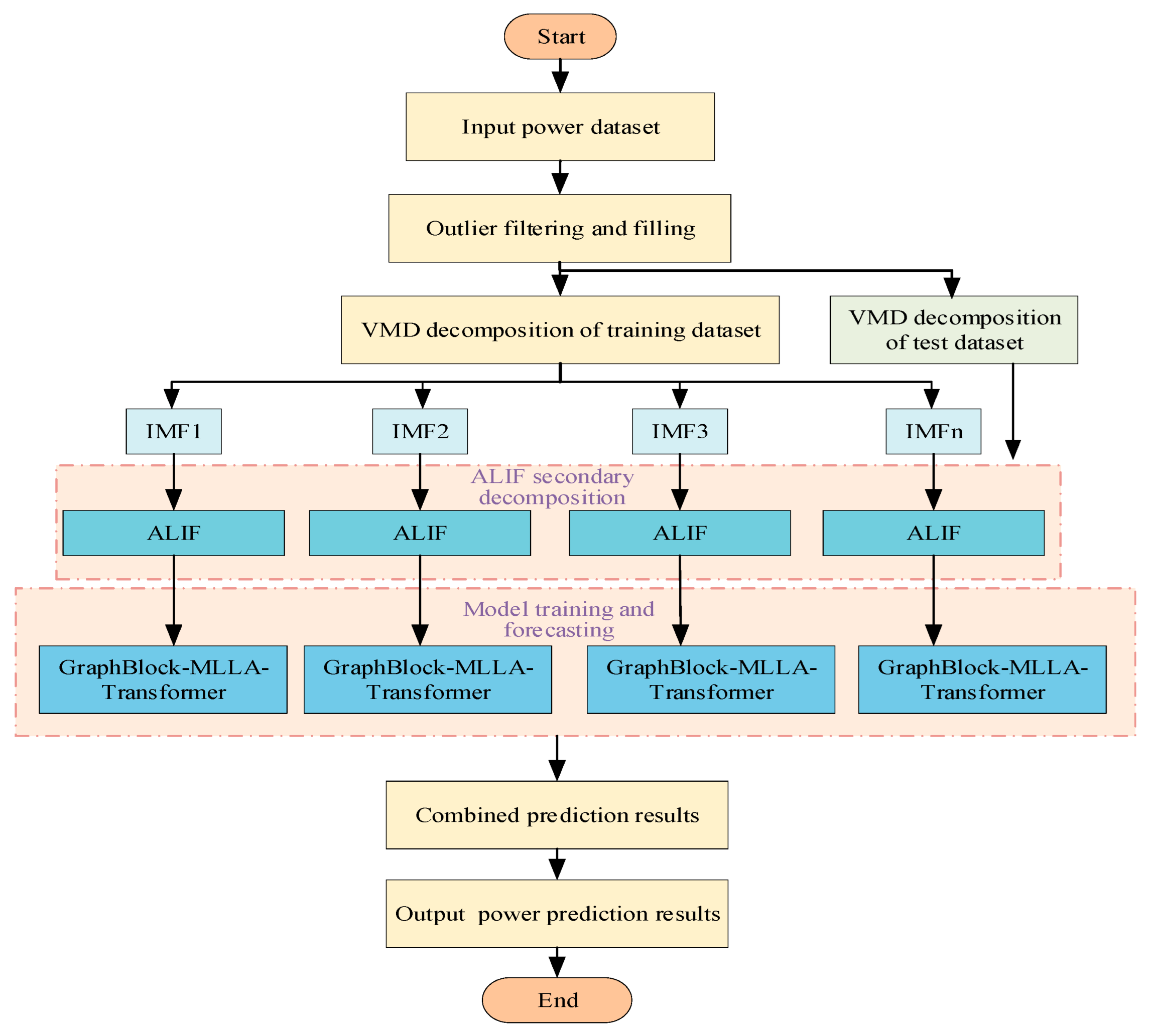
To enhance robustness and interpretability, the proposed forecasting architecture is designed as a hierarchical multi-scale framework, in which different modules operate at distinct temporal and structural scales, ranging from micro-scale local dynamics to meso-scale global evolution patterns. First, the original wind power signal is processed through Variational Mode Decomposition (VMD) to obtain modal components across distinct frequency bands. For modes with strong non-stationarity, Adaptive Local Iterative Filtering (ALIF) is further applied for secondary decomposition, yielding refined time–frequency representations and effectively suppressing high-frequency noise. This dual VMD–ALIF structure preserves signal integrity while enhancing feature discernibility and model robustness.

On this basis, a hierarchical deep architecture is constructed by combining a Graph Neural Network (GNN), a Selective State–Space Model (Mamba), a Multi-Scale Linear Attention (MLLA) module, and a Transformer encoder. The GNN captures structured dependencies among meteorological variables, Mamba preserves dynamic memory and filters critical state features, MLLA extracts multi-scale temporal details, and the Transformer models global temporal dependencies. Through the synergy of frequency-domain enhancement and cross-variable feature interaction, the proposed architecture achieves accurate and robust forecasting of wind power sequences. The overall framework of the model is illustrated in Figure 1.

It should be clarified that the proposed GraphBlock and MLLA modules do not aim to introduce new learning theories, but are task-oriented architectural designs that adapt existing methods to the specific challenges of wind power forecasting. GraphBlock is built upon adaptive graph learning and MixHop graph convolution, and its contribution lies in reformulating these techniques for multivariate meteorological time series to enable dynamic, data-driven modeling of inter-variable dependencies without predefined graphs. Similarly, MLLA is not proposed as a new attention mechanism, but rather as an efficient integration of linear attention and selective state–space modeling, inspired by recent Mamba architectures and well-suited for long-sequence and multi-scale temporal modeling.

Overall, the contribution of these components lies in problem-adaptive architectural integration, and their effectiveness is validated through systematic ablation and comparative experiments.

2.1. Dual Decomposition via VMD–ALIF

Wind power output is affected by multiple meteorological factors, resulting in multi-scale variability and local abrupt fluctuations in its time-series data. Traditional forecasting models relying on a single decomposition method often fail to capture both global trends and short-term variations simultaneously. To address this issue, a dual-layer decomposition strategy combining VMD and ALIF was proposed. In the first layer, VMD globally decomposes the raw power signal into a set of intrinsic mode functions (IMFs) with distinct frequency characteristics [22], where low-frequency modes represent long-term periodic patterns and high-frequency modes capture fast fluctuations and noise. To further refine components with strong local non-stationarity, ALIF is applied in the second layer [23]. By adaptively adjusting the filtering window and iteratively removing local means, ALIF extracts fine-scale variations related to transient environmental disturbances. This hierarchical VMD–ALIF framework effectively enhances time–frequency representation, mitigates mode mixing, and provides high-quality multi-scale features for downstream modeling.

Formally, the original power signal $f(t)$ was first decomposed by VMD into K modal components ${\{u_k(t)\}}_{k=1}^K$, allowing separation of global and periodic information across distinct frequency bands.

For a specific mode $u_k(t)$ containing substantial non-stationary information, ALIF was then applied for secondary decomposition to further separate its local oscillatory and smooth trend components. Let $x^{(0)}(t)=u_k(t)$ denote the initial signal. During the $i$-th iteration, the local mean was computed as

$$m^{(i)}(t)={\int }_{-\infty }^{+\infty }{x}^{(i)}(\tau )h^{(i)}(t-\tau )d\tau$$

(1)

where the window function $h^{(i)}(t)$ was adaptively updated according to the distribution of local extrema to capture the time-varying behavior of the signal:

$$\begin{array}{l}{h}^{(i)}(t)={\displaystyle \frac{1}{\sqrt{2\pi }{\sigma }^{(i)}(t)}}\exp \left(-{\displaystyle \frac{t^2}{2{[{\sigma }^{(i)}(t)]}^2}}\right)\\ {\sigma }^{(i)}(t)=\kappa \cdot L^{(i)}(t)\end{array}$$

(2)

with $L^{(i)}(t)$ representing the estimated distance between adjacent local extrema and $\kappa$ being a scaling constant.

The signal was iteratively updated following

$$x^{(i+1)}(t)=x^{(i)}(t)-m^{(i)}(t)$$

(3)

until the convergence criterion was satisfied.

$$x^{(i+1)}(t)-x^{(i)}(t)<ϵ$$

(4)

At convergence, $x^{(i)}(t)$ was defined as the local intrinsic oscillatory component $v_{k,j}(t)$, and the remaining part was treated as the smooth trend ${\tilde{u}}_k(t)$.

The low-frequency smooth component ${\tilde{u}}_k(t)$ captured the long-term trend of the signal, assisting the model in learning stable evolution patterns and predicting overall system dynamics. Meanwhile, the high-frequency detail component $v_{k,j}(t)$ reflected short-term fluctuations and instantaneous changes, enabling the model to respond rapidly to environmental variations or transient disturbances, thereby improving short-term forecasting accuracy.

After the two-stage decomposition, the wind power signal could be expressed as

$$f(t)={\displaystyle \sum _{k=1}^K\left[{\tilde{u}}_k(t)+{\displaystyle \sum _{j=1}^{J_k}{v}_{k,j}}(t)\right]}+r(t)$$

(5)

where $r(t)$ denotes the residual component.

The joint application of VMD and ALIF enabled fine-grained extraction of both global trends and local abrupt variations, effectively enhancing the model’s capability to represent complex nonlinear dynamics. Consequently, the proposed dual decomposition strategy improved both the accuracy and robustness of wind power forecasting by providing high-quality, multi-level feature representations for subsequent time-series modeling.

2.2. Forecasting Model

To simultaneously capture the intrinsic structure among multiple variables, short-term local variations, and long-term trends, this study proposes a novel multi-scale temporal forecasting framework. The architecture sequentially integrates a GraphBlock, MLLA, and Transformer module, enabling comprehensive modeling of inter-variable relationships and temporal dependencies in multivariate time series data. This design aims to enhance forecasting accuracy, particularly in complex, dynamic energy systems.

The ordering of GraphBlock, MLLA, and Transformer is deliberately designed based on their functional roles in representation learning, rather than arbitrarily selected. Specifically, the proposed architecture follows a progressive refinement strategy from inter-variable dependency modeling to hierarchical temporal representation.

GraphBlock is placed first to explicitly model dynamic dependencies among meteorological variables, enabling the network to construct structured variable-level representations before temporal aggregation. MLLA is then employed to efficiently capture medium- to long-range temporal dependencies over extended input sequences with reduced computational complexity. Finally, the Transformer module is applied to further refine global temporal representations and capture fine-grained long-term interactions.

This ordering ensures that temporal modeling is conducted on dependency-aware representations, thereby improving both modeling efficiency and forecasting accuracy.

2.2.1. GraphBlock: Adaptive Graph Convolution Module

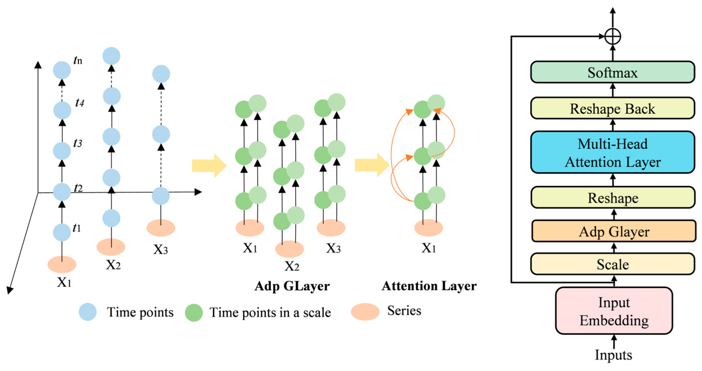
In multivariate time series forecasting, complex and dynamic dependencies often exist among variables—particularly in applications such as integrated energy systems and wind-solar power forecasting. Operational states at different locations, devices, or regions frequently influence one another. To effectively model such non-stationary structural correlations, we introduce an Adaptive Graph Learning mechanism that dynamically constructs a time-varying graph structure to represent inter-variable relationships [24].

Based on the learned graph, we apply MixHop Graph Convolution, which aggregates multi-hop neighbor information for feature extraction [25]. This enables deep, multi-scale, and cross-variable interaction modeling. By incorporating higher-order neighborhood features, the module not only enhances the model’s capacity to capture complex inter-variable dependencies but also supports the identification of both local and global dynamic behaviors in the system.

This design provides both theoretical and structural foundations for robust and accurate forecasting, offering strong adaptability to evolving system conditions. The architecture and operational principles of this module are illustrated in Figure 2.

(1)

Adaptive Graph Learning

In conventional GNNs [26], the adjacency matrix is typically predefined. However, in time series forecasting, dependencies among variables are often dynamic and time-varying. To address this, we employ an adaptive adjacency matrix learning mechanism that allows the model to automatically learn and update inter-variable dependencies during training.

Let $E_1\in {ℝ}^{N\times h}$ and $E_2\in {ℝ}^{N\times h}$ be trainable embedding parameters, where N denotes the number of variables and h denotes the embedding dimension. The adaptive adjacency matrix is defined as:

$$A=\mathrm{Softmax}\left(\mathrm{ReLU}\left(E_1{E}_2^T\right)\right)$$

(6)

where $E_1,E_2\in {ℝ}^{N\times h}$ are trainable node embeddings, h is the embedding dimension. The matrix product $E_1{E}_2^T$ computes pairwise similarity scores between variables. The ReLU activation removes negative values to ensure stability and interpretability. The Softmax function normalizes each row to ensure that the resulting weights form a valid probability distribution.

This formulation ensures that each row of A represents the learned correlation weights among variables, allowing the model to dynamically capture evolving interactions and optimize the graph structure during training.

(2)

MixHop Graph Convolution

1) Basic Graph Convolution

Once the adjacency matrix A is obtained, we perform Graph Convolution to propagate information among correlated variables [27]. The standard GCN operation is defined as:

$$H^{(1)}=\sigma (AX{W}^{(1)})$$

(7)

where $H^{(1)}$ is the output of the first graph convolution layer. $W^{(1)}$ is a trainable weight matrix. $\sigma (\cdot )$ is a nonlinear activation function. A is the information of each variable that can interact with its neighboring nodes.

While standard GCNs capture only first-order neighbor information, they struggle to model long-range dependencies across variables. To address this limitation, we adopt the MixHop mechanism for multi-order feature aggregation.

2) MixHop Mechanism

To simultaneously capture multiple levels of variable dependencies, we raise the adjacency matrix to different powers to represent higher-order interactions:

$$H^{(j)}=\sigma (A^{j}X{W}^{(j)}),\hspace{0.33em}\hspace{0.33em}\hspace{0.33em} j\in P$$

(8)

where P is the set of adjacency matrix powers, for example, P = {1,2} represents first-order and second-order adjacency propagation. $A^j$ represents the j-th power of the adjacency matrix, corresponding to j-hop neighborhood information.$W^{(j)}$ values are trainable weights for each propagation level.

Finally, we concatenated the information of all orders together:

$$H_{\mathrm{graph}}=\mathrm{Concat}(H^{(1)},H^{(2)},\dots ,H^{(P)})W_{\mathrm{mix}}$$

(9)

where $W_{\mathrm{mix}}$ is the trainable weight matrix after fusion.

By aggregating features across multiple propagation depths, MixHop enables the model to simultaneously capture both short-range and long-range dependencies. This enhances the representation of inter-variable structures and provides rich global information for downstream forecasting modules.

Unlike traditional GNNs that rely on manually defined graph structures, the GraphBlock learns inter-variable dependencies adaptively from the data. This makes it well-suited for time series forecasting tasks where the relationships among variables are implicit or dynamically evolving. In power prediction scenarios, this structure effectively models interactions among meteorological variables, thereby improving the overall forecasting performance.

2.2.2. Attention_Block: Multi-Head Self-Attention Module

The Attention_Block adopts a self-attention mechanism similar to that of the Transformer to capture local temporal dependencies and enhance the model’s ability to represent short-term dynamic variations. In multivariate time series forecasting tasks, the future state of a single variable is influenced not only by its own historical values but also by the short-term dynamics of other variables. Therefore, we employ a Multi-Head Self-Attention mechanism to learn these complex interaction patterns [28].

(1)

Query-Key-Value (QKV) Computation

Given an input sequence $X\in {ℝ}^{B\times L\times d}$, where B is the batch size, L is the sequence length, and d is the model dimension, the Q, K, and V matrices are obtained through linear projections:

$$Q=X{W}_q,\hspace{0.33em}\hspace{0.33em}\hspace{0.33em} K=X{W}_k,\hspace{0.33em}\hspace{0.33em}\hspace{0.33em} V=X{W}_v$$

(10)

(2)

Attention Weight Calculation

The attention weights measure the relevance between different time steps and are computed as follows:

$$A=\mathrm{Softmax}\left({\displaystyle \frac{Q{K}^T}{\sqrt{d_k}}}\right)$$

(11)

The scaling factor $\sqrt{d_k}$ prevents excessively large dot-product values, ensuring stable gradients. The softmax function normalizes the attention scores so that their sum equals 1, allowing the model to assign greater weight to more relevant temporal features.

(3)

Triangular Causal Mask

Since time series forecasting is an autoregressive task in which future information must not be used to predict the current time step, a causal mask M is introduced to enforce this constraint:

$$A=\mathrm{Softmax}\left({\displaystyle \frac{Q{K}^T}{\sqrt{d_k}}}+M\right)$$

(12)

$$M_{i,j}=\left\{\begin{array}{lll}0,\hfill & \mathrm{if} i\ge j\hfill & \hfill \\ -\infty ,\hfill & \mathrm{if} i<j\hfill & \hfill \end{array}\right.$$

(13)

This upper triangular masking matrix ensures that each time step can only attend to itself and previous time steps, preventing information leakage from the future.

(4)

Attention-Weighted Summation

The final attention output is obtained by applying the attention weights to the value matrix:

$$H_{\mathrm{attn}}=AV$$

(14)

This operation enables the current representation to incorporate information from relevant past time steps. To enhance model expressiveness, multiple attention heads are employed in parallel, each capturing different local patterns:

$${\mathrm{head}}_k=\mathrm{Softmax}\left({\displaystyle \frac{Q_k{K}_k^T}{\sqrt{d_k}}}+M\right)V_k,\hspace{0.33em}\hspace{0.33em}\hspace{0.33em} k=1,2,\dots ,K$$

(15)

Finally, concatenating the results of all heads obtains the final output through linear transformation:

$$H_{\text{attn-final}}=\mathrm{Concat}({\mathrm{head}}_1,{\mathrm{head}}_2,\dots ,{\mathrm{head}}_K)W_O$$

(16)

where $W_O$ is the output transformation matrix that maintains the same dimension as the input in the final output $(B\times L\times d)$.

The Attention_Block focuses on learning short-term local dependencies within the temporal sequence. By leveraging multiple attention heads, it can attend to different local regions simultaneously, effectively capturing dynamic variations in time series data. This capability is particularly critical for forecasting power outputs, where short-term fluctuations and abrupt changes play a key role.

2.2.3. MLLA: Mamba-like Linear Attention

In the standard Transformer architecture, the computational complexity of attention mechanisms scales quadratically with the sequence length $O(L^2)$. When applied to long-sequence modeling, this results in rapidly increasing computational overhead, making the model inefficient and resource-intensive for analyzing and forecasting power data with high-frequency sampling and extended time spans [29,30].

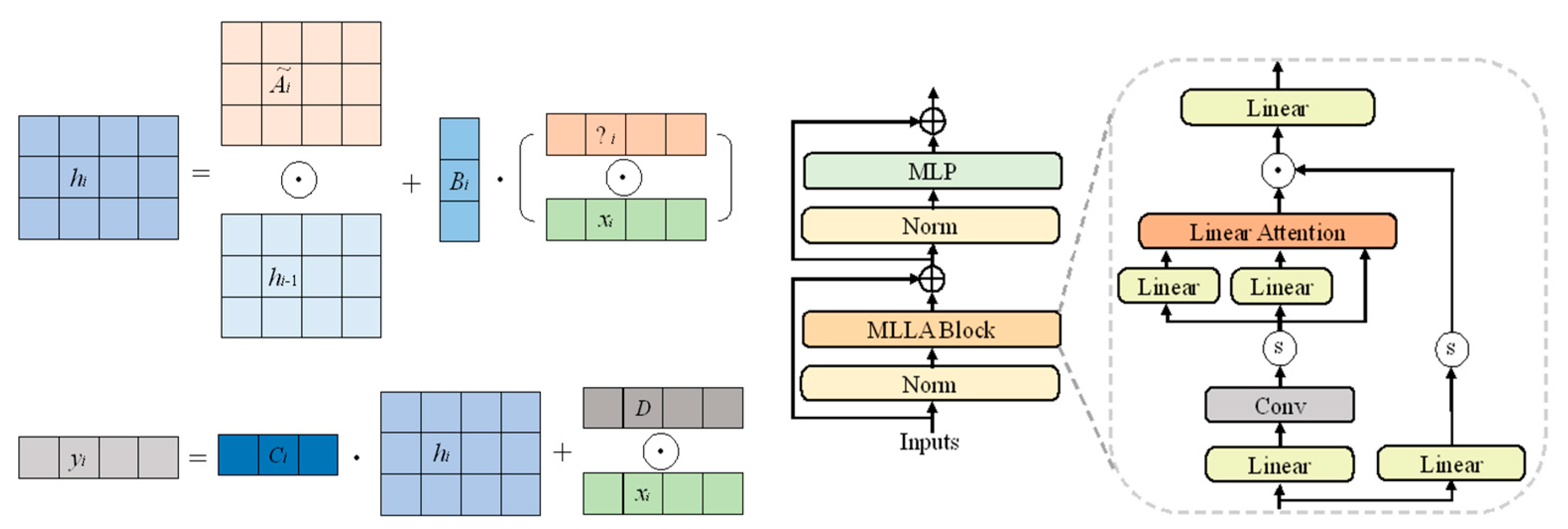
To address this challenge, an MLLA module is introduced [31]. MLLA integrates linear attention and the Mamba selective state–space model to enhance both efficiency and modeling capability [32].

Structurally, the MLLA adopts a linear attention mechanism, which reduces the computational complexity of the attention operation from $O(L^2)$ to $O(L)$, thereby significantly improving computational efficiency and scalability in processing long time series. This is particularly advantageous for real-time or large-scale forecasting scenarios.

Furthermore, the MLLA incorporates state–space modeling principles by using a continuous-time dynamical system to capture temporal dependencies within the sequence. This design enables the module to exhibit stronger long-term memory and better represent long-range dependencies. Such capabilities are crucial for capturing the underlying long-term structures in power output data, ultimately enhancing the predictive performance of ultra-short-term forecasting models.

The principle and architecture of the MLLA module are illustrated in Figure 3.

(1)

Derivation of Linear Attention Formulation

In the standard Transformer, attention scores are computed based on the dot product between the query (Q) and key (K) matrices:

$$A=\mathrm{Softmax}\left({\displaystyle \frac{Q{K}^T}{\sqrt{d}}}\right)$$

(17)

$$H_{\mathrm{attn}}=AV$$

(18)

where $Q,K,V\in {ℝ}^{L\times d}$ represent the query, key, and value matrices, L denotes the sequence length, and d is the model dimension.

Because the attention matrix A stores $L\times L$ pairwise scores, the computational complexity is $O(L^2)$, making it inefficient for long sequence tasks.

To alleviate this issue, the MLLA module adopts linear attention without Softmax normalization, which uses a kernel function $\varphi (\cdot )$ to map both queries and keys into a new feature space:

$$\begin{array}{l}{K}^{\varphi }=\varphi (K),\hspace{0.33em}\hspace{0.33em}\hspace{0.33em} Q^{\varphi }=\varphi (Q)\\ H_{\mathrm{mlla}}={\displaystyle \frac{Q^{\varphi }\cdot (K^{\varphi T}V)}{Q^{\varphi }\cdot K^{\varphi T}}}\end{array}$$

(19)

where $\varphi (\cdot )$ is a nonlinear feature mapping function [33], allowing the dot-product attention to be restructured into matrix multiplications.

Due to the associative property of matrix multiplication, $K^{\varphi T}V$ can be precomputed and reused across all time steps, calculating $Q^{\varphi }$ and its product again, reducing the computational complexity from $O(L^2)$ to $O(L)$. This formulation retains the ability to capture global contextual information while significantly lowering computational costs, making it suitable for long-sequence scenarios such as high-resolution power data forecasting.

(2)

Mamba Recursive State–Space Formulation

1) Standard State–Space Model (SSM)

The MLLA module also incorporates principles from the Mamba Selective State–Space Model, a class of temporal models grounded in the continuous dynamics of time series. A standard SSM is defined as:

$$\begin{array}{l}{h}_i=A{h}_{i-1}+B{x}_i\\ y_i=C{h}_i+D{x}_i\end{array}$$

(20)

where $h_i$ denotes the hidden state at time step i, representing historical information. $x_i$ is the current input, and $y_i$ is the output. A, B, C, D are learnable transition matrices.

2) Mamba Selective SSM

Inspired by Mamba, the MLLA modifies the standard SSM using gated mechanisms to control information flow adaptively:

$$\begin{array}{l}{h}_i={\tilde{A}}_i\odot h_{i-1}+B_i\left({\Delta }_i\odot x_i\right)\\ y_i=C_i{h}_i+D\odot x_i\end{array}$$

(21)

where ${\tilde{A}}_i$ is a forget gate, dynamically adjusting the contribution of historical information, enabling variable-length memory retention. ${\Delta }_i$ is an input gate, modulating the impact of the current input on the hidden state. $B_i, C_i, D$ are learnable parameters.

This recursive structure offers enhanced capacity for long-range dependency modeling, while mitigating the diffusion of information commonly encountered with Softmax-based attention. Compared to traditional Transformers, Mamba’s gated recurrence mechanism more effectively retains relevant information over long time spans and lowers computational cost, making it well-suited for ultra-long sequence modeling, such as wind power forecasting tasks.

The MLLA module thus serves as the core global sequence model, operating on features extracted from preceding layers. Its linear computational complexity provides a distinct advantage in handling long sequences efficiently, while the gate-controlled memory dynamics improve the model’s ability to maintain key information and enhance prediction accuracy.

2.2.4. Transformer: Global Feature Integration and Final Prediction Module

After passing through the GraphBlock, Attention_Block, and MLLA modules, the model obtains intermediate representations that capture multivariate structural dependencies, local dynamic variations, and long-term temporal patterns. These representations reflect topological relationships among variables, short-term fluctuations, and long-range trends, forming a multi-scale, cross-dimensional feature foundation.

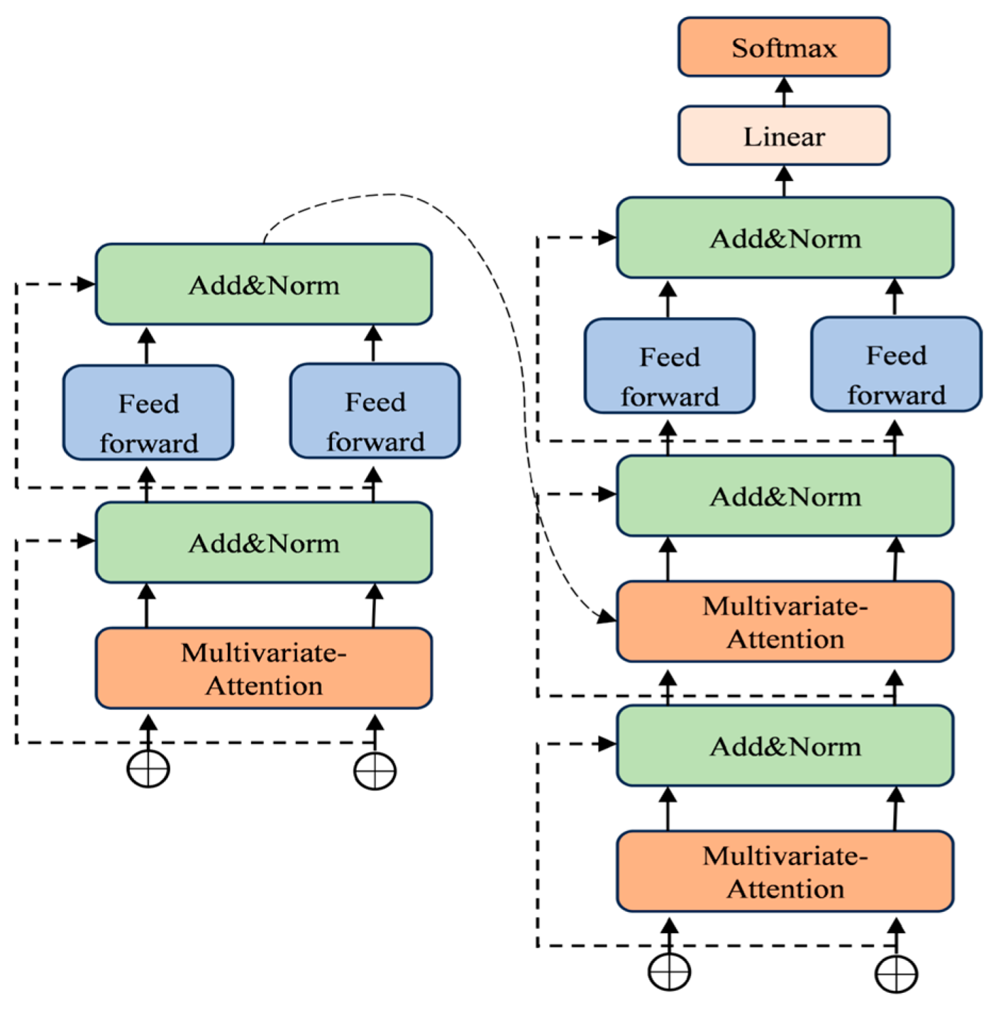
To further integrate these features and enhance overall modeling capability, this study incorporates a Transformer structure at the prediction stage for global feature fusion and final forecasting [34]. By leveraging multilayer stacked self-attention mechanisms, the Transformer can directly model dependencies across any positions in the sequence, offering strong global modeling capacity and high computational parallelism. The structure of the Transformer module is illustrated in Figure 4.

(1)

Standard Transformer Architecture

The Transformer module primarily consists of a multi-head self-attention mechanism and a feedforward neural network (FFN). The core computation of multi-head attention is given by:

$$H_{\mathrm{mba}}=\mathrm{Softmax}\left({\displaystyle \frac{(X{W}_i^Q){(X{W}_i^K)}^T}{\sqrt{d_k}}}\right)(X{W}_i^V)$$

(22)

The multi-head attention mechanism enhances the expressive capacity of the Transformer by enabling it to attend to different patterns across various time steps, thereby improving its ability to model temporal dependencies. After computing the multi-head attention output $H_{\mathrm{mba}}$, a FFN is applied to further transform the features:

$$H_{\mathrm{ffn}}=\sigma (W_1{H}_{\mathrm{mha}}+b_1)W_2+b_2$$

(23)

Here, $W_1, W_2$ are trainable weight matrices, and $b_1, b_2$ denote a nonlinear activation function used to enhance the model’s nonlinearity. This structure is essentially a two-layer multilayer perceptron designed to improve the representational capacity of the features.

The final output of each Transformer layer is expressed as:

$$H_{\text{trans-final}}=H_{\mathrm{ffn}}+H_{\mathrm{mha}}$$

(24)

Residual connections are applied to stabilize the training process, while layer normalization (LayerNorm) is employed to facilitate convergence:

$$H_{\mathrm{out}}=\mathrm{LayerNorm}(H_{\text{trans-final}})$$

(25)

(2)

Future Time Step Prediction

The output $H_{\mathrm{out}}$ from the Transformer is passed through a linear projection layer to map it to the target dimension:

$$\widehat{X}=W_{\mathrm{pred}}{H}_{\mathrm{out}}+b_{\mathrm{pred}}$$

(26)

where $W_{\mathrm{pred}},b_{\mathrm{pred}}$ are a trainable projection matrix. This layer transforms the high-dimensional representation produced by the Transformer into the final prediction values.

Within the proposed architecture, the Transformer serves as the final module responsible for global feature integration and prediction. After the preceding modules have separately captured the inter-variable structural relationships (GraphBlock), local short-term dependencies (Attention_Block), and efficient long-range dependencies (MLLA), the Transformer further fuses these multi-scale features to perform comprehensive global modeling and forecasting.

Its deep layered structure enables the model to capture more complex feature interactions without losing critical information over long sequences. Coupled with the FFN for enhanced feature transformation, the Transformer improves the model’s ability to express fine-grained temporal patterns, thereby enhancing prediction accuracy and robustness across diverse forecasting scenarios.

3. Case Study

3.1. Data Source

Given that the integrated energy system investigated in this paper incorporates a wind power generation module, we select wind power forecasting as a representative task to empirically validate the proposed hierarchical multi-module prediction model. This case study aims to evaluate the model’s effectiveness and practical applicability in handling complex temporal data.

The experimental data are obtained from operational monitoring records of wind turbines at a real-world wind farm. The dataset spans from 00:00 on 15 January 2024 to 23:50 on 31 December 2024, with a sampling interval of 10 min, resulting in a total of 50,688 complete data samples. Each sample consists of six key features: wind direction, wind speed, air density, turbulence intensity, wind shear below hub height, and actual power output of the wind turbine. All measurements are collected using high-precision sensors installed on on-site meteorological masts.

In the experimental setup, the input sequence length is set to 144, corresponding to 24 h of historical data used as input to the model. The prediction horizons are set to 1, 4, and 8 steps, corresponding to 10-min, 40-min, and 80-min ultra-short-term forecasting tasks, respectively. A rolling forecasting strategy is employed, where the model iteratively outputs the prediction for the next target time step, which is then used as part of the input for the subsequent prediction. This strategy simulates the continual update requirements typical in real-world operational forecasting scenarios.

3.2. Data Preprocessing

In addition to standard statistical preprocessing, domain-specific characteristics of wind energy conversion and practical constraints of wind farm measurement systems are explicitly considered to enhance data quality and physical consistency.

From a wind energy perspective, wind power output is inherently bound by turbine operational limits, including cut-in, rated, and cut-out wind speed regions. Consequently, abnormal power values that violate physical constraints—such as non-zero power under near-zero wind speeds or power exceeding rated capacity—are treated as potential measurement artifacts and removed. Moreover, due to the highly nonlinear relationship between wind speed and power, short-term turbulence may induce abrupt fluctuations that are not representative of the underlying energy conversion process. These effects motivate the adoption of robust statistical outlier detection rather than fixed threshold-based filtering.

From the measurement system perspective, the dataset is derived from SCADA records with a 10-min sampling interval, where each data point represents an averaged measurement. Such systems are susceptible to sensor noise, temporary communication interruptions, and synchronization delays among meteorological sensors and power meters. As a result, missing values and isolated abnormal samples occur intermittently, but they account for a relatively small proportion of the total dataset.

Based on these considerations, a statistical outlier detection method based on the mean and standard deviation is adopted:

$$\mu ={\displaystyle \frac{1}{N}}{{\displaystyle \sum }}_{i=1}^N{x}_i$$

(27)

$$\sigma =\sqrt{{\displaystyle \frac{1}{N}}{{\displaystyle \sum }}_{i=1}^N{(x_i-\mu )}^2}$$

(28)

Any data point satisfying $\mid x_i-\mu \mid >3\sigma$ is identified as an outlier. This criterion is selected to balance robustness and sensitivity, and empirical tests indicate that moderate variations around this threshold do not significantly affect forecasting performance.

Detected outliers and missing values are imputed using forward or backward filling, depending on data availability at neighboring time steps. Forward filling is applied when subsequent valid observations are unavailable, while backward filling is used otherwise. This strategy preserves temporal continuity while avoiding the introduction of artificial dynamics, which is particularly important for ultra-short-term forecasting.

By combining physically informed screening with statistically robust preprocessing, the resulting dataset maintains consistency with wind energy conversion mechanisms and SCADA measurement characteristics, thereby improving both reproducibility and reliability for subsequent model training and evaluation.

3.3. Effectiveness of VMD-ALIF Decomposition

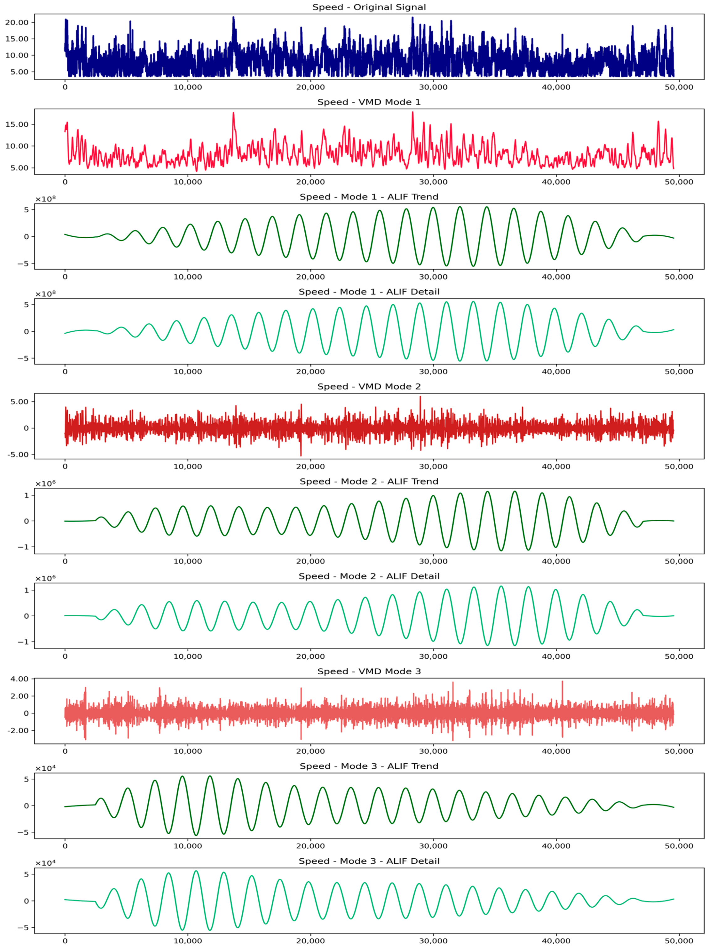
The original wind speed signal exhibits strong fluctuations and complex multi-scale variation patterns, including both long-term trends and short-term volatility. This reflects the typical non-stationary nature of wind speed time series, which poses challenges for direct modeling and prediction. To address this, a dual-stage decomposition strategy combining VMD and ALIF is applied prior to forecasting.

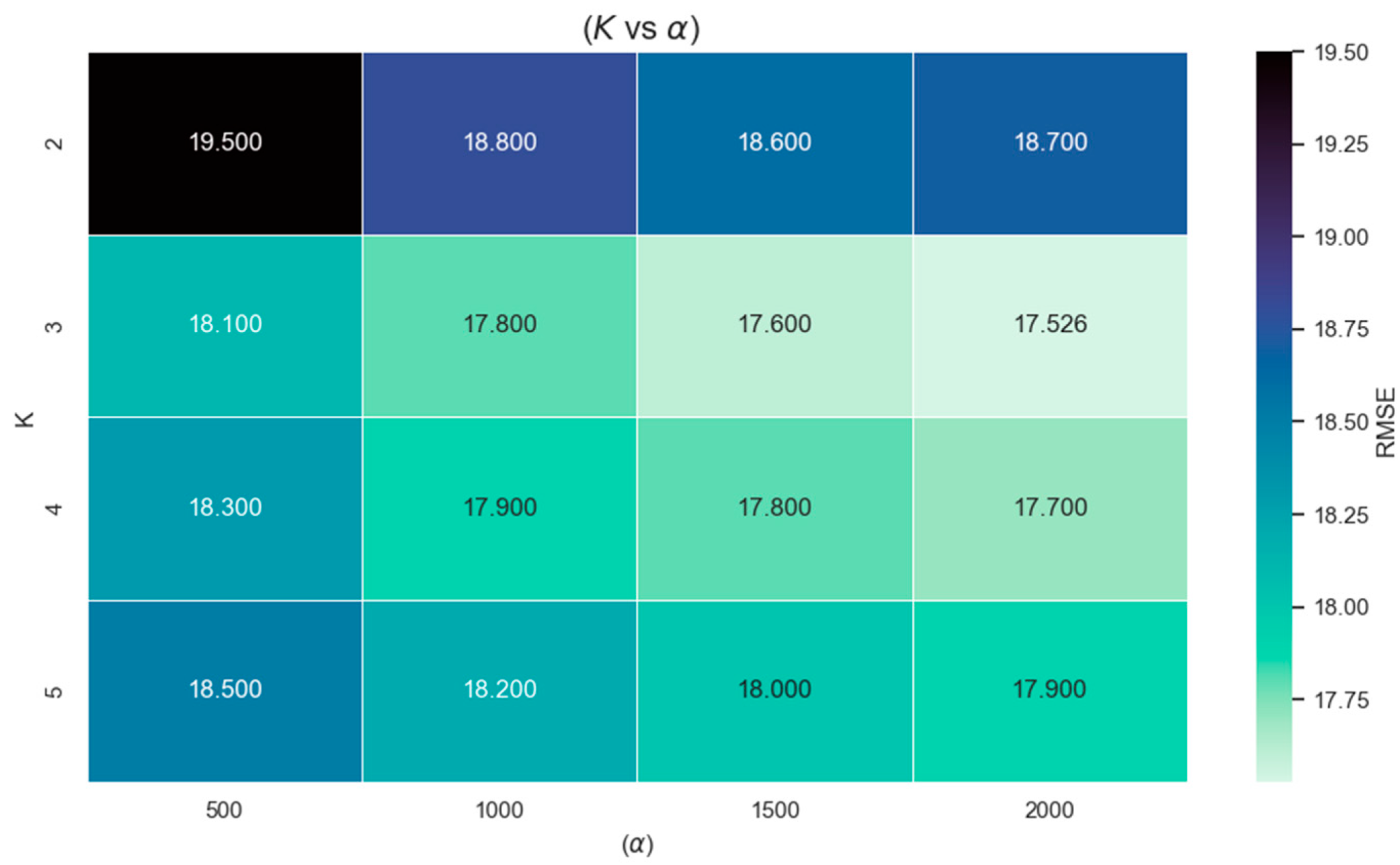
To optimize the key parameters of VMD, namely the mode number $K$ and the penalty factor $\alpha$, this study employs a grid search strategy combined with validation set evaluation to enhance the prediction accuracy of the downstream forecasting model. The search space is defined as $K\in \left[2, 8\right]$(integers) and $\alpha \in \left[500, 5000\right]$ with a step size of 500. Using the RMSE on the validation set as the optimization objective, all $\left(K,\alpha \right)$ combinations are evaluated in terms of their impact on forecasting performance.

The results, summarized in Figure 5, indicate that the configuration $K=3$ and $\alpha =2000$ yields the lowest validation RMSE (17.526). This configuration decomposes the wind power series into three physically interpretable sub-modes, corresponding to low-frequency trend components, mid-frequency periodic variations, and high-frequency stochastic disturbances. Compared with smaller values of $K$, this setting avoids under-decomposition that mixes heterogeneous frequency contents, while larger values of $K$ tend to introduce redundant or spurious modes, leading to marginal performance degradation. These observations suggest that the forecasting performance is moderately sensitive to the choice of $K$, but remains stable within a reasonable range.

For the ALIF stage, the window size is adaptively determined based on the local extrema distribution of each VMD mode, following the standard ALIF formulation. As a result, no fixed window length needs to be manually specified. This adaptive mechanism allows the filtering process to automatically adjust to local signal characteristics, reducing sensitivity to parameter tuning and enhancing robustness across different operating conditions. Empirically, the forecasting results remain stable under small variations in the ALIF scaling factor, indicating low sensitivity of the model performance to ALIF-related parameters.

Overall, the adopted VMD–ALIF parameter settings achieve a balance between decomposition fidelity and robustness, providing stable multi-scale representations for subsequent forecasting while avoiding excessive sensitivity to hyperparameter selection.

Figure 6 illustrates the layer-by-layer processing effect during the VMD-ALIF decomposition. Starting from the original signal, VMD first separates it into three distinct modes, each corresponding to a specific frequency band. Mode 1 represents low-frequency components with smooth variations, highlighting the long-term trend of wind speed. Mode 2 captures mid-frequency oscillations, effectively expressing medium-term disturbances. Mode 3 extracts high-frequency information, including sharp local fluctuations and noise. The bandwidth constraint imposed by VMD reduces frequency overlap across modes, thereby mitigating mode mixing and laying a reliable foundation for subsequent ALIF decomposition.

ALIF is then applied to each VMD mode to extract trend and detail components. For Mode 1, the trend displays low-frequency periodic oscillations that reflect the dominant cyclic behavior, while the detail captures localized variations with small amplitudes. In Mode 2, the trend retains periodicity with a slightly higher frequency than Mode 1, while the detail exhibits larger amplitude fluctuations that capture medium-scale variability. In Mode 3, the trend still maintains certain periodic characteristics but shows reduced stability, and the detail reveals intense short-term oscillations, reflecting strong local dynamics in the high-frequency domain.

The adaptive windowing of ALIF enables effective extraction of localized structural features, enhancing the interpretability of the decomposition. The combined VMD–ALIF process constructs a dual-scale hierarchical representation that separates the complex wind power signal into frequency-specific and trend–detail components. This structure highlights essential features, reduces non-stationarity, and facilitates more stable and accurate model training.

3.4. Results of the Hybrid Model

To comprehensively evaluate the performance of the proposed VMD–ALIF–GraphBlock–MLLA–Transformer model in wind power forecasting, multiple comparative experiments were conducted. The experimental evaluation includes representative baseline models, such as iTransformer [35] and Powerformer [36], which have demonstrated strong performance in general time series forecasting and wind power forecasting tasks. In addition, a series of progressively enhanced variants of the proposed model are constructed, in which key structural components are introduced in a step-by-step manner to systematically assess their individual contributions. Each model was evaluated under 1-step, 4-step, and 8-step forecasting tasks to examine both short-term and multi-step prediction capabilities.

Four widely used error metrics were adopted as evaluation criteria: the Root Mean Square Error (RMSE), Mean Absolute Error (MAE), Symmetric Mean Absolute Percentage Error (sMAPE), and the Coefficient of Determination (R²) [37]. These indicators jointly assessed the model’s accuracy, robustness, and generalization ability.

The benchmark and comparison models employed in this study are summarized in

Table 1. Comparison Model Abbreviation Table.

Model	Abbreviations
Transformer	#1
LSTM	#2
GraphBlock-Transformer	#3
MLLA-Transformer	#4
GraphBlock -MLLA-Transformer	#5
ALIF- GraphBlock -MLLA-Transformer	#6
VMD- GraphBlock -MLLA-Transformer	#7
VMD-ALIF- GraphBlock -MLLA-Transformer	#8
iTransformer	#9
Powerformer	#10

.

All models were trained and tested on the same dataset using identical input sequence lengths and rolling forecasting strategies. The prediction step sizes of 1, 4, and 8 were selected to assess each model’s ability to respond to short-term fluctuations and capture long-term trends across different temporal horizons.

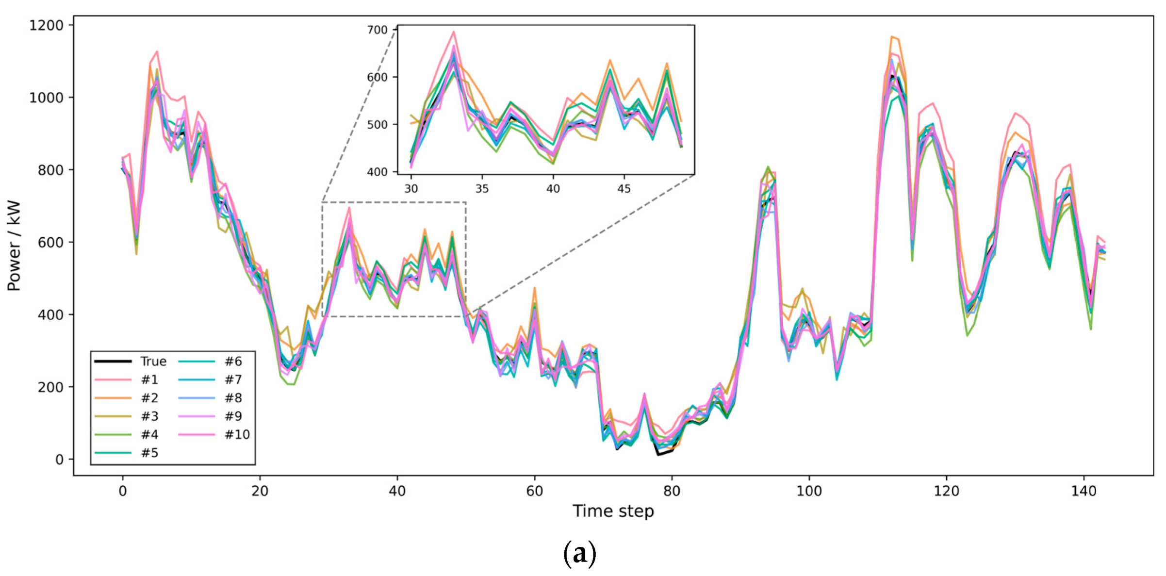
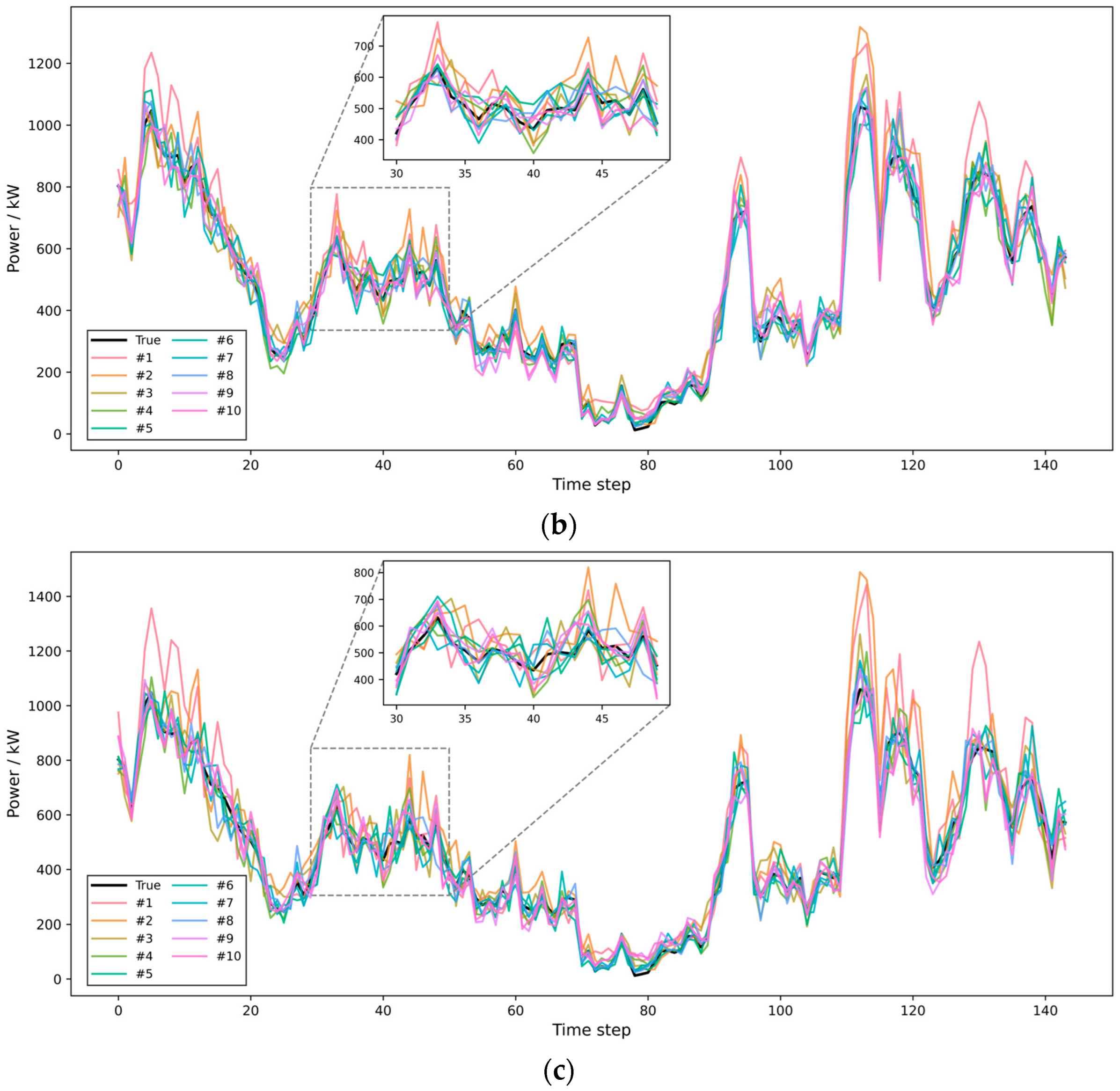
A unified set of evaluation metrics—including RMSE, MAE, sMAPE, and R²—was employed to ensure fair and consistent performance comparisons. These metrics offer a multi-perspective view of model accuracy, robustness, and generalization ability. The prediction results are presented in Figure 7 and

Table 2. Comparison of model evaluation results.

Model	Evaluation Metrics	Evaluation Result
		1-Step	4-Step	8-Step
#1	RMSE	49.628	86.455	120.168
	MAE	39.0994	61.900	81.753
	sMAPE	12.450	15.778	18.356
	R2	96.389	89.040	78.825
#2	RMSE	43.187	75.533	109.009
	MAE	34.637	58.370	74.147
	sMAPE	10.247	14.161	16.814
	R2	97.265	91.634	82.575
#3	RMSE	39.114	51.375	66.566
	MAE	29.250	42.089	51.523
	sMAPE	10.449	12.590	14.184
	R2	97.757	96.130	93.503
#4	RMSE	31.791	46.347	55.895
	MAE	25.282	35.187	43.538
	sMAPE	8.835	11.117	12.990
	R2	98.518	96.850	95.419
#5	RMSE	22.668	41.094	50.890
	MAE	17.799	32.047	38.876
	sMAPE	6.665	9.339	10.958
	R2	99.247	97.524	96.203
#6	RMSE	20.619	40.317	48.759
	MAE	16.287	29.486	37.271
	sMAPE	6.402	8.371	10.561
	R2	99.377	97.616	96.514
#7	RMSE	19.754	38.990	48.541
	MAE	15.980	29.516	37.246
	sMAPE	6.556	8.535	10.253
	R2	99.428	97.771	96.545
#8	RMSE	17.526	36.021	46.234
	MAE	13.838	26.598	33.903
	sMAPE	5.745	7.804	9.372
	R2	99.550	98.097	96.866
#9	RMSE	24.540	44.166	53.768
	MAE	18.985	36.375	42.105
	sMAPE	8.086	11.471	13.739
	R2	99.117	97.140	95.761
#10	RMSE	22.888	42.884	52.796
	MAE	18.597	33.985	41.083
	sMAPE	8.055	11.109	13.793
	R2	99.232	97.303	95.913

, where Figure 7a–c respectively depict the forecasting outcomes for the 1-step, 4-step, and 8-step settings.

As shown in the evaluation results from Figure 7 and Table 2, the proposed VMD-ALIF-GraphBlock-MLLA-Transformer model (Model #8) consistently outperforms all baseline and comparison models across different prediction horizons in terms of both accuracy and stability in the wind power forecasting task. Specifically, for the 1-step prediction task, the RMSE of the proposed model is reduced to 17.526, representing a 64.7% decrease compared to the baseline Transformer model (Model #1, RMSE = 49.628). Even compared with the GraphBlock-MLLA-Transformer without signal decomposition (Model #5, RMSE = 22.668), the proposed model still achieves a 22.7% reduction. The MAE is also reduced to 13.838, marking a 64.6% improvement over Model #1 (MAE = 39.099).

In the 4-step prediction scenario, the proposed model achieves an RMSE of 36.021 and an MAE of 26.598, which are 58.3% and 57.0% lower, respectively, than those of the baseline model (RMSE = 86.455, MAE = 61.900). Even when compared with structurally enhanced models such as Model #6 and Model #7, the proposed model demonstrates superior performance, highlighting the synergistic benefits of the dual decomposition strategy via VMD and ALIF. The performance improvements are primarily attributed to the model’s ability to integrate multivariate structural information and temporal dependencies with a two-stage decomposition framework.

In medium- to long-term forecasting scenarios, such as the 8-step prediction task, the proposed model continues to deliver strong performance, with an RMSE of 46.234 and an MAE of 33.903, significantly outperforming all other models (e.g., Model #1 yields an RMSE of 120.168). This demonstrates the robustness and generalization capacity of the proposed architecture in handling long-sequence dependencies and multi-scale feature modeling.

Moreover, in terms of the sMAPE and the R²—two comprehensive evaluation metrics—the proposed model also exhibits superior performance across all prediction horizons. The sMAPE values are 5.745%, 7.804%, and 9.372%, and the R² scores reach 99.550%, 98.097%, and 96.866% for the 1-step, 4-step, and 8-step predictions, respectively. These figures are significantly better than those of the baseline model, which achieves sMAPE scores of 12.450%, 15.778%, and 18.356%, and R² scores of 96.389%, 89.040%, and 78.825%. The notable reduction in sMAPE indicates improved control over relative error across various power levels, while the higher R² reflects a more accurate fit to actual power variation trends with smaller residuals, further validating the model’s advancement in handling the non-stationarity and multi-scale structure of wind power data.

In summary, by leveraging modular decomposition, structural integration, and information enhancement mechanisms, the proposed model achieves significant reductions in prediction error, improved robustness, and enhanced fitting accuracy across various forecast horizons. These results demonstrate the model’s high potential for practical application in complex time series prediction tasks such as wind power forecasting.

3.5. Wind Speed Variation Analysis

To further assess the robustness and generalization of the proposed model under sharp wind speed fluctuations, a dynamic indicator—the two-step wind speed change rate—is introduced. This metric quantifies the variation between the current wind speed and that two steps earlier (20 min interval), effectively reflecting the intensity of local turbulence.

Compared with conventional metrics such as RMSE and MAE that evaluate overall accuracy, this indicator focuses on model performance during rapid wind variations. Since wind power is strongly influenced by wind speed and exhibits high nonlinearity, maintaining low prediction errors under such conditions demonstrates the model’s adaptability to non-stationary environments and its practical robustness.

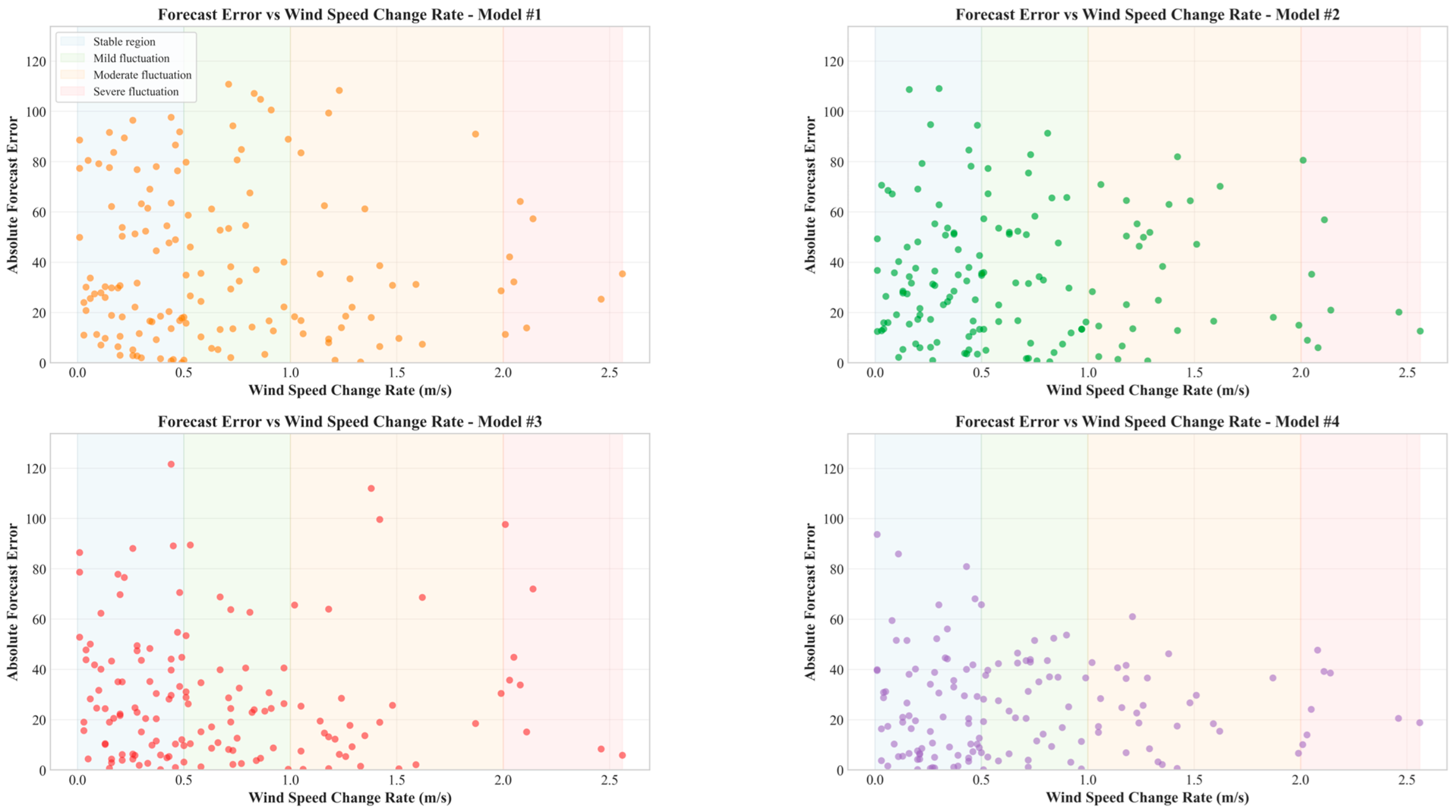
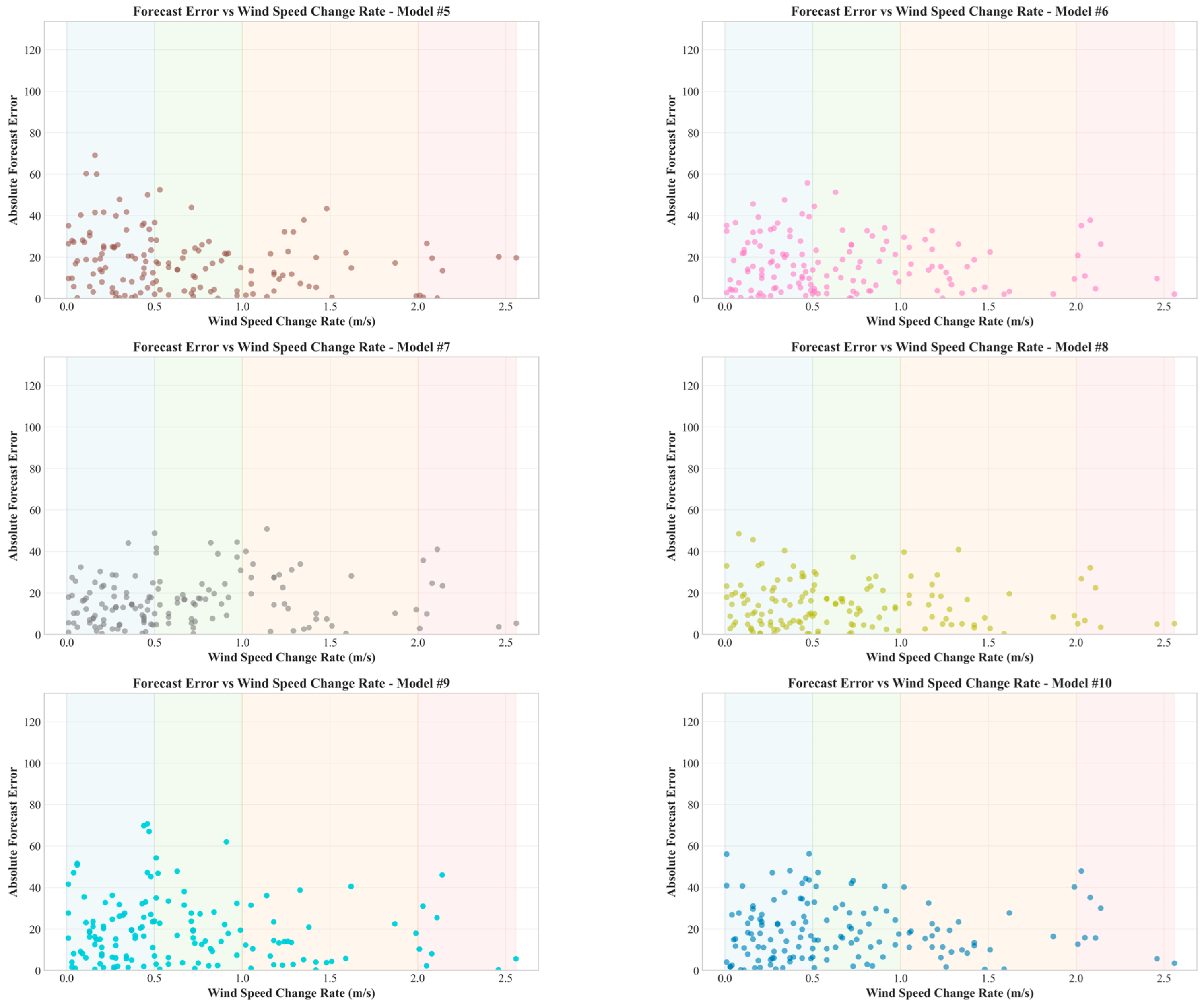
In this study, the absolute forecast errors of the model are analyzed in relation to the corresponding wind speed change rate, with the results visualized as shown in Figure 8.

According to the simulation results, the proposed VMD-ALIF-GraphBlock-MLLA-Transformer model consistently maintains low forecasting errors across different ranges of wind speed variation, demonstrating superior dynamic adaptability and robustness. Specifically, when the wind speed change rate approaches zero (indicating relatively stable wind conditions), all models exhibit low forecasting errors; however, the proposed model still outperforms others in accuracy.

In regions where the wind speed change rate exceeds 1.0—indicating intense turbulence—conventional models such as Transformer and LSTM show a marked increase in error, revealing their limited responsiveness to abrupt changes. In contrast, the proposed model maintains stable and low error levels even under such challenging conditions, with errors being more tightly distributed and no significant outliers observed. This highlights its strong prediction stability and resilience in dynamically fluctuating environments.

In conclusion, by incorporating a graph-based structure to effectively model inter-variable dependencies and combining the sequential modeling capabilities of MLLA and Transformer, the proposed model significantly enhances its robustness and generalization performance under scenarios involving rapid wind speed changes and extreme disturbances. These attributes make it well-suited for deployment in the highly dynamic environments typical of real-world wind power systems.

Wind power forecasting errors are strongly influenced by short-term wind speed fluctuations, which represent the primary exogenous disturbance in wind energy systems. While scatter plots provide intuitive insights into the relationship between wind speed variability and prediction errors, quantitative evaluation across different fluctuation regimes is necessary to rigorously assess model robustness. Therefore, this study further analyzes the error distribution of the proposed model under varying wind speed fluctuation intensities.

Specifically, wind speed fluctuation is characterized by the wind speed change rate, and all test samples are divided into four fluctuation regimes (Stable, Mild, Moderate, and Severe) using quartile-based thresholds. For each regime, the forecasting error is evaluated using MAE, RMSE, and error standard deviation to capture both accuracy and dispersion characteristics.

Table 3. Quantitative analysis results of the proposed model.

Band	MAE	RMSE	Standard Deviation
Mild	13.330	18.058	18.001
Moderate	14.389	17.195	16.797
Severe	11.376	14.538	14.521
Stable	16.371	19.944	19.944

quantitative results demonstrate that forecasting errors do not increase monotonically with wind speed fluctuation intensity. Instead, the largest errors are observed under stable wind conditions, while the lowest MAE and RMSE are achieved under severe wind speed fluctuations. This behavior can be attributed to the nonlinear wind speed–power relationship: under relatively stable and low wind speed conditions, small wind deviations may lead to amplified power prediction errors, whereas under higher fluctuation regimes the power curve becomes smoother and the proposed multi-scale model can more effectively capture dynamic patterns. Moreover, the close consistency between RMSE and error standard deviation across all regimes indicates stable error distributions without extreme outliers, confirming the robustness of the proposed framework against varying wind disturbance levels.

3.6. SHAP Analysis

To further examine whether the proposed model captures physically meaningful relationships rather than purely statistical correlations, SHAP (SHapley Additive exPlanations) analysis is employed to assess the contribution patterns of meteorological variables to wind power predictions [38]. It should be noted that SHAP does not explicitly encode physical equations into the model; instead, it provides a post hoc interpretability tool to evaluate whether the learned input–output relationships are consistent with established wind energy principles.

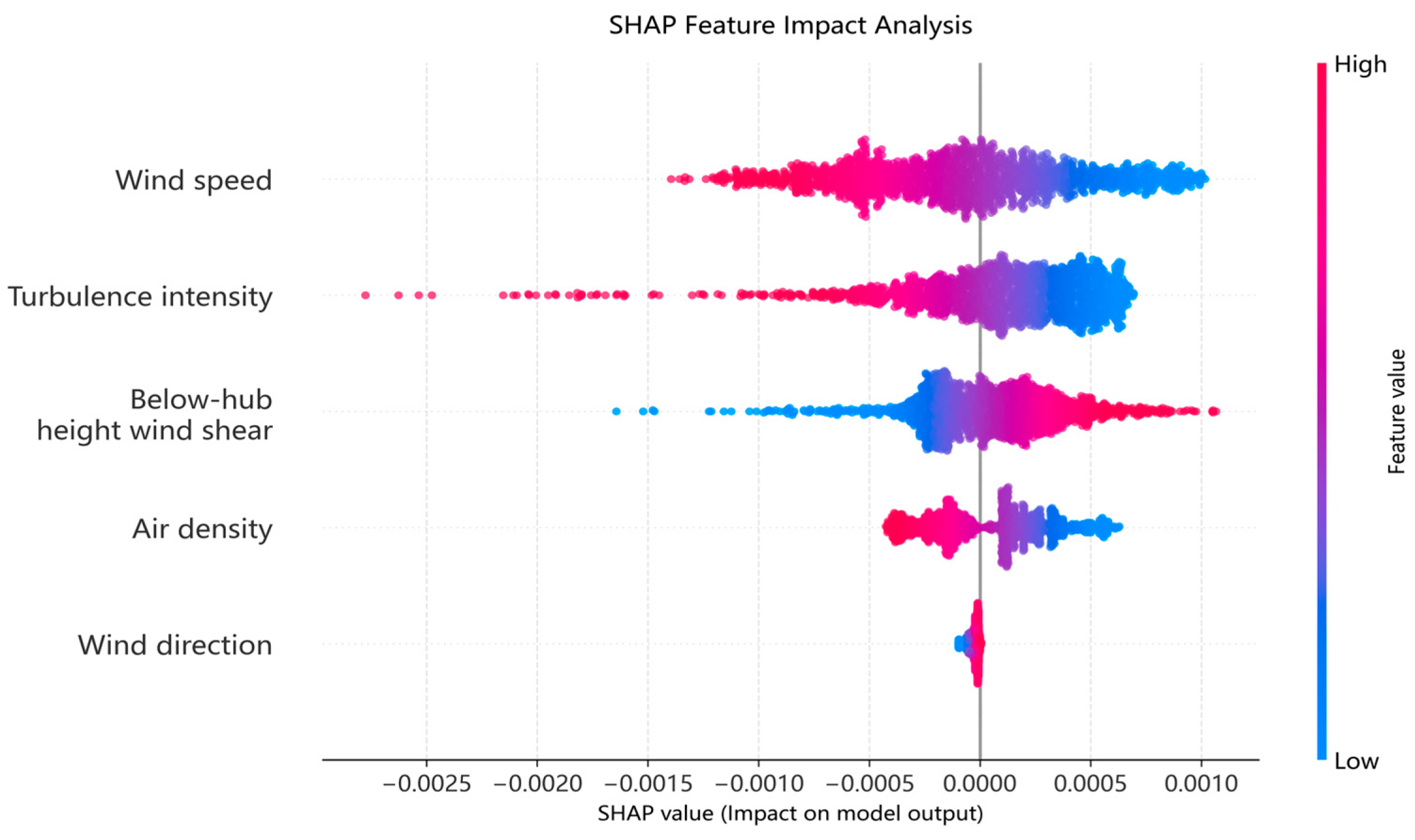
As shown in Figure 9, wind speed exhibits the largest SHAP magnitude and a consistently positive contribution to power output. This behavior aligns with the fundamental wind power conversion mechanism, in which higher wind speeds generally lead to increased power generation within the turbine’s operational range, reflecting the nonlinear nature of the wind speed–power relationship.

Turbulence intensity shows a predominantly negative SHAP contribution, indicating that increased turbulence reduces predicted power output. This observation is consistent with physical understanding, as high turbulence degrades aerodynamic efficiency and causes unstable inflow conditions, thereby limiting effective energy capture.

Air density and wind shear below hub height exhibit moderate but systematic contributions, suggesting that variations in atmospheric conditions influence power output through changes in aerodynamic loading and inflow profiles. In contrast, wind direction demonstrates a relatively minor impact, which can be attributed to the yaw control systems of modern wind turbines that actively align the rotor with incoming wind, thereby mitigating directional effects.

Overall, the SHAP results demonstrate that the proposed model learns feature–response relationships that are physically interpretable and consistent with established wind energy principles. This consistency provides indirect but meaningful evidence that the model does not rely on spurious correlations, thereby enhancing confidence in its robustness and generalization capability.

4. Conclusions

This study proposed a VMD–ALIF–GraphBlock–MLLA–Transformer hybrid framework to address key challenges in wind power forecasting, including insufficient frequency-domain feature extraction, limited cross-variable dependency modeling, and the difficulty of balancing local fluctuations with global trends. The VMD–ALIF module performed multi-scale time–frequency decomposition to extract dominant periodic components and suppress high-frequency noise. The GraphBlock captured structured dependencies among meteorological variables, modeling their dynamic coupling with power output. The combination of MLLA and Transformer further fused local and global temporal features, enabling an accurate representation of complex non-stationary dynamics.

Experimental results showed that the proposed model consistently outperformed conventional baselines across wind farm datasets, confirming its superior accuracy and robustness. SHAP interpretability analysis demonstrated that the model effectively captured nonlinear relationships while maintaining consistency with physical mechanisms.

Overall, the proposed framework not only achieved substantial improvements in forecasting precision but also established a physically interpretable and generalizable deep learning paradigm. Although the proposed framework achieves promising forecast performance, several limitations should be noted. The current study focuses on data from a single wind farm, and further validation on multi-site datasets is required to assess generalization. In addition, the hybrid architecture increases model complexity compared with simpler baselines. However, model training is performed offline, and online forecasting only involves forward inference, which is compatible with real-time operation under typical SCADA sampling intervals. Future work will also consider robustness against data latency and missing measurements in practical deployments.