Article

Landslide Susceptibility Mapping Using a Stacking Model Based on Multidimensional Feature Collaboration and Pseudo-Labeling Techniques

School of Geophysics and Geomatics, China University of Geosciences, Wuhan 430074, China
*
Author to whom correspondence should be addressed.
Appl. Sci. 2026, 16(1), 430; https://doi.org/10.3390/app16010430 (registering DOI)
Submission received: 10 December 2025 / Revised: 27 December 2025 / Accepted: 27 December 2025 / Published: 30 December 2025

Featured Application

Firstly, we propose MFP_Stacking, an innovative stacking framework that uniquely integrates Random Forest, TabNet, LeNet, and Vision Transformer to achieve superior accuracy in landslide susceptibility mapping. Secondly, the introduced multidimensional feature collaboration strategy and semi-supervised pseudo-labeling technique effectively overcome the limitations of feature representation and mitigate the challenge of limited labeled samples. This method provides a robust and practical tool for generating more reliable landslide risk maps, which is crucial for disaster prevention and land-use planning in vulnerable areas; additionally, it constructs a generalizable AI framework that can effectively address the common challenges of feature representation and sample scarcity in geospatial predictive modeling.

Abstract

Landslides are geological hazards that endanger socioeconomic development and ecological security, with landslide susceptibility mapping (LSM) playing a critical role in risk management and spatial planning. Recently, ensemble learning (EL) models have gained attention for effectively addressing the limitations of individual deep learning (DL) models in LSM. However, EL models always built on single-pixel, multi-factor inputs struggle to capture the spatial structure features of terrain units, limiting their ability to depict complex disaster patterns. Moreover, the scarcity of landslide samples and high annotation costs constrain model performance in LSM. To overcome these challenges, we propose a Stacking model based on multidimensional feature collaboration and pseudo-labeling techniques, referred to as MFP_Stacking. A stacking EL model is first employed in MFP_Stacking to integrate global statistical attribute features extracted from one-dimensional vectors with multi-scale spatial topological features derived from three-dimensional vectors. This strategy of multidimensional feature collaborative modeling enhances the model’s ability to learn complex environmental patterns associated with landslides. Subsequently, pseudo-labeling techniques are adopted to incorporate unlabeled data into auxiliary training, thereby addressing the problem of sample scarcity. MFP_Stacking was applied to LSM in the Zigui–Badong section of the Yangtze River Basin and in Ya’an City, Sichuan Province. Experimental results demonstrate that the proposed model performs well in overcoming limitations in feature representation, alleviating sample scarcity, and enhancing the quality of LSM outcomes. It achieved an average improvement of 2.4% for the Zigui–Badong section and 2% for Ya’an City across various evaluation metrics compared to other models.

1. Introduction

Landslides are relatively common and highly hazardous geological disasters that are widely distributed and occur with high frequency, capable of destroying residential areas, disrupting transportation networks, damaging farmland and hydraulic infrastructure, and potentially triggering secondary disasters such as floods and debris flows [1]. Recent case studies further highlight the sudden and destructive nature of landslides. For example, the catastrophic winter landslide in Liangshui Village, Zhenxiong County, Yunnan Province, caused severe casualties [2].
Landslide susceptibility mapping (LSM) is crucial for disaster prevention, as it identifies high-risk areas and offers a scientific foundation for the implementation of mitigation measures [3]. A series of LSM algorithms were proposed. In general, LSM methods are categorized into deterministic and non-deterministic prediction models [4]. Deterministic models rely on large amounts of geological data and are sensitive to data quality, making it difficult to achieve accurate large-scale predictions. Non-deterministic models can be classified into knowledge-driven and data-driven approaches [5,6]. Knowledge-driven approaches have achieved promising results in LSM but still exhibit a high degree of subjectivity [7,8,9]. In contrast, data-driven methods do not require extensive physical data collection, and the training process is objective, making them suitable for large-area LSM. Traditional machine learning (TML) models, as data-driven approaches, have demonstrated outstanding performance in LSM tasks [10], such as Linear Regression [11], Logistic Regression [12,13] and Support Vector Machine (SVM) [14,15]. However, they are sensitive to sample noise and struggle to clearly interpret the nonlinear coupling mechanisms among influencing factors [16].
Recently, deep learning (DL) models, as data-driven approaches, have also demonstrated promising learning performance in LSM [17]. DL models possess stronger nonlinear learning capabilities and adaptability than TML models. A wide range of DL architectures, such as Convolutional Neural Network (CNN) [18,19], fully connected autoencoders [20], Residual Networks (ResNet) [21], Recurrent Neural Network (RNN) [22], U-Net [23], Graph Convolutional Network (GCN) [24], Deep Belief Network (DBN) [25], and Vision Transformers (ViT) [26,27], have been successfully applied to LSM. Notably, single models often struggle to capture spatial heterogeneity and complex interactions among multiple factors in landslide occurrences, particularly when dealing with the nonlinear and multi-scale characteristics of complex geological environments.
Ensemble learning (EL) models can integrate the feature representation capabilities of multiple single classifiers, thereby enhancing the overall performance in LSM compared to single models [28]. Researchers have developed EL models such as Stacking, Boosting, and Bagging by utilizing various machine learning and DL models as individual single classifiers [29,30]. For example, Bagging and Boosting models that employ multiple decision trees as single classifiers [31,32,33]; Bagging models that utilize various SVM variants as single classifiers [34]; and Stacking models that incorporate DBN, CNN, and Deep Residual Networks (DRN) as single classifiers [35]; and Stacking models constructed by randomly combining ten machine learning algorithms for landslide susceptibility assessment in Gacha County [36], among others. Among these models, Stacking demonstrates more favorable learning capability, as it adaptively optimizes the combination of single classifiers through a meta-model and effectively suppresses overfitting via cross-validation. However, these EL models rely solely on one-dimensional vectors composed of multi-factor information from individual pixels for modeling. While such point-based approaches effectively capture the global statistical relationships among conditioning factors, they fall short in learning the spatial structural characteristics of local terrain units, thereby limiting the model’s ability to represent complex disaster patterns. Moreover, although some studies have adopted three-dimensional vector-based modeling approaches to extract multi-scale spatial structural features, such as the application of ViT in LSM [27,37,38], these methods are typically implemented within a single model, which not only suffers from limited generalization capability but also lacks the ability to capture global statistical features.
In addition to the limitations of feature representation, sample scarcity is another critical challenge limiting the performance of EL models. Specifically, the incompleteness of historical landslide records and the high cost of annotation have resulted in a limited number of original landslide samples. In Stacking model, the application of N-fold cross-validation further reduces the volume of training data, thereby exacerbating the impact of sample scarcity on model performance. To address this issue, a variety of strategies have been proposed, such as generating additional landslide samples using Deep Convolutional Generative Adversarial Networks [39], enhancing feature representations through unsupervised learning [40], and expanding the sample pool based on environmental similarity, among others [41]. However, these methods strongly rely on prior assumptions regarding data generation processes or feature extraction mechanisms. Pseudo-labeling, a semi-supervised learning technique, has attracted considerable attention in recent years, particularly in scenarios where labeled data is scarce or costly to obtain [42,43,44]. It employs a pre-trained model to predict landslide occurrences from unlabeled multi-source environmental data within the study area, selecting high-confidence potential landslide points as pseudo-labeled samples to facilitate deep feature mining and augment the training dataset. This technique autonomously selects reliable samples without manual intervention, and its iterative optimization strategy generates pseudo-labels that better approximate the actual landslide distribution, while enhancing feature representation through a semi-supervised learning mechanism.
Based on the foregoing analysis, we propose a Stacking model based on multidimensional feature collaboration and pseudo-labeling techniques (MFP_Stacking) for LSM. MFP_Stacking employs multidimensional vectors and a Stacking model to achieve collaborative modeling of multidimensional features, while leveraging pseudo-labeling techniques for feature mining and data augmentation. This model overcomes the limitations of feature representation, alleviates the impact of limited samples, and significantly improves both prediction accuracy and the quality of landslide susceptibility zonation maps. The main contributions of this study are as follows:
(1)
A Stacking model is employed to integrate Random Forest (RF), TabNet, LeNet, and ViT methods, fully leveraging their complementary strengths in shallow rule extraction and deep semantic modeling.
(2)
To address the effects of limited feature representation on model performance, we propose a multidimensional feature collaborative modeling strategy. This strategy employs a Stacking model to integrate global statistical attributes extracted from one-dimensional vectors with multi-scale spatial topological features derived from three-dimensional vectors. Through this cross-dimensional feature collaboration, the model achieves unified representation learning, thereby enhancing its ability to characterize relevant environmental factors.
(3)
To address the issue of sample scarcity, we introduce the pseudo-labeling technique from semi-supervised learning. A dual-validation mechanism, combining self-training and multi-network collaboration strategies, is employed to generate high-confidence pseudo-labels. This method effectively exploits the latent feature information of unlabeled samples for auxiliary training, thereby improving model stability and generalization capability.
(4)
We validated the effectiveness of the proposed model using two representative study areas, Zigui to Badong in the Yangtze River Basin and Ya’an City in Sichuan Province, where it consistently outperformed traditional EL models across all accuracy metrics.

2. Study Area and Data

2.1. Study Area

To evaluate the model’s generalization capability and robustness, we selected two study areas: the Zigui–Badong section of the Yangtze River Basin and Ya’an City in Sichuan Province. The distinct climatic and geological conditions between these regions provide an effective basis for assessing the model’s adaptability.

2.1.1. The Zigui–Badong Section of the Yangtze River Basin

The study area lies in the western part of Xiling Gorge, Hubei Province, between 30.02–30.93° N and 110.30–110.87° E, encompassing a 2–4 km wide belt along both banks of the river, with a total length of about 55 km, as shown in Figure 1. The study area features a subtropical monsoon climate and is traversed by the Yangtze River and over 200 tributaries, with abundant water resources [45]. The study area features a karst mountainous landform with a narrow basin-like terrain, high around the edges and low in the center. The area mainly comprises mudstone, siltstone, and marl, featuring weak lithology and low stability [46]. The area’s unique geological and climatic conditions lead to frequent rainstorm-induced landslides.

2.1.2. Ya’an City in Sichuan Province

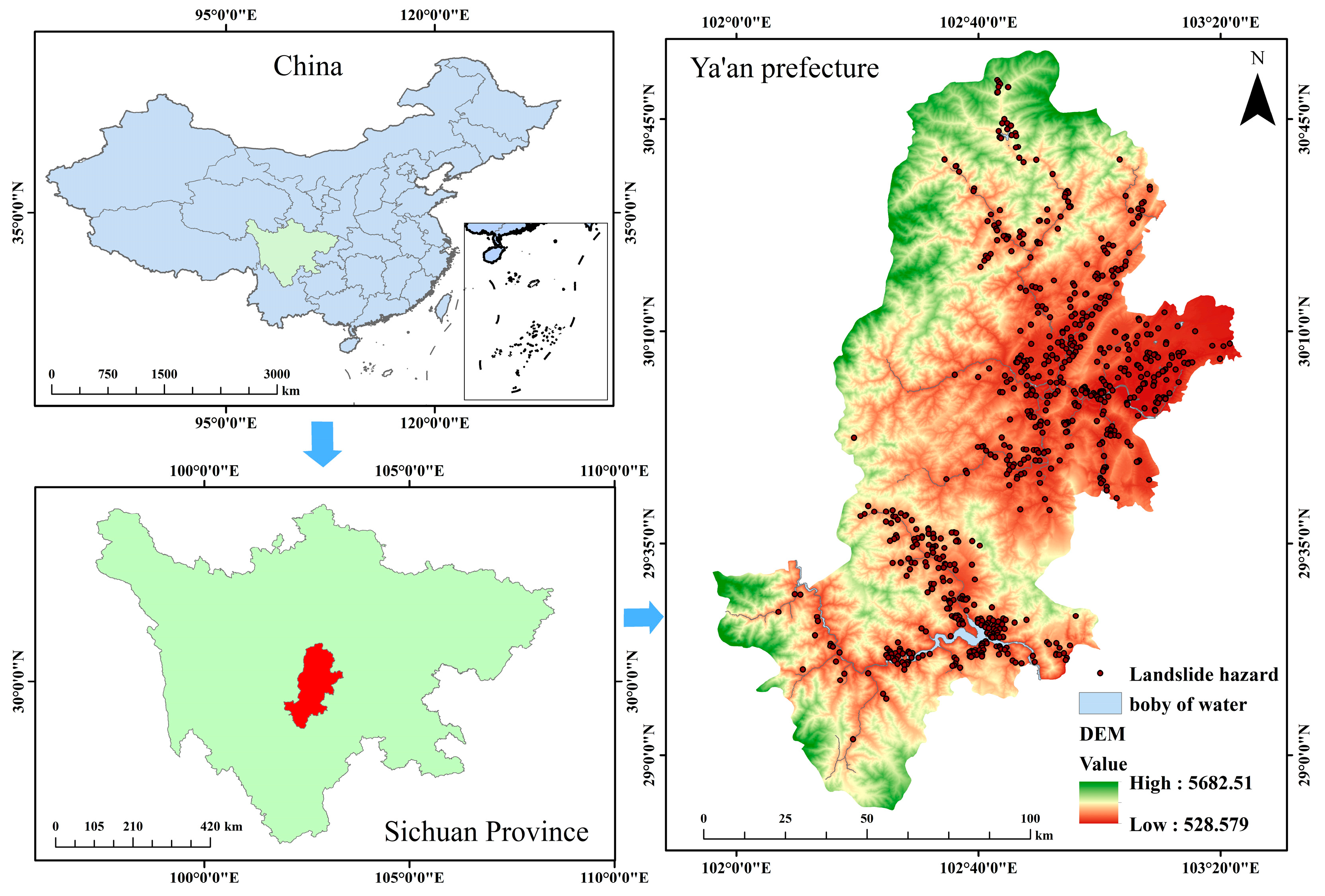
The study area is located in the western Sichuan Basin, spanning from 28.85–30.93° N and 101.92–103.38° E, as shown in Figure 2. The region lies within the subtropical humid monsoon climate zone, featuring a well-developed river system including the Dadu and Qingyi Rivers and their tributaries, with terrain gradually descending from northwest to southeast [47]. The region is geologically complex and tectonically active, with varied lithology: sandstone, shale, and limestone occur along basin edges and hills; schist and gneiss in mountainous zones; granite develops along fault belts with strong weathering [48].

2.2. Sample Preparation

2.2.1. Positive Sample

The landslide inventory map visually displays the spatial distribution of historical landslides, facilitating analysis of relationships between conditioning factors and landslide development while providing essential positive sample labels and a dataset construction basis for model training. In this study, we utilized point-based data of rainfall-induced landslides provided by the Resource and Environment Science Data Center of the Chinese Academy of Sciences to construct a landslide inventory map. The data included 197 points in the Zigui–Badong section and 737 in Ya’an City, as shown in Table 1.

2.2.2. Negative Sample

During model training, negative samples representing non-landslide areas are required to facilitate the learning of non-landslide characteristics. However, the original data does not contain such information. Therefore, a landslide susceptibility zonation map was generated for the study area using the information value method. Accordingly, an equal number of non-landslide points were randomly selected from the very low and low susceptibility zones on this map to serve as negative samples, as shown in Table 1.
The information value method [49] is a statistical approach that determines the weight of each category of a given factor by calculating the ratio between its landslide density (LD) and the overall LD, thereby enabling an objective assessment of landslide susceptibility. For a given factor, its information value is defined as:
I i = log 2 S i A i S A
where S i denotes the number of landslides within factor category i A i is the area of factor category i , S represents the total number of landslides, and A is the total area of the study region.
The total information value of each evaluation unit, which incorporates multiple influencing factors, is then calculated as:
I = I 1 + I 2 + I 3 + + I n
where n is the number of influencing factors. A higher value of I indicates a higher likelihood of landslide occurrence.
In this study, the information value model is used to generate non-landslide samples by selecting points located in areas with negative or relatively low information values. The information value has a clear physical interpretation, and areas with low values are quantitatively identified by the model as regions where geological and environmental conditions are unfavorable for landslide occurrence. Compared with simple random sampling, this approach effectively avoids potential high-susceptibility zones and reduces the risk of misclassification.

2.3. Landslide Conditioning Factors

Selecting Landslide conditioning factors (LCFs) is a crucial step in LSM. The ideal LCFs should meet three criteria: suitability for mathematical modeling, ease of quantification, and diverse distribution. In addition, factor selection should consider landslide types, regional characteristics, and data availability to ensure scientific validity and model reliability [50]. Based on these principles, we selected 11 indicators as LCFs for each study area: elevation, slope, aspect, plan curvature, profile curvature, lithology, distance to faults, land use, Normalized Difference Vegetation Index (NDVI), average annual rainfall, and distance to drainage.
Among the various LCFs, high-altitude steep terrain areas are susceptible to landslides because the high slope gradient increases the gravitational shear stress on the ground surface. This elevated gradient directly influences the stress distribution within the slope body, rendering steep slopes highly prone to instability under gravity [51]. Aspect determines solar radiation and weathering intensity, thereby influencing surface moisture evaporation and vegetation coverage, affecting slope stability. Curvature reflects terrain convexity and concavity, influencing surface runoff erosion, soil saturation, and stress distribution, thus impacting slope stability. Regarding lithology, weak rock layers with soft and loose structures are prone to water absorption and softening, leading to reduced shear strength and increased sliding risk. Near fault zones, rock masses are intensely fractured, increasing landslide risk. Land use patterns reflect the extent of human activity; excessive development can weaken the stability of slopes, while dense vegetation helps to consolidate the soil, thereby reducing the likelihood of landslides [52]. Regarding hydrology, groundwater increases pore water pressure and softens soil structure, while surface runoff induced by heavy rainfall can erode the slope, exacerbating the risk of landslides. The data sources for LCFs in each study area are shown in Table 2.
In addition, this paper uses grid cells for LSM studies, and all TIF format data need to have a uniform spatial resolution. Due to the diverse sources of the data, pixel sizes vary. Therefore, elevation data are employed as the reference in each study area, and other data are resampled to ensure that all data have the same resolution and spatial reference system.

2.4. LCFs Analysis and Selection

Before conducting landslide susceptibility modeling, it is necessary to perform correlation and importance analyses of the LCFs. Correlation analysis identifies the relationships between factors, removes highly correlated factors, reduces data noise, and prevents model overfitting. Importance analysis assesses the contribution of each factor to landslide occurrence, eliminating low-importance factors, which reduces computational complexity and enhances the model’s operational efficiency.

2.4.1. Multicollinearity Analysis

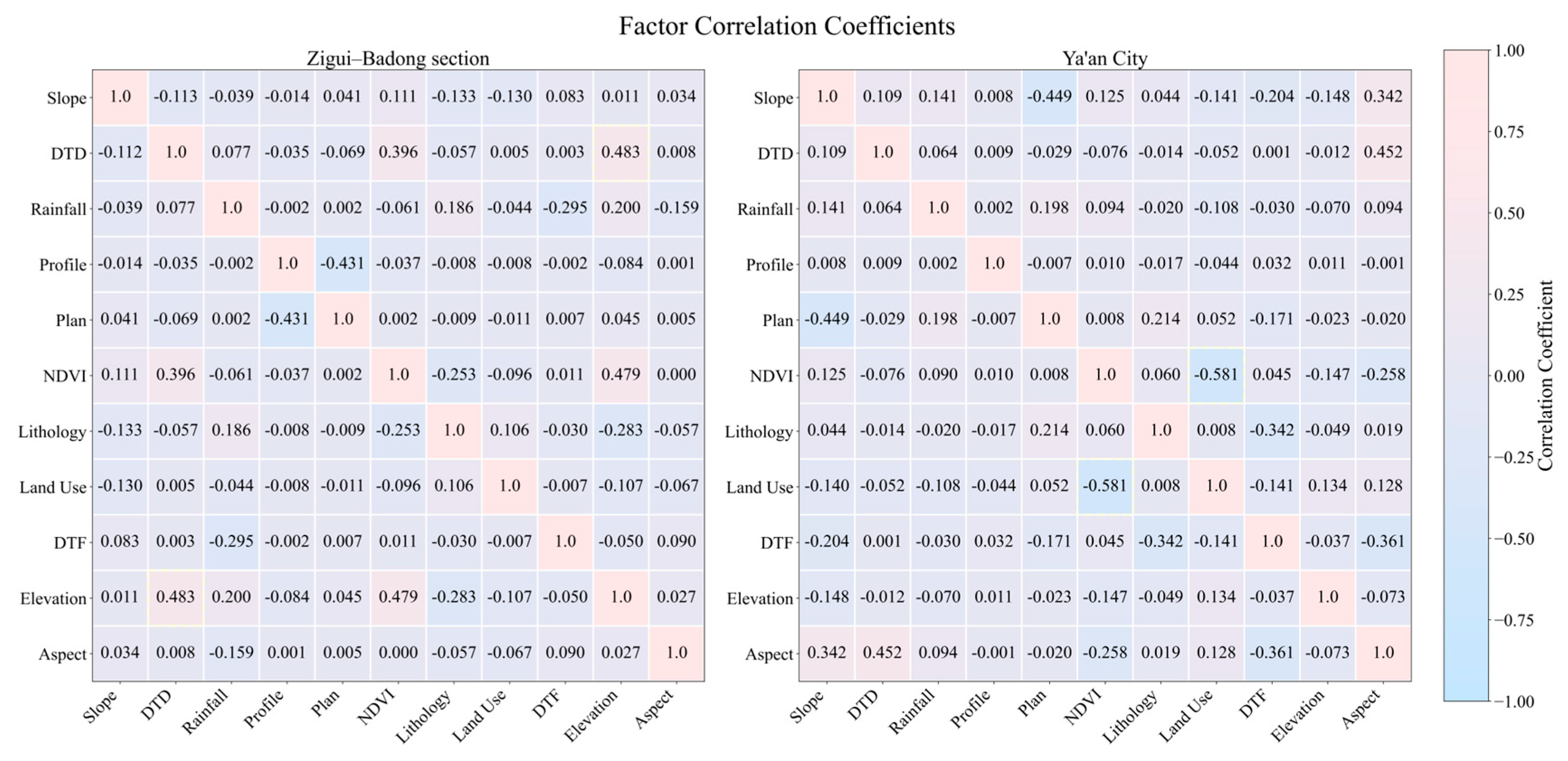
The correlation can be measured using the Spearman correlation coefficient between LCFs [53]. This coefficient is suitable for nonlinear data and calculates the monotonic relationship between variables based on their ranks. Its values range from −1 to +1. The strength of correlation is determined by the absolute value of the coefficient, |q|, and can be categorized as: very strong (0.9–1.0), high (0.7–0.9), moderate (0.4–0.7), low (0.2–0.4), and very weak (0.0–0.2).

2.4.2. Importance Evaluation

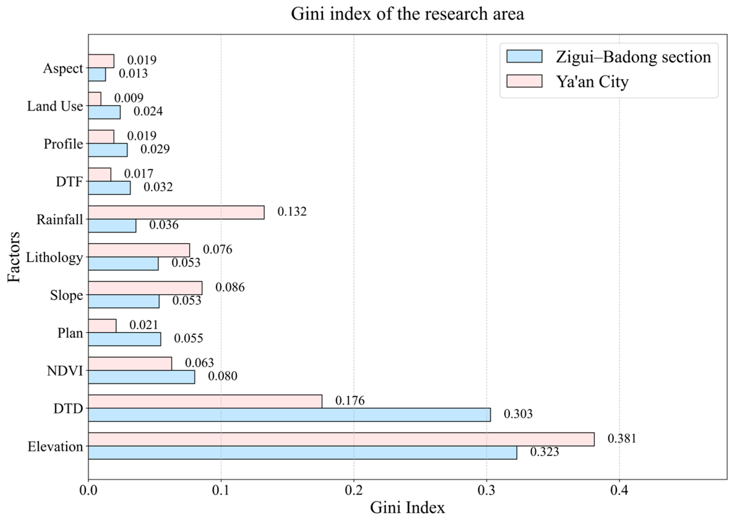
We employ the Gini index to evaluate the importance of LCFs [54]. This method quantifies the importance of each LCF by calculating the average decrease in Gini impurity caused by splits on that factor across all decision trees. A higher importance score indicates a greater contribution of the factor to landslide prediction. The total importance scores of all factors sum to 1, ensuring the comparability and objectivity of the evaluation results.

3. Methods

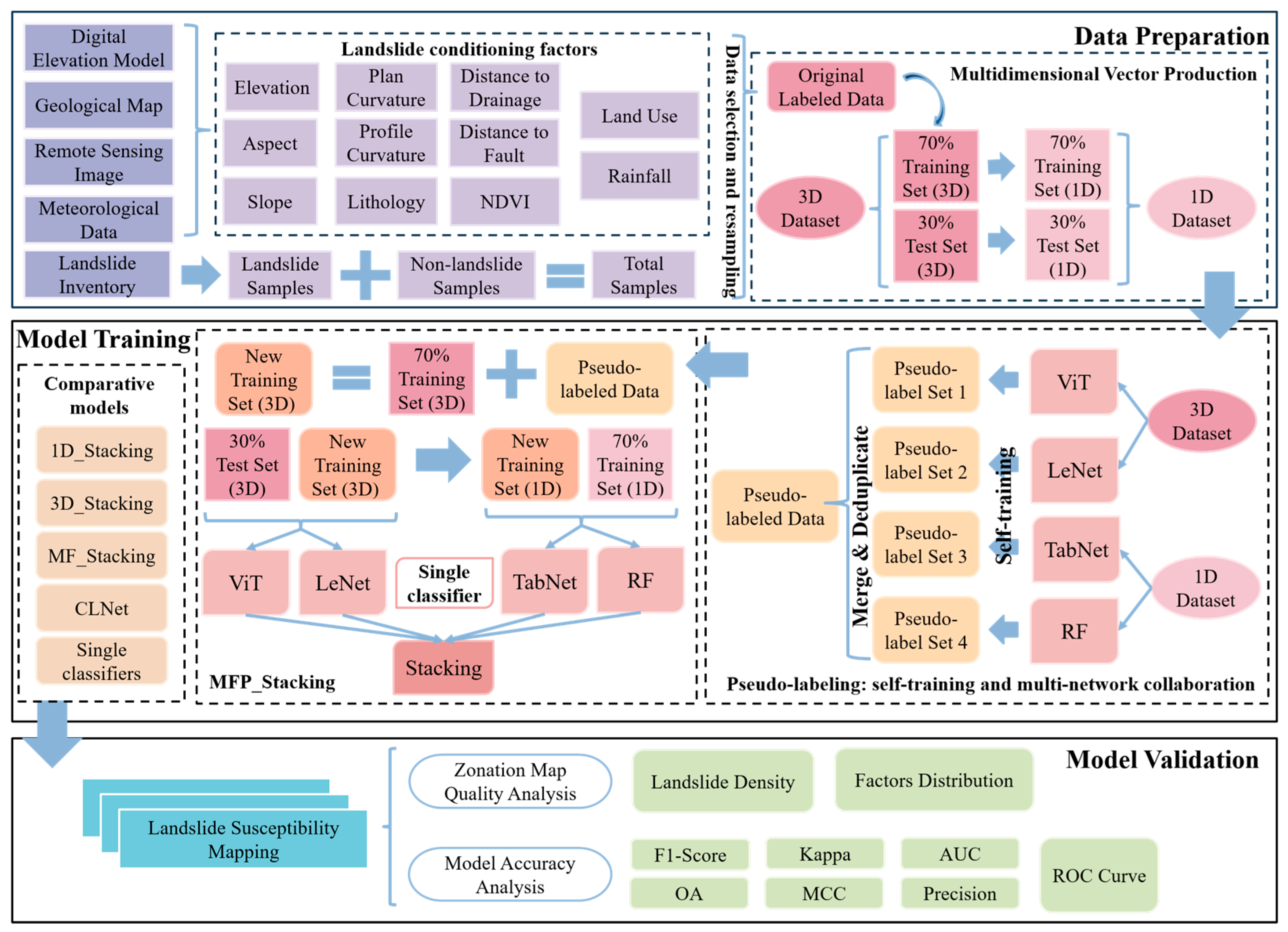
To address the limitations of feature representation in EL models and the challenge of sample scarcity, the MFP_Stacking model is proposed, with its implementation workflow illustrated in Figure 3. It primarily comprises three components: data preparation, model training, and model validation. In the data preparation phase, multidimensional vectors are constructed from historical landslide events and 11 LCFs, establishing the data foundation for model training. In the model training phase, the MFP_Stacking model and comparative models are trained separately using datasets specific to each study area. In the model validation phase, a variety of evaluation metrics, including overall accuracy (OA), the Kappa coefficient, and LD, are employed to assess the performance of the PMF_Stacking model and the comparative models.

3.1. Multidimensional Vector Production

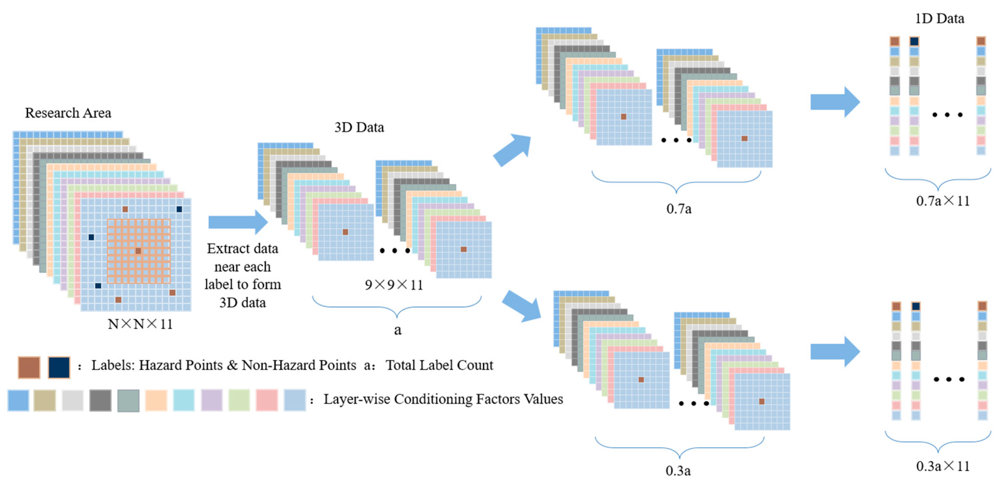
A key challenge of the MFP_Stacking model lies in integrating single classifiers, trained on vectors of different dimensionalities, into the Stacking model. The dataset creation process is shown in Figure 4. During the construction of the Stacking ensemble model, each single classifier must utilize the same training set for each iteration, necessitating standardized preprocessing of the dataset. For the three-dimensional vectors, this study adopts a spatial neighborhood modeling strategy: LCFs are first stacked into a three-dimensional matrix (H, W, C), where H and W represent spatial height and width, respectively, and C denotes the number of LCFs. Then, based on the positional information of positive and negative samples, a local grid window is constructed with each sample point as the center, from which corresponding data is extracted from the three-dimensional matrix. A comparative experiment with multiple-scale windows determines the optimal grid size of 9 × 9, which effectively captures the spatial contextual features of the sample points while minimizing redundant information, resulting in a three-dimensional vector X i 3 D with the shape of (9, 9, 11). Finally, the three-dimensional vectors from all sample points are integrated into the final dataset. Considering that the landslide inventory consists of spatially sparse point samples and the dataset is constructed from these discrete points, the spatial dependence among samples remains within a controllable range. Therefore, the final dataset is randomly divided into training and validation sets at a 7:3 ratio. For the one-dimensional vectors X i 1 D , each is composed of the attribute values of the evaluation factors at the center point of the corresponding three-dimensional vector. The training and validation sets are aligned with those of the three-dimensional dataset to ensure data comparability.
X i 3 D = [ x u , v , c ] u , v = 1 9 , c = 1 11
X i 1 D = X i 3 D h + 1 2 , w + 1 2 , : = [ x i , 1 , x i , 2 , , x i , 11 ]
where x u , v , c denotes the value of the (u,v)-th pixel within a 9 × 9 spatial neighborhood centered on the sample point in the c-th environmental factor layer. h + 1 2   and w + 1 2 represent the central positions of the local window in the row and column directions, respectively, and the colon symbol “:” indicates the extraction of all feature channels.

3.2. Single Classifiers

In this study, RF, TabNet, LeNet, and ViT are selected as the single classifiers for the EL model. RF and TabNet are employed for LSM using one-dimensional vectors. RF is resistant to overfitting and efficiently handles high-dimensional features, while TabNet offers a comparative advantage over other DL models in processing tabular data. The LSM results produced by these two models outperformed those of other machine learning approaches. LeNet and ViT are employed for LSM using three-dimensional vector. LeNet excels at efficiently extracting local features, while ViT offers powerful capabilities in global feature modeling. Their combination facilitates the synergistic optimization of both local and global spatial features. The mechanisms, advantages and limitations, applicable scenarios, and specific roles of all single classifiers are summarized in Table 3.

3.2.1. RF

RF constructs multiple decision trees and combines their predictions through voting to enhance accuracy and robustness [55]. For classification tasks, RF utilizes the full feature set, with each tree making independent predictions for the samples, which are then consolidated by a majority vote. If y ^ k represents the predicted class of the kth tree and C denotes the set of all possible classes, the final RF prediction y ^ is given by:
y ^ = arg m a x c C k = 1 K I y ^ k = c
where I(.) is the indicator function that returns one when the condition is true, and zero otherwise.

3.2.2. TabNet

TabNet captures complex patterns through feature selection and interaction. The model processes data in multiple steps, with each step including an Attentive Transformer, Mask, Feature Transformer, and Split module [56]. The Attentive Transformer uses Sparsemax to generate sparse attention weights and select key features. The Mask module applies a weighting to the input, while the Feature Transformer performs nonlinear transformations on selected features. The Split layer divides the output into two parts: one for prediction and the other for further processing by the attention module. The final prediction is obtained by accumulating the partial results from each step.

3.2.3. LeNet

CNNs are DL models for spatial data, featuring local receptive fields, weight sharing, and hierarchical feature extraction. The local receptive field captures spatial information, allowing neurons to respond to local input patterns. Weight sharing ensures translation invariance and reduces parameters, enhancing model generalization. A typical CNN includes convolutional layers for feature extraction, pooling layers for downsampling, and fully connected layers for prediction [57]. We built a LeNet model based on the LeNet-5 framework, tailored for three-dimensional vector, to perform LSM [58]. The model includes two convolutional layers, two pooling layers, and three fully connected layers.

3.2.4. ViT

The ViT model captures long-range dependencies between any two elements in a sequence through a self-attention mechanism, thereby overcoming the local receptive field limitations of CNNs [59]. The ViT model divides the image into fixed-size patches, linearly maps them into vectors, and augments them with learnable positional embeddings and a class token to retain spatial information and support classification. The input sequence is then processed by multiple Transformer encoder layers, each consisting of a Multi-Head Attention layer and an MLP block. Finally, the output corresponding to the class token is extracted and processed through an MLP head for classification [60]. This study applies the ViT model for LSM, consisting of 11 Transformer encoder layers with 8-head self-attention.

3.3. Stacking Model

Stacking employs a meta-model to combine multiple single classifiers, leveraging their respective strengths while mitigating the shortcomings of individual classifiers, thereby improving the model’s generalization ability and achieving more accurate prediction results [61]. In Stacking, each single classifier is trained independently and makes predictions on the validation set to produce meta-features. The meta-model is then trained using these meta-features to obtain the final prediction.
Assuming there are K single classifiers f 1 , f 2 , f 3 , , f K , and the input sample is x i each single classifier produces a predicted result as follows:
y ^ i ( k ) = f k x i , k = 1,2 , 3 , , K
The outputs of all single classifiers are concatenated to form a meta-feature vector:
Z i = [ y ^ i ( 1 ) , y ^ i ( 2 ) , y ^ i ( 3 ) , , y ^ i ( K ) ]
The meta-model g ( ) performs secondary learning on this vector to obtain the final prediction output:
y ^ i = g ( Z i ) = σ ( k = 1 K w k y ^ i ( k ) + b )
where σ ( ) denotes the Sigmoid function, w k represents the fusion weight learned by the meta-model, and b is the bias term. This formula realizes a weighted nonlinear fusion of the prediction results from different single models, thereby fully leveraging the complementary advantages of each single classifier across different feature spaces.
Finally, for validation data, new samples are first predicted by all single classifiers, and the meta-model subsequently aggregates these predictions to generate the final output [62]. In addition, during the model training phase, cross-validation is utilized to train each base classifier, enhancing the diversity of prediction outcomes and effectively suppressing overfitting.

3.4. Pseudo-Labeling Technique

The pseudo-labeling technique designates unlabeled data with high prediction probabilities as pseudo-labeled data [63], primarily involving two implementation strategies: multi-network optimization and self-training. This study employs a self-training and multi-network collaboration strategy, shown in Figure 5, for pseudo-label generation. Specifically, a set of representative models is first employed for self-training to generate pseudo-labeled samples. The outputs produced by these models are then merged, and duplicate entries are removed based on their spatial coordinates.
During the self-training process, let the original labeled dataset be D L = { ( x i , y i ) } and the unlabeled dataset be D U = { x j } . After training the initial model f θ , the landslide prediction probability of x j is denoted as p j = f θ ( x j ) , where p j [ 0,1 ] , and the non-landslide prediction probability is q j = 1 p j . A staged confidence threshold strategy is then employed for pseudo-label selection, which involves dividing the prediction probability range into S mutually exclusive confidence intervals, denoted as { I s = [ a s , b s ) } s = 1 S , with a specific quota M s assigned to each interval to guide the selection.
The index set of samples within each interval is defined as:
For the positive samples:
J s + = j p j I s .
For the negative samples:
J s = j q j I s = j 1 p j I s
Subsequently, samples are selected from each interval according to the preset quota M s :
For the positive samples:
S s + = M s J s +
For the negative samples:
S s = M s J s
Pseudo-labels are assigned to the selected samples as follows:
y ~ j = 1 , j S s + ;   y ~ j = 0 , j S s
The positive and negative pseudo-labeled samples are merged as
D P i = ( S = 1 S x j , 1 j ϵ S S + ) ( S = 1 S x j , 1 j ϵ S S )
If the same sample is simultaneously selected as both a positive and a negative pseudo-label, it is discarded to avoid label conflicts. The pseudo-labeled dataset D P i is incorporated into the original training set to form an expanded dataset D ' = D L D P i , which is then used for retraining through the following joint loss function:
L total = L L + α t L P = i D L y i log f θ x i α t j D P y ~ j log f θ x j
where α ( t ) denotes a dynamically adjusted weighting coefficient at iteration step t , which controls the influence of pseudo-labeled samples on the overall loss. Finally, iterative optimization is performed through alternating updates until convergence [64]. Through the above self-training process, the m models each generated their own pseudo-labeled dataset D p i . These datasets were merged and deduplicated based on spatial coordinates, ultimately yielding the complete pseudo-labeled dataset D P .
The confidence intervals in the staged confidence threshold strategy used in this paper are partitioned according to the approximate ranges of the landslide susceptibility levels. The segmented confidence threshold strategy divides the model’s predicted confidence scores according to the approximate ranges of landslide susceptibility levels and selects pseudo-labels at different ratios for each interval. The interval (1.0–0.8) corresponds to the very high susceptibility zone, containing samples in which the model is most confident; the interval (0.8–0.6) corresponds to the high susceptibility zone, containing samples in which the model is relatively confident; and the interval (0.6–0.4) corresponds to the moderate susceptibility zone, containing samples for which the model is relatively uncertain but still includes potentially valuable information. This strategy prevents the overconfidence issue that arises when only the highest-confidence samples are selected. In experiments, if only samples with the highest predicted confidence (>0.8) are selected as pseudo-labels, these samples become highly concentrated in the very high susceptibility zone. Although this can improve classification accuracy in high-risk areas in the short term, from the perspective of susceptibility mapping, it unreasonably enlarges the predicted area of the very high susceptibility zone while neglecting boundary delineation for moderate and high susceptibility zones, ultimately degrading the quality of the generated susceptibility map. This phenomenon was verified in the ablation experiments conducted in this study.
In addition, to ensure the quality of pseudo-labels generated during training, we calculated the average confidence W of the pseudo-labels to reflect the overall reliability of the pseudo-labeled dataset. A two-sample Kolmogorov–Smirnov (KS) test [65] was then performed to assess whether the distributions of landslide-related factor feature in the original labeled dataset (a total of m samples) and the pseudo-labeled dataset (a total of n samples) are consistent. This test statistically compares the two samples by computing the maximum vertical distance D m , n between their empirical cumulative distribution functions (ECDFs). The null hypothesis H 0 assumes that D P and D L are drawn from the same continuous distribution, while the alternative hypothesis H 1 assumes that they are drawn from different distributions. Under the null hypothesis, when the sample sizes m and n are sufficiently large and tend to infinity, the statistic m n m + n D m , n converges in distribution to the Kolmogorov distribution. Based on this, the p -value corresponding to the observed D m , n can be calculated. In this study, the KS test was conducted for each continuous factor, and the corresponding p -values were recorded, with the final average denoted as m e a n _ p . At a significance level of α = 0.05 , if m e a n _ p > 0.05 , the null hypothesis H 0 is not rejected, indicating no significant difference between the distributions of the two datasets.
W = ( p 1 + p 2 + p 3 + + p n ) n
D m , n = s u p t | F m ( t ) G n ( t ) |
where sup denotes the supremum (representing the maximum absolute difference over all possible values of t), F m ( t ) is the ECDF of the original labeled dataset, and F n ( t ) is the ECDF of the pseudo-labeled dataset.

3.5. MFP_Stacking

The Stacking model (MFP_Stacking), based on multidimensional feature collaboration and pseudo-labeling techniques, primarily consists of two components: multidimensional feature collaborative modeling and pseudo-label augmentation.

3.5.1. Multidimensional Feature Collaborative Modeling

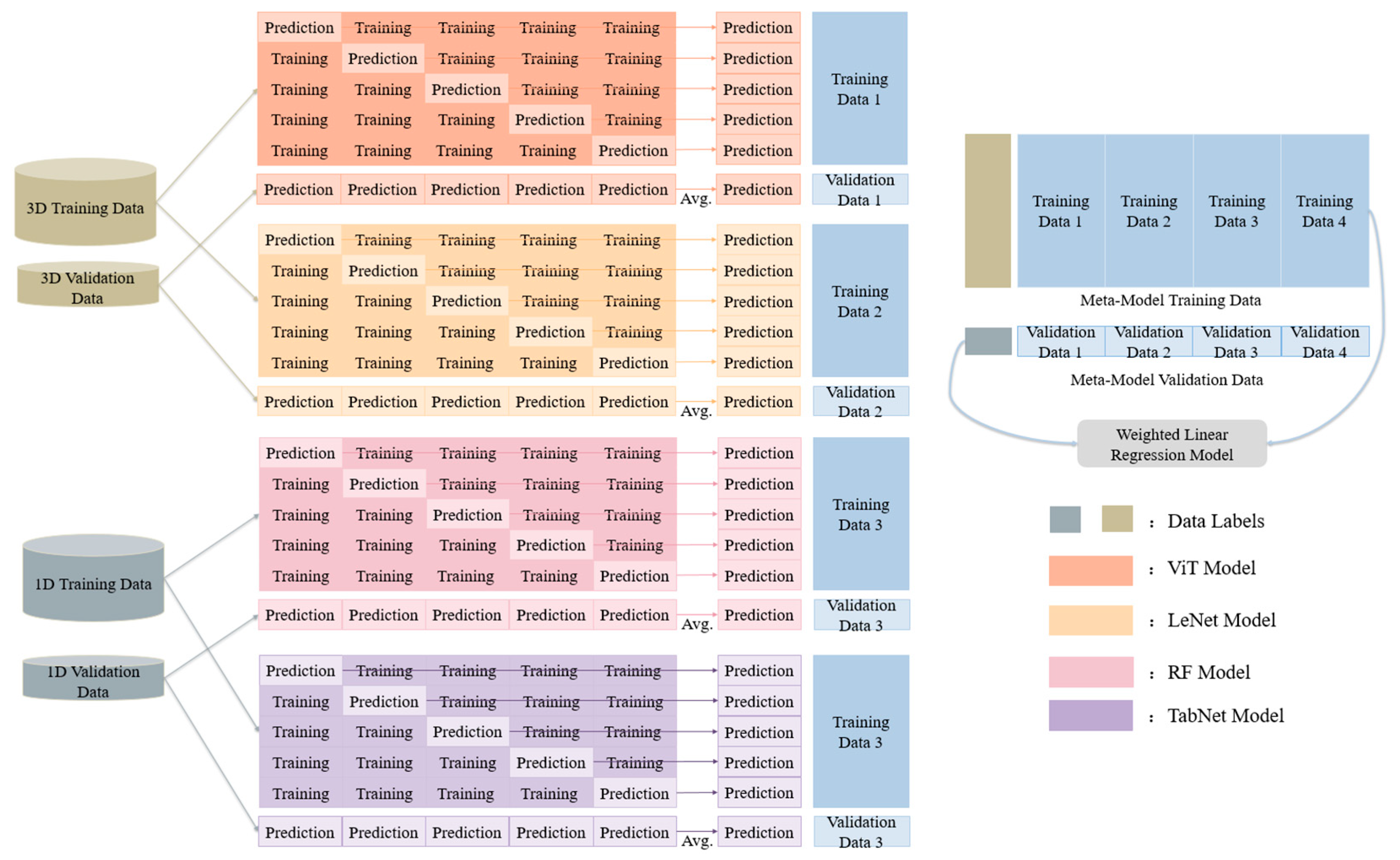
To overcome the limitations of feature representation in EL models, a multidimensional feature collaborative modeling strategy based on the Stacking model and multidimensional feature vectors is proposed. The model framework is illustrated in Figure 6. Specifically, in the Stacking model, TabNet, RF, LeNet, and ViT are employed as the single classifiers, denoted as f R F , f T a b N e t , f L e N e t , and f V i T , respectively. First, the one-dimensional and three-dimensional vectors are fed into the corresponding types of single classifiers to obtain their landslide probability predictions:
p R F = f R F X i 1 D , p T a b N e t = f T a b N e t X i 1 D , p L e N e t = f L e N e t X i 3 D , p V i T = f V i T X i 3 D
Next, the outputs of the four single classifiers are concatenated to form the meta-feature vector:
h =   p R F ,   p T a b N e t ,   p L e N e t ,   p V i T  
Finally, a weighted linear regression model is adopted as the meta-model to produce the final prediction probability:
p ^ = σ w h + b
where w = [ w 1 , w 2 , w 3 , w 4 ] denotes the learnable weight vector, b is the bias term, and σ represents the activation function.
In this modeling strategy, TabNet and RF are responsible for extracting global statistical attributes from one-dimensional vectors (one-dimensional features). Such features (e.g., elevation, slope, and lithology) characterize the static properties of sampling points and effectively depict fundamental predisposing conditions for landslide occurrence, including lithological weakness and slope steepness. LeNet and ViT, respectively, extract local spatial morphological features and global spatial topological correlation features from three-dimensional vectors (two-dimensional spatial neighborhood multi-channel features). These spatial features capture key spatial structural information such as landform morphology, surface curvature, and hydrological connectivity, thereby reflecting triggering mechanisms of landslides, including rainfall accumulation and stress distribution within slopes. Finally, a meta-model is used to integrate the multidimensional information, enabling the collaborative modeling of spatial and non-spatial features. Essentially, this strategy integrates the statistical patterns of conditioning factors with the spatial structural characteristics controlling hazard development, thereby enabling the model to more comprehensively simulate the multi-scale geological processes that underpin landslide occurrence. By leveraging the strengths of each single classifier and forming effective complementarity across scales and feature structures, the proposed strategy substantially enhances the model’s representational capacity and predictive performance.

3.5.2. Pseudo-Label Augmentation

To mitigate the impact of sample scarcity on model performance, we innovatively incorporate pseudo-labeling techniques into the Stacking model. The generated pseudo-labels were introduced solely into the training set for model training and were strictly excluded from the independent validation set to ensure the purity of the validation data. In this study, in light of the tendency of single models to produce overly concentrated pseudo-label feature distributions, thereby overlooking minority class features, a self-training and multi-network collaboration strategy is employed for pseudo-label selection. The single classifiers within the Stacking model (LeNet, ViT, TabNet, and RF) are employed as pseudo-label generators to ensure diversity in feature distributions. The integrated pseudo-labeled and original labeled data are combined to form an augmented training set, employed to train the Stacking model.

3.6. Model Evaluation Measures

We adopt a diverse array of performance evaluation metrics to comprehensively assess the effectiveness and reliability of the model, including OA, kappa coefficient, precision, recall, F1-score, Matthews correlation coefficient (MCC), receiver operating characteristic (ROC) curve, and area under the curve (AUC). These metrics reflect the model’s predictive capability from multiple perspectives, ensuring the comprehensiveness and scientific rigor of the evaluation.
O A = T P + T N T P + T N + F P + F N
k = p o p e 1 p e
P r e c i s i o n = T P T P + F P
R e c a l l = T P T P + F N
F 1 = 2 · P r e c i s i o n · R e c a l l P r e c i s i o n + R e c a l l
M C C = T P × T N F P × F N ( T P + F P ) ( T P + F N ) ( T N + F P ) ( T N + F N )
T P R = T P T P + F N , F P R = F P F P + T N
In the equations, TP denotes the number of samples correctly predicted as landslides, TN represents the number of samples correctly predicted as non-landslides, FP refers to the number of samples incorrectly predicted as landslides, and FN indicates the number of samples incorrectly predicted as non-landslides. p o represents the proportion of agreement between the model predictions and the actual labels, while p e denotes the expected agreement by chance under random label assignment.
In addition, to evaluate the quality of landslide susceptibility zonation maps generated by different models, it is necessary to calculate the proportion of each susceptibility level area relative to the total study area (PC), the proportion of historical landslides occurring within each susceptibility level (PL), and the LD. These metrics quantify the likelihood of landslide occurrence within different susceptibility zones.
L D = P L P C

4. Results

4.1. Analysis of the LCFs

The results of Spearman correlation analysis, as shown in Figure 7, indicate generally weak inter-factor correlations across both study areas, with the highest coefficients being 0.483 and −0.581, respectively, within the moderate correlation range. This assessment of factor importance, illustrated in Figure 8, further demonstrates that all factors contribute to landslide prediction. Given the insignificant correlations among factors and their collective predictive value, all 11 LCFs were retained for LSM.

4.2. Model Parameter Settings

All experiments in this study were implemented using Python 3.6 and executed on a Linux-based operating system. The hardware platform had an Intel Xeon Silver 4210R processor, 20 GB of RAM, and an NVIDIA GeForce RTX 3090 GPU. During model training, a global grid search strategy is employed for hyperparameter optimization to obtain the best model performance. The number of search iterations is determined by the range and step size of each parameter, with the detailed configurations summarized in Table 4. Table 5 provides detailed parameter configurations for the MFP_Stacking, 1D_Stacking, 2D_Stacking, MF_Stacking, TabNet, RF, LeNet, and ViT models, along with the single classifiers’ composition and meta-model selection for each EL model.

4.3. Comparison of LSM Results

We design comparative experiments from the following four perspectives to validate the effectiveness of the proposed model. First, independent prediction results from each single classifier were generated and compared with the ensemble output to validate the effectiveness of the EL models. Second, an MP_Stacking model was constructed by removing the pseudo-labeling component from the MFP_Stacking model, and its results were compared with those of the full model to assess the performance gains attributable to the pseudo-labeling technique. Third, stacking models based solely on one-dimensional features and two-dimensional spatial neighborhood multi-channel features (1D_Stacking and 2D_Stacking) were developed and compared with the MF_Stacking model to evaluate the benefits of the proposed multidimensional feature representation strategy. Finally, to further validate the competitiveness of the MFP_Stacking model relative to more advanced DL architectures, we conducted a supplementary comparison experiment using a recently high-performing CNN–Transformer hybrid model (CLNet). In this model, local spatial features are first extracted via a CNN module (three convolutional layers), after which the learned representations are fed into a Vision Transformer encoder—comprising 11 layers, each utilizing an 8-head self-attention mechanism—to capture global contextual dependencies, ultimately yielding the final susceptibility predictions.
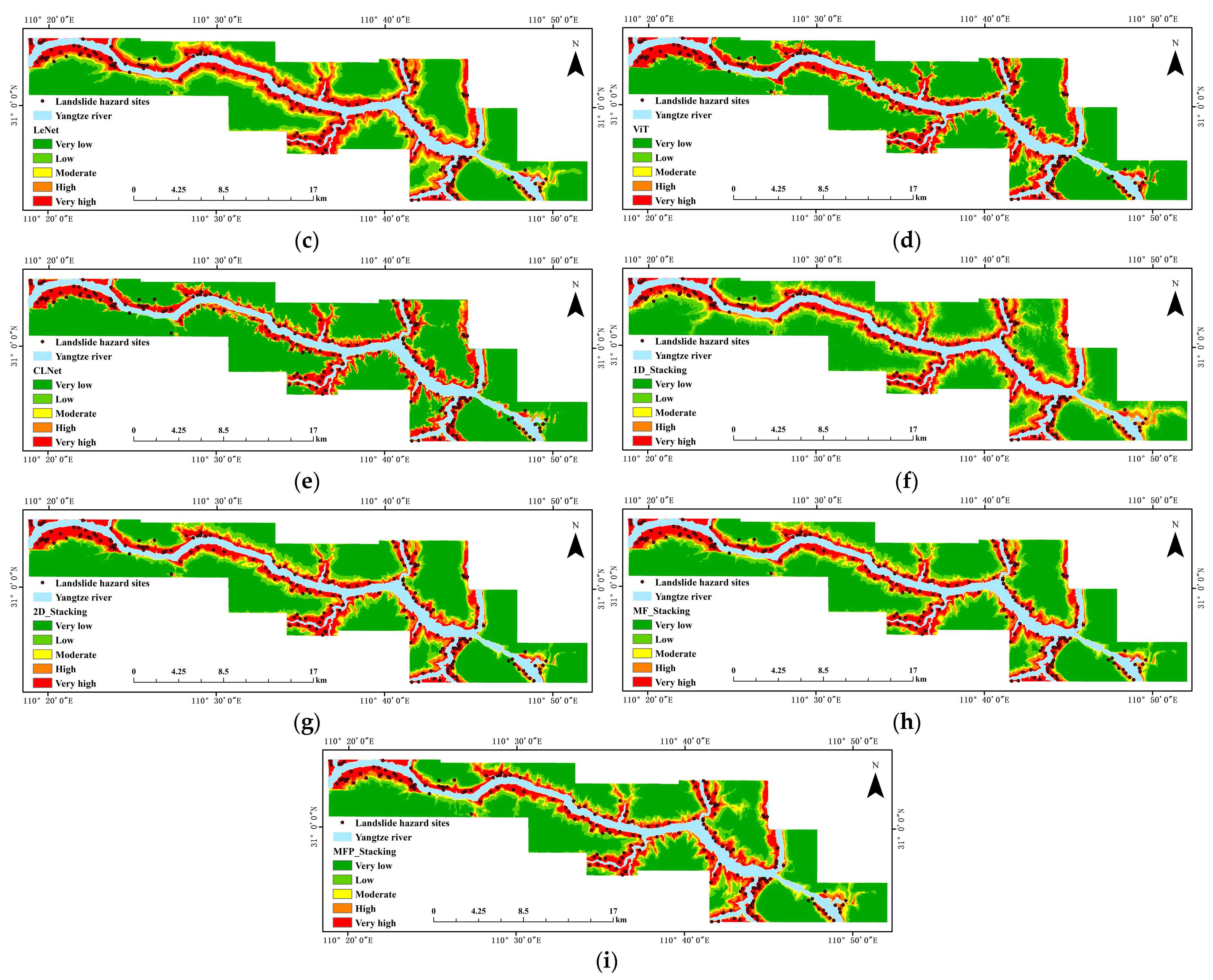
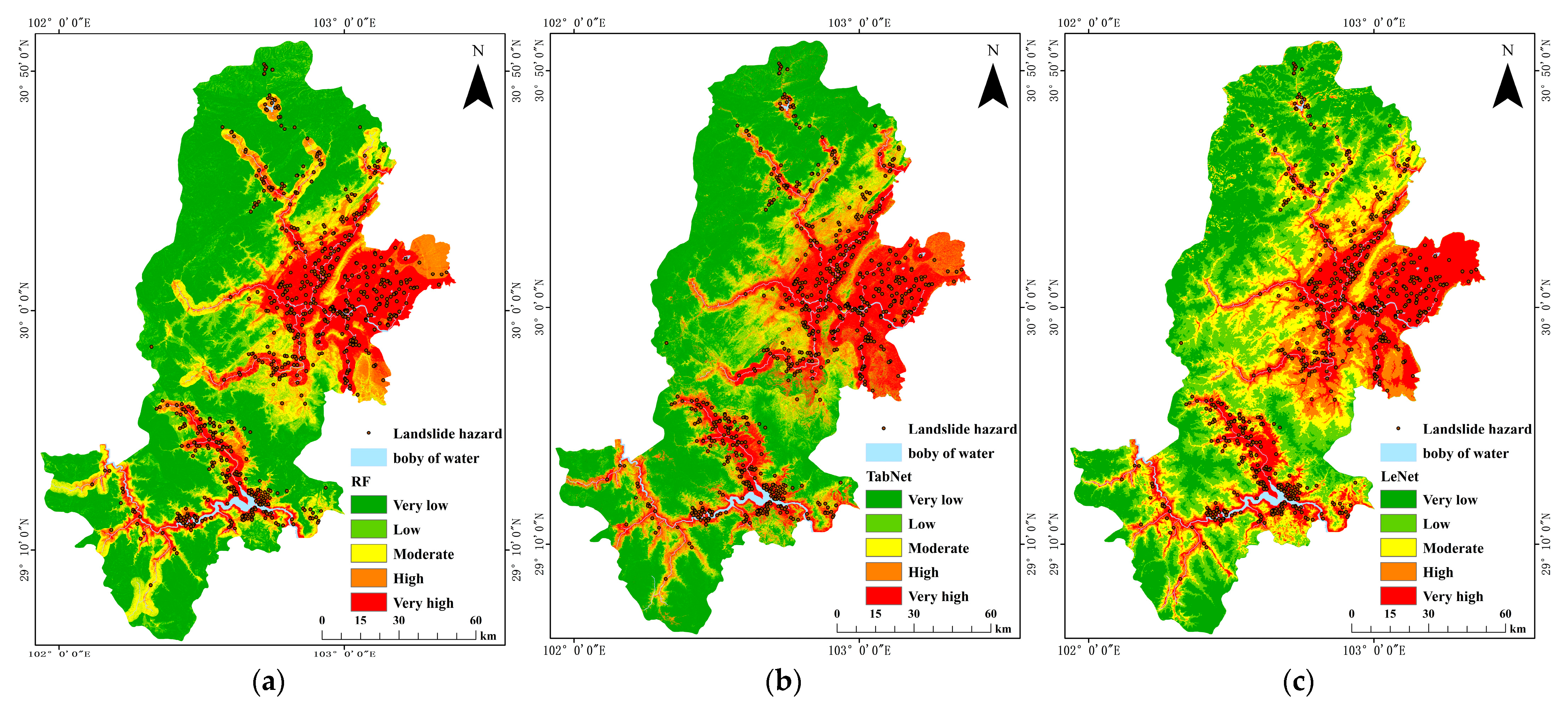
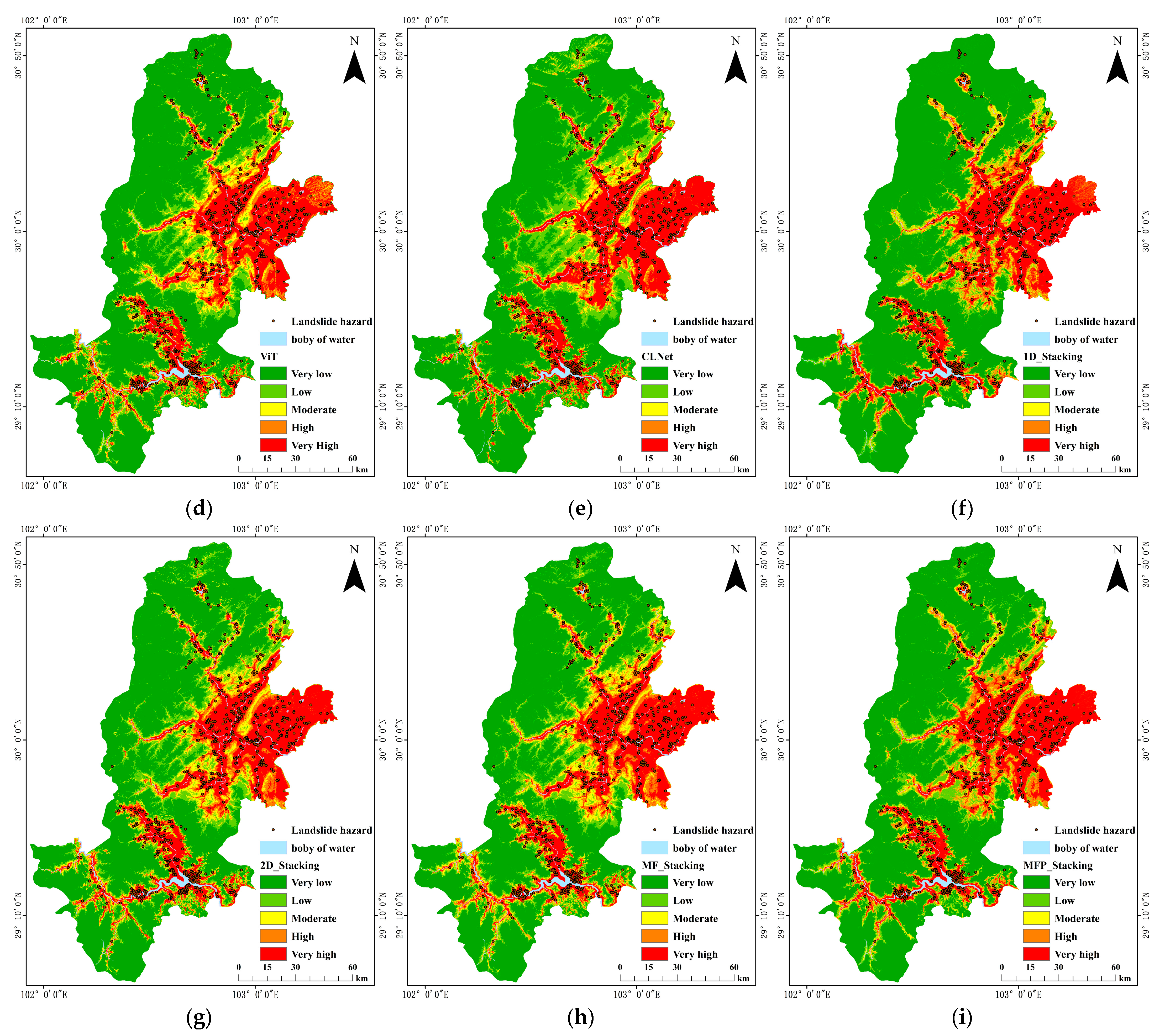
First, LSM is performed using the MFP_Stacking model and other comparative models. The landslide probability values from each model are then classified into five susceptibility levels, very low, low, moderate, high, and very high, using the natural breaks method to generate susceptibility zonation maps. The results of the landslide susceptibility zonation maps for each study area are shown in Figure 9 and Figure 10. The analysis reveals strong spatial consistency between the high to very high susceptibility zones and historical landslide distributions, with clear clustering patterns. Specifically, in the Zigui–Badong section, these zones are mainly located along both banks of the Yangtze River, whereas in Ya’an City, they are concentrated in the Qingyi River basin, nearby lakes, and eastern low-elevation hills.
To evaluate the quality of landslide susceptibility zonation maps generated by different models, we calculated the PC, PL, and LD values, as summarized in Table 6. In both study areas, the LD across different susceptibility levels shows a consistent increasing trend with rising susceptibility, indicating that each model effectively captures the spatial characteristics of landslide distribution, and that the resulting susceptibility zonation maps align well with the classification criteria. A comparative analysis of PC, PL, and LD indicators reveals that the MFP_Stacking model performs best in the very low to low susceptibility zones. In the Zigui–Badong section, the low to very low susceptibility zones account for 67% of the area but only 1% of the landslides, with an LD of 0.04. In Ya’an City, these zones cover 64% of the area, contain 3% of the landslides, and exhibit an LD of 0.24. This phenomenon suggests that the model is able to achieve a lower LD in the region while covering a larger proportion of the area. Within the high to very high susceptibility zones, the MFP_Stacking model exhibits remarkable performance. In the Zigui to Badong section, the area proportion is 25%, with a landslide proportion of 97% and an LD of 6.5; in Ya’an City, the area proportion is 30%, the landslide proportion is 93%, and the LD is 5.1. This phenomenon indicates that the model can encompass the majority of landslides within a smaller area fraction, while achieving the highest LD in the region. The results demonstrate that the MFP_Stacking model exhibits superior learning capability and predictive performance.
A comparison among the learning outcomes of 1D_Stacking, 2D_Stacking, and individual classifiers reveals that ensemble models effectively integrate the strengths of single models, balance the area proportions and spatial distribution of landslide susceptibility zones, and consequently achieve more stable learning performance. A comparison of susceptibility maps derived from one-dimensional features (RF, TabNet, 1D_Stacking) and two-dimensional spatial neighborhood features (LeNet, ViT, 2D_Stacking) reveals that the former yields relatively scattered results with insufficient spatial coherence, reflecting its focus on point-based statistical regularities, whereas the latter exhibits higher spatial continuity, enabling the identification of landslide clusters and highlighting its advantage in capturing overall spatial characteristics. A comparison of the learning results between MF_Stacking and both 1D_Stacking and 2D_Stacking reveals that MF_Stacking demonstrates improved performance across all susceptibility zones, validating the effectiveness of multidimensional feature collaborative modeling in producing higher-quality landslide susceptibility zonation maps. Moreover, a comparative analysis between MFP_Stacking and MF_Stacking indicates that, under similar area proportions, MFP_Stacking achieves lower LD in the very low to low susceptibility zones and higher density in the high to very high zones of the Zigui–Badong section; likewise, compared to MF_Stacking, MFP_Stacking attains higher LD in the high to very high susceptibility zones of Ya’an City. These results confirm the effectiveness of the pseudo-labeling technique in enhancing the predictive accuracy of LSM. Finally, comparison of the susceptibility maps generated by CLNet, LeNet, and ViT indicates that the fusion of local and global features in CLNet leads to higher spatial coherence and improved overall map quality. However, its performance remains inferior compared to the MF_Stacking and MFP_Stacking models proposed in this study, which fully demonstrates the superior capability of our method in capturing critical attributes and spatial characteristics.

4.4. Model Performance Evaluation

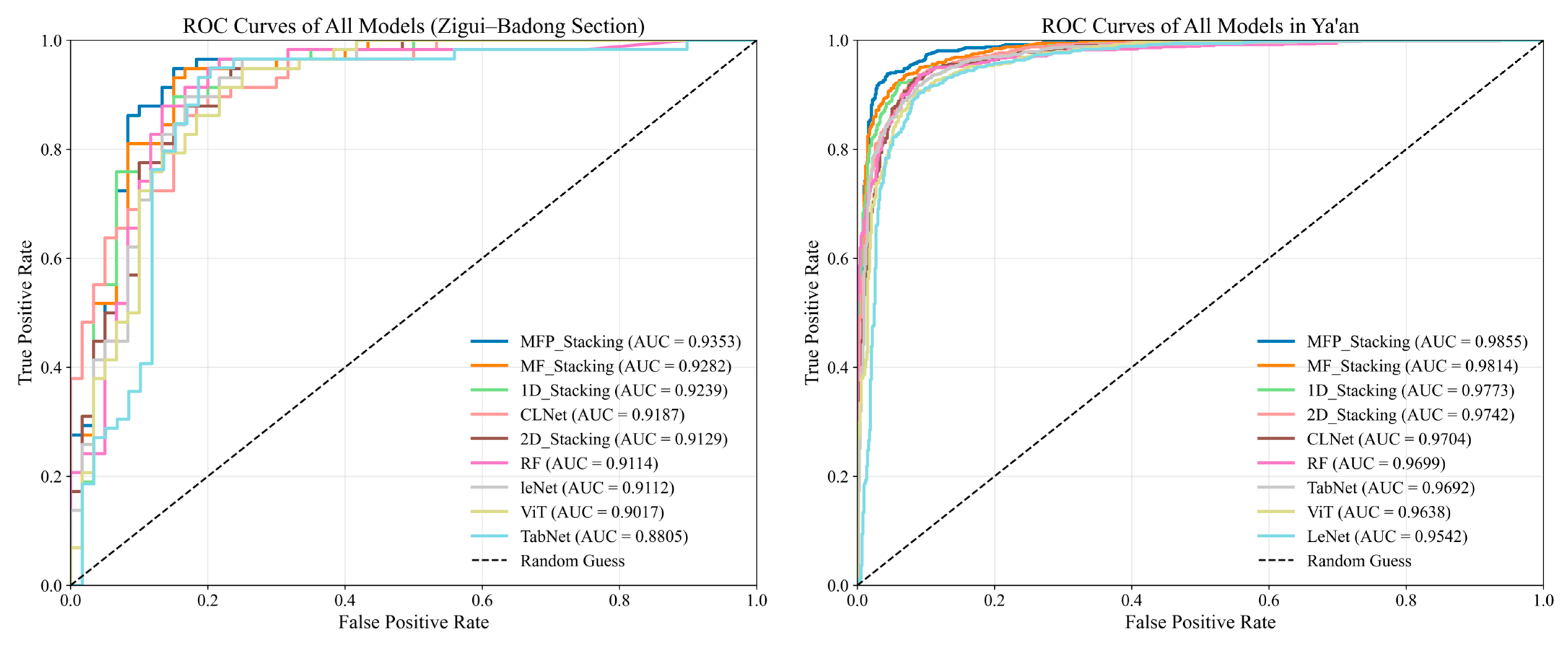
Based on the evaluation metrics of the validation sets across different models presented in Table 7, as well as the ROC curves shown in Figure 11, the MFP_Stacking model consistently outperformed all comparative models across every metric. Specifically, it achieved an overall performance improvement of 2.4% in the Zigui–Badong section and 2.0% in Ya’an City. Moreover, it recorded the highest AUC values of 0.9353 and 0.9855 in the respective regions, further underscoring its remarkable predictive capability.
A comprehensive analysis of the performance metrics shows that the 1D_Stacking model outperforms TabNet across all evaluation indicators in the Zigui–Badong section and achieves an average improvement of 0.8% over the base classifiers in Ya’an City. Compared with LeNet and ViT, the 2D_Stacking model demonstrates an average improvement of 1.8% across all metrics in the Zigui–Badong section and 1.9% in Ya’an City. The analysis of the landslide susceptibility maps further demonstrates that the EL model effectively amalgamates the strengths of individual models, thereby compensating for the limitations inherent in single model.
The MF_Stacking model exhibits an average improvement of 1.8% across all metrics in the Zigui–Badong section and 1.0% in Ya’an City compared to the 1D_Stacking and 2D_Stacking models. A comprehensive analysis of the MF_Stacking model’s accuracy and susceptibility map performance indicates that the improvement in model performance is primarily attributable to its ability to collaboratively characterize landslide development mechanisms across multiple dimensions. Specifically, the model employs global attention combined with local convolutional perception to capture the spatial patterns of geological factors such as lithology, faults, and fluvial erosion, while simultaneously utilizing one-dimensional factors to obtain quantitative statistical attributes, thereby enhancing its capacity for comprehensive interpretation of complex geological environments. Taking the Zigui–Badong section as an example, two-dimensional multi-channel spatial neighborhood features enable the identification of continuous slope variations along both banks of the Yangtze River, whereas one-dimensional features emphasize the statistical significance of slope factors at the pixel scale. The synergy of these two feature dimensions allows the model to identify not only “landslide-prone points” but also “landslide-prone belts,” producing susceptibility maps whose spatial distribution aligns more closely with historical landslide records.
Compared to the MF_Stacking model, the MFP_Stacking model achieves an average improvement of 1.4% across all metrics in the Zigui–Badong section and 1.0% in Ya’an City, indicating that pseudo-labeling effectively mitigates the limitations caused by insufficient labeled data and enhances the model’s overall performance. This result directly addresses the critical challenge of applying advanced machine learning models in data-scarce regions, a pervasive issue in large-scale and regional LSM. In both the Zigui–Badong and Ya’an study areas, the inherently limited availability of labeled samples, compounded by the constraints of N-fold cross-validation, exemplifies such data-constrained conditions. The performance improvement of MFP_Stacking over MF_Stacking thus serves as direct empirical evidence for the applicability and robustness of the pseudo-labeling technique in environments where high-quality labeled inventory data are scarce, thereby underscoring its potential in real-world disaster prevention efforts.
Finally, the comparative analysis of LeNet, ViT, CLNet, MF_Stacking, and MFP_Stacking shows that, although CLNet achieves an average improvement of 1.7% across various evaluation metrics compared with the baseline DL models—demonstrating its competitiveness as a recently high-performing model—both MF_Stacking and MFP_Stacking still attain higher accuracy and produce susceptibility maps of superior quality. These results confirm the superiority of our proposed hybrid strategy. The improvements observed in CLNet are mainly attributed to optimizations within its DL framework, whereas the higher performance of the MF_Stacking and MFP_Stacking models results from the integration of multidimensional feature collaboration and pseudo-label enhancement beyond the architectural level, enabling more pronounced performance gains than those achieved by a pure DL framework.

5. Discussion

5.1. Model Complexity and Its Practical Implications

5.1.1. The Substantive Significance of Performance Gains in Early Warning Applications

The MFP_Stacking model demonstrates performance gains over simpler models on the overall evaluation metrics, showing improvements of approximately 2.0% and 2.4%, respectively. This enhancement holds substantive significance for geohazard early warning and national spatial planning. The core requirement of geohazard early warning is to capture the vast majority of potential landslide locations within the smallest possible area. This necessitates that the model not only achieves high accuracy but also possesses an extremely high Risk Concentration (LD) and Landslide Coverage (PL). Analyzing the quality of the zonation map, the MFP_Stacking model successfully concentrated 97% of historical landslides within the high- to extremely high-risk zones, which collectively cover only 25% of the study area in the Zigui-Badong section. Its LD is significantly higher than that of the contrasting models. Similarly, in Ya’an City, the model concentrated 93% of the landslides within the 30% high-risk area. This result demonstrates that the improvement in OA manifests in the zoning map as a reduction in the area of high-risk zones and an increase in risk concentration. In practical application, this implies the ability to achieve maximized coverage and monitoring of virtually all potential hazard points with lower disaster prevention cost and land use restrictions, thereby enhancing the reliability and efficiency of the early warning system.

5.1.2. Model Complexity

Table 8 reflects the parameter count and computational efficiency of each base model. The learning process of the EL models discussed in this paper is based on combining the training of these single classifiers. Given the available computational resources, parallel processing was chosen; hence, their fundamental computational efficiency is similar to that of the respective single classifiers. However, when evaluating the overall computational complexity of the MFP_Stacking model, two primary factors need to be considered: Firstly, the N-fold cross-validation mechanism leads to an inference time that is N times that of a single classifier. Second, the MFP_Stacking model incurs additional time overhead during the pseudo-label selection phase, though this duration is difficult to calculate precisely.
Overall, the computational complexity of the MFP_Stacking model is significantly higher than that of the base models, yet it is precisely this elevated complexity that drives its improved performance. This ensemble strategy not only effectively overcomes the limitations of feature representation in pure DL models for LSM tasks but also, to some extent, alleviates the issue of sample scarcity. Therefore, the performance gain achieved through this increase in computational complexity is not merely a numerical enhancement in model evaluation metrics; rather, it allows the model to more accurately capture and separate nonlinear relationships within complex geological processes, improving the model’s generalization capability to geological environmental changes. This, in turn, ensures the scientific validity and high confidence of the landslide susceptibility zonation results.

5.2. Visualization of an LSM for the Proposed Model

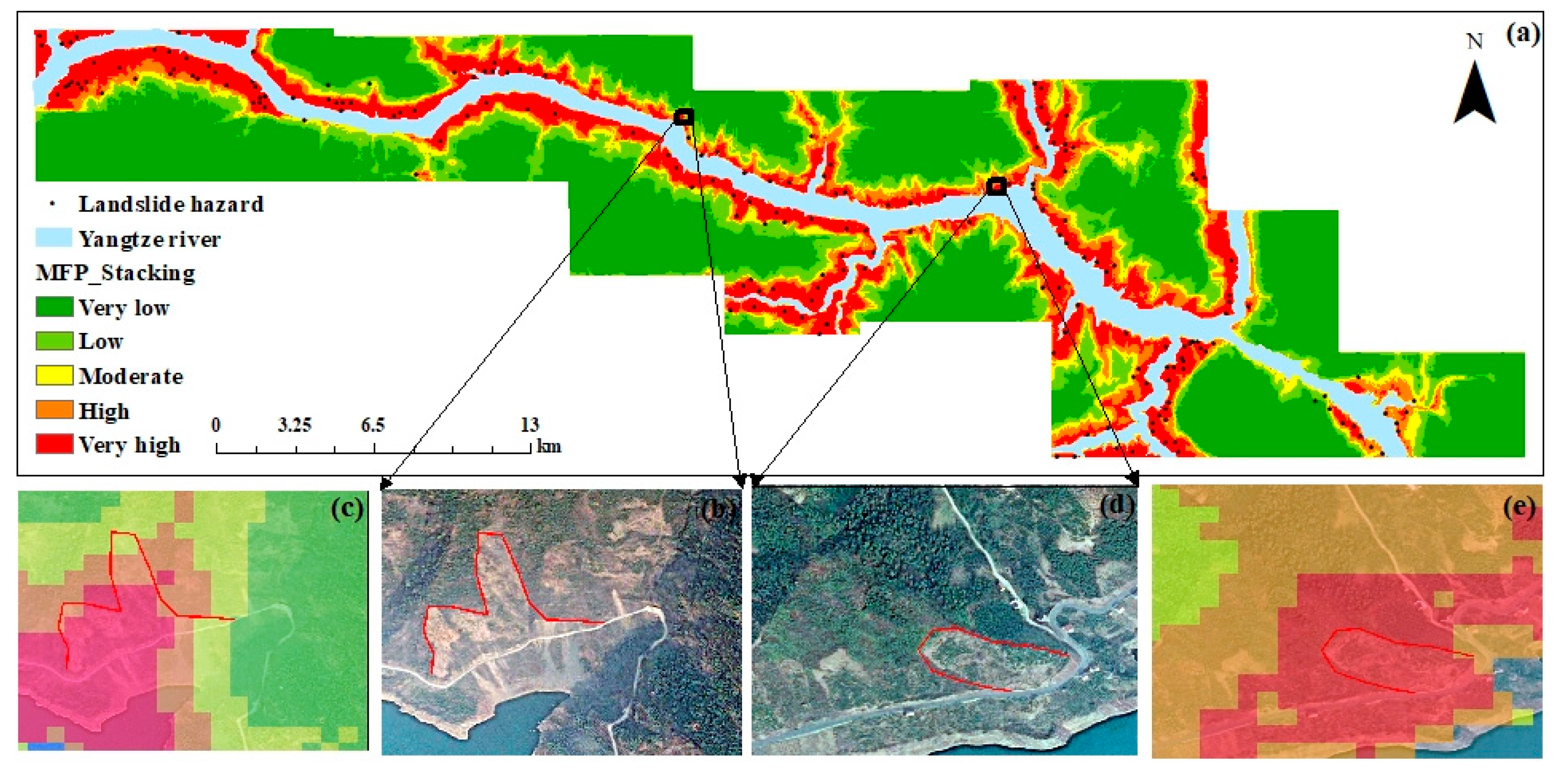
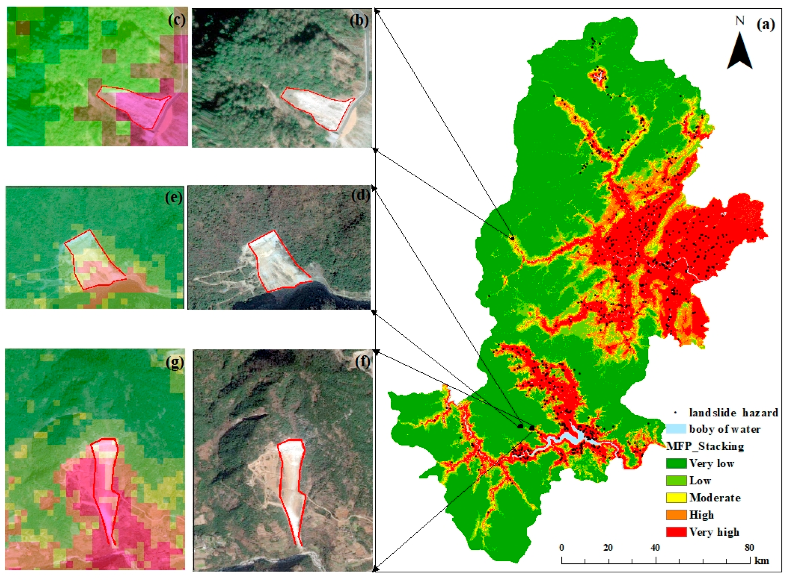
Figure 12 and Figure 13, respectively, display the World Imagery high-resolution satellite basemaps and the corresponding susceptibility zonation maps of the two study areas. Figure 12b,d and Figure 13b,d,f highlight landslide images outside the training labels within each study area, while Figure 12c,e and Figure 13c,e,g show the predicted susceptibility zones corresponding to these landslide images. These images reveal a substantial concordance between the actual landslides and the very-high- to high-susceptibility zones. This not only highlights the model’s outstanding generalization ability but also substantiates its effectiveness in identifying potential landslide-prone areas under real-world conditions. This result demonstrates that our model effectively captures the critical geological, topographic, and other environmental factors influencing landslide occurrence, thereby enabling the spatial prediction of unknown landslides. Moreover, the favorable performance across multiple study areas further reflects the proposed model’s strong regional adaptability and stability. Collectively, these visualization results provide practical confirmation of the MFP_Stacking model’s reliability and practical value in regional landslide susceptibility assessment.

5.3. Model Stability Analysis

To evaluate the sensitivity of each EL model to sample proportions, we systematically adjusted the ratio between the training and validation sets (ranging from 10% to 90%) for LSM and obtained the corresponding AUC validation results under different sample proportions, as shown in Table 9. The results indicate that the EL models consistently outperform single classifiers across all sample ratios and maintain robust predictive performance even under limited landslide samples. Among them, MF_Stacking consistently surpasses both 1D_Stacking and 2D_Stacking across all ratios, demonstrating superior robustness. In addition, to assess whether the differences in AUC values under varying training set proportions were statistically significant, pairwise comparisons were performed using the DeLong test. This nonparametric test is widely employed to evaluate differences between correlated ROC curves, with a significance level of α = 0.05. Differences were considered statistically significant when p < 0.05. The results indicate that AUC differences were significant for training set proportions between 10% and 40%, whereas differences between 50% and 90% were not significant due to the high similarity and minimal fluctuation of AUC values. This suggests that model performance improves rapidly at low training set proportions but stabilizes when the training set exceeds approximately 60%.
In addition, to investigate how the allocation ratios and generation quantities of pseudo-labeled samples within different confidence intervals affect model performance, we systematically designed and conducted a series of experiments. By varying the sample proportions across the confidence intervals (1–0.8, 0.8–0.6, 0.6–0.4) and controlling the total number of pseudo-labels, we assessed the effects of different parameter combinations on the model’s AUC values, as detailed in Table 10. The experimental results demonstrate that the distribution ratio of pseudo-labels has a significant impact on model performance. When only high-confidence samples are used (with a ratio of 1:0:0), the AUC value reaches its maximum; however, this also expands the areal proportion of high and very-high susceptibility zones, thereby diminishing the overall quality of the susceptibility map. In contrast, incorporating a certain proportion of medium- and low-confidence samples (with a ratio of 6:3:1) yields superior results, indicating that a well-balanced configuration of multi-level confidence samples enhances the model’s generalization ability and robustness. Moreover, the number of pseudo-labels also needs to be moderate: too few cannot fully exploit the information of unlabeled samples, while too many may introduce noise and degrade model performance.
A systematic comparison of AUC performance under different parameter combinations revealed that, in the Ya’an region, the optimal confidence ratio was 6:3:1, and a pseudo-label selection strategy of 200 × 4 yielded a total of 550 high-quality pseudo-labels. Similarly, in the Zigui–Badong section, the optimal confidence ratio was also 6:3:1, and applying a 280 × 4 selection strategy resulted in 760 pseudo-labels. Finally, to further validate the quality of the generated pseudo-labels, the average confidence W and m e a n _ p . values were calculated under each parameter configuration. The quality assessment reveals that all selected pseudo-labels exhibit W values exceeding 0.7, indicating strong overall reliability. Meanwhile, the m e a n _ p . values are greater than 0.05, suggesting no significant difference between the feature distributions of pseudo-labeled and original labeled samples, thereby demonstrating favorable distributional consistency. Moreover, across two study areas characterized by distinct geomorphological features, the proposed pseudo-labeling strategy consistently produces high-quality pseudo-labeled datasets, confirming its strong adaptability under varying geographical and environmental conditions.

5.4. The Scalability and Limitations of the Model

In terms of scalability, although the MFP_Stacking framework exhibits a modular design, its multidimensional feature collaborative strategy allows different types of base learners (i.e., one-dimensional tabular models and three-dimensional spatial models) to be trained independently, enabling the framework to be flexibly applied to large-scale or regional scenarios. In addition, the pseudo-labeling strategy effectively alleviates the reliance on large labeled datasets, which is particularly advantageous when extending the model to data-scarce regions.
Regarding limitations of applicability, first, the proposed model relies on multi-source environmental factors with consistent spatial resolution; therefore, its performance may degrade in regions where high-quality digital elevation models, land-use data, or rainfall information are unavailable. Second, although pseudo-labeling provides an effective means of exploiting unlabeled samples, its success is not unconditional. The approach requires a reasonably reliable initial model; otherwise, prediction errors may be repeatedly reinforced, especially when the unlabeled data contain substantial noise. Finally, the current framework is specifically designed for grid-based landslide susceptibility mapping, and adaptive modifications would be required if it were to be applied to event-based landslide prediction or real-time early warning systems.

6. Conclusions

This study centers on the topic of LSM and proposes a novel Stacking model (MFP_Stacking) based on multidimensional feature collaboration and pseudo-labeling techniques. In the experimental design, an evaluation model with enhanced adaptability and robustness is constructed by incorporating multidimensional feature vectors and pseudo-labeling techniques into the Stacking model. This model is applied to LSM in the Zigui-to-Badong section of the Yangtze River Basin and Ya’an City in Sichuan Province. Meanwhile, to verify the effectiveness of the proposed approach, seven comparative models are constructed and evaluated through systematic experiments. The experimental results indicate that:
(1)
The MFP_Stacking model effectively integrates the advantages of various single classifiers, yielding a higher-quality landslide susceptibility zonation map.
(2)
The collaborative modeling of multidimensional features enables the model to simultaneously consider both spatial and non-spatial characteristics, significantly improving the performance of the ensemble model.
(3)
Incorporating pseudo-labeling techniques effectively alleviates data scarcity in small-sample scenarios, enabling the model to sustain robust and reliable learning performance.
The proposed MFP_Stacking model demonstrates significant advantages in the field of LSM. To further support landslide disaster prevention and mitigation efforts, future work will consider integrating real-time data streams, such as rainfall and seismic activity, to enable real-time monitoring and early warning of landslide hazards, thereby promoting the continuous advancement of landslide risk management.

Author Contributions

Conceptualization, X.L., L.X. and K.W.; methodology, X.L., L.X. and K.W.; software, X.L. and H.L.; validation, X.L., L.X. and D.Z.; formal analysis, X.L. and D.Z.; investigation, X.L., L.X. and K.W.; resources, K.W. and L.X.; data curation, X.L. and H.L.; writing—original draft preparation, X.L.; writing—review and editing, X.L., L.X., K.W., H.L. and D.Z.; visualization, X.L.; supervision, L.X.; funding acquisition, K.W. All authors have read and agreed to the published version of the manuscript.

Funding

This research was funded by the National Natural Science Foundation of China (Grant Nos. U21A2013 and 62071438); the Fundamental Research Funds for the Central Universities, China University of Geosciences (Wuhan) (Grant Nos. 2642022009); the Open Fund of Key Laboratory of Space Ocean Remote Sensing and Application, MNR (Grant Nos. 202401001); the Global Change and Air-Sea Interaction II (Grant Nos. GASI-01-DLYG-WIND0); the Open Fund of State Key Laboratory of Remote Sensing Science (Grant Nos. OFSLRSS202312); the Foundation of State Key Laboratory of Public Big Data (Grant Nos. PBD2023-28); and the Open Fund of Key Laboratory of Regional Development and Environmental Response (Grant Nos. 2023(A)003).

Institutional Review Board Statement

Not applicable.

Informed Consent Statement

Not applicable.

Data Availability Statement

The data supporting the findings of this study are available from the corresponding author upon reasonable request.

Acknowledgments

The authors would like to thank the National Aeronautics and Space Administration (NASA) and the United States Geological Survey (USGS) for providing the ASTER GDEM data (https://lpdaac.usgs.gov/products/astgtmv002/ (accessed on 6 March 2023)) and the Landsat 5 TM data (https://www.usgs.gov/landsat-missions/landsat-5 (accessed on 7 March 2023)), the Japan Aerospace Exploration Agency (JAXA) for providing the ALOS DEM data, the Hubei Geological Bureau for providing the geological map for the Zigui–Badong section, the China Geological Survey for providing the geological map for the Ya’an City area (http://www.cgs.gov.cn/ (accessed on 14 May 2024)), the National Meteorological Information Center for providing the rainfall data (http://data.cma.cn/ (accessed on 7 March 2023, and 16 May 2024)), Google for providing the high-resolution imagery for the Ya’an City area (http://earth.google.com/ (accessed on 17 May 2024)), and the European Space Agency (ESA) for providing the land cover data (https://www.esa-landcover-cci.org/ (accessed on 17 May 2024)) and the Sentinel-2 data (https://sentinels.copernicus.eu/ (accessed on 20 May 2024)).

Conflicts of Interest

The authors declare no conflicts of interest.

References

  1. Dai, F.; Lee, C.F.; Ngai, Y. Landslide risk assessment and management: An overview. Eng. Geol. 2002, 64, 65–87. [Google Scholar] [CrossRef]
  2. Wen, T.; Chen, N.; Huang, D.; Wang, Y. A medium-sized landslide leads to a large disaster in Zhenxiong, Yunnan, China: Characteristics, mechanism and motion process. Landslides 2025, 22, 3365–3383. [Google Scholar] [CrossRef]
  3. Moosavi, V.; Niazi, Y.J.L. Development of hybrid wavelet packet-statistical models (WP-SM) for landslide susceptibility mapping. Landslides 2016, 13, 97–114. [Google Scholar] [CrossRef]
  4. Fang, Y.; Gan, C.; Cao, W. Undersampling Ensemble and Deep Learning-Based Landslide Susceptibility Mapping Method for Geological Hazard Warning. In Proceedings of the China Automation Congress (CAC), Chongqing, China, 17–19 November 2023; pp. 7296–7301. [Google Scholar]
  5. CHU, J.-L.; DU, J.-Q. Landslide hazard evaluation of Wanzhou in Chongqing based on GIS. Geol. Bull. China 2008, 27, 1875–1881. [Google Scholar]
  6. Lingling, S.; Lianyou, L.; Chong, X.; Jingpu, W. Multi-models based landslide susceptibility evaluation—Illustrated with landslides triggered by Minxian earthquake. J. Eng. Geol. 2016, 24, 19–28. [Google Scholar]
  7. Ercanoglu, M.; Gokceoglu, C. Assessment of landslide susceptibility for a landslide-prone area (north of Yenice, NW Turkey) by fuzzy approach. Environ. Geol. 2002, 41, 720–730. [Google Scholar] [CrossRef]
  8. Wu, C.-H.; Chen, S.-C. Determining landslide susceptibility in Central Taiwan from rainfall and six site factors using the analytical hierarchy process method. Geomorphology 2009, 112, 190–204. [Google Scholar] [CrossRef]
  9. Song, Y.; Li, Y.; Zou, Y.; Wang, R.; Liang, Y.; Xu, S.; He, Y.; Yu, X.; Wu, W. Synergizing multiple machine learning techniques and remote sensing for advanced landslide susceptibility assessment: A case study in the Three Gorges Reservoir Area. Environ. Earth Sci. 2024, 83, 227. [Google Scholar] [CrossRef]
  10. Merghadi, A.; Yunus, A.P.; Dou, J.; Whiteley, J.; ThaiPham, B.; Bui, D.T.; Avtar, R.; Abderrahmane, B. Machine learning methods for landslide susceptibility studies: A comparative overview of algorithm performance. Earth-Sci. Rev. 2020, 207, 103225. [Google Scholar] [CrossRef]
  11. Onagh, M.; Kumra, V.; Rai, P.K. Landslide susceptibility mapping in a part of Uttarkashi district (India) by multiple linear regression method. Int. J. Geol. Earth Environ. Sci. 2012, 2, 102–120. [Google Scholar]
  12. Zhao, Y.; Wang, R.; Jiang, Y.; Liu, H.; Wei, Z. GIS-based logistic regression for rainfall-induced landslide susceptibility mapping under different grid sizes in Yueqing, Southeastern China. Eng. Geol. 2019, 259, 105147. [Google Scholar] [CrossRef]
  13. Lin, L.; Lin, Q.; Wang, Y. Landslide susceptibility mapping on a global scale using the method of logistic regression. Nat. Hazards Earth Syst. Sci. 2017, 17, 1411–1424. [Google Scholar] [CrossRef]
  14. Huang, Y.; Zhao, L. Review on landslide susceptibility mapping using support vector machines. Catena 2018, 165, 520–529. [Google Scholar] [CrossRef]
  15. Pham, B.T.; Prakash, I.; Dou, J.; Singh, S.K.; Trinh, P.T.; Tran, H.T.; Le, T.M.; Van Phong, T.; Khoi, D.K.; Shirzadi, A. A novel hybrid approach of landslide susceptibility modelling using rotation forest ensemble and different base classifiers. Geocarto Int. 2020, 35, 1267–1292. [Google Scholar] [CrossRef]
  16. Huang, F.; Chen, B.; Mao, D.; Liu, L.; Zhang, Z.; Zhu, L. Landslide susceptibility prediction modeling and interpretability based on self-screening deep learning model. Earth Sci. 2023, 48, 1696–1710. [Google Scholar]
  17. Youssef, A.M.; Pradhan, B.; Dikshit, A.; Al-Katheri, M.M.; Matar, S.S.; Mahdi, A.M. Landslide susceptibility mapping using CNN-1D and 2D deep learning algorithms: Comparison of their performance at Asir Region, KSA. Bull. Eng. Geol. Environ. 2022, 81, 165. [Google Scholar] [CrossRef]
  18. Sameen, M.I.; Pradhan, B.; Lee, S. Application of convolutional neural networks featuring Bayesian optimization for landslide susceptibility assessment. Catena 2020, 186, 104249. [Google Scholar] [CrossRef]
  19. Wang, Y.; Fang, Z.; Hong, H. Comparison of convolutional neural networks for landslide susceptibility mapping in Yanshan County, China. Sci. Total Environ. 2019, 666, 975–993. [Google Scholar] [CrossRef]
  20. Huang, F.; Zhang, J.; Zhou, C.; Wang, Y.; Huang, J.; Zhu, L. A deep learning algorithm using a fully connected sparse autoencoder neural network for landslide susceptibility prediction. Landslides 2020, 17, 217–229. [Google Scholar] [CrossRef]
  21. Kaushal, A.; Sehgal, V.K. Landslide susceptibility detection using ResNet. In Proceedings of the 2023 3rd Asian Conference on Innovation in Technology (ASIANCON), Pune, India, 25–27 August 2023; pp. 1–5. [Google Scholar]
  22. Ngo, P.T.T.; Panahi, M.; Khosravi, K.; Ghorbanzadeh, O.; Kariminejad, N.; Cerda, A.; Lee, S. Evaluation of deep learning algorithms for national scale landslide susceptibility mapping of Iran. Geosci. Front. 2021, 12, 505–519. [Google Scholar] [CrossRef]
  23. Patekar, A.S.; Daniel, E.; Seetha, S.; Manimekalai, M. Applying U-Net CNN Approach for Landslide Susceptibility Mapping. In Proceedings of the 2024 Third International Conference on Intelligent Techniques in Control, Optimization and Signal Processing (INCOS), Krishnankoil, India, 14–16 March 2024; pp. 1–6. [Google Scholar]
  24. Wang, X.; Du, A.; Hu, F.; Liu, Z.; Zhang, X.; Wang, L.; Guo, H. Landslide susceptibility evaluation based on active deformation and graph convolutional network algorithm. Front. Earth Sci. 2023, 11, 1132722. [Google Scholar] [CrossRef]
  25. Meng, S.; Shi, Z.; Li, G.; Peng, M.; Liu, L.; Zheng, H.; Zhou, C. A novel deep learning framework for landslide susceptibility assessment using improved deep belief networks with the intelligent optimization algorithm. Comput. Geotech. 2024, 167, 106106. [Google Scholar] [CrossRef]
  26. Dosovitskiy, A.; Beyer, L.; Kolesnikov, A.; Weissenborn, D.; Zhai, X.; Unterthiner, T.; Dehghani, M.; Minderer, M.; Heigold, G.; Gelly, S. An image is worth 16x16 words: Transformers for image recognition at scale. arXiv 2020. [Google Scholar] [CrossRef]
  27. Bao, S.; Liu, J.; Wang, L.; Zhao, X. Application of transformer models to landslide susceptibility mapping. Sensors 2022, 22, 9104. [Google Scholar] [CrossRef]
  28. Gao, B.; He, Y.; Chen, X.; Zheng, X.; Zhang, L.; Zhang, Q.; Lu, J. Landslide risk evaluation in Shenzhen based on stacking ensemble learning and InSAR. IEEE J. Sel. Top. Appl. Earth Obs. Remote Sens. 2023, 16, 1–18. [Google Scholar] [CrossRef]
  29. Song, J.; Wang, Y.; Fang, Z.; Peng, L.; Hong, H. Potential of ensemble learning to improve tree-based classifiers for landslide susceptibility mapping. IEEE J. Sel. Top. Appl. Earth Obs. Remote Sens. 2020, 13, 4642–4662. [Google Scholar] [CrossRef]
  30. Fang, Z.; Wang, Y.; Duan, G.; Peng, L. Landslide susceptibility mapping using rotation forest ensemble technique with different decision trees in the Three Gorges Reservoir area, China. Remote Sens. 2021, 13, 238. [Google Scholar] [CrossRef]
  31. Chen, T.; Trinder, J.C.; Niu, R. Object-oriented landslide mapping using ZY-3 satellite imagery, random forest and mathematical morphology, for the Three-Gorges Reservoir, China. Remote Sens. 2017, 9, 333. [Google Scholar] [CrossRef]
  32. Chen, T.; Zhu, L.; Niu, R.-q.; Trinder, C.J.; Peng, L.; Lei, T. Mapping landslide susceptibility at the Three Gorges Reservoir, China, using gradient boosting decision tree, random forest and information value models. J. Mt. Sci. 2020, 17, 670–685. [Google Scholar] [CrossRef]
  33. Wang, S.; Zhuang, J.; Zheng, J.; Fan, H.; Kong, J.; Zhan, J. Application of Bayesian hyperparameter optimized random forest and XGBoost model for landslide susceptibility mapping. Front. Earth Sci. 2021, 9, 712240. [Google Scholar] [CrossRef]
  34. Zhang, T.; Fu, Q.; Wang, H.; Liu, F.; Wang, H.; Han, L. Bagging-based machine learning algorithms for landslide susceptibility modeling. Nat. Hazards 2022, 110, 823–846. [Google Scholar] [CrossRef]
  35. Lv, L.; Chen, T.; Dou, J.; Plaza, A. A hybrid ensemble-based deep-learning framework for landslide susceptibility mapping. Int. J. Appl. Earth Obs. Geoinf. 2022, 108, 102713. [Google Scholar] [CrossRef]
  36. Wang, Z.; Wen, T.; Chen, N.; Tang, R. Assessment of Landslide Susceptibility Based on the Two-Layer Stacking Model—A Case Study of Jiacha County, China. Remote Sens. 2025, 17, 1177. [Google Scholar] [CrossRef]
  37. Bao, S.; Liu, J.; Wang, L.; Konečný, M.; Che, X.; Xu, S.; Li, P. Landslide susceptibility mapping by fusing convolutional neural networks and vision transformer. Sensors 2022, 23, 88. [Google Scholar] [CrossRef]
  38. Zhao, Z.; Chen, T.; Dou, J.; Liu, G.; Plaza, A. Landslide susceptibility mapping considering landslide local-global features based on CNN and transformer. IEEE J. Sel. Top. Appl. Earth Obs. Remote Sens. 2024, 17, 7475–7489. [Google Scholar] [CrossRef]
  39. Tong, Y.; Luo, H.; Qin, Z.; Xia, H.; Zhou, X. Enhanced Landslide Susceptibility Assessment in Western Sichuan Utilizing DCGAN-Generated Samples. Land 2024, 14, 34. [Google Scholar] [CrossRef]
  40. Kong, L.; Feng, W.; Yi, X.; Xue, Z.; Bai, L. Enhanced landslide susceptibility mapping in data-scarce regions via unsupervised few-shot learning. Gondwana Res. 2025, 138, 31–46. [Google Scholar] [CrossRef]
  41. Wang, R.; Xi, W.; Huang, G.; Yang, Z.; Yang, K.; Zhuang, Y.; Cao, R.; Zhou, D.; Ma, Y. Landslide Susceptibility Evaluation Based on the Combination of Environmental Similarity and BP Neural Networks. Land 2025, 14, 839. [Google Scholar] [CrossRef]
  42. Niu, C.; Shan, H.; Wang, G. Spice: Semantic pseudo-labeling for image clustering. IEEE Trans. Image Process. 2022, 31, 7264–7278. [Google Scholar] [CrossRef]
  43. Ran, L.; Li, Y.; Liang, G.; Zhang, Y. Pseudo Labeling Methods for Semi-Supervised Semantic Segmentation: A Review and Future Perspectives. IEEE Trans. Circuits Syst. Video Technol. 2024, 35, 3054–3080. [Google Scholar] [CrossRef]
  44. Mirpulatov, I.; Illarionova, S.; Shadrin, D.; Burnaev, E. Pseudo-labeling approach for land cover classification through remote sensing observations with noisy labels. IEEE Access 2023, 11, 82570–82583. [Google Scholar] [CrossRef]
  45. Yu, X.; Xiong, T.; Jiang, W.; Zhou, J. Comparative assessment of the efficacy of the five kinds of models in landslide susceptibility map for factor screening: A case study at Zigui-Badong in the Three Gorges Reservoir Area, China. Sustainability 2023, 15, 800. [Google Scholar] [CrossRef]
  46. Yu, X.; Gao, H. A landslide susceptibility map based on spatial scale segmentation: A case study at Zigui-Badong in the Three Gorges Reservoir Area, China. PLoS ONE 2020, 15, e0229818. [Google Scholar] [CrossRef] [PubMed]
  47. Xu, B.; Li, J.; Luo, Z.; Wu, J.; Liu, Y.; Yang, H.; Pei, X. Analyzing the spatiotemporal vegetation dynamics and their responses to climate change along the Ya’an–Linzhi section of the Sichuan–Tibet Railway. Remote Sens. 2022, 14, 3584. [Google Scholar] [CrossRef]
  48. Liu, X.; Shu, X.; Liu, X.; Duan, Z.; Ran, Z. Risk assessment of debris flow in Ya’an city based on BP neural network. In Proceedings of the IOP Conference Series: Materials Science and Engineering, Guangzhou, China, 20–22 December 2019; p. 012006. [Google Scholar]
  49. Chen, W.; Li, W.; Hou, E.; Zhao, Z.; Deng, N.; Bai, H.; Wang, D. Landslide susceptibility mapping based on GIS and information value model for the Chencang District of Baoji, China. Arab. J. Geosci. 2014, 7, 4499–4511. [Google Scholar] [CrossRef]
  50. Ayalew, L.; Yamagishi, H. The application of GIS-based logistic regression for landslide susceptibility mapping in the Kakuda-Yahiko Mountains, Central Japan. Geomorphology 2005, 65, 15–31. [Google Scholar] [CrossRef]
  51. Ado, M.; Amitab, K.; Maji, A.K.; Jasińska, E.; Gono, R.; Leonowicz, Z.; Jasiński, M. Landslide susceptibility mapping using machine learning: A literature survey. Remote Sens. 2022, 14, 3029. [Google Scholar] [CrossRef]
  52. YE, R.; LI, S.; GUO, F.; FU, X.; NIU, R. RS and GIS analysis on relationship between landslide susceptibility and land use change in Three Gorges Reservoir area. J. Eng. Geol. 2021, 29, 724–733. [Google Scholar]
  53. Chen, T.; Gao, X.; Liu, G.; Wang, C.; Zhao, Z.; Dou, J.; Niu, R.; Plaza, A. BisDeNet: A new lightweight deep learning-based framework for efficient landslide detection. IEEE J. Sel. Top. Appl. Earth Obs. Remote Sens. 2024, 17, 3648–3663. [Google Scholar] [CrossRef]
  54. Boulesteix, A.-L.; Bender, A.; Lorenzo Bermejo, J.; Strobl, C. Random forest Gini importance favours SNPs with large minor allele frequency: Impact, sources and recommendations. Brief. Bioinform. 2012, 13, 292–304. [Google Scholar] [CrossRef]
  55. Breiman, L. Random forests. Mach. Learn. 2001, 45, 5–32. [Google Scholar] [CrossRef]
  56. Yingze, S.; Yingxu, S.; Xin, Z.; Jie, Z.; Degang, Y. Comparative analysis of the TabNet algorithm and traditional machine learning algorithms for landslide susceptibility assessment in the Wanzhou Region of China. Nat. Hazards 2024, 120, 7627–7652. [Google Scholar] [CrossRef]
  57. Song, J.; Gao, S.; Zhu, Y.; Ma, C. A survey of remote sensing image classification based on CNNs. Big Earth Data 2019, 3, 232–254. [Google Scholar] [CrossRef]
  58. Aslam, B.; Zafar, A.; Khalil, U. Comparative analysis of multiple conventional neural networks for landslide susceptibility mapping. Nat. Hazards 2023, 115, 673–707. [Google Scholar] [CrossRef]
  59. Vaswani, A.; Shazeer, N.; Parmar, N.; Uszkoreit, J.; Jones, L.; Gomez, A.N.; Kaiser, Ł.; Polosukhin, I. Attention is all you need. Adv. Neural Inf. Process. Syst. 2017, 30, 5998–6008. [Google Scholar]
  60. Wang, W.; Tang, C.; Wang, X.; Zheng, B. A ViT-based multiscale feature fusion approach for remote sensing image segmentation. IEEE Geosci. Remote Sens. Lett. 2022, 19, 1–5. [Google Scholar] [CrossRef]
  61. Pavlyshenko, B. Using stacking approaches for machine learning models. In Proceedings of the 2018 IEEE second international conference on data stream mining & processing (DSMP), Lviv, Ukraine, 21–25 August 2018; pp. 255–258. [Google Scholar]
  62. Fang, Z.; Wang, Y.; Peng, L.; Hong, H. A comparative study of heterogeneous ensemble-learning techniques for landslide susceptibility mapping. Int. J. Geogr. Inf. Sci. 2021, 35, 321–347. [Google Scholar] [CrossRef]
  63. Kage, P.; Rothenberger, J.C.; Andreadis, P.; Diochnos, D. A review of pseudo-labeling for computer vision. arXiv 2024, arXiv:2408.07221. [Google Scholar] [CrossRef]
  64. Ferreira, R.E.; Lee, Y.J.; Dórea, J.R. Using pseudo-labeling to improve performance of deep neural networks for animal identification. Sci. Rep. 2023, 13, 13875. [Google Scholar] [CrossRef] [PubMed]
  65. Hassani, H.; Silva, E.S. A Kolmogorov-Smirnov based test for comparing the predictive accuracy of two sets of forecasts. Econometrics 2015, 3, 590–609. [Google Scholar] [CrossRef]
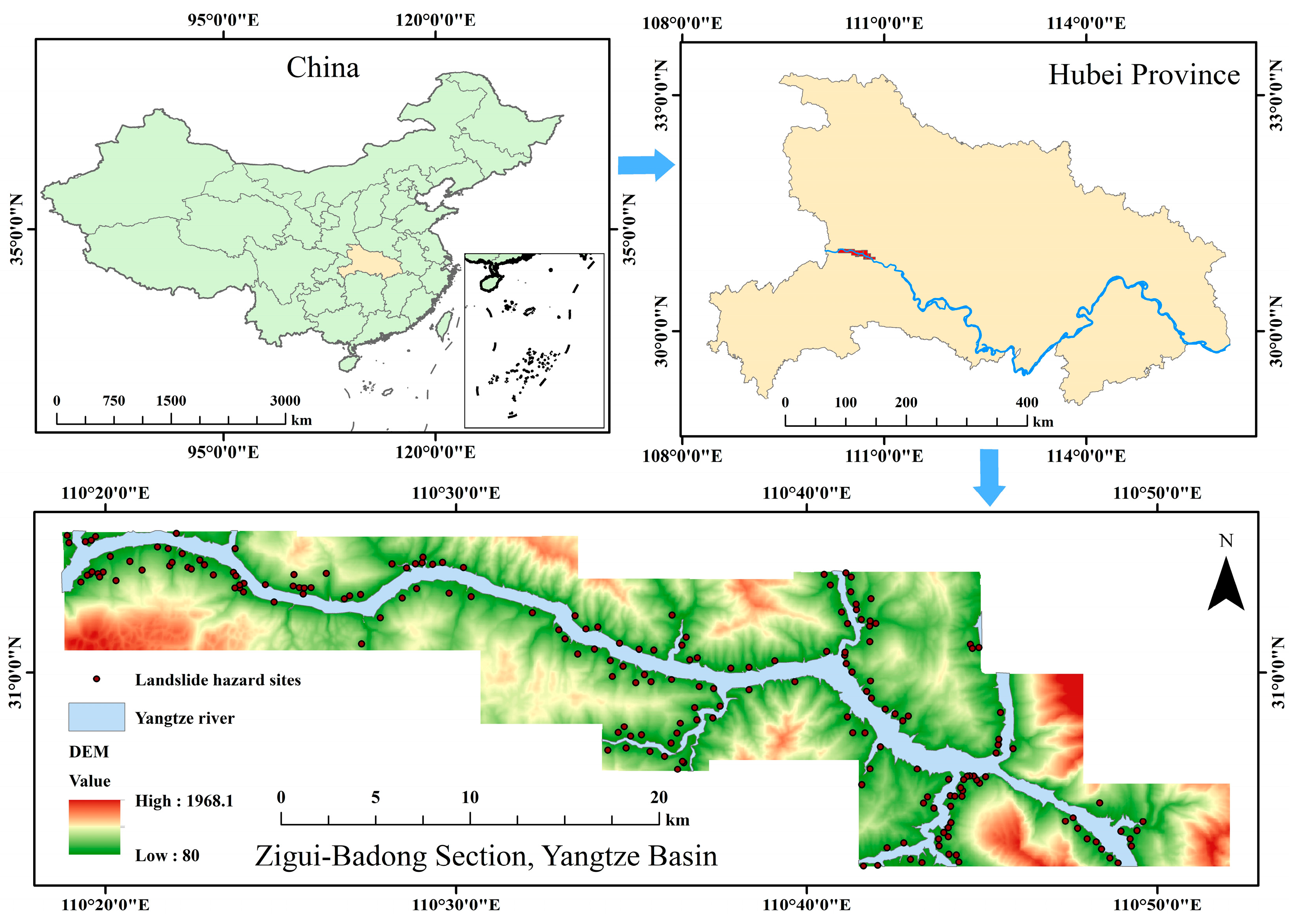
Figure 1. Study area of the Zigui to Badong section of the Yangtze River Basin.
Applsci 16 00430 g001
Figure 2. The study area in Ya'an City, Sichuan Province.
Applsci 16 00430 g002
Figure 3. Flowchart of the proposed MFP_Stacking process.
Applsci 16 00430 g003
Figure 4. Multidimensional vector production.
Applsci 16 00430 g004
Figure 5. Self-training and multi-network collaboration.
Applsci 16 00430 g005
Figure 6. A Stacking model framework based on multidimensional feature collaboration.
Applsci 16 00430 g006
Figure 7. Spearman correlation coefficients of the LCFs.
Applsci 16 00430 g007
Figure 8. Gini indices of the LCFs.
Applsci 16 00430 g008
Figure 9. Map of 9 modeling results for the section from Zigui to Badong. (a) RF (b) TabNet (c) LeNet (d) ViT (e) CLNet (f) 1D_Stacking (g) 2D_Stacking (h) MF_Stacking (i) MFP_Stacking.
Applsci 16 00430 g009aApplsci 16 00430 g009b
Figure 10. Map of 9 modeling results for Ya’an. (a) RF (b) TabNet (c) LeNet (d) ViT (e) CLNet (f) 1D_Stacking (g) 2D_Stacking (h) MF_Stacking (i) MFP_Stacking.
Applsci 16 00430 g010aApplsci 16 00430 g010b
Figure 11. ROC curves of all models.
Applsci 16 00430 g011
Figure 12. Landslide susceptibility zoning map of the Zigui–Badong section based on the MFP_Stacking model: (a) LSM generated by MFP_Stacking; (b,d) areas of landslides outside the training labels; (c,e) corresponding susceptibility maps.
Applsci 16 00430 g012
Figure 13. Landslide susceptibility zoning map of Ya’an City based on the MFP_Stacking model: (a) LSM generated by MFP_Stacking; (b,d,f) areas of landslides outside the training labels; (c,e,g) corresponding susceptibility maps.
Applsci 16 00430 g013
Table 1. Source of sample.
TypeData SourceStudy AreaNumber
positive sampleResource and Environment Science Data CenterZigui–Badong section197
Ya’an City737
negative sampleInformation Value MethodZigui–Badong section197
Ya’an City737
Table 2. Data sources for LCFs.
DataZigui–Badong SectionYa’an City
Data TypeLCFsData SourceResolutionData SourceResolution
Topography & GeomorphologyElevationASTER GDEM Version 230 mALOS 12.5 m Digital
Elevation Model
Downsampled from 12.5 m to 30 m
Slope
Aspect
Plan Curvature
Profile Curvature
Geological SettingsDistance to FaultGeological map from the Hubei Geological Bureau1:50,000Geological map from the China Geological Survey1:2,500,000
Lithology
HydrometeorologyRainfallNational Meteorological Information Center
(2001–2010)
-National Meteorological Information Center
(2013–2020)
-
Distance to DrainageASTER GDEM Version 2-2 m Google imagery-
Land CoverLand UseLandsat 5 TM images (2010)30 mESA land cover data10 m
NDVISentinel-2 satellite data (2020)10 m
Table 3. Summary of single classifiers: Mechanisms, Advantages and Limitations, Applicable Scenarios, and Roles in Stacking.
ClassifierMechanismAdvantagesLimitationsApplicable
Scenarios
Specific Role in Stacking
RFEnsembles multiple decision trees and integrates predictions via a voting mechanismRobust to overfitting, handles high-dimensional features, insensitive to outliersLimited in capturing complex nonlinear relationships, less interpretableStructured data classification, feature importance analysisProcesses 1D vectors, provides robust baseline predictions, enhances ensemble diversity and generalization
TabNetUses attention to select features, leveraging sequence to capture interactions.Outperforms traditional DL on tabular dataHigh computational complexity, hyperparameter tuning challengingTabular data modeling requiring feature selectionProcesses 1D vectors, captures complex interactions overlooked by RF, contributes diverse predictions
LeNetExtracts local spatial features through convolutional layers and reduces dimensionality via poolingStrong local feature extraction, efficient via parameter sharing, translation invariantLimited receptive field, cannot capture global dependenciesImage classification, local pattern recognitionProcesses 3D vectors, learns local environmental influence on landslides, provides spatially local perspective
ViTSplits input into patches, models global dependencies via self-attentionGlobal receptive field, captures long-range dependenciesHigh data requirement, computationally expensiveTasks needing global context understandingProcesses 3D vectors, models global spatial patterns, complements LeNet’s local focus
Table 4. Hyperparameter search space for all models.
ModelHyperparameter and Search Space
RFn_estimators: {50, 60, 70, …, 150}; max_depth: {6, 8, 10, 12}; max_features: {“sqrt”, “auto”}
TabNetn_d, n_a: {8, 9, 10, …, 16}; n_steps: {3, 4, 5}; Gamma: {1, 1.1, 1.2}; lr: {0.0001, 0.0005, …, 0.01}
LeNetlr: ibid.; Batch size: {32, 64, 128}; Epochs: {300, 400, 500}; Patience: {10, 20, …, 60, Early stopping}
ViTlr: ibid.; patch_size: {3}; Embedding dimension (ED): {64, 128, 256}; MLP ratio: {2, 4};
batch size: {32, 64, 128}; Epochs: {100, 200, 300, 400}; Patience: {10, 20, 30, 40, Early stopping}
CLNetlr, patch_size, ED, MLP ratio, batch size, Epochs, Patience: ibid.; cnn_outdim: {32, 64, 128, 256}
StackingMeta-model type: {weighted linear regression}; Cross-validation folds: {3, 4, 5}
Table 5. Model hyperparameter settings.
ModelZigui–Badong SectionYa’an City
ParametersParameters
RFn_estimators = 100; max_depth = 8;
max_features = ‘auto’
n_estimators = 50; max_depth = 8;
max_features = ‘auto’
TabNetn_d = 14; n_a = 14; n_steps = 3; gamma = 1.1; lr = 0.001n_d = 13; n_a = 13; n_steps = 3; gamma = 1.1; lr = 0.001
LeNetbatch_size = 64; epochs = 400; patience = 50; lr = 0.001batch_size = 64; epochs = 400; patience = 50; lr = 0.005
ViTpatch_size = 3; ED = 128; patience = 20; lr = 0.0001; mlp_ratio = 4; batch size = 64; epochs = 200patch_size = 3; ED = 128; patience = 10; lr = 0.0001; mlp_ratio = 4; batch size = 64; epochs = 100
CLNetpatch_siz, ED, patience, mlp_ratio, batch size, epochs: ibid.; lr = 0.001; cnn_outdim = 64patch_siz, ED, patience, mlp_ratio, batch size, epochs: ibid; lr = 0.001; cnn_outdim = 64
1D_StackingSingle classifiers: SVM, TabNet, RF; Meta-model: weighted linear regression; cross-validation: 5-foldSingle classifiers: GBDT, TabNet, RF; Meta-model: weighted linear regression; cross-validation: 3-fold
2D_StackingSingle classifiers: CNN, LeNet, ViT; Meta-model: ibid.; cross-validation: ibid.Single classifiers: LeNet, ViT; Meta-model: ibid.; cross-validation: ibid.
MF_StackingSingle classifiers: RF, TabNet, LeNet, ViT, Meta-model: ibid.; cross-validation: ibid.Single classifiers: RF, TabNet, LeNet, ViT, Meta-model: ibid.; cross-validation: ibid.
MFP_StackingSingle classifiers: ibid., Meta-model: ibid.; cross-validation: ibid.; Number of pseudo-labels: 200 × 4; Segmented selection of pseudo-labels: 1–0.8:0.8–0.6:0.6–0.4 = 6:3:1Single classifiers: ibid., Meta-model: ibid.; cross-validation: ibid. Number of pseudo-labels: 280 × 4; Segmented selection of pseudo-labels: 1–0.8:0.8–0.6:0.6–0.4 = 6:3:1
Table 6. Statistical table of landslide susceptibility evaluation of each model.
ModelSusceptible PartitionZigui–Badong SectionYa’an City
PCPLLDPCPLLD
TabNetVery low0.31400.00000.00000.41770.01590.0380
Low0.21880.01520.06950.15590.02380.1527
Moderate0.15480.04060.26230.10900.05290.4853
High0.14600.18781.28630.10710.14551.3581
Very high0.16650.75634.54230.21020.76193.6248
RFVery low0.47410.00000.00000.44120.01720.0390
Low0.19000.01520.08010.15230.02910.1911
Moderate0.08630.01520.17650.13330.08600.6450
High0.09120.07610.83460.11030.18121.6422
Very high0.15840.89345.63950.16280.68654.2159
LeNetVery low0.48630.00000.00000.24410.00130.0050
Low0.12820.02030.15840.23320.02120.0907
Moderate0.09310.03050.32710.18420.04630.2514
High0.10810.13201.22070.13900.15081.0850
Very high0.18430.81734.43440.19960.78043.9107
VITVery low0.63260.01010.01600.51720.02120.0409
Low0.06240.01010.16270.12850.03440.2677
Moderate0.05280.03050.57720.08020.05030.6271
High0.07310.08631.18100.07950.09791.2318
Very high0.17920.86294.81490.19470.79634.0887
CLNetVery low0.65940.01520.02310.48600.01450.0299
Low0.05680.02030.35770.16530.03040.1840
Moderate0.04900.04060.82940.06150.03700.6018
High0.06520.09141.40020.05210.05561.0653
Very high0.16960.83254.90820.23490.86243.6709
1D_StackingVery low0.45340.00000.00000.56150.02910.0518
Low0.18040.01520.08440.07680.01590.2066
Moderate0.09920.02540.25590.06580.02510.3818
High0.09600.13711.42760.07480.09921.3260
Very high0.17090.82234.81090.22100.83073.7583
2D_StackingVery low0.56330.00510.00900.49740.00930.0186
Low0.12120.01520.12560.13830.02780.2009
Moderate0.06630.03550.53560.07520.04100.5453
High0.07640.12181.59360.07480.08331.1146
Very high0.17270.82234.76180.21430.83863.9129
MF_StackingVery low0.54840.00510.00930.48840.00790.0162
Low0.13040.01010.07780.13670.02780.2032
Moderate0.07130.02540.35610.08230.04100.4982
High0.08130.11671.43520.08300.08331.0034
Very high0.16850.84264.99900.20950.83994.0093
MFP_StackingVery low0.51900.00510.00980.53180.00930.0174
Low0.14710.00510.03450.11130.02510.2259
Moderate0.08180.01520.18630.05680.03310.5823
High0.09130.10151.11140.08660.11381.3140
Very high0.16080.87315.43100.21350.81883.8348
Table 7. Evaluation metrics of all models.
Research AreaModelPerformance
OaKappaPrecisionRecallF1MCCAuc
Zigui–Badong sectionTabNet0.84750.69490.83610.86440.85000.69530.8805
RF0.85590.71240.80280.91380.86180.71740.9114
LeNet0.81360.62890.73680.96550.83580.66010.9112
ViT0.83050.66190.77940.91380.84130.67160.9017
CLNet0.84750.69540.81250.89660.85250.69000.9187
1D_Sk0.85600.71250.80600.93100.86400.72090.9239
2D_Sk0.84750.69550.80300.91380.85480.70200.9129
MF_Sk0.87280.74630.82090.94830.88000.75510.9282
MFP_Sk0.88130.76320.83330.94830.88710.77030.9353
Ya’an CityTabNet0.91270.82540.91270.91260.91280.82540.9692
RF0.91610.83220.91890.91270.91580.83220.9699
LeNet0.88760.77520.84480.94960.89410.78120.9542
ViT0.90530.81060.89610.91680.90640.81080.9639
CLNet0.92100.84190.91870.92370.92120.84190.9703
1D_Sk0.92090.84170.90650.93860.92230.84230.9773
2D_Sk0.92170.84330.91430.93050.92230.84350.9742
MF_Sk0.92850.85690.91880.94010.92930.85720.9814
MFP_Sk0.93800.87600.92810.94960.93870.87630.9855
Table 8. The parameter count and computational efficiency of each base model.
Research AreaModelParameter CountTraining Time per Epoch (s/epoch)Total Training Time (s)Inference Time (ms/Sample)
Zigui–Badong sectionRFNoNo0.7711.9600
TabNet4.24 K0.4094520.6480
LeNet0.245 M0.1252470.2241
ViT2.21 M1.5833571.8513
CLNet2.32 M2.0976861.7733
Ya’an CityRFNoNo0.5540.5054
TabNet5.37 K0.95001330.5165
LeNet0.245 M0.4600140 s0.1988
ViT2.21 M5.17851451.2743
CLNet2.32 M7.48152022.3556
Table 9. AUC variation with different percentages of the training set.
Research AreaModelPercentage of the Training Set
102030405060708090
Zigui–Badong sectionTabNet0.30710.34270.35760.85290.85900.87540.88050.86850.8476
RF0.86890.87740.88420.89810.90520.90090.91140.89550.8864
LeNet0.88470.90050.90680.91370.91820.91430.91120.90950.9132
ViT0.76120.85440.90020.90100.90100.91050.90170.90490.9209
CLNet0.84510.87440.89530.89850.91140.91910.91870.91370.9200
1D_Sk0.88090.88680.89760.91660.91800.92090.92390.91720.9114
3D_Sk0.88740.89910.91310.91390.91880.91500.91300.91000.9250
MF_Sk0.90190.91270.91880.92060.92860.92760.92820.92880.9305
Ya’an CityTabNet0.87240.92920.94420.95550.94720.96140.96920.97110.9750
RF0.93610.95010.96030.96860.97030.97050.96990.97260.9739
LeNet0.92940.93590.94230.94840.95220.95440.95420.95180.9493
ViT0.92180.92350.93120.93990.95010.96060.96390.94450.9432
CLNet0.92510.94090.94910.95510.96530.97040.97030.97210.9740
1D_Sk0.94050.95390.96090.96630.97160.97400.97730.97270.9754
3D_Sk0.93060.93700.94740.95440.96580.96570.97420.97400.9701
MF_Sk0.94910.95860.96370.96790.97600.97770.98140.97730.9788
Table 10. AUC values obtained under different segmentation ratios and quantities during the pseudo-label selection process.
Research AreaRatios; Pseudo-Label Selection Strategy; Final NumberAUCW m e a n _ p
Zigui–Badong section1–0.8:0.8–0.6:0.6–0.4 = 1:0:0; 200 × 4; 5500.93830.870.0619
1–0.8:0.8–0.6:0.6–0.4 = 7:3:0; 200 × 4; 5500.92230.820.0653
1–0.8:0.8–0.6:0.6–0.4 = 6:4:0; 200 × 4; 5500.92160.810.0983
1–0.8:0.8–0.6:0.6–0.4 = 5:5:0; 200 × 4; 5500.91840.780.0963
1–0.8:0.8–0.6:0.6–0.4 = 6:3:1; 200 × 4; 5500.93530.780.0989
1–0.8:0.8–0.6:0.6–0.4 = 6:2:2; 200 × 4; 5500.91060.750.0733
1–0.8:0.8–0.6:0.6–0.4 = 6:3:1; 100 × 4; 2700.93490.830.1312
1–0.8:0.8–0.6:0.6–0.4 = 6:3:1; 300 × 4; 8500.91330.760.0747
1–0.8:0.8–0.6:0.6–0.4 = 6:3:1; 400 × 4; 10900.89340.720.0558
Ya’an City1–0.8:0.8–0.6:0.6–0.4 = 1:0:0; 280 × 4; 7600.98920.900.1531
1–0.8:0.8–0.6:0.6–0.4 = 7:3:0; 280 × 4; 7600.97510.870.1689
1–0.8:0.8–0.6:0.6–0.4 = 6:4:0; 280 × 4; 7600.97340.800.1626
1–0.8:0.8–0.6:0.6–0.4 = 5:5:0; 280 × 4; 7600.97100.840.1531
1–0.8:0.8–0.6:0.6–0.4 = 6:3:1; 280 × 4; 7600.98550.810.1760
1–0.8:0.8–0.6:0.6–0.4 = 6:2:2; 280 × 4; 7600.96940.790.1536
1–0.8:0.8–0.6:0.6–0.4 = 6:3:1; 140 × 4; 3800.98130.810.2144
1–0.8:0.8–0.6:0.6–0.4 = 6:3:1; 420 × 4; 11200.97260.780.1262
1–0.8:0.8–0.6:0.6–0.4 = 6:3:1; 560 × 4; 15000.96090.770.0851
Disclaimer/Publisher’s Note: The statements, opinions and data contained in all publications are solely those of the individual author(s) and contributor(s) and not of MDPI and/or the editor(s). MDPI and/or the editor(s) disclaim responsibility for any injury to people or property resulting from any ideas, methods, instructions or products referred to in the content.