Article

LIDAR Observation and Numerical Simulation of Building-Induced Airflow Disturbances and Their Potential Impact on Aircraft Operation at an Operating Airport

1
Hong Kong Observatory, 134A Nathan Road, Kowloon, Hong Kong, China
2
Department of Civil and Environmental Engineering, The Hong Kong Polytechnic University, Hong Kong, China
*
Author to whom correspondence should be addressed.
Appl. Sci. 2026, 16(1), 404; https://doi.org/10.3390/app16010404 (registering DOI)
Submission received: 3 November 2025 / Revised: 29 December 2025 / Accepted: 29 December 2025 / Published: 30 December 2025

Abstract

Observations of building-induced airflow disturbances arising from the new terminal building at the Hong Kong International Airport (HKIA) are documented in this paper. Two case studies are conducted: one involving turbulent flow downstream of the building and another involving a coherent “building-induced wave”. To capture these phenomena under realistic atmospheric forcing, we employ a coupled mesoscale–computational fluid dynamics modelling system. This approach integrates mesoscale boundary-layer conditions with building-resolving simulations for real airport disturbance analysis. The main features of the actual observation are largely captured by the simulations. As such, the simulated data are studied to find out the reason for the difference in the airflow behavior. The difference could be related to the stability of the “background” atmospheric boundary layer. This stability is influenced by a number of complicated factors, including the background mesoscale atmospheric stability, Foehn effect of the terrain, and solar heating of the sea/land surface. The study further discusses potential implications for runway operations using aviation-relevant indicators, including the 7-knot criterion and turbulence intensity.
Keywords:
LIDAR; aviation; CFD

1. Introduction

Buildings and other large obstacles can substantially modify the atmospheric boundary-layer flow by forcing deceleration, flow separation, and strong shear layers around edges. The resulting disturbance field typically includes a combination of recirculation zones, enhanced turbulence kinetic energy, intermittent vortex shedding, and a downstream recovery region. The length and structure of these disturbance fields depend on obstacle geometry (height, width, aspect ratio, and porosity), surface roughness, and the characteristics of the incoming boundary layer [1,2,3,4]. A key control is the thermodynamic stability of the atmospheric boundary layer [5]. In stable stratification, vertical displacements are suppressed, and shear layers and obstacle-forced perturbations can remain more organized and persist farther downstream. In neutral or weakly stratified conditions, stronger mixing tends to promote a more rapidly dispersing, turbulence-dominated response. These processes are central to urban flow and dispersion, pedestrian wind comfort, and wind loading. They are routinely studied using wind-tunnel experiments and computational fluid dynamics (CFD), including large-eddy simulation (LES) [6,7,8,9,10,11].
In the airport environment, the same building–boundary-layer interactions can become an operational hazard because approach and departure occur at low altitude. At these heights, aircraft are sensitive to rapid wind changes, localized shear, and turbulence. As airports expand, large terminals, hangars, and ancillary structures may be constructed close to runway corridors due to land constraints. This increases the probability that obstacle-induced disturbed flow intersects the flight path. The operational consequence is not merely a reduction of mean wind speed. Rather, transient fluctuations in headwind/crosswind components and enhanced turbulence can elevate the risk of low-level wind shear events and degraded handling qualities during take-off and landing.
Recognizing these risks, airport operators and meteorological services have developed assessment approaches and practical wind/obstacle criteria [12,13]. In parallel, observational capabilities have advanced: Doppler LIDAR systems are now widely deployed to diagnose near-runway wind disturbances as they provide spatially resolved wind measurements and can capture evolving disturbance patterns in real time [13,14,15,16]. On the modelling side, high-resolution CFD/LES has increasingly been used to interpret observations, explore sensitivity to wind direction and stability, and provide scenario-based guidance for infrastructure planning [17,18,19]. Nevertheless, its computational cost still limits operational, real-time deployment.
This issue is particularly relevant at Hong Kong International Airport (HKIA), which is built on a reclaimed island with dense infrastructure. For the sustainable development of the airport, apart from facilities supporting air navigation, there are many other buildings (e.g., terminal building, hangar, and shopping plaza) on this island. Due to the limited space on the island, some buildings may be built at locations rather close to the runways of HKIA. Previous numerical simulations (e.g., ref. [19]) found that certain buildings may cause airflow disturbances over the runways, especially in northerly wind situations associated with tropical cyclones.
With the opening of the third runway (new north runway) of HKIA in 2024, a new terminal (location in Figure 1) has been constructed close to it. This terminal has a height of about 40 m above ground, and its height to distance ratio with respect to the center runway (runway corridor 25CA/07CD, Figure 1) is about 1:20. It is smaller than 1:35 for the building’s effect on the low-level wind as found in the studies for Schiphol airport of the Netherlands [12]. Therefore, this new terminal may cause airflow disturbances near the eastern end of the center runway under northerly wind conditions. In order to monitor the airflow disturbances, a short-range LIDAR (SRL) has been set up at the location called X25 (Figure 1). The SRL scans in the vertical range-height indicator (RHI) mode perpendicular to the eastern end of the center runway. Against this background, the present study combines SRL observations with high resolution CFD simulations driven by a mesoscale model to assess the capability of the modelling system to reproduce the observed signature. This study also examines how the boundary-layer stability modulates the building-induced disturbance. More broadly, improving understanding of these effects supports global operational safety. It informs airport layout and expansion planning and strengthens wind-hazard forecasting and alerting for approach and departure corridors.

2. Meteorological Instrumentation

In the present study, Doppler velocity images of two LIDARs are used, namely, a long-range LIDAR (LRL, Figure 1b) just to the south of the north runway (location marked by HKG3S in Figure 1a) and the SRL (Figure 1c) at the location X25. Both use laser beams with a central wavelength of about 1.5 micron. The LRL is mainly used to provide glide-path scan data for windshear detection. Additionally, the LRL also performs plan position indicator (PPI) scans. The scanning data are used to calculate a map of turbulence intensity, namely, eddy dissipation rate (EDR) over the airport region (based on the structure function approach according to the method in [13]). The LRL has a spatial coverage of about 15 km and a spatial resolution of about 100 m. PPI scans are updated every 2 to 4 min, depending on the scan strategy.
SRLs are used at HKIA mainly for the monitoring of aircraft wake and building-induced airflow disturbances. For these purposes, the SRL mostly performs RHI scans. It has a spatial coverage up to 3 km with a spatial resolution of around 10 m. Data are updated every 1 min or so. In addition, some SRLs are configured to perform PPI scans and Doppler swinging for providing vertical wind profiles every 2 min or so.

3. Setup of Numerical Models

The setup of the mesoscale meteorological model, namely, RAMS, was similar to that in [20]. A brief summary of the setup is given here. The boundary conditions for RAMS were provided by the hourly reanalysis of the European Centre for Medium-Range Weather Forecasts (ECMWF Reanalysis v5 or ERA5) with a spatial resolution of 25 km. Five nests were implemented in RAMS, with horizontal resolutions of 25 km, 5 km, 1 km, 200 m, and 40 m. The nested configuration is designed to progressively downscale from synoptic-to-mesoscale to the airport/building scale while maintaining dynamically consistent boundary-layer structures. Their domains are shown in Figure 2a,b. The choice of turbulence parameterization scheme is critical for the successful simulation of the required features. Here, the first two nests used the Smagorinsky scheme [21] while the other three nests used the Deardorff scheme [22]. The Smagorinsky closure was used in the two outer nests. At these resolutions, boundary-layer turbulence is entirely sub-grid and a simple eddy-viscosity formulation is sufficient. The inner three nests used the Deardorff scheme, as turbulence becomes partly resolved and a prognostic turbulent kinetic energy scheme better captures shear- and stability-dependent mixing. The first model level is around 30 m, and vertical levels have a stretching ratio of 1.08. The highest model level has a height of around 1200 m.
Although the innermost RAMS nest reached 40 m resolution, it still cannot explicitly resolve flow separation and wake turbulence induced by individual buildings. Therefore, RAMS was coupled to the CFD model PALM [23,24,25] to simulate airflow disturbances arising from the buildings. The building configuration is shown in Figure 1a. The model domain for PALM is shown in Figure 2c.
The PALM model solves nonhydrostatic, incompressible Navier–Stokes equations under the Boussinesq approximation, using a 1.5-order turbulence closure scheme [22]. The Boussinesq approximation was adopted because the simulations target a relatively shallow domain in which fractional density variations are small. Therefore, density can be treated as constant except in the buoyancy term. The Boussinesq approximation preserves the effects of stratification on wake and wave development while filtering acoustic modes and reducing computational cost. PALM has been extensively evaluated against laboratory experiments, field observations, and established benchmark cases for atmospheric boundary-layer flows and urban-resolving applications [26,27,28].
Momentum advection was solved through a fifth-order upwind scheme [29]. A third-order Runge–Kutta method [30] was applied for time integration. The horizontal resolution was 6 m. For the vertical grid, the initial resolution was 4 m, with a stretching factor of 1.08 applied from 50 m upward, and the maximum value is capped at 12 m. The domain top was about 1300 m.
The offline coupling between RAMS and PALM was implemented using PALM’s dynamic driver input file. RAMS output was post-processed to create a dynamic input file that provided the initial condition and the time-varying lateral and top boundary conditions (Dirichlet boundary conditions) for PALM. The dynamic input file contained the meteorological variables required by PALM, including the three wind components, potential temperature, and water–vapor mixing ratio. The dynamic driver was updated every 10 min, following the RAMS output frequency. PALM provides Python (https://gitlab.palm-model.org/releases/palm_model_system/-/tree/master/packages/dynamic_driver/wrf_interface, accessed on 3 November 2025) scripts to extract, interpolate, and write these fields in the dynamic-driver format (originally designed for WRF output). In this study, these scripts were modified so that the same procedure could be applied to RAMS output, i.e., to read the RAMS variables and generate the required PALM dynamic input file. No turbulent fluctuations were prescribed from RAMS at the inflow boundaries; instead, a synthetic turbulence generator was applied to generate a turbulent inflow condition [31,32]. Details of the coupling procedure are given in [20].

3.1. Case Study 1: 15 January 2025

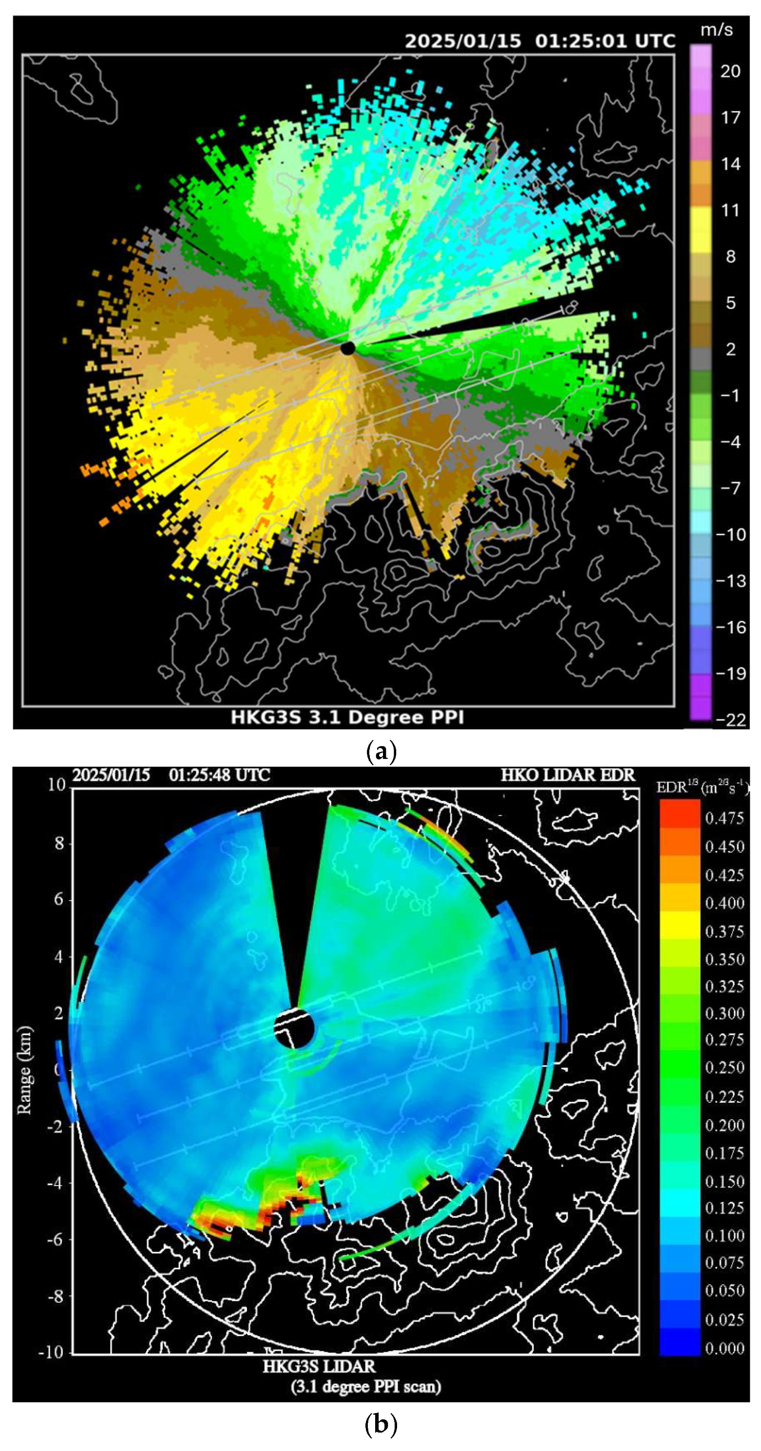
The northeast monsoon prevailed over southern China on the morning of Case Study 1. From the LRL PPI scan, northeasterly winds of around 11 m/s prevailed over the airport region (Figure 3a). In this paper, the radial velocity (and the derived along-beam component) follows the standard sign convention: positive values indicate flow away from the LIDAR, whereas negative values indicate flow toward the LIDAR. Due to the disruption by the terrain to the northeast of HKIA, the airflow appeared to be rather disturbed to the northeast of the LRL. The EDR is also higher over there (Figure 3b), reaching a moderate turbulence level (EDR of around 0.3 m2/3 s−1). At the same time, moderate turbulence was also observed just to the east of the LRL, when winds were blowing over the new terminal (Figure 3b).
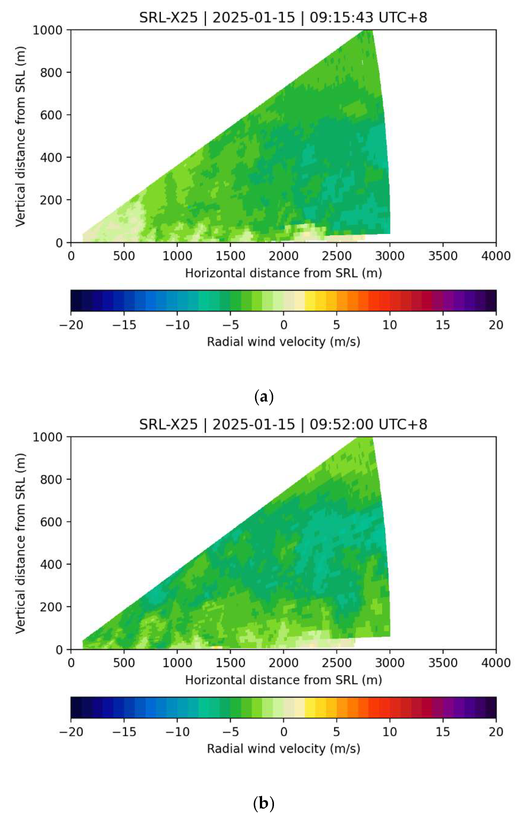
The RHI scan of the SRL is shown in Figure 4 (location of the scan shown in Figure 1a) for two different times. In the RHI plot, the x-axis represents the horizontal distance along the RHI beam from the SRL X25 site; positive values correspond to increasing distance toward the north (i.e., along the scan direction). At around 2500 m from SRL, there is blockage of the laser beam due to the new terminal building. The 25CA/07CD runway is located about 1800 m downstream of the SRL. Winds are blowing from right to left in the figure. It can be seen that, downstream of the new terminal building, there are various areas with weak and even reverse flow, extending vertically to about the height of this building. Aloft of the new terminal building, there was an area of stronger northerly winds, with wind speeds reaching about 9 m/s. The stronger northerly winds remained above the building height.
The results of the PALM simulation were compared with the observations from the LRL and SRL to confirm their validity. Figure 5a compared the crosswind distribution. The simulated and SRL-observed crosswind distributions at the intersection of the SRL RHI plane and the 25CA/07CD runway were comparable, with both peaking around −4 m s−1. However, the distribution was wider for the simulation, with more crosswinds of higher speed as compared with the actual SRL observations. This was related to the descent of a northerly jet (of around 9 m/s) closer to the surface in the simulation, whereas in the actual SRL observations, the winds were mostly disturbed by the new terminal building with a lower wind speed. The headwind profile along 25CA/07RD was captured by another LRL, HKG2 (location in Figure 1). The data were compared with the simulation result in Figure 5b. The two datasets were generally comparable. The RMSE and bias were 0.71 and −0.081 m/s, respectively.
Based on experience at the Amsterdam Schiphol Airport, a crosswind-variation threshold of 7 knots was introduced as an operationally relevant criterion. It was subsequently adopted by the ICAO Aerodrome Meteorological Observation and Forecast Study Group (AMOFSG) in Doc 8896 (Manual of Aeronautical Meteorological Practice) to assist states in the planning of buildings at aerodromes. Accordingly, we applied the “7-knot criterion” (7 kt ≈ 3.6 m s−1) in this study to assess potential operational impact as studied in [33], though the background crosswind speed is not exactly 25 knots. The simulation and measured time series of crosswind speed at a height of 50 m at the point of intersection between SRL RHI plane and 25CA/07RD was shown in Figure 5c. The two datasets were generally comparable, and the RMSE and bias were 1.65 m/s and −0.43 m/s, respectively. Furthermore, the maximum crosswind changes were in the order of around 3 m/s, which was close to the 7-knot criterion.
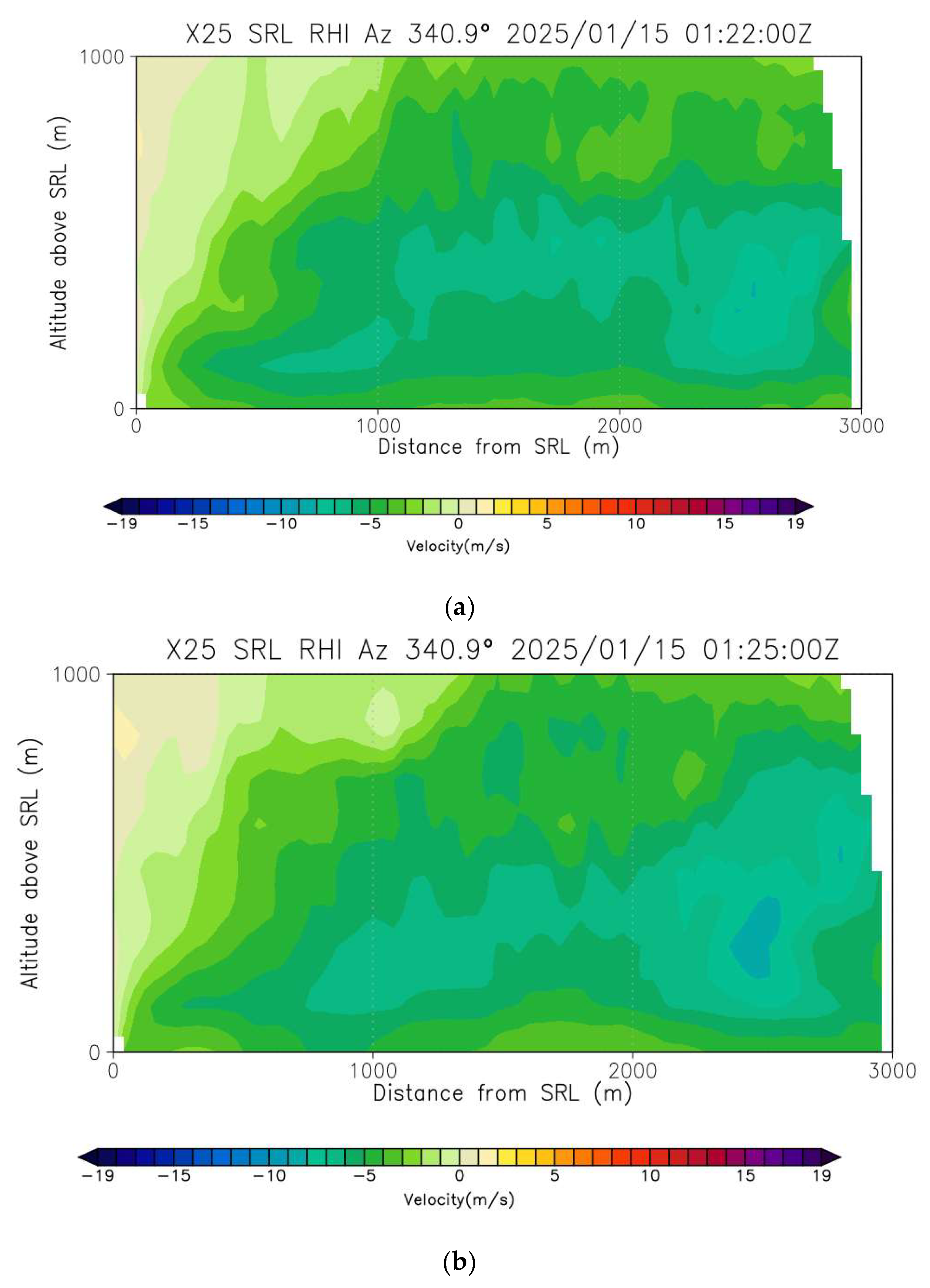
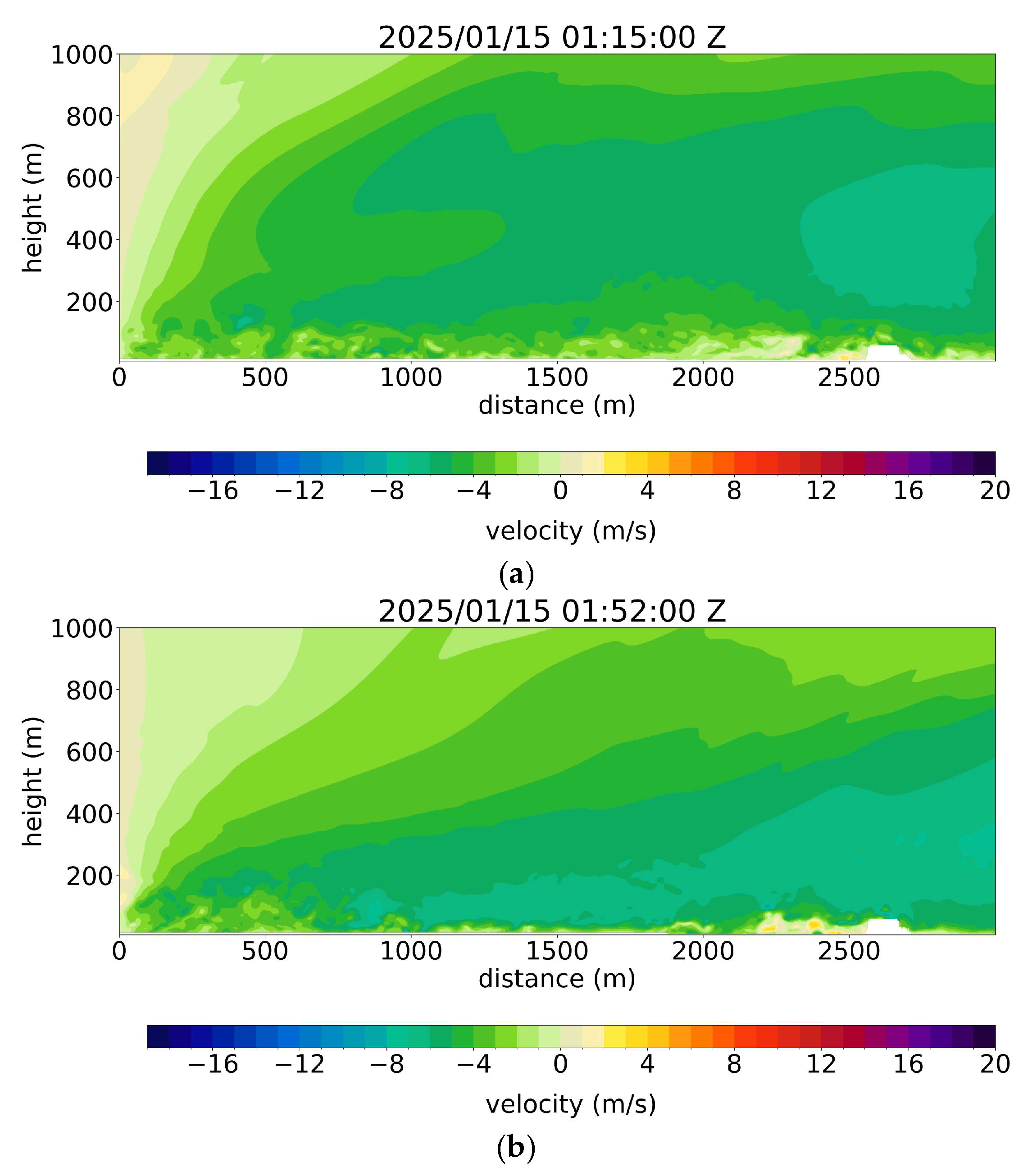
The simulation results were examined further, in order to check that the observed and the simulated airflow disturbances near the ground are indeed due to disruption by the new terminal building. Firstly, the background meteorological field as simulated by RAMS was shown in Figure 6 for a couple of time instances. The simulated RHI scans indicated that terrain-induced flow alone did not produce disturbances such as reverse flow. The signature of the disturbance was clear in the PALM simulation with the inclusion of the new terminal building, with samples shown in Figure 7. Compared with the actual observation in Figure 4a, the vertical extent of the disturbance was slightly lower in the simulation in Figure 7a. Aloft of the new terminal building, there was an area of enhanced northerly flow in the simulation, again consistent with the actual observation in Figure 4a. This area of enhanced northerly flow descended at a later time, as shown in Figure 7b, but such a descent was absent in the observation (Figure 4b). This explains the discrepancy in crosswind distribution as shown in Figure 5a.
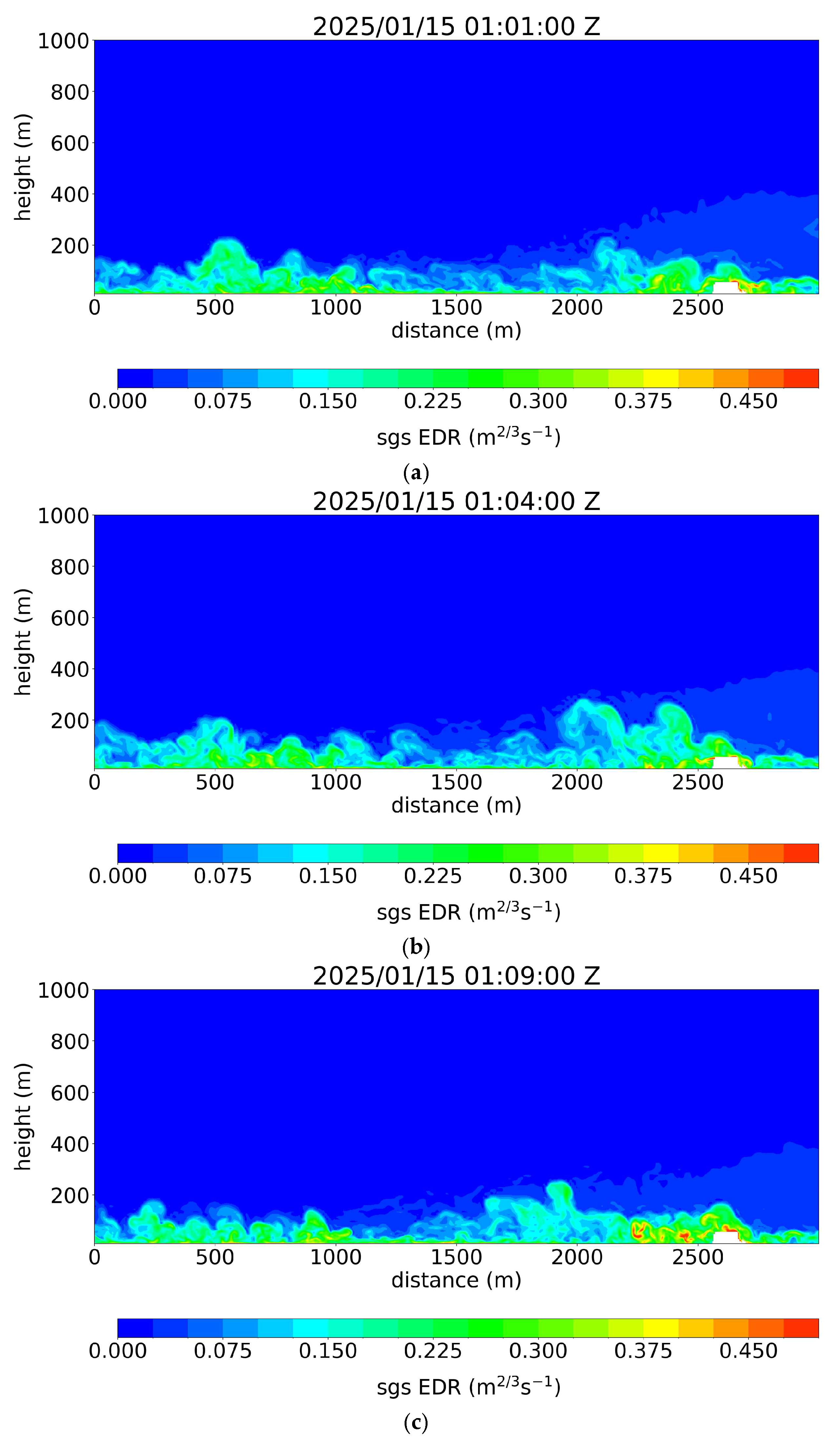
To further study the impact of the new terminal building on the airflow, the (sub-grid-scale) EDR time sequence was shown in Figure 8. At first, the more turbulent flow (higher EDR, reaching moderate intensity) was found around the building (Figure 8a). It then propagated downstream (Figure 8b) and crossed the runway location (around 1800 m downstream of the SRL, Figure 8c). So, the building may have had an impact on the aircraft departing from 07CD. The higher EDR above the new terminal building in the simulation (Figure 8) was consistent with the actual EDR map (Figure 3b). It should be noted that the LIDAR EDR is derived from the second-order structure function of measured radial velocities and represents an effective dissipation estimate over the instrument’s sampling volume, whereas the model EDR shown here is diagnosed directly from the turbulence kinetic energy equation. These differences in spatial–temporal averaging and the intermittent nature of turbulence preclude a direct quantitative one-to-one comparison. A more comprehensive EDR intercomparison will be pursued in future work.
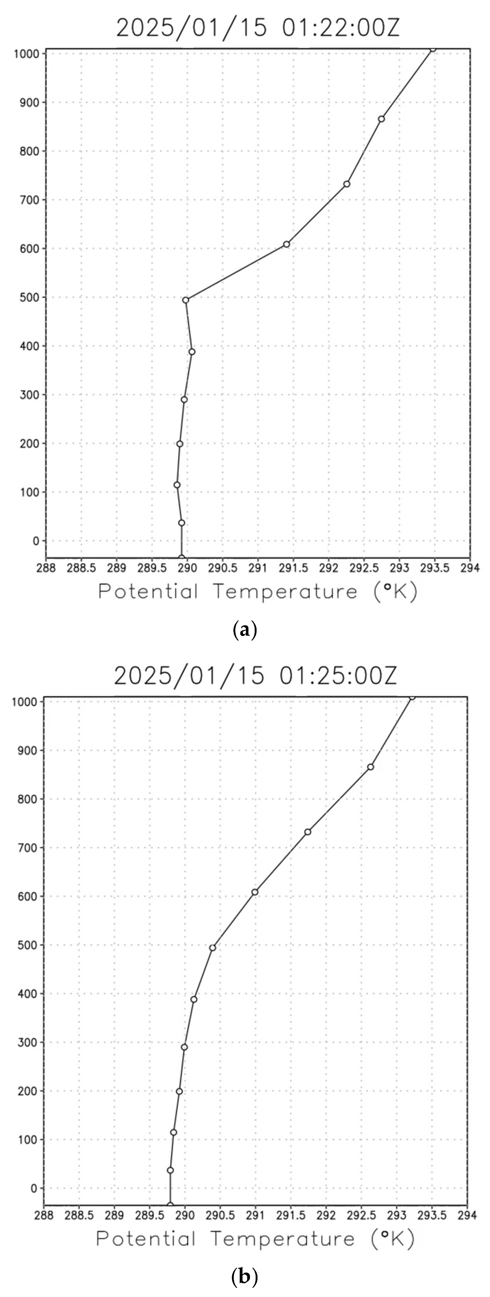
In this case, only turbulent flow was found downstream of the building. No coherent structure, such as a wave, could be found in the observation and simulation. The potential temperature profile at a point upstream of the new terminal building (location in Figure 1a) was shown in Figure 9 for two time instances. It was found that, below 400 to 500 m or so above sea level, the atmospheric boundary layer is near neutral, as indicated by small values of the Brunt–Väisälä frequency squared, N 2 (e.g., N 2 = 9.50 × 10 6   s 2 at 50 m and N 2 = 1.31 × 10 6   s 2 at 350 m at 01:22 UTC on 15 January 2025). Such weak (near-neutral to weakly stable) stratification was consistent with the absence of a persistent, coherent wave-like response in this case.

3.2. Case Study 2: 26 January 2025

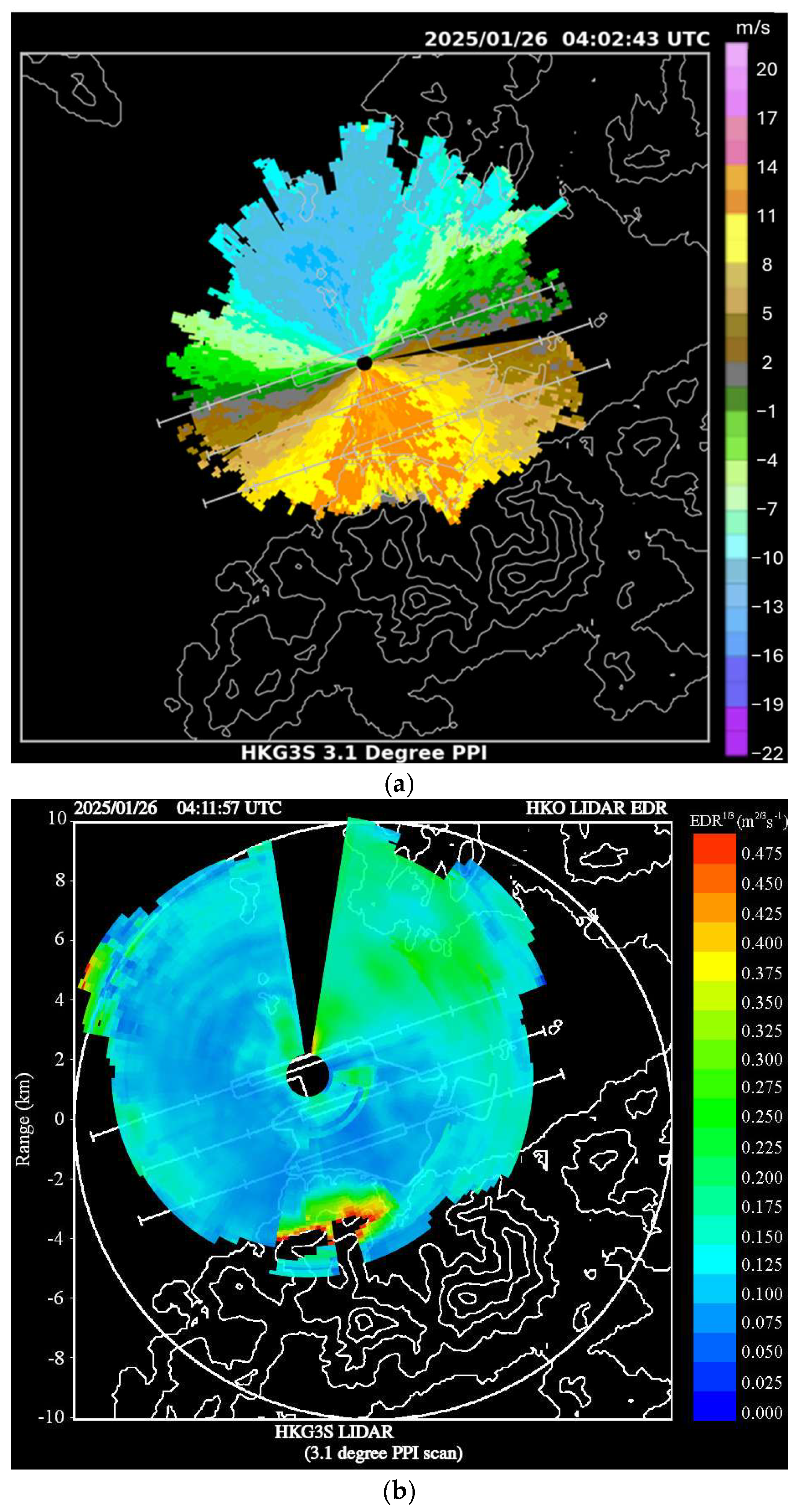
For the second case, there was an outbreak of cold continental air from the north. From the LRL (Figure 10a), the winds have a more westerly component, i.e., prevailing north–northwesterly flow, with maximum wind speed of around 13 m/s. EDR was again higher downstream of the terrain to the northeast of the airport as well as over the new terminal building (Figure 10b).
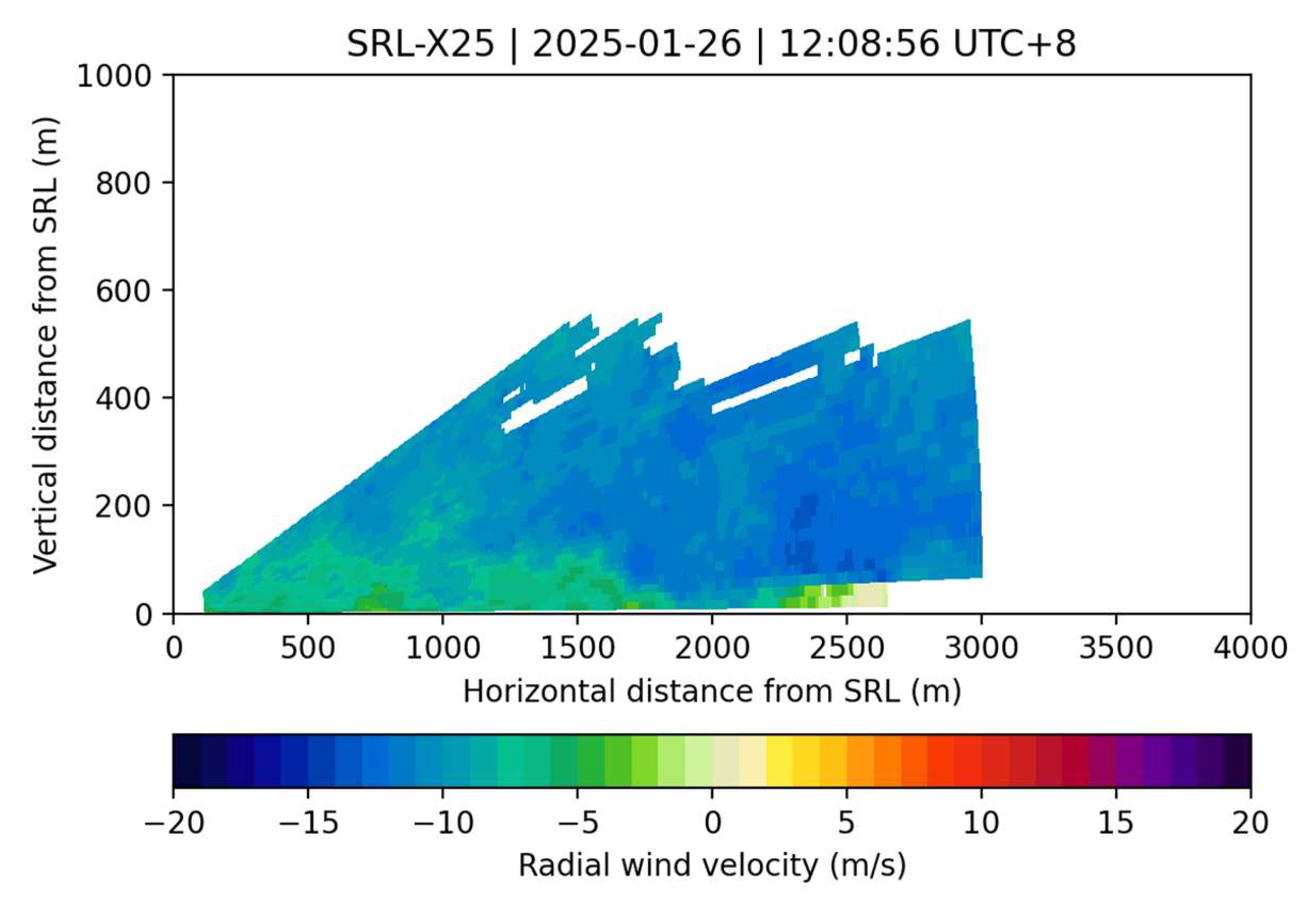
The SRL observation is shown in Figure 11. After flowing over the new terminal building, there was a descending northerly jet (around 13 m/s), reaching the ground at the position of around 2000 m downstream of the SRL. The flow then lifted up, and descended on the ground again at around 1000 m downstream of the SRL. Beneath the jet, the northerly winds were weaker. There was a clear wave structure in the Doppler velocity image of the SRL RHI scan. This behavior differs from terrain-induced disturbances previously documented at HKIA, which are typically tied to larger-scale topography and extend over longer horizontal scales [34].
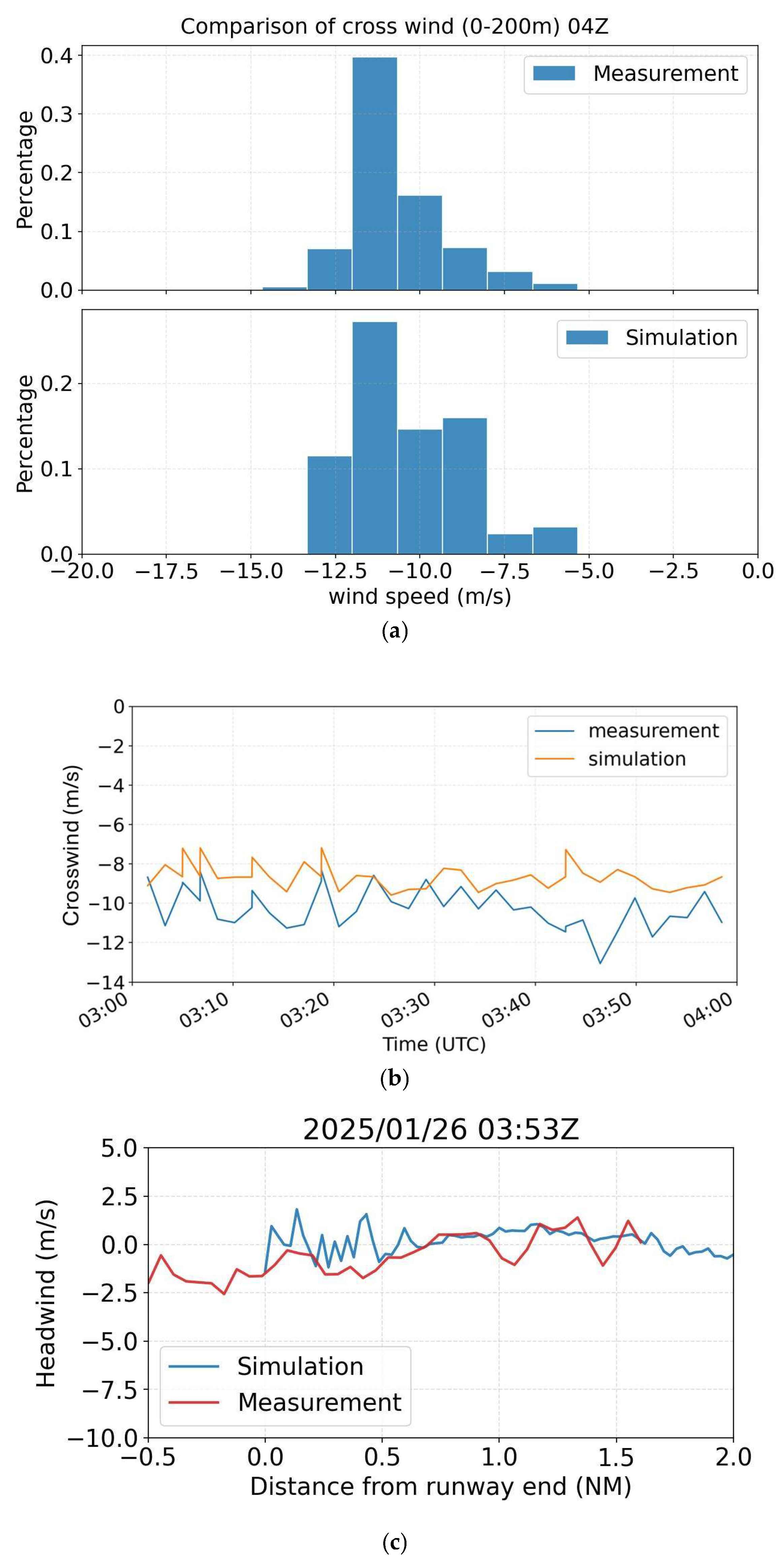
The simulation results were compared with the SRL observations. For the crosswind in the 0–200 m layer (Figure 12a), the simulated distribution agreed well with the measurements, with both datasets showing peaks at around −12 to −10 m/s. The simulated distribution was slightly broader, indicating a wider range of crosswind values. The crosswind time series (Figure 12b) captured the mean magnitude with a slight positive bias and weaker short-term fluctuations than observed. The RMSE and mean bias were 1.91 m s−1 and 1.58 m s−1, respectively. On the other hand, the headwind comparison was good for the two sets of data (Figure 12c), with an RMSE of 1.04 m s−1 and a mean bias of 0.56 m s−1.
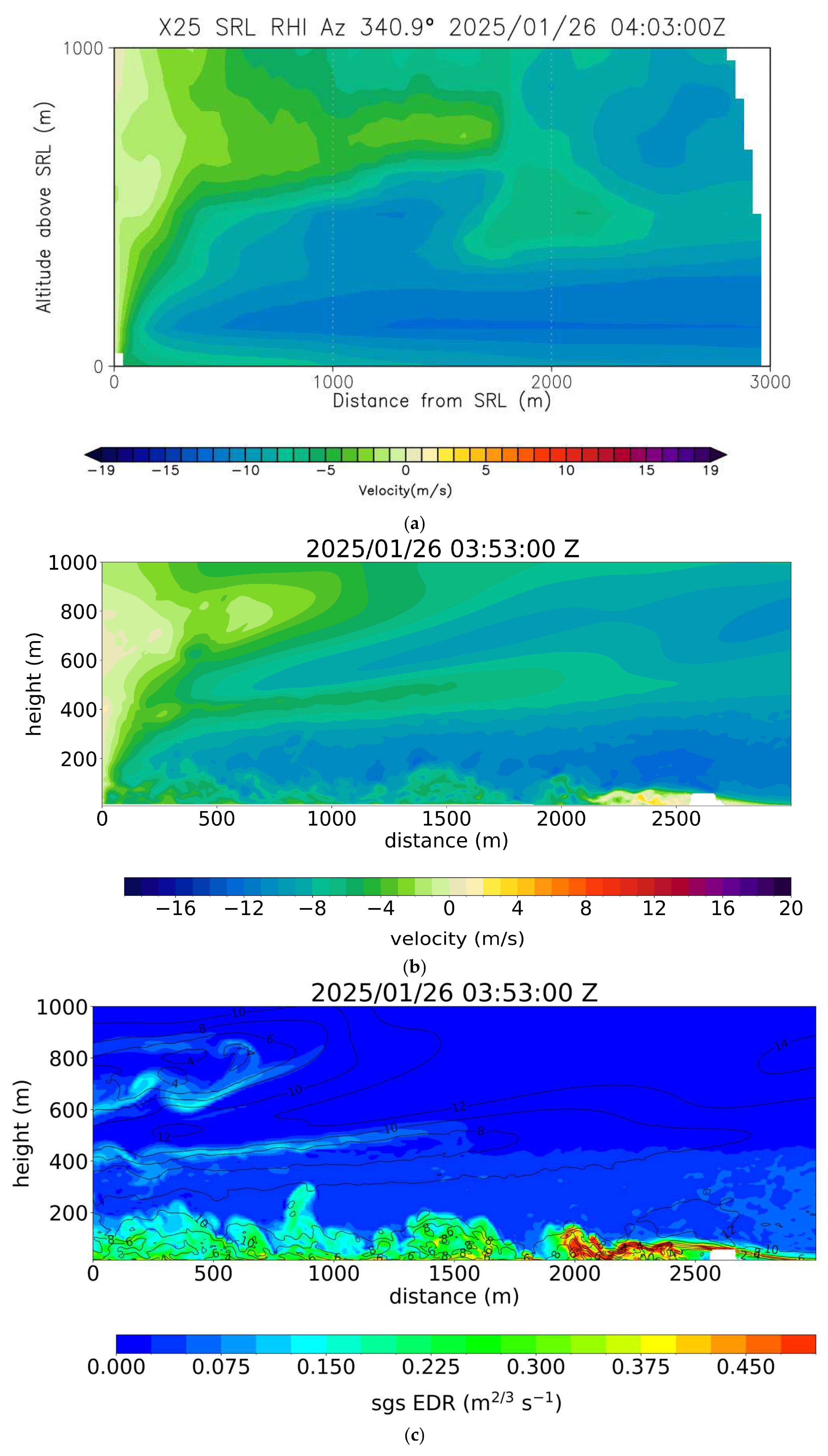
To establish the reason for the wave, the RAMS output was shown in Figure 13a and no wave was observed there. So, the wave may be related to airflow disruption by the building. In fact, for the point upstream of the new terminal building, the potential temperature profile in the simulation (Figure 14) suggested that the atmospheric boundary layer was unstable below a height of around 100 m ( N 2 = 4.64 × 10 5   s 2 at 50 m) with stable condition aloft (from around 200 m upward, N 2 = 9.09 × 10 5   s 2 at 350 m). Such a capped stratification provided a buoyancy restoring force above the near-surface unstable layer and was conducive to a coherent oscillatory response when the flow was perturbed by the building. The simulated RHI scan from PALM (Figure 13b) indeed showed a clear wave structure in the airflow. At the locations of the weaker winds beneath the wave crests, the EDR values are higher (Figure 13c) and the flow is more turbulent. This may have impact on aircraft operation, for both arrival at 25CA and departure at 07CD.
The two case studies showed that the behavior of the building-induced airflow disturbances could be very different. This may partly be related to the stability “background” atmospheric boundary layer. The stability is sensitive to a number of issues, such as the Foehn effect of airflow blowing over the terrain northeast of HKIA, solar heating over the sea/land surface upstream of the new terminal building, as well as mesoscale meteorological processes. Data are being collected by the SRL at X25 and more cases will be reported in the future in order to find out the sensitivity of the building-induced aircraft disturbances to the “background” atmospheric conditions.

4. Conclusions

With the installation of more LIDARs at HKIA, more knowledge is gained about the building-induced airflow disturbances, the so-called low-level wind effect, at this airport. In the present paper, two northerly wind cases have been studied in detail, using SRL observations and CFD simulations driven by a mesoscale meteorological model. It was found that the building-induced disturbance can occur in two characteristic regimes: a simply disturbed flow and a more coherent, wave-like disturbance (a “building-induced wave”). These regimes are closely linked to the stability structure of the background atmospheric boundary layer. The wave-like regime is favored when an unstable near-surface layer is overlaid with a stably stratified layer, which supports the formation and downstream persistence of organized oscillations, whereas a more weakly stratified profile favors a pure turbulence response without coherent structures.
The comparison with SRL observations indicates that the CFD simulations reproduce the primary spatial structures and the downstream extent of the disturbances in both cases, supporting the use of PALM as a diagnostic tool for interpreting the observed low-level wind effects. Nevertheless, noticeable discrepancies remain in the detailed amplitude and fine-scale variability of the SRL signatures, highlighting uncertainties associated with boundary conditions from the mesoscale model, and inflow turbulence representation.
As CFD modelling is costly, the current framework is not yet ready for a real-time operational run. Nevertheless, it could support operations in an offline/forecast-guidance role (e.g., scenario-based simulations under representative stability regimes) and can help interpret LIDAR observations for earlier awareness of potential disturbed-flow conditions affecting runway operations.
A key scientific outcome of the two events is that the occurrence and persistence of coherent building-induced disturbances are highly sensitive to the stability of the upstream atmospheric boundary layer. While this stability dependence is physically plausible and consistent with the observations and simulations presented here, it is inferred from two case studies and therefore may not be fully generalizable; additional events are needed to quantify its robustness and range of applicability.
More cases are being accumulated using SRL observational data. HKIA provides valuable data for examining the interaction of terrain/building with the airflow. Such experience could be useful for the future planning of airports elsewhere in the world. The stability dependence of building-induced airflow disturbances implies that airport wind-hazard assessment and mitigation should also consider representative stability regimes when evaluating building layout, runway-corridor exposure, and the placement of remote-sensing systems.

Author Contributions

Conceptualization, P.W.C.; Methodology, K.W.L. and K.K.L.; Software, K.K.L.; Formal analysis, K.W.L. and Y.D.; Investigation, P.W.C.; Resources, P.C.; Data curation, P.C.; Writing—original draft, P.W.C. All authors have read and agreed to the published version of the manuscript.

Funding

This research received no external funding.

Institutional Review Board Statement

Not applicable.

Informed Consent Statement

Not applicable.

Data Availability Statement

The raw data supporting the conclusions of this article will be made available by the authors on request.

Conflicts of Interest

The authors declare no conflict of interest.

References

  1. Coceal, O.; Dobre, A.; Thomas, T.G. Unsteady Dynamics and Organized Structures from DNS over an Idealized Building Canopy. Int. J. Climatol. 2007, 27, 1943–1953. [Google Scholar] [CrossRef]
  2. Hertwig, D.; Gough, H.L.; Grimmond, S.; Barlow, J.F.; Kent, C.W.; Lin, W.E.; Robins, A.G.; Hayden, P. Wake Characteristics of Tall Buildings in a Realistic Urban Canopy. Bound. Layer Meteorol. 2019, 172, 239–270. [Google Scholar] [CrossRef]
  3. Yeo, H.; Lee, S. Impact of Heterogeneous Building Arrangement on Local Turbulence Escalation. Build. Environ. 2023, 236, 110217. [Google Scholar] [CrossRef]
  4. Southgate-Ash, C.; Mishra, A.; Grimmond, S.; Robins, A.; Placidi, M. Wake Characteristics of Multiscale Buildings in a Turbulent Boundary Layer. Bound. Layer Meteorol. 2025, 191, 20. [Google Scholar] [CrossRef]
  5. Shin, H.H.; Muñoz-Esparza, D.; Sauer, J.A.; Steiner, M. Large-Eddy Simulations of Stability-Varying Atmospheric Boundary Layer Flow over Isolated Buildings. J. Atmos. Sci. 2021, 78, 1487–1501. [Google Scholar] [CrossRef]
  6. Kastner-Klein, P.; Fedorovich, E.; Rotach, M.W. A Wind Tunnel Study of Organised and Turbulent Air Motions in Urban Street Canyons. J. Wind Eng. Ind. Aerodyn. 2001, 89, 849–861. [Google Scholar] [CrossRef]
  7. Carpentieri, M.; Hayden, P.; Robins, A.G. Wind Tunnel Measurements of Pollutant Turbulent Fluxes in Urban Intersections. Atmos. Env. 2012, 46, 669–674. [Google Scholar] [CrossRef]
  8. Li, W.; Mak, C.M.; Cai, C.; Fu, Y.; Tse, K.T.; Niu, J. Wind Tunnel Measurement of Pedestrian-Level Gust Wind Flow and Comfort around Irregular Lift-up Buildings Within Simplified Urban Arrays. Build. Environ. 2024, 256, 111487. [Google Scholar] [CrossRef]
  9. Hadane, A.; Redford, J.A.; Gueguin, M.; Hafid, F.; Ghidaglia, J.-M. CFD Wind Tunnel Investigation for Wind Loading on Angle Members in Lattice Tower Structures. J. Wind Eng. Ind. Aerodyn. 2023, 236, 105397. [Google Scholar] [CrossRef]
  10. Tominaga, Y. CFD Simulations of Turbulent Flow and Dispersion in Built Environment: A Perspective Review. J. Wind Eng. Ind. Aerodyn. 2024, 249, 105741. [Google Scholar] [CrossRef]
  11. Zhang, X.; Weerasuriya, A.U.; Zhang, X.; Tse, K.T.; Lu, B.; Li, C.Y.; Liu, C.-H. Pedestrian Wind Comfort near a Super-Tall Building with Various Configurations in an Urban-like Setting. Build. Simul. 2020, 13, 1385–1408. [Google Scholar] [CrossRef]
  12. Nieuwpoort, A.M.H.; Gooden, J.H.M.; de Prins, J.L. Wind Criteria Due to Obstacles at and Around Airports; NLR-CR-2006-261; National Aerospace Laboratory NLR: Amsterdam, The Netherlands, 2010. [Google Scholar]
  13. Chan, P.W. Generation of an Eddy Dissipation Rate Map at the Hong Kong International Airport Based on Doppler Lidar Data. J. Atmos. Ocean. Technol. 2011, 28, 37–49. [Google Scholar] [CrossRef]
  14. Zhang, H.; Wu, S.; Wang, Q.; Liu, B.; Yin, B.; Zhai, X. Airport Low-Level Wind Shear Lidar Observation at Beijing Capital International Airport. Infrared Phys. Technol. 2019, 96, 113–122. [Google Scholar] [CrossRef]
  15. Boilley, A.; Mahfouf, J.-F. Wind Shear over the Nice Côte d’Azur Airport: Case Studies. Nat. Hazards Earth Syst. Sci. 2013, 13, 2223–2238. [Google Scholar] [CrossRef]
  16. Yoshino, K. Low-Level Wind Shear Induced by Horizontal Roll Vortices at Narita International Airport, Japan. J. Meteorol. Soc. Jpn. Ser. II 2019, 97, 403–421. [Google Scholar] [CrossRef]
  17. Krüs, H.W.; Haanstra, J.O.; van der Ham, R.; Schreur, B.W. Numerical Simulations of Wind Measurements at Amsterdam Airport Schiphol. J. Wind Eng. Ind. Aerodyn. 2003, 91, 1215–1223. [Google Scholar] [CrossRef]
  18. Neofytou, P.; Venetsanos, A.G.; Vlachogiannis, D.; Bartzis, J.G.; Scaperdas, A. CFD Simulations of the Wind Environment around an Airport Terminal Building. Environ. Model. Softw. 2006, 21, 520–524. [Google Scholar] [CrossRef]
  19. Li, L.; Chan, P.W. Numerical Simulation Study of the Effect of Buildings and Complex Terrain on the Low-Level Winds at an Airport in Typhoon Situation. Meteorol. Z. 2012, 21, 183–192. [Google Scholar] [CrossRef]
  20. Lo, K.W.; Hon, K.K.; Chan, P.W.; Li, L.; Li, Q.S. Simulation of Building-Induced Airflow Disturbances in Complex Terrain Using Meteorological-CFD Coupled Model. Meteorol. Z. 2022, 31, 317–330. [Google Scholar] [CrossRef]
  21. Smagorinsky, J. General circulation experiments with the primitive equations: I. The basic experiment. Mon. Weather Rev. 1963, 91, 99–164. [Google Scholar] [CrossRef]
  22. Deardorff, J.W. Stratocumulus-Capped Mixed Layers Derived from a Three-Dimensional Model. Bound. Layer Meteorol. 1980, 18, 495–527. [Google Scholar] [CrossRef]
  23. Maronga, B.; Banzhaf, S.; Burmeister, C.; Esch, T.; Forkel, R.; Fröhlich, D.; Fuka, V.; Gehrke, K.F.; Geletič, J.; Giersch, S.; et al. Overview of the PALM Model System 6.0; Copernicus Publications: Göttingen, Germany, 2020; Volume 13. [Google Scholar]
  24. Raasch, S.; Schröter, M. PALM—A Large-Eddy Simulation Model Performing on Massively Parallel Computers. Meteorol. Z. 2001, 10, 363–372. [Google Scholar] [CrossRef]
  25. Maronga, B.; Gryschka, M.; Heinze, R.; Hoffmann, F.; Kanani-Sühring, F.; Keck, M.; Ketelsen, K.; Letzel, M.O.; Sühring, M.; Raasch, S. The Parallelized Large-Eddy Simulation Model (PALM) Version 4.0 for Atmospheric and Oceanic Flows: Model Formulation, Recent Developments, and Future Perspectives. Geosci. Model. Dev. 2015, 8, 2515–2551. [Google Scholar] [CrossRef]
  26. Žuvela-Aloise, M.; Hahn, C.; Hollósi, B. Evaluation of City-Scale PALM Model Simulations and Intra-Urban Thermal Variability in Vienna, Austria Using Operational and Crowdsourced Data. Urban Clim. 2025, 59, 102245. [Google Scholar] [CrossRef]
  27. Gronemeier, T.; Surm, K.; Harms, F.; Leitl, B.; Maronga, B.; Raasch, S. Evaluation of the Dynamic Core of the PALM Model System 6.0 in a Neutrally Stratified Urban Environment: Comparison between LES and Wind-Tunnel Experiments. Geosci. Model Dev. 2021, 14, 3317–3333. [Google Scholar] [CrossRef]
  28. Resler, J.; Eben, K.; Geletič, J.; Krč, P.; Rosecký, M.; Sühring, M.; Belda, M.; Fuka, V.; Halenka, T.; Huszár, P.; et al. Validation of the PALM Model System 6.0 in a Real Urban Environment: A Case Study in Dejvice, Prague, the Czech Republic. Geosci. Model Dev. 2021, 14, 4797–4842. [Google Scholar] [CrossRef]
  29. Wicker, L.J.; Skamarock, W.C. Time-Splitting Methods for Elastic Models Using Forward Time Schemes. Mon. Weather Rev. 2002, 130, 2088–2097. [Google Scholar] [CrossRef]
  30. Williamson, J.H. Low-Storage Runge-Kutta Schemes. J. Comput. Phys. 1980, 35, 48–56. [Google Scholar] [CrossRef]
  31. Xie, Z.-T.; Castro, I.P. Efficient Generation of Inflow Conditions for Large Eddy Simulation of Street-Scale Flows. Flow Turbul. Combust. 2008, 81, 449–470. [Google Scholar] [CrossRef]
  32. Kim, Y.; Castro, I.P.; Xie, Z.-T. Divergence-Free Turbulence Inflow Conditions for Large-Eddy Simulations with Incompressible Flow Solvers. Comput. Fluids 2013, 84, 56–68. [Google Scholar] [CrossRef]
  33. Chan, P.W.; Cheung, P.; Lai, K.K. Observation and Numerical Simulation of Terrain-Induced Airflow Leading to Low Level Windshear at the Hong Kong International Airport Based on Range-Height-Indicator Scans of a LIDAR. Meteorol. Z. 2024, 33, 255–262. [Google Scholar] [CrossRef]
  34. Chan, P.; Cheung, P.; Chong, M.; Lai, K. New Observations of Airflow at Hong Kong International Airport by Range Height Indicator (RHI) Scans of LIDARs and Their Numerical Simulation. Appl. Sci. 2025, 15, 9655. [Google Scholar] [CrossRef]
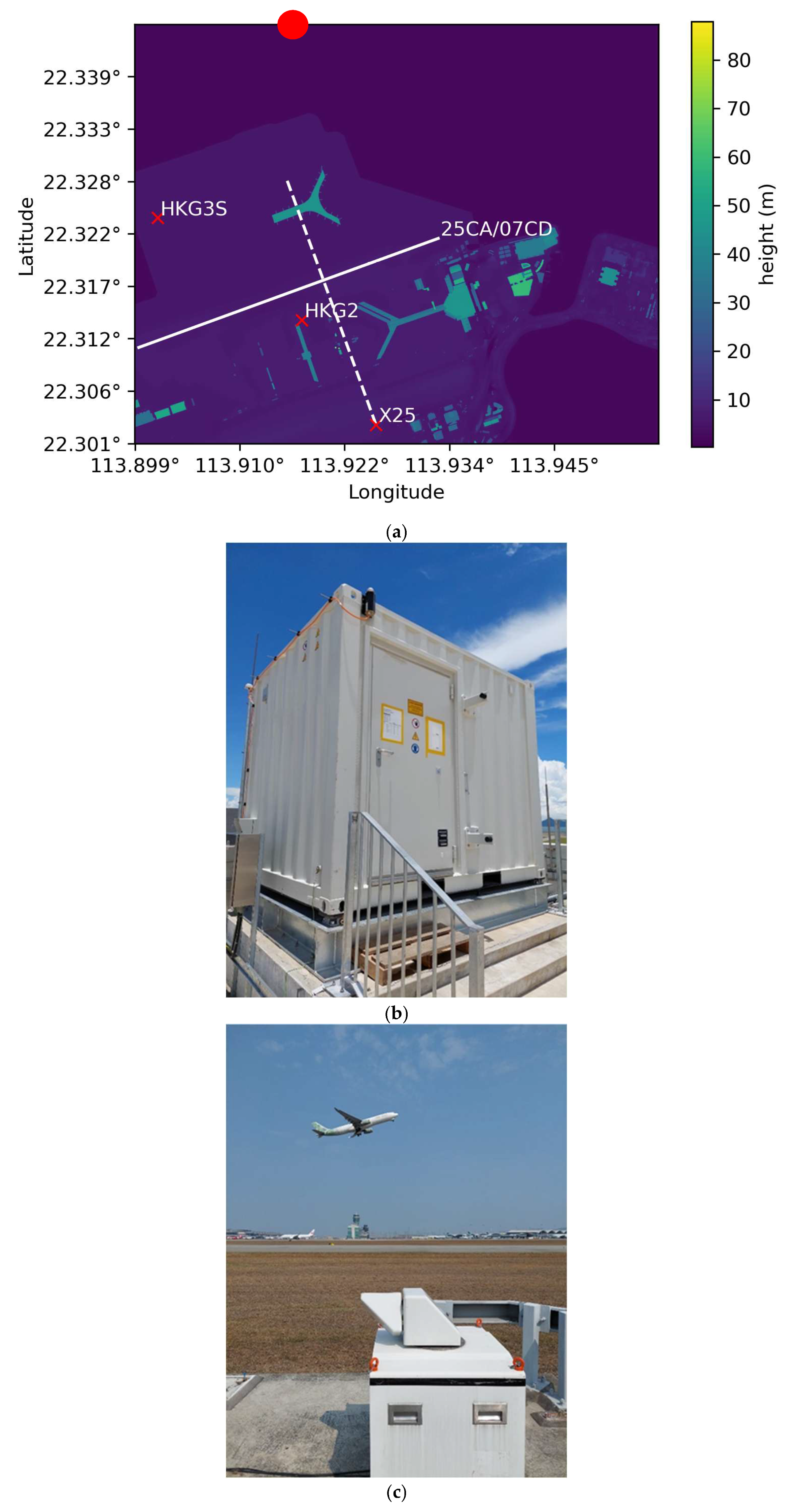
Figure 1. (a) Domain of PALM simulation, colored by height above mean sea level. The location of the LRLs (HKG3S and HKG2) and SRL (X25) are indicated by red star symbols. The runway corridor 25CA/07CD is indicated by a white solid line. The plane of the RHI scan from the SRL is indicated by a white dashed line. The red dot is the position at which the potential temperature profile of the RAMS simulation is extracted. (b) Photo of the LRL near the north runway, HKG3S. (c) Photo of SRL X25.
Applsci 16 00404 g001
Figure 2. (a) The first, second, and third nested domains of the RAMS simulation. (b) The third, fourth, and fifth nested domains of the RAMS simulation. (c) The domain of the PALM simulation denoted by a red rectangle where the boundary is the fifth nested domain of the RAMS simulation.
Applsci 16 00404 g002
Figure 3. LIDAR plan-position indicator scan on 15 January 2025, 01:25 UTC. (a) Doppler velocity and (b) EDR.
Applsci 16 00404 g003
Figure 4. SRL range-height indicator scan on (a) 15 January 2025, 01:15 UTC, and (b) 15 January 2025, 01:52 UTC.
Applsci 16 00404 g004
Figure 5. Comparison of observations and PALM simulations on 15 January 2025: (a) distribution of crosswind at the intersection of the SRL RHI plane and runway 25CA/07CD from 0 to 100 m above ground, and (b) headwind profile along runway 25CA/07CD. (c) Time series of crosswind at the intersection of the SRL RHI plane and runway 25CA/07CD at a height of about 50 m above ground.
Applsci 16 00404 g005
Figure 6. Simulated SRL range-height indicator scan from RAMS on (a) 15 January 2025, 01:22 UTC, and (b) 15 January 2025, 01:25 UTC.
Applsci 16 00404 g006
Figure 7. Simulated SRL range-height indicator scan from PALM on (a) 15 January 2025, 01:15 UTC, and (b) 15 January 2025, 01:52 UTC.
Applsci 16 00404 g007
Figure 8. Time evolution of sub-grid-scale eddy dissipation rate from the PALM simulation on 15 January 2025: (a) 01:01 UTC, (b) 01:04 UTC, and (c) 01:09 UTC.
Applsci 16 00404 g008
Figure 9. Potential temperature profiles upstream of the new terminal on 15 January 2025: (a) 01:22 UTC and (b) 01:25 UTC.
Applsci 16 00404 g009
Figure 10. LIDAR plan-position indicator scan on 26 January 2025: (a) Doppler velocity at 04:02 UTC, and (b) EDR at 04:11 UTC.
Applsci 16 00404 g010
Figure 11. SRL range-height indicator scan on 26 January 2025, 04:08 UTC.
Applsci 16 00404 g011
Figure 12. Comparison of observations and PALM simulations on 26 January 2025: (a) distribution of crosswind at the intersection of the SRL RHI plane and runway 25CA/07CD from 0 to 200 m above ground. (b) Time series of crosswind at the intersection of the SRL RHI plane and runway 25CA/07CD at a height of about 50 m above ground. (c) Headwind profile along runway 25CA/07CD.
Applsci 16 00404 g012
Figure 13. (a) Simulated SRL range-height indicator scan from RAMS on 26 January 2025, 04:03 UTC. (b) Simulated SRL range-height indicator scan from PALM on 26 January 2025, 03:53 UTC. (c) Sub-grid-scale eddy dissipation rate from the PALM simulation at the same time with contours of velocity magnitude.
Applsci 16 00404 g013
Figure 14. Potential temperature profiles upstream of the new terminal on 26 January 2025, 04:03 UTC.
Applsci 16 00404 g014
Disclaimer/Publisher’s Note: The statements, opinions and data contained in all publications are solely those of the individual author(s) and contributor(s) and not of MDPI and/or the editor(s). MDPI and/or the editor(s) disclaim responsibility for any injury to people or property resulting from any ideas, methods, instructions or products referred to in the content.