Article

Optimal Cell Segmentation and Counting Strategy for Embedding in Low-Power AIoT Devices

Department of Smart Automotive, Soonchunhyang University, 22 Soonchunhyang-ro, Sinchang-myeon, Asan-si 31538, Chungcheongnam-do, Republic of Korea
*
Author to whom correspondence should be addressed.
Appl. Sci. 2026, 16(1), 357; https://doi.org/10.3390/app16010357 (registering DOI)
Submission received: 9 November 2025 / Revised: 19 December 2025 / Accepted: 27 December 2025 / Published: 29 December 2025
(This article belongs to the Special Issue Advanced Intelligent Technologies in Bioinformatics and Biomedicine)

Abstract

This study proposes an end-to-end (E2E) optimization methodology for a white blood cell (WBC) cell segmentation and counting (CSC) pipeline with a focus on deployment to low-power Artificial Intelligence of Things (AIoT) devices. The proposed framework addresses not only the selection of the segmentation model but also the corresponding loss function design, watershed threshold optimization for cell counting, and model compression strategies to balance accuracy, latency, and model size in embedded AIoT applications. For segmentation model selection, UNet, UNet++, ResUNet, EffUNet, FPN, BiFPN, PFPN, Cell-ViT, Evit-UNet and MAXVitUNet were employed, and three types of loss functions—binary cross-entropy (BCE), focal loss, and Dice loss—were utilized for model training. For cell-counting accuracy optimization, a distance transform-based watershed algorithm was applied, and the optimal threshold value was determined experimentally to lie within the range of 0.4 to 0.9. Quantization and pruning techniques were also considered for model compression. Experimental results demonstrate that using an FPN model trained with focal loss and setting the watershed threshold to 0.65 yields the optimal configuration. Compared to the latest baseline techniques, the proposed CSC E2E pipeline achieves a 21.1% improvement in cell-counting accuracy while reducing model size by 74.5% and latency by 16.8% through model compression. These findings verify the effectiveness of the proposed optimization strategy as a lightweight and efficient solution for real-time biomedical applications on low-power AIoT devices.

1. Introduction

Accurate segmentation and counting of white blood cells (WBCs) in peripheral blood smear images play a critical role not only in hematological diagnosis but also in a wide range of clinical and industrial applications, including automated hematology analyzers, tele-hematology platforms, and clinical laboratory automation systems [1,2,3]. Morphological differentiation and quantitative analysis of WBCs provide concentration-related information that serves as a key biomarker for diagnosing and assessing the prognosis of infectious, autoimmune, and hematologic neoplastic diseases. Traditionally, hematologists manually identify and classify cells under a microscope using stained smear slides. However, this process is time-consuming, labor-intensive, and subject to human error and inter-observer variability [4,5]. Such manual dependence not only limits clinical reliability but also reduces scalability for large-population studies and high-throughput biomedical research.
The cell segmentation and counting (CSC) technique has significant industrial potential across various biomedical fields. In clinical laboratories, it enables standardized, rapid, and reproducible diagnostic workflows, thereby reducing the workload of hematologists and minimizing human errors [6]. In digital pathology and tele-hematology, these automated systems provide a foundation for remote diagnostic platforms and deliver substantial value in regions with limited access to specialized hematologists [7]. In the pharmaceutical industry, automated WBC quantification plays an essential role in evaluating drug toxicity and immune responses across large-scale sample cohorts, thereby contributing to drug development pipelines and personalized precision medicine [8]. Integrating AI-based cell segmentation models into automated hematology analyzers holds the potential to transform the healthcare industry by enhancing both clinical utility and economic scalability.
Recent advances in computer vision and artificial intelligence [9,10,11,12,13,14,15,16,17,18,19,20,21,22,23,24,25] have created new opportunities to automate WBC segmentation and counting with improved accuracy and efficiency. Early studies utilized conventional image-processing methods such as thresholding and morphological operations [4,20,21]. However, these methods were sensitive to illumination variations, staining inconsistencies, and cell overlap, making them unreliable in practical clinical environments. In contrast, recent deep learning-based approaches, particularly CNN-based architectures such as U-Net [9], U-Net++ [10], Mask R-CNN [22], and Hover-Net [23], have demonstrated superior pixel-wise segmentation performance compared with rule-based techniques. These models exhibit strong boundary extraction and separation capabilities in overlapping-cell regions, and their performance is commonly evaluated using metrics such as Dice coefficient, mean intersection over union (mIoU), and sensitivity. Furthermore, recent studies [20,21,24,25] have compared various segmentation networks to identify optimal architectures for cell segmentation. Nevertheless, their performance remains limited, as they focus primarily on segmentation without incorporating counting.
However, optimizing segmentation accuracy alone does not necessarily guarantee reliable cell counting performance, as errors in boundary precision and instance separation can propagate and be amplified in subsequent counting stages. In practice, segmentation, counting, and deployment constraints are often optimized independently, leading to fragmented pipelines that lack consistency across tasks. This motivates the need for an integrated end-to-end (E2E) optimization framework that jointly considers segmentation quality, counting calibration, and on-device efficiency to ensure robust and deployable CSC performance.
In this paper, we propose an optimization strategy for cell segmentation and counting using the WBC dataset [26] and Chinese Hamster Ovary (CHO) cell [27], and we further present a deep learning-based model compression strategy for commercialization in biomedical diagnostic systems. The proposed optimization framework achieves state-of-the-art (SOTA) segmentation and counting performance while maintaining high model efficiency optimized for low-power AIoT deployment.
The primary contributions of this study are summarized as follows:
  • Optimization of Cell Segmentation: This study presents a performance optimization strategy for cell segmentation by evaluating various data augmentation techniques, segmentation backbones, and loss functions. The proposed approach enhances segmentation performance in terms of accuracy, Dice coefficient, sensitivity, and mIoU.
  • Optimization of the End-to-End CSC Pipeline: To improve the accuracy of the CSC pipeline, multiple segmentation models and distance transform-based watershed threshold configurations were compared. Through this analysis, the optimal combination of segmentation and counting techniques for the CSC E2E pipeline was derived.
  • Model Lightening and AIoT Deployment Optimization: A model lightening methodology was proposed to enable efficient deployment on low-power AIoT devices. This includes strategies for balancing accuracy, latency, and model size to achieve optimal performance under hardware-constrained environments.

2. Related Works

Early studies on cell segmentation primarily relied on image preprocessing and morphological operations. Techniques such as Otsu thresholding, K-means clustering, and the watershed transform were widely adopted to separate nuclei and cytoplasm based on staining intensity differences [4,5]. However, these conventional methods are highly sensitive to illumination non-uniformity, staining variability, and overlapping cells in smear images, making it difficult to ensure consistent segmentation performance in clinical environments [20].
In recent years, data-driven cell segmentation approaches based on convolutional neural networks (CNNs) [9,10,22,25] have achieved remarkable progress. Among them, UNet [9] demonstrated outstanding performance in biomedical image segmentation through its symmetric encoder–decoder architecture, while UNet++ [10,25] improved boundary restoration by introducing nested and dense skip connections. Mask R-CNN [22] extended object detection frameworks to instance-level segmentation, enabling cell-wise prediction within complex scenes. More recently, Transformer-based models [16] have been introduced to overcome the locality limitation of CNNs. Models such as CellViT [17], EvitUNet [18] and MaxVitUNet [19] leverage a self-attention mechanism to capture global structural relationships among cells, achieving robust segmentation, even under low-contrast or highly overlapped conditions. These approaches have demonstrated improved accuracy over CNN-based methods, particularly in challenging overlapping or densely packed cell regions.
Traditionally, cell counting has been performed using blob detection or watershed-based centroid localization. However, in high-density or overlapping regions, these methods often suffer from unstable centroid estimation. To address this limitation, density regression-based approaches were proposed. Lempitsky and Zisserman [28] introduced a density map regression technique that models object centers with Gaussian kernels, while CSRNet [29] employed dilated convolutions to enhance counting accuracy in highly congested cellular regions. More recently, end-to-end architectures that jointly perform segmentation and counting have emerged. These models learn both the segmentation decoder and the density regression head simultaneously, achieving consistent optimization between pixel-level and instance-level predictions [30]. In particular, multi-task learning frameworks have been shown to improve both boundary accuracy in segmentation and quantitative precision in counting by enabling mutual feature sharing between tasks.
Recent advances in cell segmentation have increasingly focused on foundation models and label-efficient learning strategies to improve generalization across diverse microscopy conditions. Study [31] introduced Segment Anything for Microscopy (μSAM), which adapts the Segment Anything Model (SAM) to both light and electron microscopy through domain-specific fine-tuning. By unifying interactive and automatic segmentation within a single framework, μSAM demonstrated competitive or superior performance compared to CellPose and traditional microscopy tools across multiple datasets and modalities Similarly, CellSAM [32] extended the foundation-model paradigm to cell segmentation by leveraging large-scale pretraining, enabling robust segmentation under limited annotation scenarios and heterogeneous imaging conditions. In parallel, recent studies [33] on unsupervised cell instance segmentation have explored object-centric embedding learning, allowing accurate separation of individual cells without pixel-level supervision. Such approaches significantly reduce annotation costs while maintaining competitive segmentation accuracy. Collectively, these works indicate a clear trend toward foundation models and self-supervised learning as key enablers for scalable and generalizable cell segmentation systems.
Despite these advancements, most existing studies are limited to dataset-specific optimization and lack sufficient validation under domain shift conditions. Furthermore, visual uncertainty factors in microscopic imagery—such as staining variations, defocus blur, and overlapping cells—remain largely unaddressed. Furthermore, foundation model-based and unsupervised learning methods typically require large model capacities in the absence of explicit labels, which leads to increased computational and memory demands, thereby limiting their applicability to low-power IoT devices.
In parallel, model optimization for lightweight and real-time inference has become an increasingly important research direction. In medical imaging, reducing model size and computational complexity is essential for on-device inference in embedded or portable systems. Quantization and pruning techniques [34] are representative approaches for model compression, reducing both parameter size and FLOPs by applying fixed-point arithmetic or eliminating redundant weights. More recent studies leverage Knowledge Distillation (KD) [35] and Neural Architecture Search (NAS) [36] to automatically discover efficient architectures that preserve accuracy while being suitable for deployment on embedded AI hardware. These strategies provide the technological foundation for implementing real-time cell segmentation and counting models in low-power edge devices such as clinical microscopes and portable hematology analyzers.

3. System Model

Figure 1 illustrates the proposed methodology for optimizing the end-to-end (E2E) cell segmentation and counting (CSC) pipeline designed for low-power AIoT devices. The overall optimization process consists of three sequential stages: cell segmentation, cell counting, and model compression.

3.1. Cell Segmentation

3.1.1. Segmentation Model Selection

For the cell segmentation task, various encoder–decoder-based deep neural networks were considered, including the UNet family—UNet [9], UNet++ [10], and ResUNet [11]—as well as an EfficientNet-based variant (EffUNet) [12]. Additionally, feature pyramid network (FPN) structures such as FPN [13], BiFPN [14], and PFPN [15], and transformer-based architectures including CellViT [17], EvitUNet [18] and MaxVitUNet [19] were employed for performance comparison.
Although all models share an encoder–decoder backbone structure, their feature extraction mechanisms and skip-connection strategies lead to distinct representational capacities and computational efficiencies. The baseline UNet [9] employs a symmetric encoder–decoder architecture that effectively reconstructs clear boundaries between nuclei and cytoplasm. UNet++ [10], built upon DenseNet [37], introduces dense skip connections to enhance multi-scale feature fusion between encoder and decoder, thereby improving boundary delineation among adjacent cells. ResUNet [11] incorporates residual connections to mitigate the gradient vanishing problem in deep neural networks and to achieve robust representation learning under morphological discontinuities or staining inconsistencies. EffUNet combines an EfficientNet encoder with a UNet decoder to provide computationally efficient segmentation performance optimized for embedded AI applications.
The FPN [13] and BiFPN [14] architectures utilize feature pyramid structures to jointly capture high-resolution cell structures and low-resolution global context. BiFPN further refines this approach using bidirectional feature fusion, enhancing efficiency in feature aggregation and providing robust segmentation performance in blood smear images with variable cell size and shape. PFPN [15] adds a pyramid attention mechanism that assigns spatially adaptive weights, enabling better differentiation between cellular centers and boundary regions.
Recently, transformer-based segmentation models such as CellViT [17], EvitUNet [18], and MaxVitUNet [19] have gained attention for their ability to learn global contextual relationships among cells via self-attention. CellViT adopts a hybrid structure combining a Vision Transformer and a CNN backbone to simultaneously capture local morphology and global context. EvitUNet introduces an efficient token-reduction mechanism to lower the computational complexity of the transformer while maintaining precise boundary recognition. MaxViT-UNet represents a lightweight UNet-based medical image segmentation framework that incorporates multi-axis attention into both the encoder and decoder, effectively combining local convolutional representations with global Transformer-based contextual modeling.
These architectures, each with distinct structural characteristics, were evaluated under identical dataset and experimental conditions to determine the optimal model for the cell segmentation task in terms of accuracy, complexity, and training efficiency. All models were trained using the same preprocessing pipeline, hyperparameters, and three loss functions—binary cross entropy (BCE) [38], Dice loss [39], and focal loss [40]—and were evaluated with Dice coefficient, mIoU, precision, and recall metrics.
To further clarify the rationale behind the segmentation model selection, the considered architectures were intentionally chosen to represent diverse design philosophies along three key dimensions: feature fusion strategy, contextual modeling capability, and computational efficiency. UNet-based models emphasize precise spatial localization through skip connections, making them suitable for delineating fine cellular boundaries in microscopy images. FPN-based models extend this capability by explicitly modeling multi-scale representations, which is particularly effective in blood smear images where cell sizes and shapes vary significantly. In contrast, transformer-based models aim to capture long-range dependencies and global context via self-attention, which can be advantageous in dense or overlapping cell regions. However, such global modeling often incurs higher computational cost and memory overhead. By systematically evaluating these heterogeneous architectures under identical experimental conditions, this study aims to provide a comprehensive analysis of how different architectural choices impact segmentation accuracy, boundary sensitivity, and deployment feasibility on low-power AIoT devices. This comparative design enables a principled selection of segmentation models that balance accuracy and efficiency within an end-to-end CSC pipeline.

3.1.2. Training Loss Selection

For training the aforementioned segmentation models, three loss functions were employed: BCE, Dice loss, and focal loss. Each loss function targets different aspects of segmentation performance: pixel-level prediction accuracy, class-imbalance correction, and robustness in boundary regions, respectively.
The BCE loss computes pixel-wise cross-entropy between the predicted probability p i and the ground-truth label g i { 0 , 1 } , enforcing discrimination between cell (positive) and background (negative) pixels:
L BCE = 1 N i = 1 N g i log ( p i ) + ( 1 g i ) log ( 1 p i )
Although BCE directly reflects prediction confidence, it becomes less effective under severe class imbalance, where positive (cell) regions contribute less to the total loss.
Dice loss measures similarity based on the overlap between prediction and ground-truth masks. Given a predicted mask P and a ground-truth mask G, it is defined as
L Dice = 1 2 i = 1 N p i g i + ϵ i = 1 N p i + i = 1 N g i + ϵ
where ϵ is a small constant for numerical stability. Dice loss effectively compensates for class imbalance and enhances segmentation performance near cell boundaries.
Focal loss extends BCE by reducing the relative loss contribution of well-classified samples and focusing on hard examples [40]. It is formulated as
L Focal = 1 N i = 1 N α ( 1 p i ) γ g i log ( p i ) + ( 1 α ) p i γ ( 1 g i ) log ( 1 p i )
Here, α [ 0 , 1 ] is the weighting factor for the positive class, and γ > 0 is a focusing parameter. A higher γ value reduces the influence of easy samples, forcing the model to learn from difficult ones. In this study, α = 0.25 , γ = 2.0 were adopted.

3.2. Cell Counting

Distance Transform-Based Watershed

To quantify the number of cells, this study applies a distance transform-based watershed algorithm to the cell segmentation result mask. This approach defines the center of each cell as a seed and simulates the spread of water from the center toward the boundary to determine borders between overlapping cells.
Let the cell segmentation result map be represented as M ( x , y ) 0 , 1 . The distance transform D ( x , y ) is defined as the Euclidean distance from each pixel to the nearest cell boundary as follows:
D ( x , y ) = min ( x , y ) M ( x , y ) ( x , y ) 2 ,
where M denotes the set of boundary pixels, and the value of D ( x , y ) reaches its maximum at the cell center.
The local maxima of the distance transform are used as candidates for cell center seeds. However, due to noise or structural variations within cells, unnecessary seeds may be generated. Therefore, in this study, a watershed threshold T w is applied to select valid seeds:
S ( x , y ) = 1 , if D ( x , y ) T w · D max , 0 , otherwise ,
where D max = max ( x , y ) D ( x , y ) , and T w [ 0 , 1 ] is a hyperparameter controlling the density of seed points. A larger T w value reduces the number of seeds, potentially leading to under-segmentation, whereas a smaller T w value may cause over-segmentation.
The watershed algorithm treats the distance map as a topographical elevation model and performs segmentation by simulating the water flooding process. When the distance transform is negated, cell centers correspond to valleys and boundaries to ridges:
H ( x , y ) = D ( x , y )
Then, the seed map S ( x , y ) is used as the initial minima for the watershed operation:
L ( x , y ) = Watershed ( H ( x , y ) , S ( x , y ) )
The final labeled map L ( x , y ) contains unique labels representing individual cells, and the total number of distinct labels N c = | unique ( L ( x , y ) ) | corresponds to the final cell count.
The watershed threshold T w is optimized to minimize the mean absolute error (MAE) between the predicted and ground-truth cell counts:
T w * = arg min T w [ 0 , 1 ] MAE N c ( T w ) , N G T
where N G T denotes the ground-truth cell count.

3.3. Model Compression

To enable lightweight and real-time inference of the cell segmentation model, various model compression techniques were applied. Specifically, considering the trade-off between accuracy, latency, and model size, FP16 quantization, INT8 quantization, and pruning methods were analyzed and compared. Among these, the configuration that achieved the optimal balance between performance and efficiency was selected as the final model.

3.3.1. FP16 Quantization

FP16 Quantization reduces the precision of floating-point operations from 32-bit (FP32) to 16-bit, effectively halving memory consumption while maintaining a comparable dynamic range. FP16 operations are natively supported by GPUs and AI accelerators and can achieve nearly the same inference speed as FP32 while providing roughly a 50% reduction in model size. In this study, FP16 quantization was applied as a post-training quantization procedure using the PyTorch 2.8.0’s native quantization utilities (torch.ao.quantization). Neither quantization-aware training nor additional calibration steps were required, as the numerical range of FP16 sufficiently preserved the distribution of weights and activations in the evaluated models. As a result, the accuracy degradation after quantization remained below 1% across all architectures, confirming that FP16 quantization provides an effective and low-overhead compression strategy for real-time CSC deployment on low-power AIoT devices.

3.3.2. INT8 Quantization

INT8 Quantization converts model weights and activations into 8-bit integers, substantially reducing computation and memory access. In this study, quantization-aware training (QAT) was adopted to integrate the quantization process directly into training. Each layer’s weights w and activations a are scaled as follows:
Q ( w ) = clip round w s w , q min , q max , Q ( a ) = clip round a s a , q min , q max
where s w and s a are scale factors, and q min , q max represent the integer range. Through QAT, quantization-induced error accumulation was minimized, theoretically reducing model size by a factor of four compared to FP32 precision.

3.3.3. Structured Pruning

Pruning eliminates parameters with low contribution to obtain model sparsity and reduce computational cost. In this study, a structured filter pruning method was applied to evaluate filter-level importance. The importance of the k-th filter, α k , is defined by its mean magnitude:
α k = 1 N k i = 1 N k | w k , i | , P = { k α k < τ p }
where τ p denotes the pruning threshold. Filters with lower importance values were removed, followed by fine-tuning of the remaining structure to recover potential performance loss.

4. Experimental Results

The results of the cell segmentation model and training loss methods used for optimizing the CSC E2E pipeline are presented in Table 1. In addition, the optimization results for cell counting are shown in Table 2, and the outcomes of the CSC model compression are summarized in Table 3.
For clarity, the ground truth (GT) used in this study is defined as follows. The GT for cell segmentation was directly obtained from the pixel-wise segmentation annotations provided in the publicly available dataset. For cell counting, the GT values were derived by manually counting individual cells based on the corresponding GT segmentation masks, ensuring consistency between segmentation and counting evaluations. This separation of GT definitions allows a clear and fair assessment of both segmentation accuracy and downstream counting performance within the proposed CSC E2E pipeline.

4.1. Performance Analysis of Cell Segmentation

Table 1 presents the segmentation performance results on the blood cell segmentation dataset, comparing three loss functions: BCE, focal, and dice. The evaluation metrics include accuracy (Acc), Dice coefficient (Dice), sensitivity (Sens), and mean intersection over union (mIoU).
Overall, all models achieve over 97% accuracy, 95% Dice, 93% sensitivity, and 89% mIoU, demonstrating stable segmentation performance across most configurations.
From a loss-function perspective, BCE, focal, and Dice losses all show stable accuracy, Dice coefficient, and sensitivity results, while mIoU performance under focal loss is slightly less stable. Under BCE and Dice losses, most models achieve nearly identical Dice scores, whereas focal loss tends to show slightly lower Dice values (by about 0.2–0.4 on average). This is because focal loss emphasizes hard examples near cell boundaries, providing better boundary discrimination, but since this dataset features relatively balanced blood-cell distributions, its benefits are only partially manifested.
From a model perspective, the UNet family (UNet, UNet++, and ResUNet) consistently achieves the highest accuracy, Dice coefficient, sensitivity, and mIoU values under BCE and Dice losses. Meanwhile, Transformer-based architectures such as CellViT, Evit-UNet and MaxVitUNet, while offering strong global feature representation and better generalization across morphological variations, show slightly lower boundary precision when trained on smaller datasets.
Regarding model size and latency efficiency, FPN and ResUNet perform the best. FPN achieves the smallest model size (16.7 MB) and the fastest inference time (21.5 ms) without any loss of accuracy, making it ideal for real-time applications. ResUNet also provides balanced performance, with a model size of 26.9 MB and latency of 21.5 ms, benefiting from its residual lightweight architecture. In contrast, UNet++ shows higher latency (28.9 ms) due to its multiple skip-path structures, while EffUNet experiences increased latency due to the multi-stage complexity of the Mobile inverted bottleneck convolution (MBConv) in its EfficientNet encoder. Similarly, BiFPN suffers from heavier computation caused by multiple bidirectional feature fusion paths.
In conclusion, UNet, ResUNet, and FPN deliver the most balanced performance, achieving high segmentation accuracy (Dice ≥ 96.5%) and low latency (≤22 ms). Among them, FPN demonstrates the best trade-off between accuracy and efficiency, being particularly suitable for real-time blood-cell segmentation tasks due to its small model size (16.7 MB) and low computation cost.

4.2. Performance Analysis of Cell Counting

Table 2 presents the variation in average cell counting accuracy according to the watershed threshold ( T w ) based on the segmentation results from Table 1. In the table, the highest accuracy per model and threshold setting is highlighted in bold. Since the threshold directly controls seed selection in the distance transform process, lower T w values lead to over-segmentation, while higher values result in under-segmentation. Therefore, the choice of T w significantly affects counting accuracy.
From a loss-function perspective, focal loss consistently achieves the highest counting accuracy. This differs from Table 1, where BCE and Dice losses yielded the best segmentation results, confirming that higher segmentation accuracy does not necessarily translate to higher counting accuracy. This can be attributed to focal loss’s robustness near uneven boundary intensities, which stabilizes seed-map generation in the counting stage.
When examining thresholds, the optimal value T w * varies with the loss function. For BCE Loss, the optimal accuracy occurs around 0.85–0.9; for focal Loss, the optimal accuracy is between 0.55–0.65; and for Dice Loss, optimal accuracy is around 0.7 for all models. This indicates that each loss function requires a distinct threshold tuning strategy for optimal deployment.
This behavior can be further explained by the different boundary characteristics induced by each loss function during segmentation training. BCE and Dice loss tend to produce relatively sharp and high-contrast boundaries between foreground and background regions, which results in distance-transform maps with steep gradients near cell borders. Consequently, higher watershed thresholds are required to suppress spurious local maxima and avoid over-segmentation. In contrast, focal loss emphasizes hard-to-classify pixels near ambiguous or low-contrast boundaries, leading to smoother boundary transitions and more gradual distance-transform gradients. As a result, meaningful cell-center seeds emerge at lower relative distance values, shifting the optimal watershed threshold toward a smaller T w . This observation highlights that watershed threshold sensitivity is intrinsically linked to segmentation boundary sharpness and noise smoothness and therefore must be jointly optimized with the chosen loss function rather than treated as an independent post-processing parameter.
Under the focal loss setting, which yields the best overall performance, a model-wise comparison shows that MaxVitUNet and UNet++ achieve the highest cell counting accuracies of 0.96 and 0.95, respectively. In addition, UNet also demonstrates strong performance, while all other evaluated models consistently achieve stable cell counting accuracy exceeding 0.91 when trained with focal loss.
Therefore, from a pipeline optimization perspective, focal loss is recommended for counting tasks, MaxVitUNet and UNet++ for accuracy-oriented applications, and FPN or ResUNet for efficiency-oriented implementations.
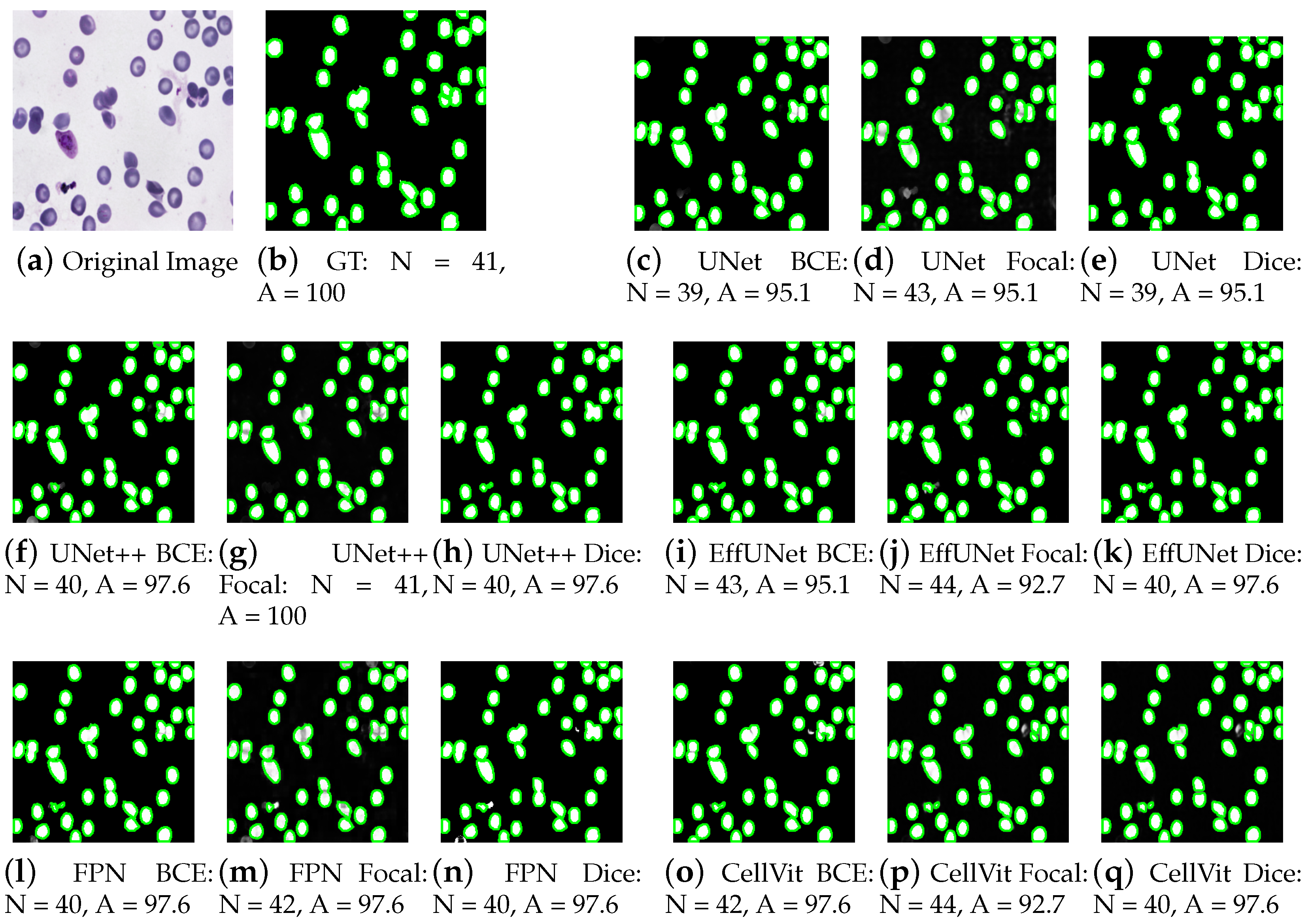
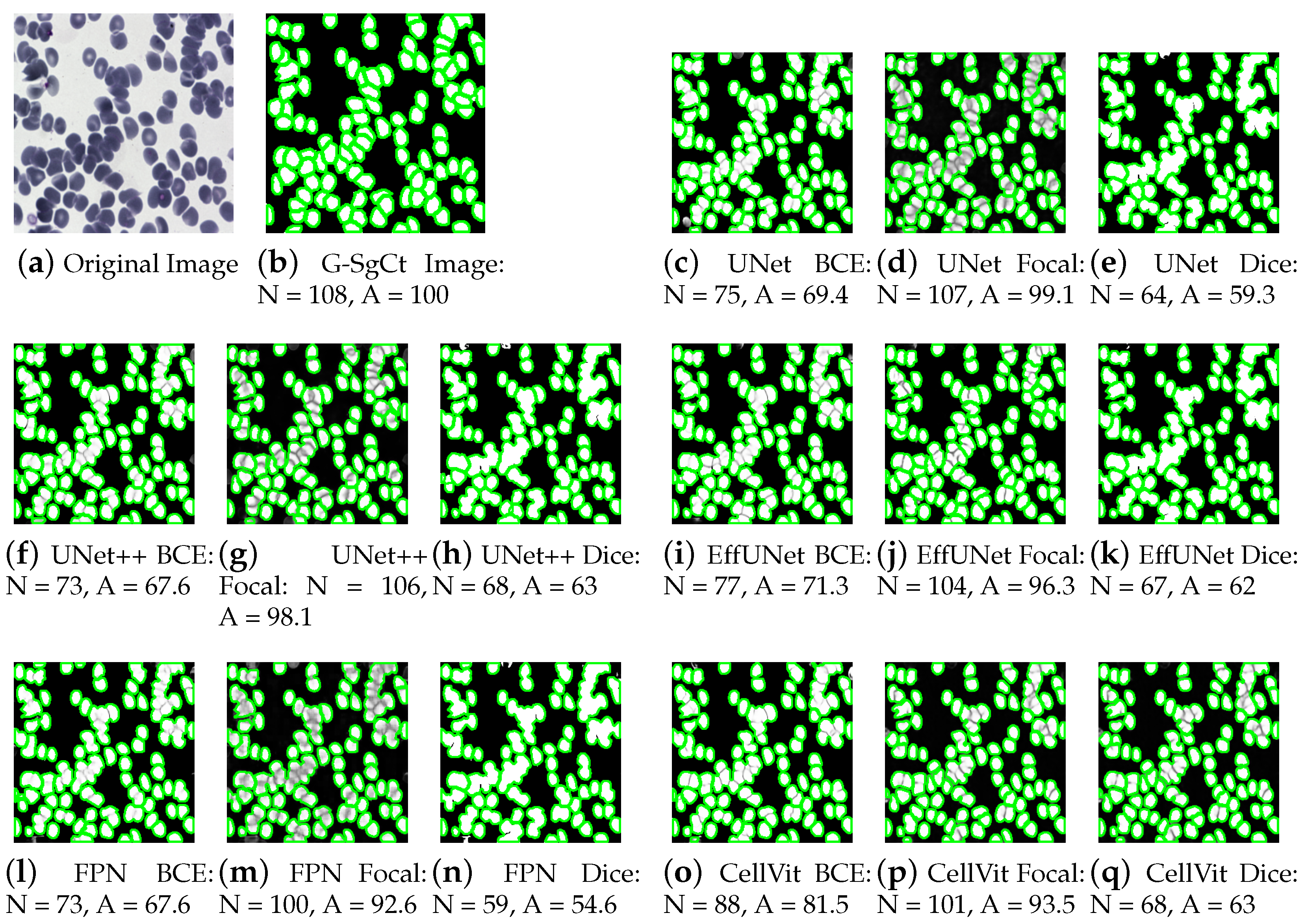
Figure 2 and Figure 3 illustrate representative examples of cell segmentation and counting results for both sparse and dense cell distributions. In sparse distributions, most model–loss combinations maintain stable cell counting accuracy above 92%, whereas in dense distributions the accuracy degrades to approximately 60% due to severe cell overlap and ambiguous boundaries. In the visualization, white regions indicate confidently segmented cell interiors, black regions correspond to non-cell background, and gray regions represent ambiguous transition areas between cell and non-cell regions. Although these gray areas may appear visually connected to cell contours, they are not interpreted as definitive cell boundaries unless they form sufficiently strong gradients in the distance transform. As a result, some visually merged contours in dense regions do not generate independent seed points, leading to an apparent mismatch between the number of visible contours and the final cell count N. Notably, compared to the baseline CellViT model trained with Dice loss, the proposed focal loss-based UNet++ improves counting accuracy by up to 55.7% in dense distributions, while the focal loss-based FPN achieves an improvement of up to 47%. This improvement indicates that the proposed CSC pipeline—through optimized segmentation model selection, loss function design, and adaptive watershed thresholding—produces smoother and more discriminative distance-transform gradients, enabling more reliable seed generation and boundary separation even in challenging dense-cell scenarios.

4.3. Performance Analysis of Model Compression

Table 3 compares cell counting accuracy (Acc), model size, and latency across three compression techniques: no quantization (baseline), FP16 quantization, and structured pruning. All results are measured on the same dataset under identical threshold conditions. For structured pruning, a consistent pruning ratio of 30% was applied across all architectures, followed by fine-tuning for 20 epochs to recover performance. This uniform pruning and retraining protocol ensures fair comparison among models and helps explain the observed differences in pruning sensitivity across network architectures.
Overall, FP16 Quantization provides the best efficiency without accuracy degradation, maintaining a balance between model size and inference speed. Compared to the FP32 baseline, FP16 reduces memory usage by approximately 50% and latency by 10–15%, while keeping accuracy loss below 1%. For example, UNet++ maintains 95% accuracy after FP16 quantization, while its model size decreases from 138.8 MB to 67.0 MB. Similarly, FPN and ResUNet preserve accuracies of 92% and 91%, respectively, with latency variations under 1 ms.
Conversely, structured pruning achieves substantial size reduction but introduces larger accuracy degradation in some models. BiFPN and EffUNet exhibit 3–4% accuracy loss as pruning intensity increases, likely due to the removal of critical skip-path connections between encoder and decoder layers. Furthermore, pruning occasionally increases latency slightly, despite model sparsity, due to unbalanced memory access patterns and non-uniform sparsity. For example, UNet latency rises modestly from 21.6 ms to 25.5 ms after pruning.
In terms of model trends, UNet++, UNet, and FPN demonstrate the best overall trade-offs under FP16 Quantization, maintaining stable counting accuracies of 95%, 93%, and 92%, respectively. Meanwhile, Transformer-based models such as CellViT and Evit-UNet show minor accuracy drops (92%→ 91%) due to the sensitivity of attention-weight scaling but negligible latency increases (1–2 ms).
In summary, FP16 Quantization is the optimal compression strategy, improving efficiency without sacrificing precision. Although Structured Pruning provides significant size reduction, it may negatively affect segmentation and counting performance. The best trade-off is achieved with FP16-Quantized UNet++, which delivers 95% accuracy, a 67 MB model size, and 29.5 ms latency. Thus, the proposed FP16-based lightweight counting pipeline is identified as the most efficient solution for low-power AIoT environments.

4.4. Cross-Dataset Validation on CHO Cell Images

In the previous sections, the proposed end-to-end CSC framework was extensively evaluated on the WBC dataset to analyze which segmentation models are most effective in terms of accuracy and computational efficiency, as well as which combinations of loss functions and watershed thresholds maximize cell counting performance. In this section, the same evaluation procedure is applied to a different cell domain, namely the Chinese Hamster Ovary (CHO) cell line dataset, in order to assess the generalization capability of the proposed approach. Specifically, segmentation performance across different models and loss functions, as well as cell counting accuracy under varying watershed thresholds, are systematically analyzed.
As shown in Table 4, results on the CHO cell dataset exhibit trends consistent with those observed in Table 1 for the WBC dataset. Most segmentation models demonstrate stable performance across different training losses, with UNet++ achieving the highest accuracy, Dice coefficient, sensitivity, and mIoU among all evaluated architectures. Meanwhile, FPN and ResUNet again demonstrate the most favorable efficiency characteristics when considering model size and inference latency, confirming their suitability for resource-constrained deployment.
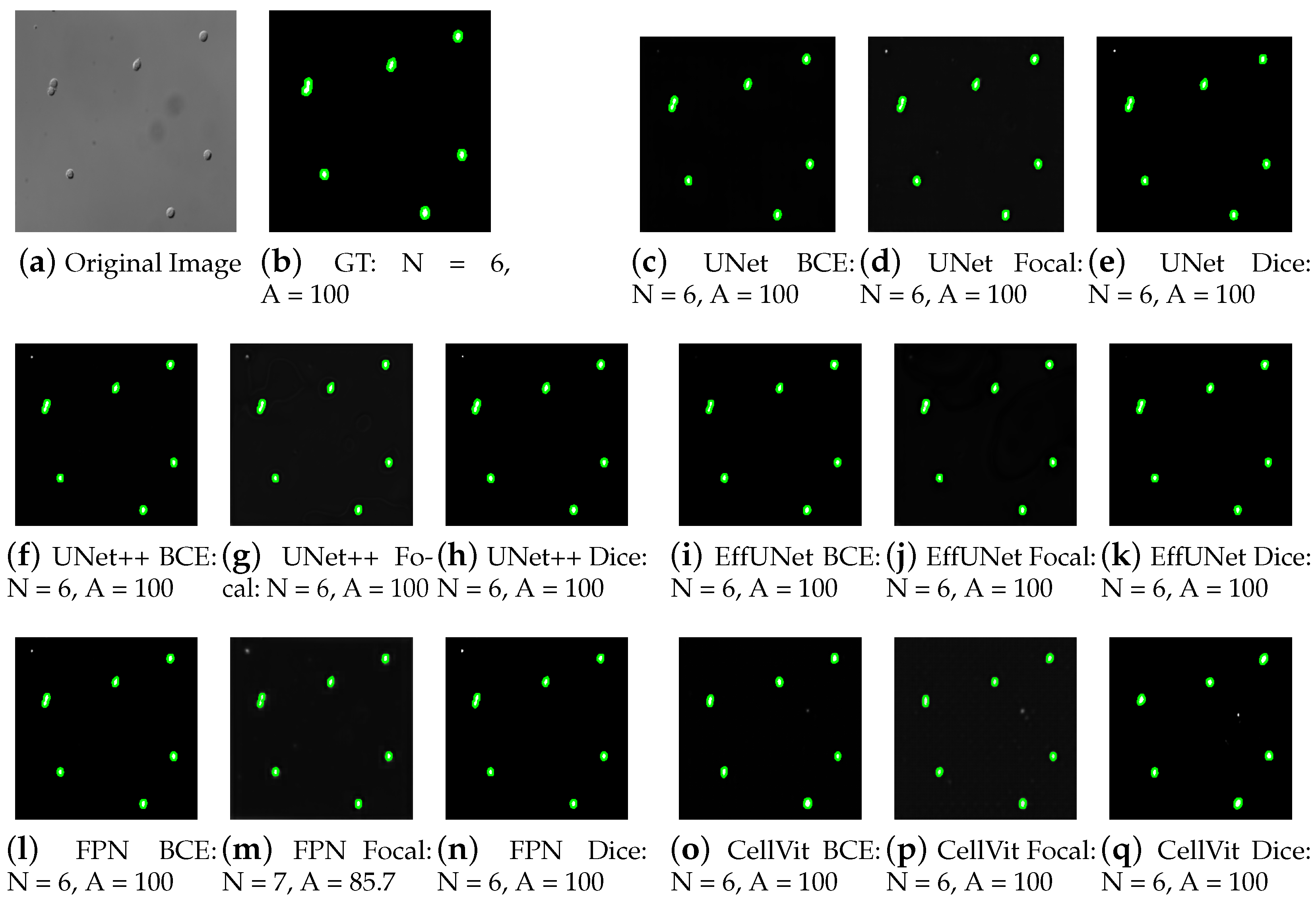
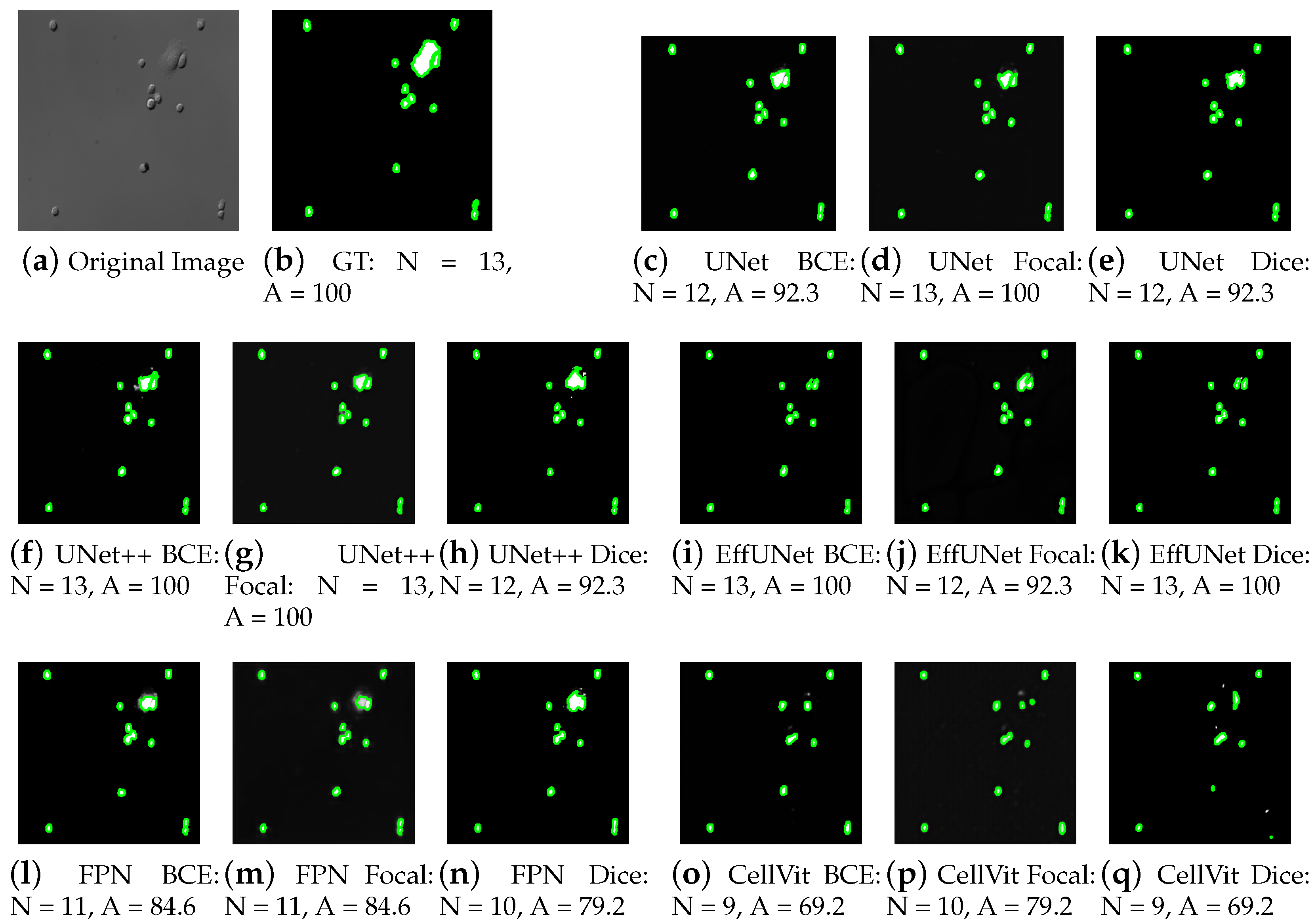
Table 5 presents the cell counting accuracy on the CHO cell dataset across different watershed threshold values. As illustrated in Figure 4 and Figure 5, the CHO cell images generally exhibit lower cell density compared to the WBC dataset. Consequently, robust counting performance is maintained over a wider range of watershed thresholds, indicating that the proposed CSC pipeline remains stable under less crowded cellular conditions.

5. Conclusions

This study presented an optimized end-to-end cell segmentation and counting (CSC) pipeline for low-power AIoT devices by jointly considering segmentation model selection, watershed-based counting optimization, and model compression. Experimental results demonstrate that a Focal-Loss-based FPN model with a watershed threshold of T w = 0.65 achieves the best overall counting performance. With FP16 quantization and pruning, the proposed pipeline improves cell counting accuracy by 21.1%, while reducing model size by 74.5% and inference latency by 16.8% compared to the baseline. These results confirm the effectiveness of the proposed framework as a lightweight and accurate CSC solution suitable for real-time AIoT deployment.

Author Contributions

Conceptualization, S.L.; methodology, S.L.; software, G.P., J.P. and S.L.; validation, S.L.; formal analysis, S.L.; investigation, S.L.; resources, S.L.; data curation, S.L.; writing—original draft preparation, S.L.; writing—review and editing, S.L.; visualization, S.L.; supervision, S.L.; project administration, S.L.; funding acquisition, S.L. All authors have read and agreed to the published version of the manuscript.

Funding

This work was supported by the Korea Evaluation Institute of Industrial Technology (KEIT) grant funded by the Korea government (MOTIE) (No. RS-2025-02313838, Project Name: Development of AI Training, Internalization, and Prediction System Technology for High-Speed, Multiplex, and Ultra-Precision Detection Based on Bio-Semiconductors).

Institutional Review Board Statement

Not applicable.

Informed Consent Statement

Not applicable.

Data Availability Statement

The original contributions presented in the study are included in the article, further inquiries can be directed to the corresponding author.

Conflicts of Interest

The authors declare no conflict of interest.

References

  1. Kobara, Y.M.; Akpan, I.J.; Nam, A.D.; AlMukthar, F.H.; Peter, M. Artificial intelligence and data science methods for automatic detection of white blood cells in images. J. Imaging Inform. Med. 2025. [Google Scholar] [CrossRef]
  2. Naouali, S.; Othmani, O.E. AI-driven automated blood cell anomaly detection: Enhancing diagnostics and telehealth in hematology. J. Imaging 2025, 11, 157. [Google Scholar] [PubMed]
  3. Abozeid, A.; Alrashdi, I.; Krushnasamy, V.S.; Gudla, C.; Ulmas, Z.; Nimma, D.; El-Ebiary, Y.A.B.; Abdulhadi, R. White blood cells detection using deep learning in healthcare applications. Alex. Eng. J. 2025, 124, 135–146. [Google Scholar] [CrossRef]
  4. Rezatofighi, S.; Soltanian-Zadeh, H. Automatic recognition of five types of white blood cells in peripheral blood. Cytom. Part A 2011, 79A, 747–757. [Google Scholar] [CrossRef]
  5. Nimmy, T.; Sreejith, V. A Review on White Blood Cells Segmentation. In Proceedings of the International Conference on Recent Advancements and Effectual Researches in Engineering Science and Technology (RAEREST), Kerala State, India, 20–21 April 2018. [Google Scholar] [CrossRef]
  6. Mohamed, A.; Farag, M.; Ghazal, H. Automatic white blood cell segmentation using deep learning. IEEE Access 2019, 7, 180449–180458. [Google Scholar]
  7. Xu, J.; Luo, F.; Li, S. AI-assisted digital hematology for remote blood cell analysis. Front. Med. 2021, 8, 678913. [Google Scholar]
  8. Darling, H.E.; Wheeler, R.T.; Lakowicz, J.R. Quantitative analysis of leukocyte morphology and viability for drug toxicity testing. Biotechnol. Bioeng. 2021, 118, 2234–2246. [Google Scholar]
  9. Ronneberger, O.; Fischer, P.; Brox, T. U-Net: Convolutional networks for biomedical image segmentation. In Medical Image Computing and Computer-Assisted Intervention, Proceedings of the MICCAI 2015; Munich, Germany, 5–9 October 2015, Springer: Cham, Switzerland, 2015; pp. 234–241. [Google Scholar]
  10. Zhou, Z.; Siddiquee, M.M.R.; Tajbakhsh, N.; Liang, J. UNet++: A Nested U-Net Architecture for Medical Image Segmentation. arXiv 2018, arXiv:1807.10165. [Google Scholar]
  11. Diakogiannis, F.I.; Waldner, F.; Caccetta, P.; Wu, C. ResUNet-a: A deep learning framework for semantic segmentation of remotely sensed data. arXiv 2020, arXiv:1904.00592. [Google Scholar] [CrossRef]
  12. Tan, M.; Le, Q.V. EfficientNet: Rethinking Model Scaling for Convolutional Neural Networks. arXiv 2019, arXiv:1905.11946. [Google Scholar]
  13. Lin, T.-Y.; Dollár, P.; Girshick, R.; He, K.; Hariharan, B.; Belongie, S. Feature Pyramid Networks for Object Detection. arXiv 2019, arXiv:1612.03144. [Google Scholar]
  14. Tan, M.; Pang, R.; Le, Q.V. EfficientDet: Scalable and Efficient Object Detection. In Proceedings of the IEEE/CVF Conference on Computer Vision and Pattern Recognition (CVPR 2020), Seattle, WA, USA, 13–19 June 2020. [Google Scholar]
  15. Kirillov, A.; Girshick, R.; He, K.; Dollár, P. Panoptic Feature Pyramid Networks. arXiv 2019, arXiv:1901.02446. [Google Scholar] [CrossRef]
  16. Dosovitskiy, A.; Beyer, L.; Kolesnikov, A.; Weissenborn, D.; Zhai, X.; Unterthiner, T.; Dehghani, M.; Minderer, M.; Heigold, G.; Gelly, S.; et al. An image is worth 16 × 16 words: Transformers for image recognition at scale. arXiv 2020, arXiv:2010.11929. [Google Scholar]
  17. Hörst, F.; Rempe, M.; Heine, L.; Seibold, C.; Keyl, J.; Baldini, G.; Ugurel, S.; Siveke, J.; Grünwald, B.; Egger, J.; et al. CellViT: Vision Transformers for Precise Cell Segmentation and Classification. arXiv 2023, arXiv:2306.15350. [Google Scholar] [CrossRef]
  18. Li, X.; Zhu, W.; Dong, X.; Dumitrascu, O.M.; Wang, Y. EViT-Unet: U-Net Like Efficient Vision Transformer for Medical Image Segmentation on Mobile and Edge Devices. arXiv 2023, arXiv:2410.15036. [Google Scholar]
  19. Khan, A.R.; Khan, A. Multi-axis vision transformer for medical image segmentation. Eng. Appl. Artif. Intell. 2025, 158, 111251. [Google Scholar] [CrossRef]
  20. Depto, D.S.; Rahman, S.; Hosen, M.M.; Akter, M.S.; Reme, T.R.; Rahman, A.; Zunair, H.; Rahman, M.S.; Mahdy, M.R.C. Automatic segmentation of blood cells from microscopic slides: A comparative analysis. Tissue Cell 2021, 73, 101653. [Google Scholar] [CrossRef]
  21. Sheikh, I.M.; Chachoo, M.A. A hybrid cell image segmentation method based on the multilevel improvement of data. Tissue Cell 2023, 84, 102169. [Google Scholar] [CrossRef]
  22. He, K.; Gkioxari, G.; Dollar, P.; Girshick, R. Mask R-CNN. In Proceedings of the IEEE International Conference on Computer Vision (ICCV), Venice, Italy, 22–29 October 2017; pp. 2961–2969. [Google Scholar]
  23. Graham, S.; Vu, Q.D.; Raza, S.E.A.; Azam, A.; Tsang, Y.W.; Kwak, J.T.; Rajpoot, N. Hover-Net: Simultaneous segmentation and classification of nuclei in multi-tissue histology images. Med. Image Anal. 2019, 58, 101563. [Google Scholar] [CrossRef] [PubMed]
  24. Adnan, N.; Umer, F.; Malik, S. Implementation of transfer learning for the segmentation of human mesenchymal stem cells—A validation study. Tissue Cell 2023, 83, 102149. [Google Scholar] [CrossRef]
  25. Hoorali, F.; Khosravi, H.; Moradi, B. Automatic microscopic diagnosis of diseases using an improved UNet++ architecture. Tissue Cell 2022, 76, 101816. [Google Scholar] [CrossRef]
  26. Blood Cell Segmentation Dataset. Available online: https://www.kaggle.com/datasets/jeetblahiri/bccd-dataset-with-mask (accessed on 26 December 2025).
  27. Chinese Hamster Ovary Cells. Available online: https://bbbc.broadinstitute.org/BBBC030?utm_source=chatgpt.com (accessed on 26 December 2025).
  28. Lempitsky, V.; Zisserman, A. Learning to Count Objects in Images. Adv. Neural Inf. Process. Syst. 2010, 23. [Google Scholar]
  29. Li, Y.; Zhang, X.; Chen, D. CSRNet: Dilated Convolutional Neural Networks for Understanding the Highly Congested Scenes. In Proceedings of the CVPR 2018, Salt Lake City, UT, USA, 18–22 June 2018. [Google Scholar]
  30. Xie, H.; He, Y.; Xu, D.; Kuo, J.Y.; Lei, H.; Lei, B. Joint segmentation and classification task via adversarial network: Application to HEp-2 cell images. Appl. Soft Comput. 2022, 114, 108156. [Google Scholar] [CrossRef]
  31. Archit, A.; Freckmann, L.; Nair, S.; Khalid, N.; Hilt, P.; Rajashekar, V.; Freitag, M.; Teuber, C.; Spitzner, M.; Contreras, C.T.; et al. Segment Anything for Microscopy. Nat. Methods 2025, 22, 579–591. [Google Scholar] [CrossRef] [PubMed]
  32. Wolf, S.; Lalit, M.; McDole, K.; Funke, J. Unsupervised Learning of Object-Centric Embeddings for Cell Instance Segmentation in Microscopy Images. In Proceedings of the 2023 IEEE/CVF International Conference on Computer Vision (ICCV), Paris, France, 2–6 October 2023; pp. 21206–21215. [Google Scholar]
  33. Israel, U.; Marks, M.; Dilip, R.; Li, Q.; Yu, C.; Laubscher, E.; Iqbal, A.; Pradhan, E.; Ates, A.; Abt, M.; et al. CellSAM: A foundation model for cell segmentation. Nat. Methods 2025, 22, 2585–2593. [Google Scholar] [CrossRef] [PubMed]
  34. Lee, H.; Lee, N.; Lee, S. A Method of Deep Learning Model Optimization for Image Classification on Edge Device. Sensors 2022, 22, 7344. [Google Scholar] [CrossRef] [PubMed]
  35. Hinton, G.; Vinyals, O.; Dean, J. Distilling the Knowledge in a Neural Network. In Proceedings of the NIPS 2014 Deep Learning Workshop, Montreal, QC, Canada, 12–13 December 2014. [Google Scholar]
  36. Elsken, T.; Metzen, J.H.; Hutter, F. Neural Architecture Search: A Survey. arXiv 2018, arXiv:1808.05377. [Google Scholar]
  37. Huang, G.; Liu, Z.; Maaten, L.v.; Weinberger, K.Q. Densely Connected Convolutional Networks. arXiv 2018, arXiv:1608.06993. [Google Scholar]
  38. Bishop, C.M.; Nasrabadi, N.M. Pattern Recognition and Machine Learning; Springer: New York, NY, USA, 2006. [Google Scholar]
  39. Dice, L.R. Measures of the Amount of Ecologic Association Between Species. Ecology 1945, 26, 297–302. [Google Scholar] [CrossRef]
  40. Lin, T.Y.; Goyal, P.; Girshick, R.; He, K.; Dollár, P. Focal Loss for Dense Object Detection. In Proceedings of the IEEE International Conference on Computer Vision, Venice, Italy, 22–29 October 2017; pp. 2980–2988. [Google Scholar]
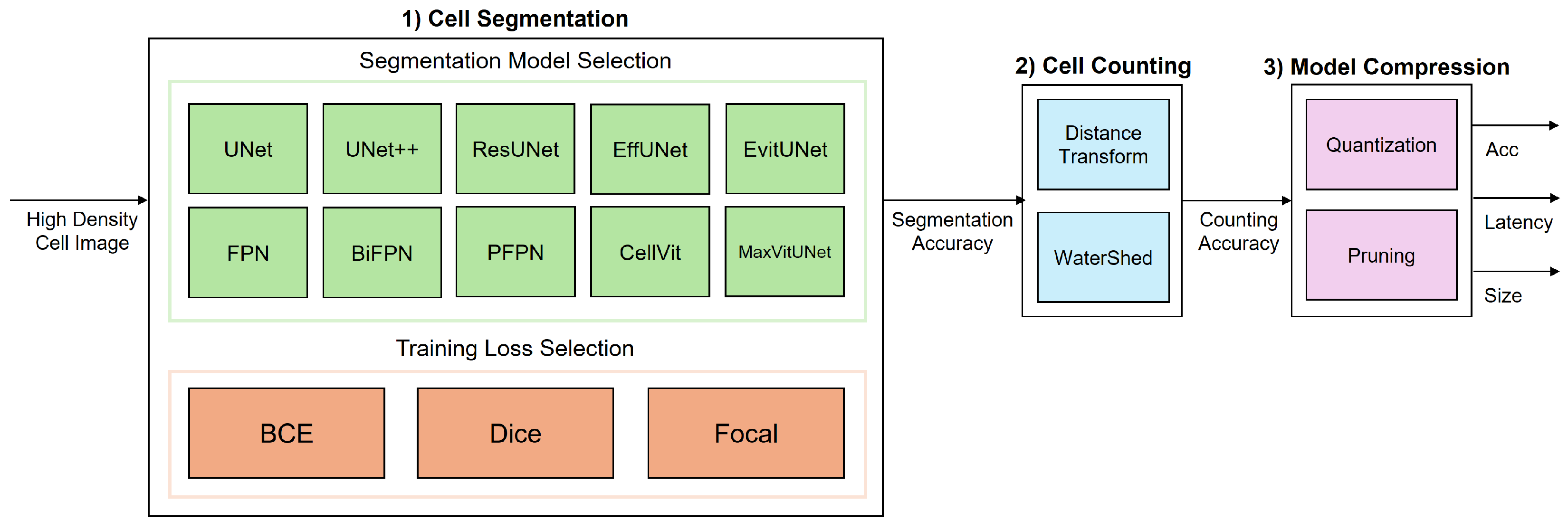
Figure 1. E2E pipeline optimization of cell segmentation and counting for low-power AIoT devices: The E2E pipeline optimization is performed by jointly considering cell segmentation, cell counting, and model compression.
Applsci 16 00357 g001
Figure 2. Result images of segmentation and counting in sparse cell distribution: GT denotes the ground truth annotation, N represents the total number of counted cells, and A indicates the cell counting accuracy. The green contours correspond to the segmented cell boundaries obtained by each segmentation model. Each sub-figure illustrates the cell segmentation and counting results produced by a specific combination of segmentation model and training loss, where the optimal watershed threshold is selected individually for each configuration.
Applsci 16 00357 g002
Figure 3. Result images of cell segmentation and counting in dense cell distribution: GT denotes the ground truth annotation, N represents the total number of counted cells, and A indicates the cell Counting accuracy. The green contours indicate the predicted cell boundaries generated by each segmentation model. Each sub-figure presents representative examples of cell segmentation and counting results using the optimal watershed threshold selected for each segmentation model and training loss combination under dense cell distribution conditions.
Applsci 16 00357 g003
Figure 4. Result images of segmentation and counting in sparse cell distribution: GT denotes the ground truth annotation, N represents the total number of counted cells, and A indicates the cell counting accuracy. The green contours indicate the predicted cell boundaries generated by each segmentation model. Each subfigure presents representative examples of cell segmentation and counting results using the optimal watershed threshold selected for each segmentation model and training loss combination under dense cell distribution conditions.
Applsci 16 00357 g004
Figure 5. Result images of cell segmentation and counting in dense cell distribution: GT denotes the ground truth annotation, N represents the total number of counted cells, and A indicates the cell counting accuracy. The green contours indicate the predicted cell boundaries generated by each Segmentation model. Each subfigure presents representative examples of cell segmentation and counting results using the optimal watershed threshold selected for each segmentation model and training loss combination under dense cell distribution conditions.
Applsci 16 00357 g005
Table 1. Cell segmentation results for blood cell segmentation dataset.
BCE LossFocal Loss
ModelAccDiceSensmIoUAccDiceSensmIoU
UNet98.096.596.893.497.996.396.493.0
UNet++98.096.597.293.497.996.496.293.2
ResUNet98.096.597.393.297.896.295.392.8
EffUNet97.896.396.992.997.796.095.992.4
FPN97.996.496.993.197.996.396.293.0
BiFPN97.495.696.391.597.996.396.293.0
PFPN97.996.496.593.197.996.396.293.0
CellVit97.295.295.690.896.994.793.989.9
EvitUNet97.896.196.892.597.495.594.691.5
MaxViTUNet97.996.496.793.097.896.196.092.6
Dice LossEfficiency
ModelAccDiceSensmIoUsize (MB)latency (ms)
UNet98.096.697.193.4124.321.6
UNet++98.096.597.193.3138.828.9
ResUNet98.096.597.393.326.921.5
EffUNet97.996.497.093.169.846.4
FPN98.096.597.193.216.721.5
BiFPN97.495.696.391.732.456.3
PFPN98.096.596.893.347.527.2
CellVit97.295.395.891.033.527.3
EvitUNet97.696.097.092.368.426.5
MaxViTUNet97.996.496.993.1133.542.7
Table 2. Cell counting accuracy according to threshold for the WBC dataset [26].
BCE LossThreshold
Model0.450.500.550.600.650.70.750.80.850.9
UNet0.810.820.830.840.860.880.890.910.910.92
UNet++0.800.810.820.830.810.810.890.900.910.91
ResUNet0.790.790.800.810.820.840.860.870.890.90
EffUNet0.840.870.890.900.910.910.910.920.920.92
FPN0.810.820.830.840.860.870.880.900.910.92
BiFPN0.780.790.800.820.840.860.880.900.910.91
PFPN0.790.810.820.830.850.870.890.910.910.92
CellVit0.780.790.810.820.840.850.870.880.890.90
EvitUNet0.790.800.820.840.850.870.890.910.920.92
MaxViTUNet0.840.860.880.910.930.940.950.950.950.96
Focal Loss
Model0.450.500.550.600.650.70.750.80.850.9
UNet0.860.910.920.930.920.920.920.910.890.85
UNet++0.900.940.950.950.950.930.930.920.900.89
ResUNet0.850.870.900.900.910.910.910.900.890.84
EffUNet0.890.910.910.910.910.910.910.910.910.91
FPN0.820.860.900.910.920.910.900.880.850.75
BiFPN0.840.890.910.910.910.910.910.910.910.89
PFPN0.840.890.920.920.920.920.920.900.870.82
CellVit0.830.880.900.910.920.910.910.890.870.80
EvitUNet0.900.920.920.920.920.920.910.910.910.91
MaxViTUNet0.930.950.950.950.950.960.960.960.960.96
Dice Loss
Model0.450.500.550.600.650.70.750.80.850.9
UNet0.800.800.800.800.800.800.800.800.800.81
UNet++0.810.810.810.810.850.870.810.810.810.81
ResUNet0.790.790.790.790.790.790.790.790.790.79
EffUNet0.890.910.910.910.910.910.910.910.910.91
FPN0.800.800.800.800.800.800.800.800.800.80
BiFPN0.760.760.760.760.760.760.760.760.760.76
PFPN0.800.800.800.810.810.810.810.810.810.82
CellVit0.760.760.760.770.770.770.770.770.780.78
EvitUNet0.810.810.810.810.820.820.820.820.820.82
MaxViTUNet0.820.820.820.820.820.820.830.830.830.83
Table 3. Cell counting accuracy according to model compression techniques.
ModelNo QuantizationFP16 QuantizationPruning
AccSizeLatencyAccSizeLatencyAccSizeLatency
UNet93124.321.69362.223.69179.425.5
UNet++95138.828.99567.029.59385.431.2
ResUNet9126.921.59113.421.48817.122.7
FPN9216.721.1928.422.78913.223.1
BiFPN9132.441.39116.436.18727.243.4
PFPN9247.527.29223.824.38830.220.4
EffUNet9169.826.49235.029.88744.825.1
CellVit9233.527.39116.828.48928.129.3
EvitUNet9268.426.59134.226.98842.731.2
MaxViTUNet96133.544.99663.844.057117.2850.6
Table 4. Cell segmentation results for CHO cell segmentation dataset [27].
BCE LossFocal Loss
ModelAccDiceSensmIoUAccDiceSensmIoU
UNet99.791.992.985.399.792.291.685.7
UNet++99.793.193.887.399.792.592.586.3
ResUNet99.792.592.286.399.792.090.085.5
EffUNet99.586.081.675.999.483.875.172.7
FPN99.792.393.885.999.691.089.683.8
BiFPN99.381.980.969.699.379.674.366.6
PFPN99.791.791.884.999.791.390.984.3
CellVit99.278.676.365.599.277.469.763.9
EvitUNet99.792.091.985.499.690.789.483.3
MaxViTUNet99.791.592.084.599.691.191.584.0
Dice LossEfficiency
ModelAccDiceSensmIoUsize (MB)latency (ms)
UNet99.792.892.786.7124.311.28
UNet++99.793.295.087.3138.817.04
ResUNet99.792.893.286.826.911.33
EffUNet99.588.084.379.169.819.35
FPN99.792.694.286.316.710.46
BiFPN99.380.578.667.832.432.09
PFPN99.792.893.286.847.511.41
CellVit99.073.269.658.433.520.72
EvitUNet99.691.091.583.868.413.34
MaxViTUNet99.792.092.385.4133.531.52
Table 5. Cell counting accuracy according to threshold for the CHO dataset dataset [27].
BCE LossThreshold
Model0.450.500.550.600.650.70.750.80.850.9
UNet0.940.940.950.950.950.950.950.950.950.95
UNet++0.960.960.950.950.940.940.950.950.950.96
ResUNet0.950.940.940.940.930.940.920.920.930.91
EffUNet0.950.940.940.940.950.950.950.950.950.96
FPN0.940.940.940.940.950.950.940.950.950.95
BiFPN0.950.950.940.940.940.930.920.920.910.91
PFPN0.950.950.950.950.950.950.950.950.960.97
CellVit0.920.920.920.920.920.910.910.910.910.91
EvitUNet0.950.950.940.940.940.960.960.960.940.94
MaxViTUNet0.960.960.960.960.960.960.960.960.960.96
Focal Loss
Model0.450.500.550.600.650.70.750.80.850.9
UNet0.950.950.960.950.950.950.950.960.960.95
UNet++0.950.960.960.960.950.950.950.950.960.96
ResUNet0.950.940.940.940.930.940.920.920.930.91
EffUNet0.960.940.940.950.950.950.960.960.950.93
FPN0.940.950.940.940.950.950.940.940.900.91
BiFPN0.950.940.930.940.940.940.950.920.920.89
PFPN0.960.960.960.960.960.960.950.960.970.97
CellVit0.910.900.900.910.910.910.910.910.900.90
EvitUNet0.950.960.950.950.960.950.950.940.950.93
MaxViTUNet0.940.940.940.950.950.950.950.950.970.97
Dice Loss
Model0.450.500.550.600.650.70.750.80.850.9
UNet0.960.960.960.960.960.960.960.960.960.96
UNet++0.960.960.960.960.960.960.960.960.960.96
ResUNet0.950.950.960.960.960.970.970.970.970.97
EffUNet0.950.950.950.950.950.950.950.950.950.95
FPN0.950.950.950.950.950.950.950.950.950.95
BiFPN0.930.930.920.920.920.920.930.930.940.94
PFPN0.960.960.960.970.970.970.970.970.970.97
CellVit0.880.880.880.880.880.880.880.880.880.88
EvitUNet0.950.950.950.950.950.950.950.950.950.95
MaxViTUNet0.950.940.940.940.940.940.940.940.940.95
Disclaimer/Publisher’s Note: The statements, opinions and data contained in all publications are solely those of the individual author(s) and contributor(s) and not of MDPI and/or the editor(s). MDPI and/or the editor(s) disclaim responsibility for any injury to people or property resulting from any ideas, methods, instructions or products referred to in the content.