Bayesian Poisson Modeling of Built Environment Effects on Pedestrian Crash Risk Among Older Adults in Mountainous Urban Areas

Abstract

In the context of rapid population aging in China, ensuring pedestrian safety for older adults has become a critical concern, particularly in mountainous cities where the built environment’s role remains understudied. This study examines how built environment factors influence road traffic crashes involving older pedestrians in such terrains, aiming to propose targeted safety optimization strategies. Using ten-year road traffic crash data from Yuzhong District, Chongqing, the research employed both Standard Poisson Regression and Bayesian Poisson Regression models for analysis. Key findings indicate that crash frequency significantly increased with higher densities of footbridges and recreational facilities, as well as with a greater proportion of parks and green space, whereas it decreased with a higher land use mix, greater densities of educational facilities, and higher public transport stop density. The proportion of storage land and the density of medical facilities showed no significant effects. These results provide concrete, evidence-based guidance for urban planning and transportation management in mountainous cities to optimize pedestrian infrastructure and enhance walking safety for the elderly.

1. Introduction

The most significant trend in global demographic change is population aging [1]. As the world’s second-most populous developing nation, China is experiencing increasingly prominent aging trends. The proportion of residents aged 65 and above rose from 8.9% (118.94 million) in 2010 to 15.6% (220.23 million) in 2024. China has one of the highest injury-related mortality rates among older adults globally. The leading causes of injury-related deaths are falls, traffic accidents, and suicide, with traffic accidents ranking as the second-most prevalent cause [2]. Walking serves as the primary mode of transportation for older adults, facilitating both daily activities [3] and environmental engagement [4]. However, age-related declines in physical and cognitive functions progressively impair their ability to perceive traffic environments and assess potential hazards. These physiological changes result in slower response times to sudden dangers [5,6]. Consequently, older pedestrians face significantly higher risks of severe injury and mortality in traffic incidents compared to other age groups [7].

Urban planners are increasingly recognizing the critical need to enhance pedestrian safety. In China, the rapid growth of the older adult population has brought heightened attention to the safety of older pedestrians. From 2016 to 2020, traffic incidents involving older adults increased by 163.2% on average compared to the 2011–2015 period, with annual fatalities and injuries rising by 62.5% and 74.3%, respectively. These traffic incidents can be attributed to multiple factors: driver-related causes [8], age-related declines in older pedestrians’ physical and cognitive abilities [6], and behavioral factors such as non-compliance with traffic rules and distraction behaviors (e.g., electronic device usage or roadside conversations) [9,10,11]. In addition, an age-unfriendly built environment may exacerbate safety risks for older pedestrians [12,13,14]. Despite growing concerns about pedestrian safety in aging populations, current understanding remains limited regarding how built factors influence older-pedestrian accidents. Existing research on built environment-traffic accident relationships predominantly employs the “3Ds” (density, diversity, design) or “5Ds” (density, diversity, design, destination accessibility, distance to transit) frameworks, with limited consideration of mountainous urban contexts within these analytical structures. Given the topographical constraints of steep slopes, limited developable land, and acute traffic congestion characteristic of mountainous cities, extensive networks of pedestrian overpasses and underground passes have been constructed to alleviate surface-level traffic pressure. Prevailing studies have frequently neglected the safety implications of these vertical circulation infrastructures for aging pedestrians.

Regarding methodological approaches, prior research on older-pedestrian safety has predominantly employed negative binomial regression models [15], with primary emphasis on point estimation. While point estimates provide specific parameter values, they fail to quantify parameter uncertainty. Machine learning algorithms are increasingly utilized to capture complex nonlinear relationships between built environment characteristics and collision risks, but these models suffer from limited interpretability. This study adopts the Bayesian Poisson Regression approach, integrating observed data with prior distributions to derive posterior parameter distributions that explicitly account for data-driven uncertainty. Yuzhong District, as one of the primary urban cores of Chongqing, boasts complex terrain and unique built environment characteristics across dimensions including density, diversity, and design, making it an ideal case study for examining how multidimensional built environment factors influence the risk of older-pedestrian crashes.

This study first reviews current understanding of built environment impacts on older-pedestrian safety, highlighting limitations in conventional analysis methods. The subsequent Section 3 employs a Bayesian approach to address these gaps, with particular attention to uncertainty quantification. The empirical results identify statistically significant built environment risk factors, with subsequent discussion of their urban planning implications. The work concludes with specific recommendations for creating age-friendly pedestrian infrastructure.

2. Literature Review

2.1. Built Environment Factors Influencing Pedestrian Safety

Extensive research demonstrates that older pedestrians experience significantly higher injury vulnerability compared to pedestrians of other ages [16]. When older pedestrians encounter complex traffic situations, their characteristically cautious behavior creates challenges for drivers to accurately assess crossing intentions, particularly during street-crossing maneuvers [17]. Age-related cognitive declines impair older pedestrians’ hazard detection capabilities and compromise their implementation of safety measures, so they are more likely to expose themselves to hazardous traffic conditions [18].

Prior studies have identified multiple aspects of the built environment influencing pedestrian traffic accidents, such as land use diversity, urban design, and density. Scholars have found that land use mix exhibits positive or negative correlations with pedestrian crashes. Chen et al. found a positive association between land use mix and the probability of pedestrian–vehicle collisions—with higher land use mix corresponding to increased crash likelihood—reflecting an increase in conflict points in areas with high land use mix due to concentrated pedestrian activities [19]. In contrast, Wang et al. observed an inverse relationship, where greater land use mix was associated with reduced pedestrian crash incidence, indicating that mixed land use enhances safety by controlling pedestrian exposure and fostering a more active and alert pedestrian environment [20]. Additionally, land use types can affect pedestrian safety. Concentrated commercial land use tends to create pedestrian attraction hubs, thereby increasing vehicle–pedestrian conflicts [21,22]. However, when such concentration forms commercial districts or large shopping centers with stringent traffic control measures, the occurrence of traffic accidents may actually decrease due to enhanced safety regulations. Research findings demonstrate a negative correlation between residential land use and pedestrian safety, whereas the number of residential units shows a positive association with pedestrian travel safety [23]. Bus stop density and distribution patterns significantly affect pedestrian safety [20,24]. When buses are stationary at stops, they generate sightline blockages that compromise pedestrians’ ability to perceive roadway dangers during crossing maneuvers, resulting in increased safety risks [25]. However, some studies suggest that more transit stops can reduce vehicle-miles traveled per capita and thereby enhance pedestrian safety in neighborhoods [26]. In roadway design, crosswalks serve as a critical infrastructure element that promotes spatial balance between pedestrians and vehicles, regulates movement patterns, and reduces traffic speeds [27]. Furthermore, empirical studies demonstrate that signalized intersections positively impact pedestrian safety [28], as enhanced traffic control measures and increased driver vigilance at these locations collectively contribute to reduced accident rates.

Despite considerable research on the relationship between the built environment and pedestrian safety, studies addressing older-pedestrian safety remain limited. Older-pedestrian safety correlates significantly with the presence of hospitals, markets, stores, and banks—facilities central to seniors’ daily activities. These infrastructure elements may enhance drivers’ awareness of elevated pedestrian volumes, thereby creating traffic calming effects. Paradoxically, however, the same facilities may lead to increased exposure to traffic conflicts for older pedestrians, resulting in higher crash risks [6]. This is particularly critical in the context of educational facilities, which serve as major pedestrian congregation points during school pickup/drop-off periods—a prevalent scenario in China where grandparents are mainly responsible for the transportation of their grandchildren to school.

Chongqing’s mountainous terrain imposes severe spatial constraints, necessitating footbridges and underground passes to mitigate traffic congestion—particularly in dense urban areas like Yuzhong District. While these structures improve pedestrian–vehicle segregation, their safety implications remain understudied. Our study addresses this gap by explicitly incorporating pedestrian underground passes and footbridges as critical variables in analyzing determinants of senior pedestrian crashes in Chongqing.

2.2. Analysis Method for Pedestrian Accident

Studies on built environment–pedestrian accident relationships employ spatial analysis, statistical modeling, and machine learning methods. Da Silva Mariana Teixeira analyzed the spatial distribution of older pedestrians knocked down by vehicles in Maringá City from 2014 to 2018. Accident hotspots were identified using kernel density estimation, and a qualitative comparison was conducted to examine the relationship between the spatial relative risk of traffic accidents involving older adults and the built environment [28]. Zhang et al. integrated Bayesian hierarchical models to identify spatiotemporal high/low clustering patterns of traffic accidents [29].

The negative binomial regression model is the most widely used statistical method in this field. The frequency of pedestrian–vehicle crashes typically follows a non-negative integer distribution, which is fundamentally characterized by a Poisson process. Consequently, the Poisson Regression models were predominantly utilized in early-stage research to examine the relationship between built environment factors and pedestrian crash occurrences. Subsequently, to address the issue of overdispersion frequently observed in crash count data, the negative binomial regression model was introduced as an enhanced analytical approach [7]. Daniel Gálvez-Pérez conducted a comparative analysis of the impacts of built environment factors on traffic accidents involving older versus younger pedestrians in Madrid using a negative binomial regression model [15].

Emerging studies have begun using machine learning algorithms to capture the complex, nonlinear associations between built environment characteristics and crash risks [30]. However, machine learning models (e.g., neural networks, random forests, and XGBoost) typically operate as “black boxes” with opaque decision-making processes [31], making it difficult to intuitively interpret the directional effects or magnitude of individual built environment factors (e.g., road width, traffic signal density) on crash rates. Even when employing post hoc interpretation tools like SHAP values or feature importance scores, the derived conclusions may demonstrate instability or contradict established domain knowledge [32].

Bayesian Poisson Regression extends traditional Poisson Regression by incorporating prior knowledge with observed data through Bayesian inference, thereby enabling more robust parameter estimation, comprehensive uncertainty quantification, and improved predictive accuracy [33]. Some studies have demonstrated that Bayesian Poisson Regression yields better results than both least squares and ordinary Poisson Regression in analyzing the influencing factors of traffic accidents [34,35]. Compared to machine learning models, Bayesian Poisson Regression offers distinct advantages in statistical interpretability, uncertainty quantification, small-sample performance, and prior knowledge integration [33], whereas machine learning excels at automated feature engineering, high-dimensional data processing, and capturing nonlinear relationships.

This study therefore examines the effects of various built environments on older-pedestrian accidents by using Bayesian Poisson Regression. The findings are particularly important for mountainous cities to determine built environmental attributes to improve the safety of older pedestrians and cope with the aging society.

3. Methodology

3.1. Research Framework

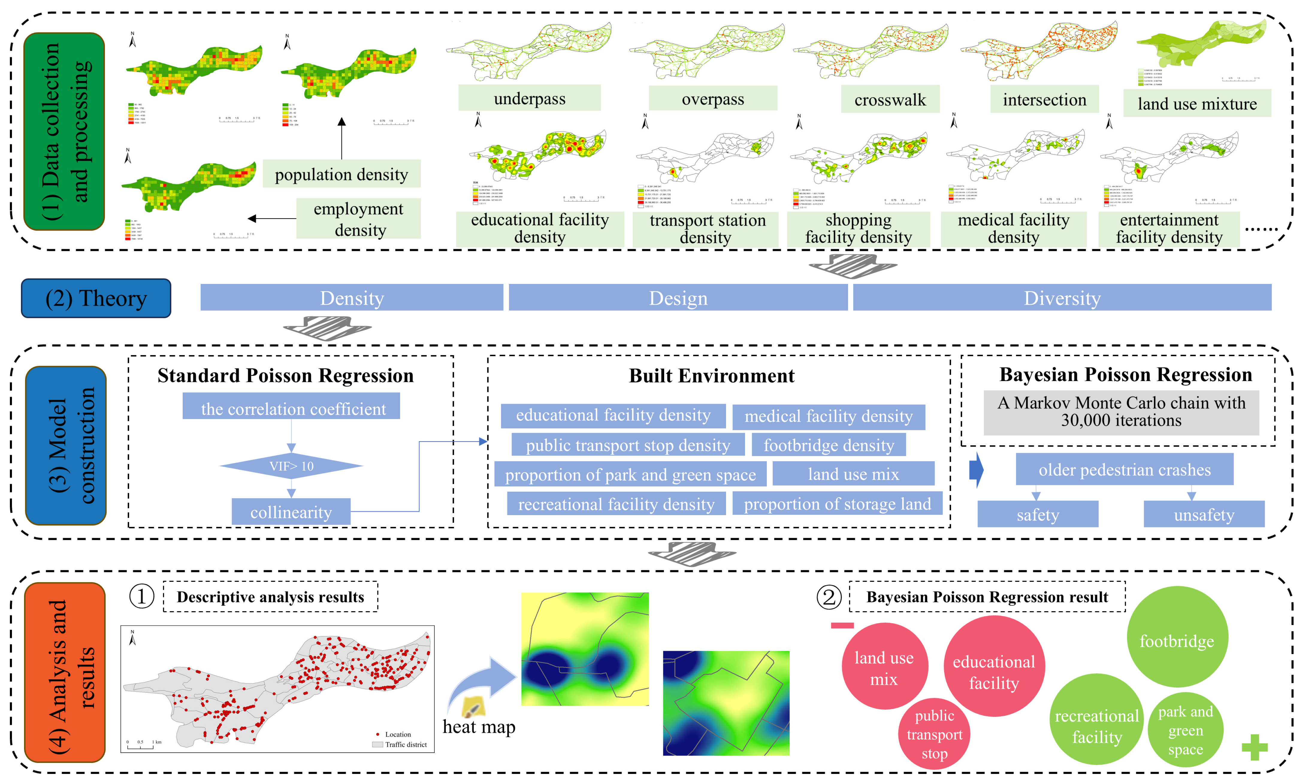
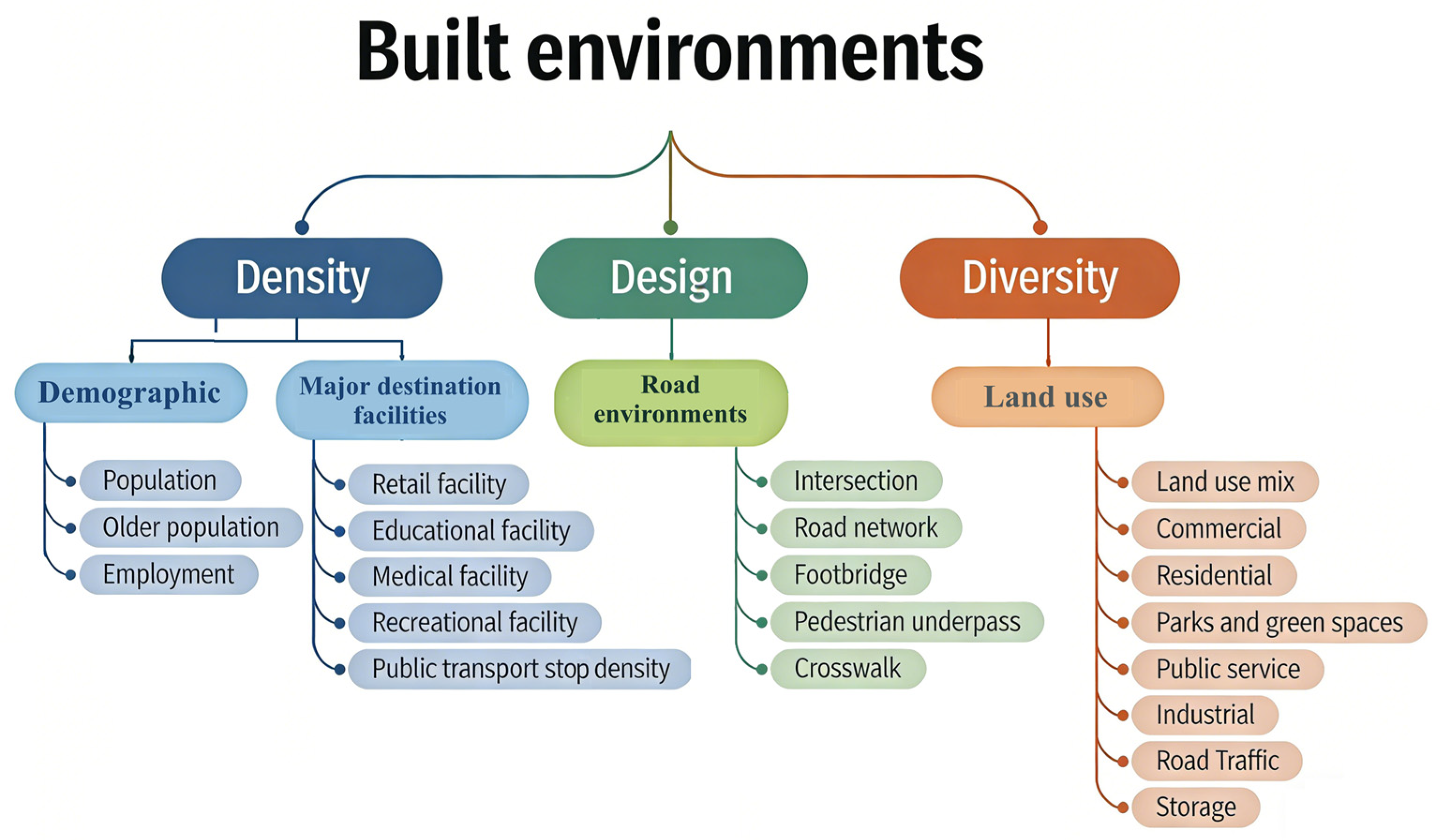
The conceptual framework of this study is illustrated in Figure 1. The independent variable set (X) consists of built environment variables, which were collected and reconstructed from multiple data sources based on the “3Ds” theoretical framework (density, design, and diversity) [36]. Among these independent variables, parameters representing pedestrian overpasses and underground passages—the most characteristic infrastructure elements in mountainous cities—have been incorporated. The target variable (Y) is the frequency of traffic accidents involving older adults, calculated from the traffic police patrol database within the study area and aggregated by traffic analysis zones.

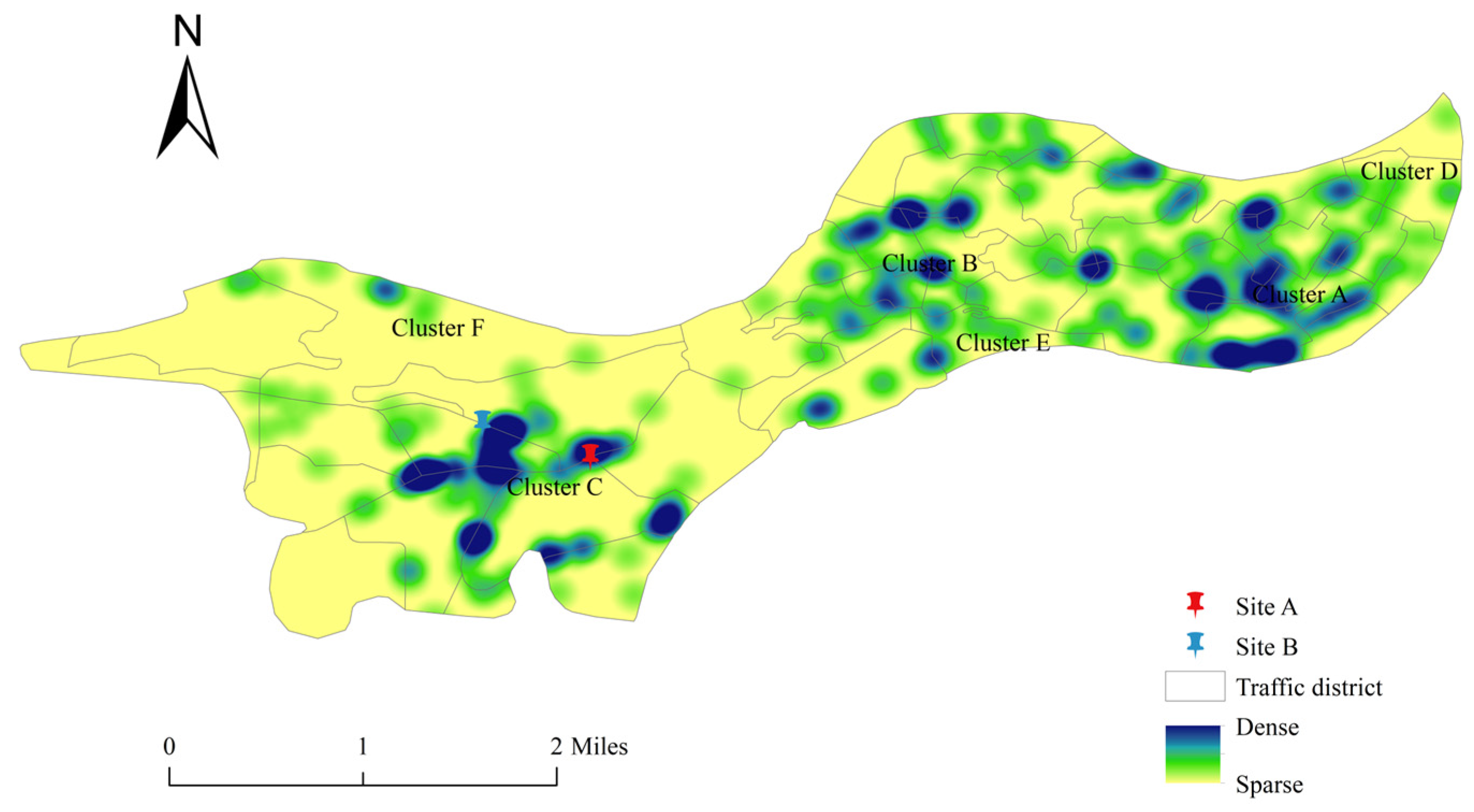
Methodologically, this study first eliminates collinearity among built environment factors through a correlation matrix screening process, then employs Standard Poisson Regression to identify statistically significant built environment variables, and subsequently utilizes Bayesian Poisson Regression to estimate both the direction (positive/negative) and magnitude of each built environment variable’s impact on pedestrian collision frequency. Additionally, kernel density estimation was applied to analyze the spatial clustering patterns of existing elderly traffic accidents, providing empirical support for localized traffic safety policy formulation.

3.2. Study Area

Our traffic data were collected within Yuzhong District in Chongqing, a megacity with a population of 30 million (Figure 2). According to the Seventh National Population Census of Chongqing, Yuzhong District has a permanent population of 588,717, of which 19.76% are aged 60 or above, and 14.03% are aged 65 or above. Chongqing has implemented a renovation and upgrading plan for older residential communities, integrating age-friendly and barrier-free environment improvements into urban renewal projects. Creating a senior-friendly built environment has become one of the most important policy priorities.

3.3. Data Sources

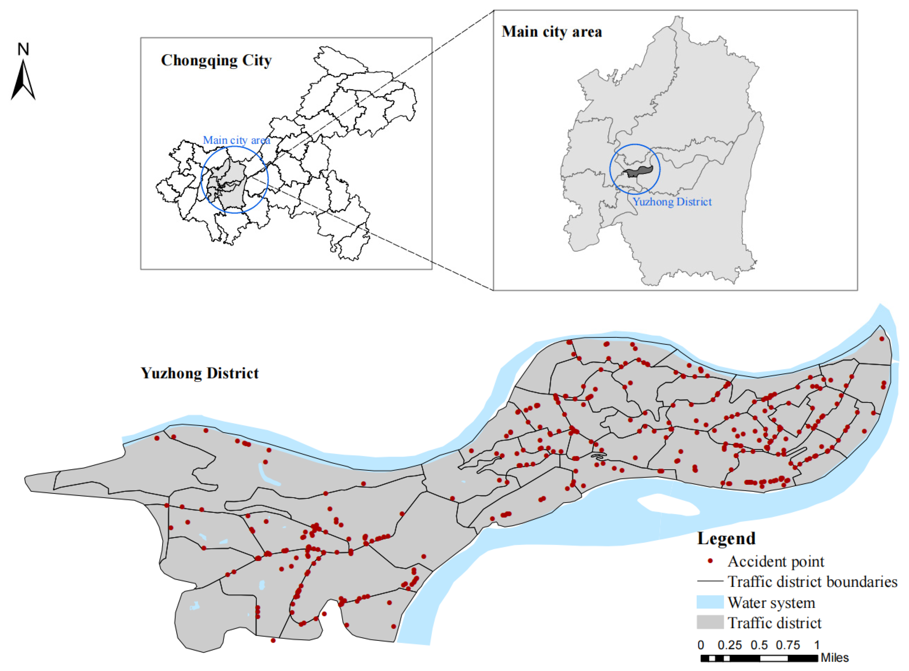
The traffic accident data of older pedestrians used in the study came from the traffic patrol police detachment of the study area, and we obtained a total of 2580 traffic accident data records in the study area from 2010 to 2021, including 854 walking accidents and 477 accidents involving older pedestrians. In the accident data, records involving two older pedestrians in the same accident were merged, and cases with unknown accident locations were excluded, resulting in a final dataset of 392 older-pedestrian crash records.

The demographic data were obtained from China Unicom’s mobile signaling data, with the dataset structured in 250 m × 250 m grid units for June 2021. This study calculated the monthly averages of both total population and older population for each grid within the study area. Employment population was defined as daytime-only population counts across all grids during the same one-month period. The mobile signaling data used in this research represent anonymized and expanded datasets of China Unicom users in the study area. While these processed data effectively preserve personal privacy by removing identifiable information, they maintain sufficient spatial resolution to reliably reflect population distribution patterns at the neighborhood scale. Subsequently, based on the vector maps of 50 traffic analysis zone (TAZ) boundaries, the constructed grids were spatially overlaid with TAZ boundaries using the spatial overlay analysis tool in ArcGIS 10.8 software, and the overlaid data were aggregated and calculated by TAZ affiliation, thereby yielding demographic data at the TAZ level.

The land use data was obtained by vectorizing remote sensing images using ArcGIS software. The remote sensing imagery consists of high-precision 2019 data for Yuzhong District, with a resolution of 2 m × 2 m, a spatial reference system of GCS_WGS_1984, and a datum of D_WGS_1984. The point of interest (POI) data was sourced from the Amap Open Platform (https://lbs.amap.com/ (accessed on 14 July 2024)), covering various categories in Yuzhong District, Chongqing, including shopping, entertainment, healthcare, and more. The dataset includes geographic locations (latitude and longitude coordinates) and facility types.

The road network data was obtained from the OpenStreetMap (OSM) database (https://www.openhistoricalmap.org/ (accessed on 17 July 2024)) and refined using ArcGIS software, incorporating both map references and field surveys. Additionally, data from roadside environmental facilities was collected through field survey.

3.4. Models

When the dependent variable follows a Poisson distribution, the Poisson Regression model is used; otherwise, a negative binomial model is used. This study conducted a distribution test on accident data of older pedestrians and found that it follows a Poisson distribution. For comparative purposes, the Standard Poisson Regression (SPR) model was also fitted as a baseline to evaluate the goodness-of-fit relative to the Bayesian approach.

3.4.1. Standard Poisson Regression (SPR)

Assuming that the number of older-pedestrian crashes, denoted as $Y_i$, in the i-th analysis zone follows a Poisson distribution with parameter ${\lambda }_i$, the probability density function of the crash frequency is as follows:

$$p\left(Y=y_i|x_i,E_i\right)={\displaystyle \raisebox{1ex}{$e^{-{\lambda }_i}{\lambda }_i^{y_i}$}\!\left/ \!\raisebox{-1ex}{$y_i$}\right.}!$$

(1)

$${\lambda }_i=E_i\mathrm{e}\mathrm{x}\mathrm{p} \left({\beta }^T{x}_i\right) (\mathrm{i}=1,2,3,\dots ,\mathrm{n})$$

(2)

where i is TAZ ID, Y_i is the number of older-pedestrian crashes, λ_i is the expected crash rate, x_i is the vector of independent variables, E_i is the total older population, and β_j is the regression coefficient.

By taking the logarithm of both sides of Equation (2), we obtain the following:

$$\log \left({\lambda }_i\right)={\beta }_0+\sum _{j=1}^p{\beta }_j{X}_{ij}+\log \left(E_i\right)$$

(3)

where $\log \left(E_i\right)$ is the exposure offset term, used to control the confounding effect of the older population base. The model ultimately predicts the crash rate per unit older population rather than the absolute count. All density-related variables (e.g., medical facility density, employment density) are built environment risk factors, not proxies for exposure. Only the total older population (target at-risk group) is selected as the exposure measure; the total population is not included since older pedestrians are the core research focus.

The maximum likelihood estimator (MLE) of parameter β can then be obtained from the following log-likelihood function:

$$\ln L\left(\beta \right)=\sum _{i=1}^N\left[y_i\log \left({\lambda }_i\right)-{\lambda }_i-\log \left(y_i!\right)\right]$$

(4)

Substituting ${\lambda }_i=E_i\mathrm{e}\mathrm{x}\mathrm{p} \left({\beta }^T{x}_i\right)$ into the equation, the log-likelihood function can be rewritten as follows:

$$\ln L\left(\beta \right)=\sum _{i=1}^N\left[y_i\left(\log \left(E_i\right)+{\beta }^T{x}_i\right)-E_i\mathrm{e}\mathrm{x}\mathrm{p}\left({\beta }^T{x}_i\right)-\log \left(y_i!\right)\right]$$

(5)

3.4.2. Bayesian Poisson Regression (BPR)

Bayesian Poisson Regression (BPR) adopts a framework where the likelihood function characterizes data patterns, the prior distribution incorporates parameter beliefs, and Markov Chain Monte Carlo (MCMC) sampling approximates the posterior distribution. It serves as a complement to the Maximum Likelihood Estimation (MLE) of Standard Poisson Regression (SPR), enabling the quantification of parameter uncertainty under small-sample conditions.

It is assumed that the regression coefficients follow weakly informative normal priors with different variances for intercept and slopes:

$${\beta }_0~\mathrm{N}\left(0,5^2\right), {\beta }_j~N\left(0,2^2\right), j= 1, 2, ..., p$$

(6)

where β₀ is the intercept term, β_j are the coefficients of independent variables, 5² is the prior variance of the intercept, and 2² is the prior variance of slopes.

The likelihood function of the Bayesian model is consistent with that of SPR. Thus, the logarithmic likelihood function is as follows:

$$\ln p\left(Y|\beta \right)=\sum _{\mathrm{i}=1}^{\mathrm{n}}\left\{\left(\log \left(E_i\right)+{\beta }^T{x}_i\right)-E_i\mathrm{e}\mathrm{x}\mathrm{p}\left({\beta }^T{x}_i\right)-\log \left(y_i!\right)\right\}$$

(7)

The joint distribution of the dataset Y and parameter β is the product of the likelihood function and the prior distribution. Further substituting the Standard Poisson Regression model into the above formula, we obtain the following:

$$\mathrm{p}\left(Y,\mathsf{\beta }\right)=\left[\prod _{\mathrm{i}=1}^{\mathrm{n}}{\displaystyle \frac{\mathrm{e}\mathrm{x}\mathrm{p}\left(-{\mathsf{\lambda }}_{\mathrm{i}}\right){\mathsf{\lambda }}_{\mathrm{i}}^{{\mathrm{y}}_{\mathrm{i}}}}{{\mathrm{y}}_{\mathrm{i}}!}}\right]·{\displaystyle \frac{1}{\sqrt{{\left(2\pi \right)}^n\left|{\sum }_{\beta }\right|}}}exp\left\{-{\displaystyle \frac{1}{2}}{\left(\beta -{\lambda }_{\beta }\right)}^T{\sum }_{ \beta }^{-1}\left(\beta -{\lambda }_{\beta }\right)\right\}$$

(8)

The posterior distribution is as follows:

$$\pi \left(\beta |Y\right)={\displaystyle \frac{p\left(Y,\beta \right)}{\int p\left(Y,\beta \right)d\beta }}$$

(9)

The posteriori expectation of parameter β is estimated as follows:

$$\widehat{\beta }=E\left(\beta |Y\right)=\int \beta p\left(\beta |Y\right)d\beta$$

(10)

The core assumption of Poisson likelihood is conditional equidispersion (mean ≈ variance given covariates), and weakly informative priors cannot address overdispersion in the likelihood function. Diagnostic tests confirmed substantial overdispersion in our data, with the dispersion ratio for the Standard Poisson Regression (SPR) being 6.22 (

Table 1. Model comparison results.

Model Type	AIC	BIC	Residual Deviance	Degrees of Freedom	Dispersion Ratio (Deviance/Degrees of Freedom)	Recommendation
Standard Poisson Regression	438.22	455.43	255.15	41	6.2232	Not recommended (due to overdispersion)
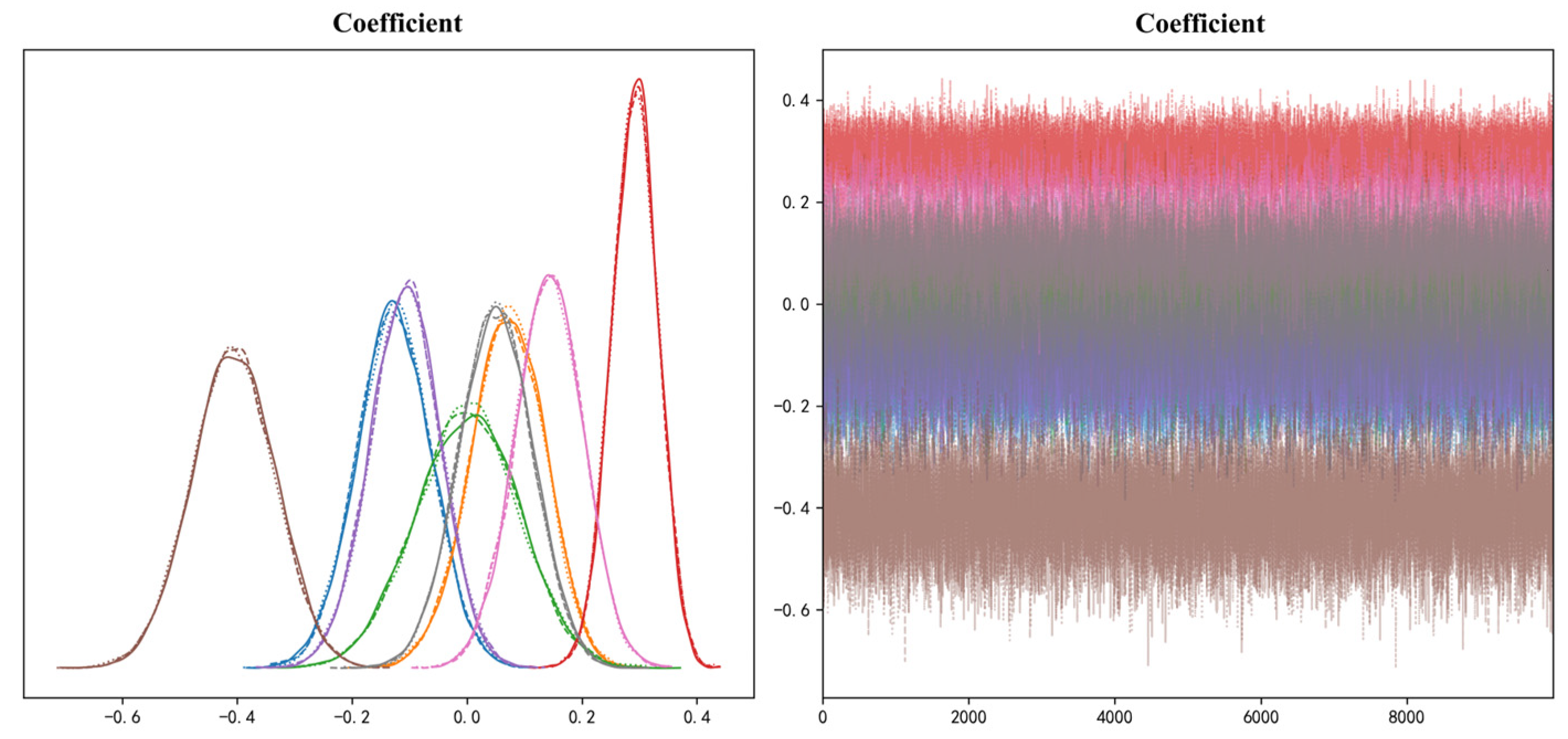
Negative Binomial Regression	314.91	334.03	129.84	41	3.1668	Not recommended (due to insufficient small-sample stability)

). While a negative binomial (NB) model can explicitly account for overdispersion, its dispersion parameter was estimated with high uncertainty (standard error > 0.5) due to our small sample size (n = 50), raising concerns about the stability of its estimates. However, priors can effectively stabilize coefficient estimates in small samples (n = 50) by avoiding extreme parameter values caused by overdispersion. The convergence of the BPR model was validated by R-hat < 1.01 and ESS > 20,000, and the predictive accuracy was confirmed by WAIC = 493.24.

The prior specification was strictly implemented in PyMC3, with the intercept term assigned a normal prior with a mean of 0 and a variance of 5², while all slope coefficients were assigned normal priors with a mean of 0 and a variance of 2². This prior structure avoids over-constraining the intercept term and ensures full consistency between the mathematical formulation and the computational implementation.

3.5. Variable Selection

For the unit of analysis, we use the spatial unit of traffic analysis zones (TAZs), which are widely employed in transportation analysis [37]. On the basis of previous research and data availability, we divided the study area into 50 traffic districts. The average area of each traffic district is 0.37 km², and the biggest area is 1.71 km². This study used the frequency of older adult-involved traffic crashes per traffic zone as the dependent variable.

As shown in

Table 2. Definitions of variables.

Independent Variables		Definitions
Density	Population	Total population/TAZ area
	Older population	Total older population/TAZ area
	Employment	Total employed population/TAZ area
	Retail facility	No. of retailing facilities/TAZ area
	Educational facility	No. of schools/TAZ area
	Medical facility	No. of hospitals/TAZ area
	Recreational facility	No. of recreational facilities/TAZ area
	Public transport stop density	No. of bus stops/TAZ area
Design	Intersection	No. of intersections/TAZ area
	Road network	Total length of roads/TAZ area
	Footbridge	No. of footbridges/TAZ area
	Pedestrian underpass	No. of pedestrian underpasses/TAZ area
	Crosswalk	No. of crosswalks/TAZ area
Diversity	Land use mix	Measured by the Shannon Diversity Index
	Commercial	Area of commercial land/TAZ area
	Residential	Area of Residential land/TAZ area
	Parks and green spaces	Area of park and green space/TAZ area
	Public service	Area of public service facilities/TAZ area
	Industrial	Area of industrial land/TAZ area
	Road Traffic	Area of road traffic land/TAZ area
	Storage	Area of storage land/TAZ area

, the independent variables were categorized into three types, specifically density, design, and diversity. Density-related variables measure the degree of spatial agglomeration of various elements, including demographic factors and major destination facilities; design-related variables reflect the characteristics of the road environment; diversity-related variables characterize the mix and composition of land use functions (Figure 3). Regions with high population density, employment density, and activity facility density typically exhibit significantly elevated pedestrian flows and increased traffic volume, consequently heightening the likelihood of pedestrian–vehicle collisions [38]. Areas with greater older population density demonstrate increased traffic exposure among older adults, correspondingly raising their accident risk. Furthermore, pedestrian collisions involving older individuals predominantly occur near key destination facilities that support their daily activities, including essential living amenities and public transportation hubs. Therefore, this study incorporates the following density indicators: retail facility density, educational facility density, medical facility density, recreational facility density, and public transport stop density.

Road environmental variables included intersection density, road network density, crosswalk density, and the density of underground passages and pedestrian overbridges. Higher intersection density is associated with a greater likelihood of pedestrian collisions [39]. However, some studies also suggest that increased intersection density may actually reduce collision rates [40], as drivers tend to concentrate their attention more when approaching road junctions, thereby decreasing the probability of accidents at intersections. Higher road network density tends to increase traffic flow, consequently compromising older pedestrians’ travel safety [22]. At signal-controlled crosswalks, older pedestrians typically exhibit slower walking speeds than average [41]. Pedestrian signal timing that fails to accommodate older pedestrians’ needs, combined with excessively wide roadways, prevents seniors from completing crossings within safe time intervals, thereby elevating their accident risks [42]. In addition, in view of the undulating terrain, underpasses and pedestrian footbridges are common vehicular–pedestrian separation facilities in mountain cities, aiming to alleviate ground traffic pressure and reduce pedestrian–vehicle conflict points.

In terms of land use, we identified land use mix and the proportion of land use types. Land use mix (or mixed-use index) refers to a metric that quantifies the spatial integration of diverse functional land types within a given area. We calculated the land use mix for each traffic analysis zone (TAZ). To comprehensively characterize the land use patterns in our study area, we incorporated three specialized variables beyond conventional urban land categories (commercial, residential, park, and green space): (1) industrial land ratio, (2) road traffic land ratio, and (3) storage land ratio. This selection specifically addresses the unique spatial configuration of the study area.

The variable screening process consists of three sequential steps designed to ensure robustness and avoid multicollinearity. First, we perform Pure Poisson LASSO variable selection. The ElasticNetCV 1.7.2 tool (with l1_ratio = 1 for pure LASSO) is utilized to automatically select variables with non-zero coefficients. A 3-fold cross-validation was adopted to determine the optimal regularization parameter (α), given the small sample size (n = 50). Second, VIF-based multicollinearity diagnosis is conducted. The Variance Inflation Factor (VIF) of the selected variables is calculated with a threshold set at 10. Variables with values exceeding this threshold are excluded. Third, variable number adjustment is carried out. If an excessive number of variables were eliminated in the preceding steps, additional variables with the highest correlation with crash counts are supplemented to ensure sufficient model degrees of freedom. If relatively few variables were eliminated earlier, no elimination is performed in this step.

4. Results

4.1. Descriptive Statistics

Table 3. Descriptive statistics for the dependent and independent variables.

Variables			Obs	Min	Max	Mean	Std.Dev
Dependent Variable		Older-pedestrian crashes	50	0.00	33.00	7.78	7.83
Independent Variables	Density	Population density (persons/km2)	50	6463.42	359,859.18	107,118.08	83,608.22
		Older population density (persons/km2)	50	56.61	5619.74	1488.35	1304.32
		Employment density (persons/km2)	50	5389.49	468,959.04	101,062.96	85,675.45
		Retail facility density (pcs/km2)	50	0	327.89	85.56	77.99
		Educational facility density (pcs/km2)	50	0	71.88	10.57	13.76
		Medical density (pcs/km2)	50	0	141.24	37.32	41.37
		Recreational facility (pcs/km2)	50	0	136.73	25.07	28.25
		Public transport stop density (pcs/km2)	50	0	47.92	14.43	11.72
	Design	Intersection (pcs/km2)	50	5.25	1656.16	260.14	354.25
		Road network (pcs/km2)	50	0.26	84.68	17.4	17.96
		Footbridge (pcs/km2)	50	0	55.91	5.32	10.25
		Pedestrian underpass (pcs/km2)	50	0	66.61	7.05	12.83
		Crosswalk (pcs/km2)	50	0	143.76	26.61	34.33
	Diversity	Land use mix	50	0.05	0.7	0.42	0.19
		Commercial (km2/km2)	50	0	0.97	0.31	0.34
		Residential (km2/km2)	50	0	0.96	0.36	0.3
		Parks and green spaces (km2/km2)	50	0	0.51	0.1	0.15
		Public service (km2/km2)	50	0	0.98	0.19	0.19
		Industrial (km2/km2)	50	0	0.54	0.02	0.08
		Road Traffic (km2/km2)	50	0	0.55	0.02	0.08
		Storage (km2/km2)	50	0	0.06	0	0.01

shows the descriptive statistics of dependent and independent variables in the study. There are 50 traffic analysis zones (TAZs) in total, with the average number of older-pedestrian crashes per traffic zone being 7.78 and the highest number of incidents in a single zone reaching 33.

Figure 4 reveals that most older-pedestrian crashes in the study area are concentrated in three primary clusters. According to demographic data and field surveys, these zones not only have a higher density of older adults but also feature more complex built environments. Cluster A and Cluster C are situated within Chongqing’s historic urban core, once central to the city’s economic growth. These areas are characterized by dense residential communities, aging housing complexes, intricate street networks, and heavy pedestrian traffic—all of which increase accident likelihood. Additionally, ongoing urban renewal projects in these districts introduce construction-related disruptions, further exacerbating mobility challenges for older pedestrians. In contrast, Cluster D and Cluster E—Chongqing’s wholesale market hubs—primarily serve commercial functions, resulting in lower older-pedestrian activity. Similarly, Cluster F, a newer residential zone, benefits from well-planned transportation infrastructure and age-friendly facilities, leading to fewer and more spatially dispersed accidents.

The analysis further identifies two key risk factors in high-incident zones: Facility-rich urban areas with high residential density and concentrated older populations, such as Site A, demonstrate significantly higher expected crash rate, establishing them as critical safety hotspots. Complex road networks (e.g., Site B) also pose elevated risks, where inadequate pedestrian infrastructure—such as missing crosswalks, footbridges, or underpasses—compromises safety for older adults. This spatial distribution underscores the need for targeted urban interventions in high-risk zones to enhance older-pedestrian safety.

4.2. Model Estimation Results

4.2.1. Poisson Regression Model

The Poisson Regression model is one of the basic models for regression analysis of crash counts, suitable for describing the number of random events occurring per unit of time or space. During the construction of the Standard Poisson Regression model, the study first screened built environment variables to address multicollinearity and weak correlation issues. Based on the screening criteria, eight core collinearity-free indicators were retained for final modeling (all VIF < 3.1), including land use mix, recreational facility density, medical facility density, proportion of warehousing land, public transport stop density, educational facility density, footbridge density, and proportion of park and green space (

Table 4. Variable VIF results (all ≤ 10).

Variable	VIF
Land use mix	1.58
Recreational facility density	2.00
Medical facility density	3.01
Proportion of storage land	1.08
Public transport stop density	1.58
Educational facility density	2.18
Footbridge density	1.56
Proportion of park and green space	1.56

).

Table 5. The results of the Poisson Regression model.

Dependent Variable	Regression Coefficient	Standard Error	p-Value	Incidence Rate Ratio (IRR)	Significance
Land use mix	−0.6902	0.3487	0.0478	0.5015	*
Recreational facility density	0.0026	0.0023	0.2571	1.0026	ns
Medical facility density	0	0.0022	0.9982	1	ns
Proportion of storage land	26.8956	3.6371	0	4.79 × 1011	***
Public transport stop density	−0.0094	0.0053	0.0779	0.9907	.
Educational facility density	−0.0298	0.0053	0	0.9707	***
Footbridge density	0.0143	0.0058	0.0143	1.0144	*
Proportion of park and green space	0.3579	0.4467	0.423	1.4303	ns

Note: Sample size n is 50, and the number of explanatory variables k is 8, with one constant term. The residual degrees of freedom is 41. *** means significant at 1% level and * indicates significant at 10% level, ns denotes not significant.

shows the analysis of the Poisson Regression model for older-pedestrian crashes. The model estimates parameters and calculates the incidence rate ratio (IRR), which quantifies the multiplicative change in accident frequency per unit increase in an independent variable. IRR indicates that every time the built environment variable changes by one unit, the number of traffic accidents involving older pedestrians will change by IRR-1 times. The parameter estimation results of the Standard Poisson Regression model showed that older-pedestrian traffic crashes were significantly correlated with land use mix, public transport stop density, educational facility density, and footbridge density. No significant relationships were found between crashes and recreational facility density, medical facility density, or proportion of park and green space. The incidence rate ratio (IRR) for the proportion of storage land is anomalous, and subsequent interpretation thereof requires caution.

4.2.2. Bayesian Poisson Regression Model

Based on the significant built environment factors identified in the initial Poisson Regression analysis, this study further employed a Bayesian Poisson Regression (BPR) model to improve parameter estimation robustness. Modeling was implemented via PyMC3, with posterior analysis conducted using ArviZ. Weakly informative priors were specified, with the constant term β₀~N (0, 5²) and explanatory variable coefficients βᵢ~N (0, 2²), which avoids prior dominance over the data while providing regularization to stabilize estimates in our small sample. MCMC sampling was configured with three chains, each consisting of 2000 burn-in iterations and 10,000 sampling iterations, resulting in a total of 30,000 samples. Convergence was validated using R-hat (<1.01) (

Table 6. Bayesian Poisson Regression (BPR) model posterior results.

Variables	Posterior Mean	Posterior Standard Deviation	95% HDI Lower Bound	95% HDI Upper Bound	R-Hat (Convergence)	Effective Sample Size	Posterior IRR	IRR 95% CI
CONSTANT	1.7641	0.0551	1.6564	1.8723	1	32,279.703	5.8363	[5.2404, 6.5032]
Land use mix	−0.1272	0.0648	−0.2593	−0.0055	1	26,122.7918	0.8806	[0.7716, 0.9945]
Recreational facility density	0.0702	0.0651	−0.0565	0.1978	1.0001	26,540.4543	1.0727	[0.9451, 1.2187]
Medical facility density	0.0007	0.0895	−0.1819	0.1691	1	21,004.484	1.0007	[0.8337, 1.1842]
Proportion of storage land	0.2916	0.04	0.2138	0.369	1.0001	28,584.3791	1.3386	[1.2384, 1.4463]
Public transport stop density	−0.1077	0.0615	−0.2308	0.0112	1.0002	25,643.9987	0.8979	[0.7939, 1.0113]
Educational facility density	−0.4071	0.0726	−0.5492	−0.2653	1	23,898.4003	0.6656	[0.5774, 0.7670]
Footbridge density	0.1427	0.059	0.0291	0.2583	1	27,682.9895	1.1534	[1.0295, 1.2947]
Proportion of park and green space	0.0499	0.0642	−0.0768	0.1744	1	23,644.3323	1.0512	[0.9261, 1.1905]

Note: Priors implemented in PyMC3 exhibited a normal distribution with a mean of 0 and a variance of 5² for the intercept term β₀, as well as normal distributions with a mean of 0 and variance of 2² for all slope coefficients β_j.

), effective sample size (ESS > 1000), and trace plots (Figure 5), indicating good model convergence. Predictive accuracy was evaluated using WAIC (493.2352 ± 68.1078). Regression coefficients from both the Standard Poisson Regression (SPR) and the Bayesian Poisson Regression (BPR) models exhibited strong agreement, validating the initial findings. Compared to the SPR model, the BPR model exhibits smaller standard deviations for built environment variables. A smaller standard deviation indicates more precise coefficient estimates, suggesting that the sample data provides stronger support for the association coefficients between built environment variables and elderly pedestrian accident risk. Conversely, a larger standard deviation implies greater uncertainty in the coefficient estimates, potentially leading to less stable results. Therefore, the results of the Bayesian Poisson Regression (BPR) model are prioritized for subsequent mechanistic interpretation and policy impact analysis.

Table 7. Bayesian Poisson Regression (BPR) model summary results.

Variables	25th Percentile (Standardized)	75th Percentile (Standardized)	Percentile Difference (Standardized)	Bayesian Posterior Coefficient	Crash Rate Change (%)	Statistical Significance	Practical Significance
Land use mix	−0.69926	0.751524	1.450786	−0.1272	−16.8513	***	Practically Significant (>5%)
Recreational facility density	−0.65535	0.228262	0.883608	0.0702	6.399353	ns	Practically Significant (>5%)
Medical facility density	−0.76525	0.583657	1.348903	0.0007	0.094468	ns	Not Practically Significant (<5%)
Proportion of storage land	−0.2038	−0.2038	0	0.2916	0	***	Not Practically Significant (<5%)
Public transport stop density	−0.73582	0.455712	1.191534	−0.1077	−12.0435	ns	Practically Significant (>5%)
Educational facility density	−0.61166	0.127687	0.739342	−0.4071	−25.9912	***	Practically Significant (>5%)
Footbridge density	−0.52465	−0.04488	0.479775	0.1427	7.086201	***	Practically Significant (>5%)
Proportion of park and green space	−0.69884	0.451695	1.150531	0.0499	5.909155	ns	Practically Significant (>5%)

Note: *** means significant at 1% level, ns denotes not significant.

shows the results of the Bayesian Poisson Regression (BPR) model. This study simultaneously focuses on statistical significance (95% confidence interval [CI] excluding 0) and practical significance (crash rate change ≥ 5%). The results show that three variables exhibit both types of significance: land use mix (−16.85%), educational facility density (−25.99%), and footbridge density (7.09%). This indicates their effects are not only statistically reliable but also have practical planning implications. Furthermore, while recreational facility density (6.40%), public transport stop density (−12.04%), and proportion of park and green space (5.91%) are practically significant, they lack statistical significance and can be regarded as secondary optimization directions. Variables such as the proportion of storage land and medical facility density have minimal effects (<5%), rendering them of no practical planning value.

This study tested the spatial autocorrelation of regression residuals using Moran’s I test (

Table 8. Moran’s I test table.

Indicator	Value
Moran’s I	0.443
Expected Moran’s I	−0.0204
Z-statistic	5.2803
p-value	<0.0001
Conclusion on Spatial Autocorrelation	Significant Positive Autocorrelation (Residual Clustering)

), with spatial relationships defined by a Queen Contiguity Matrix. The result (Moran’s I = 0.443, p < 0.001) indicates significant positive spatial autocorrelation, meaning that the unexplained component of crash risk exhibits a clustered pattern across nearby TAZs. This suggests that unobserved risk factors are themselves spatially dependent. For the non-spatial models (SPR and BPR) used here, such residual spatial dependence implies that the reported standard errors of coefficients may be underestimated, and the associated parameter uncertainties should therefore be interpreted with caution. Consequently, while the models provide valuable insights, policy inferences drawn from them should be tempered by the recognition of this underlying spatial structure.

5. Discussion

5.1. Key Findings and Interpretation

This study provides empirical evidence on how built environment characteristics influence traffic crash risks for older pedestrians, revealing the complex relationships between the built environment and pedestrian safety—with some findings challenging conventional assumptions. Analyses based solely on crash counts may obscure the inherent heterogeneity of risk structures, requiring comprehensive interpretation integrating dimensions such as crash frequency and severity, as well as social and transportation system risks [43,44].

5.1.1. Land Use Impacts

This study found that both land use mix and the proportion of park and green space are associated with older-pedestrian crash risks. When land use mix increases from a typical low level (25th percentile) to a typical high level (75th percentile), the crash rate is projected to decrease by approximately 16.85%. This indicates that enhanced land use mix contributes to the walking safety of older adults [20], as diversified urban land use can reduce the travel distance and time of older adults, thereby lowering traffic accident risks [45]. This reflects the positive effect of functionally integrated urban environments in suppressing traffic conflicts through spatial integration. Similarly, while the proportion of park and green space is not statistically significant, increasing from a typical low level (25th percentile) to a typical high level (75th percentile) is projected to increase the crash rate by approximately 5.91%, slightly exceeding the 5% threshold. This yields a counterintuitive result inconsistent with the existing literature [46]. However, it should not be interpreted as the proportion of park and green space having a slight practical negative impact on older-pedestrian crash risks. Conversely, concluding that park and green space should be reduced is highly unreasonable. The correct interpretation is that park and green space areas may attract more older pedestrians, thereby increasing traffic accident risks. In short, claiming or denying that the proportion of park and green space increases crashes based solely on aggregated traffic data is questionable.

5.1.2. Facility Density and Pedestrian Safety

When educational facility density increases from a typical low level (25th percentile) to a typical high level (75th percentile), the crash rate is projected to decrease by approximately 25.99%. In China, older adults often take on the responsibility of picking up and dropping off their grandchildren from school [15]. Despite heavy traffic around schools, strict speed limits, parking control measures, and pedestrian–vehicle separation facilities (e.g., barriers) collectively create a safer environment. Notably, areas around kindergartens and primary/secondary schools—where older pedestrians gather—exhibit lower accident rates. This phenomenon underscores the importance of strengthening pedestrian safety measures: high-traffic areas with strict management and well-designed infrastructure can effectively reduce collision risks. When recreational facility density increases from a typical low level (25th percentile) to a typical high level (75th percentile), the crash rate is projected to increase by approximately 6.40%. Recreational facilities attract pedestrians, especially older adults, who may walk around without paying special attention to traffic and feel safer in crowded areas, thus lowering their vigilance and inadvertently increasing accident probabilities [15]. Simply increasing recreational facilities without supporting speed reduction designs or crossing protection may inadvertently raise conflict frequencies. When public transport stop density increases from a typical low level (25th percentile) to a typical high level (75th percentile), the crash rate is projected to decrease by approximately 12.04%. This indicates that the lack of infrastructure such as bus stops may increase older adults’ walking opportunities and time, thereby raising accident probabilities [47]. In contrast, areas around stops are usually equipped with pedestrian crossing facilities and management, forming nodal protection.

5.1.3. Pedestrian Infrastructure Efficacy

A defining characteristic of mountainous cities is significant topographic relief. In this context, pedestrian footbridges play a crucial multidimensional role—not only as physical carriers connecting spaces but also as one of the most effective measures to achieve complete physical separation between pedestrians and vehicles. However, pedestrians often exhibit a tendency to avoid using footbridges when crossing roads, increasing the likelihood of pedestrian-involved accidents [48]—a phenomenon particularly pronounced among older adults with walking difficulties. The study results show that when footbridge density increases from a typical low level (25th percentile) to a typical high level (75th percentile), the crash rate is projected to increase by approximately 7.09%, indicating that footbridge density has a significant inhibitory effect on older pedestrians’ safety. Field investigations in the study area revealed that due to the significant topographic relief of mountainous cities, the current age-friendly design of footbridges is insufficient to meet pedestrians’ crossing needs—with a lack of elevators—and older residents particularly report difficulties in crossing roads.

5.2. Policy Implications

Based on the empirical evidence of this study, the following policy recommendations are proposed to translate research findings into actionable urban planning interventions for improving older-pedestrian safety in mountainous cities:

• Policy 1: Optimization of Built Environment Land Use

Reduce older adults’ daily walking distance and lower exposure risks. It is recommended to enhance land use mix based on the characteristics of older adults’ activity circles and implement a gradient mixed land use layout. Specifically, promote the integration of residential, convenient service, and medical functions within 5 min walkable areas; strengthen the mix of commercial, health, and public space functions within 10 min walkable areas; and guide the formation of comprehensive commercial, cultural, and green space nodes within 15 min walkable areas. Through compact and integrated land use organization, effectively shorten older adults’ daily travel distance. For public green spaces such as parks and squares, focus on optimizing the connection safety between green spaces and surrounding road networks. Ensure direct access between green space entrances/exits and safe, accessible crossing facilities, and implement strict traffic calming designs on connecting roads to reduce potential risk exposure.

• Policy 2: Layout and Density Regulation of Living Service Facilities

When intensifying the layout of schools and public transport stops, delineate safety zones around schools and mandate the supporting construction of sidewalk barriers, clear crossing signs, speed limit, and illegal parking monitoring facilities. At public transport stops, ensure safe and comfortable waiting areas with convenient access to the nearest signal-controlled crossing facilities. Near leisure facilities such as commercial centers, squares, and senior activity centers, the design of venue entrances/exits and pedestrian flow distribution spaces must be coordinated with traffic organization to avoid direct conflicts between pedestrian and vehicle flows. For existing built-up areas, supplementary pedestrian warning signs, mandatory speed reduction facilities, and crossing protection devices must be installed to mitigate potential risks.

• Policy 3: Footbridge Expansion Program

Conduct a systematic assessment of traffic conditions across different road types, prioritizing the construction of pedestrian footbridges on secondary roads with high pedestrian and vehicle volumes. To enhance the safety of older pedestrians, propose the creation of “Silver Pedestrian Corridors” along these secondary roads, featuring accessible footbridges with gentle slopes and rest platforms. Upgrade these footbridges with elevators to improve age-friendliness and integrate IoT-based monitoring systems to optimize facility layout.

5.3. Limitations

This study has several limitations that should be noted. First, the cross-sectional design prevents establishing causal relationships, while reliance on reported crash data likely underestimates minor incidents particularly relevant for older pedestrians. Second, the single-city focus may limit generalizability to other urban contexts with different infrastructure and traffic patterns. Third, this study adopts a non-spatial Bayesian Poisson model that does not consider spatial spillover effects between TAZs, potentially underestimating parameter uncertainty. Future research could introduce spatial Bayesian models and incorporate spatial weight matrices into modeling to further improve result reliability.

6. Conclusions

The travel safety of older adults has become a critical issue in contemporary society. Numerous studies on the built environment have sought to enhance pedestrian safety for older adults; however, many fail to account for parameter uncertainty, limiting their ability to provide a comprehensively safe walking environment. Building upon previous research, this study further investigates the factors influencing pedestrian–vehicle collisions among older adults, with the aim of reducing accident frequency by examining built environment characteristics. The key findings are as follows:

In the Standard Poisson Regression model analysis, public transport stop density was significant at the 10% level, while land use mix and footbridge density were significant at the 5% level. Educational facility density exhibited significance at the 1% level. Notably, neither recreational facility density nor medical facility density had a significant impact on the frequency of traffic accidents involving older pedestrians.

The Bayesian Poisson Regression model revealed that footbridge density, recreational facility density, and the proportion of park and green space were positively correlated with accident frequency. This indicates that higher densities of these facilities may reduce the travel safety of older pedestrians. Conversely, land use mix, educational facility density, and public transport stop density were negatively correlated with accident frequency, suggesting that increased densities of these elements help enhance the safety of older pedestrians.

Based on these findings, we propose enhancing land use mix and implementing a gradient mixed land use layout, optimizing the layout of schools and public transport stops and improving safety facilities around leisure facilities, and prioritizing the construction of accessible footbridges with rest platforms on secondary roads. This multidimensional aging-friendly transportation improvement plan aims to support active transportation planning with older adult engagement. Future research should further analyze the dataset used in this study to validate and expand upon these findings.