Research on Aerodynamic Loads Caused by Maglev Train Entering Tunnels Under Crosswinds

Featured Application

This study provides a theoretical basis for the aerodynamic characteristics and safety of maglev trains entering tunnels under crosswind conditions.

Abstract

Strong crosswinds and train–tunnel aerodynamic interactions cause the aerodynamic loads acting on the train body to change more drastically when a high-speed maglev train enters a tunnel. This greatly raises the risk of safety incidents like derailment or overturning. This study employs the FLUENT 2023 R2 computational fluid dynamics simulation software with an overset grid method to numerically investigate the influence patterns of crosswinds on aerodynamic loads and relevant safety issues for a 600 km/h maglev train entering tunnels under various crosswind conditions. The findings show that (1) the marshaling location has a strong correlation with aerodynamic performance. When there is no crosswind, the head vehicle (HV) has the greatest chance of flipping, while the rear vehicle (RV) has the worst lift characteristics. All three vehicles experience significant sudden changes in lateral force coefficients prior to tunnel entry, indicating considerable derailment risks. (2) Aerodynamic loads on the HV show significantly greater sensitivity to crosswind velocity variations compared to the middle vehicle (MV) and RV, with the amplitude reduction in lateral forces in the HV showing approximately linear increase with wind speed. (3) A 50 km/h reduction in train speed decreases the amplitude of change in the lift coefficient and lateral force coefficient by approximately 4.8% and 8.9%, respectively, and the peak overturning moment in open air and tunnel by approximately 11.4% and 15.7%, respectively. These discoveries have both practical value for advancing high-speed maglev networks and theoretical significance for enhancing the safety and reliability of Chinese maglev systems.

1. Introduction

Maglev transportation, a typical example of modern rail transit technology, has the advantages of high operating speeds, non-mechanical contact wear, and environmental friendliness. Its operational safety and stability, however, still need a lot of investigation to be confirmed. The aerodynamic load experienced by high-speed trains during operation is approximately proportional to the velocity raised to the power of 0.46–0.60 [1]. The high-speed trains generate an extreme aerodynamic environment when traveling through a tunnel [2], and high-speed maglev trains show more noticeable dynamic changes in aerodynamic loads during tunnel passages since they can reach speeds up to 600 km/h, which is far faster than traditional wheel-rail systems. On the other hand, the sudden changes in lateral forces caused by strong crosswinds significantly raise the danger of safety problems like derailment or overturning when high-speed trains pass through difficult terrain like coastal regions or high wind zones [3].

The current researchers mainly focus on the pressure between the train and the tunnel surface, the propagation laws of pressure waves, and the corresponding flow field distribution [4,5] when a 200–400 km/h high-speed rail track train enters a tunnel under crosswind conditions, as well as the sudden changes in aerodynamic loads [5,6,7]. Numerous scholars have investigated influencing factors on aerodynamic characteristics under crosswind conditions. For instance, Bocciolone et al. [8,9,10,11] studied varying crosswind attack angles, revealing pressure distribution patterns on train surfaces and aerodynamic force variations under different working conditions. Mei et al. studied the initial compression waves induced by a 400 km/h high-speed train entering a tunnel under both offset running and center running conditions [12]. Based on the one-dimensional compressible unsteady non-isentropic flow model and an improved generalized Riemann variable characteristic method, the propagation mechanism of initial compression waves under three portal shapes was investigated [13]. As for sudden changes in hydrodynamic characteristics of unsteady flow, Ershkov S.V. et al. conducted an extended investigation of the N-S equations employing a theoretical derivation approach [14]. The generalized Kelvin–Kirchhoff formulation provides a theoretical framework for describing the resultant hydrodynamic forces acting on a moving body in a fluid domain with time-varying flow conditions [15]. Wang et al. employed a combination of field tests and numerical simulations to investigate the characteristics of transient pressure loads and micro-pressure waves inside a tunnel during the passage of a 350 km/h high-speed train [16]. Brambilla et al. [17,18,19] conducted wind tunnel experiments and simulations to examine the effects of wind barriers and related parameters on high-speed train aerodynamics. Chen et al. [20] performed numerical simulations comparing single-track and double-track tunnels, investigating how track configurations influence aerodynamic characteristics during train entry/exit under crosswinds. Additionally, studies have addressed train encounters under crosswind conditions [21,22,23], as well as aerodynamic characteristics when trains transition between open terrain and bridge-tunnel structures [24,25,26,27].

In the field related to maglev trains entering tunnels, Yang et al. investigated the mechanism and mitigation effect of Helmholtz resonators with different configuration schemes on the amplitude of the micro-pressure wave at the tunnel exit during the operation of a 600 km/h maglev train [28]. Han et al. [29] studied the aerodynamic characteristics of maglev trains during encounters inside tunnels. Zhang et al. [30] investigated variations in pressure wave amplitudes and the influence of train speed on pressure waves during maglev train operation and encounters in tunnels. Tian et al. [31] investigated the effects of train speed and guideway clearance on maglev trains during encounters, subsequently proposing optimization measures for the guideway spacing based on these findings. Zhang et al. [32,33] studied an arched shell structure applied in tunnels to expand cross-sectional areas, which helps dissipate the energy of initial compression waves, and analyzed the mitigation effects of structure length on compression waves. Additionally, other scholars have explored the impacts of train speed [34] and aerodynamic loads on suspension components [35] on the aerodynamic behavior of maglev trains operating in tunnels.

However, research on the aerodynamic effects in tunnels for high-speed maglev trains often neglects the influence of crosswinds, while current studies on trains under crosswind conditions, both domestically and internationally, are predominantly focused on wheel-rail high-speed trains. In fact, existing aerodynamic theories applicable to wheel-rail systems operating below 400 km/h are inadequate for accurately describing the aerodynamic behavior of maglev systems traveling at 600 km/h. In tunnels located in strong wind areas, the coupled effect of intense crosswinds and tunnel aerodynamics can significantly amplify sudden changes in the aerodynamic loads on maglev trains, thereby increasing safety risks. To address this research gap, we systematically investigated the aerodynamic characteristics of maglev trains. In particular, the study compares safety risks across different vehicle components and examines potential hazards by analyzing the influence of crosswind direction and speed at the tunnel entrance on aerodynamic lift, lateral force, and overturning moment. This in-depth exploration of the aerodynamic effects when high-speed maglev trains enter tunnels under complex wind conditions not only offers practical insights for advancing the development of maglev transportation networks but also establishes a theoretical foundation for enhancing the safety and operational reliability of next-generation high-speed maglev systems.

2. Numerical Methodology

2.1. Governing Equations for Fluids

Given the operational speed of 600 km/h (Mach number ≈ 0.49) in this study, which exceeds the critical threshold of Mach 0.3, the compressibility effects of air cannot be neglected [11]. The airflow surrounding a train at 600 km/h is characterized as turbulent, owing to a Reynolds number well above the critical threshold [36]. The RNG k-ε two-equation turbulence model demonstrates robust capability in capturing transient flow phenomena and has been extensively validated in studies of train–tunnel aerodynamic interactions [37,38,39]. Accordingly, this research employs three-dimensional viscous, compressible Navier–Stokes equations coupled with the RNG k-ε turbulence model and standard wall functions to simulate the aerodynamic process of high-speed maglev trains entering tunnels. The continuity, momentum, and energy equations are given as Equations (1)–(3).

$${\displaystyle \frac{𝜕\rho }{𝜕t}}+{\displaystyle \frac{𝜕\left(\rho u\right)}{𝜕x}}+{\displaystyle \frac{𝜕\left(\rho v\right)}{𝜕y}}+{\displaystyle \frac{𝜕\left(\rho w\right)}{𝜕z}}=0$$

(1)

$$\left\{\begin{array}{c}{\displaystyle \frac{𝜕\left(\rho u\right)}{𝜕t}}+{\displaystyle \frac{𝜕\left(\rho u\cdot u\right)}{𝜕x}}+{\displaystyle \frac{𝜕\left(\rho u\cdot v\right)}{𝜕y}}+{\displaystyle \frac{𝜕\left(\rho u\cdot w\right)}{𝜕z}}={\displaystyle \frac{𝜕}{𝜕x}}\left(\mu {\displaystyle \frac{𝜕u}{𝜕x}}\right)+{\displaystyle \frac{𝜕}{𝜕y}}\left(\mu {\displaystyle \frac{𝜕u}{𝜕y}}\right)+{\displaystyle \frac{𝜕}{𝜕z}}\left(\mu {\displaystyle \frac{𝜕u}{𝜕z}}\right)-{\displaystyle \frac{𝜕P}{𝜕x}}+S_u\\ {\displaystyle \frac{𝜕\left(\rho v\right)}{𝜕t}}+{\displaystyle \frac{𝜕\left(\rho v\cdot u\right)}{𝜕x}}+{\displaystyle \frac{𝜕\left(\rho v\cdot v\right)}{𝜕y}}+{\displaystyle \frac{𝜕\left(\rho v\cdot w\right)}{𝜕z}}={\displaystyle \frac{𝜕}{𝜕x}}\left(\mu {\displaystyle \frac{𝜕v}{𝜕x}}\right)+{\displaystyle \frac{𝜕}{𝜕y}}\left(\mu {\displaystyle \frac{𝜕v}{𝜕y}}\right)+{\displaystyle \frac{𝜕}{𝜕z}}\left(\mu {\displaystyle \frac{𝜕v}{𝜕z}}\right)-{\displaystyle \frac{𝜕P}{𝜕y}}+S_v\\ {\displaystyle \frac{𝜕\left(\rho w\right)}{𝜕t}}+{\displaystyle \frac{𝜕\left(\rho w\cdot u\right)}{𝜕x}}+{\displaystyle \frac{𝜕\left(\rho w\cdot v\right)}{𝜕y}}+{\displaystyle \frac{𝜕\left(\rho w\cdot w\right)}{𝜕z}}={\displaystyle \frac{𝜕}{𝜕x}}\left(\mu {\displaystyle \frac{𝜕w}{𝜕x}}\right)+{\displaystyle \frac{𝜕}{𝜕y}}\left(\mu {\displaystyle \frac{𝜕w}{𝜕y}}\right)+{\displaystyle \frac{𝜕}{𝜕z}}\left(\mu {\displaystyle \frac{𝜕w}{𝜕z}}\right)-{\displaystyle \frac{𝜕P}{𝜕z}}+S_w\end{array}\right.$$

(2)

$${\displaystyle \frac{𝜕\left(\rho T\right)}{𝜕t}}+div\left(\rho uT\right)=div\left({\displaystyle \frac{k}{c_p}}gradT\right)+S$$

(3)

The governing equations for the RNG k-ε model are as follows: (4), (5), and (6).

$${\displaystyle \frac{𝜕\left(\rho k\right)}{𝜕t}}+{\displaystyle \frac{𝜕\left(\rho \overline{u_j}k\right)}{𝜕x_j}}={\displaystyle \frac{𝜕}{𝜕x_j}}\left[\left(\mu +{\displaystyle \frac{{\mu }_t}{{\sigma }_k}}\right){\displaystyle \frac{𝜕k}{𝜕x_j}}\right]+P_k+P_b-\rho \epsilon +S_k$$

(4)

$${\displaystyle \frac{𝜕\left(\rho \epsilon \right)}{𝜕t}}+{\displaystyle \frac{𝜕\left(\rho \overline{u_j}\epsilon \right)}{𝜕x_j}}={\displaystyle \frac{𝜕}{𝜕x_j}}\left[\left(\mu +{\displaystyle \frac{{\mu }_t}{{\sigma }_{\epsilon }}}\right){\displaystyle \frac{𝜕\epsilon }{𝜕x_j}}\right]+C_1{\displaystyle \frac{\epsilon }{k}}(P_k+C_3{P}_b)-C_2\rho {\displaystyle \frac{{\epsilon }^2}{k}}+S_{\epsilon }$$

(5)

$${\mu }_t=C_{\mu }{\displaystyle \frac{\rho k^2}{\epsilon }}$$

(6)

2.2. Geometric Model

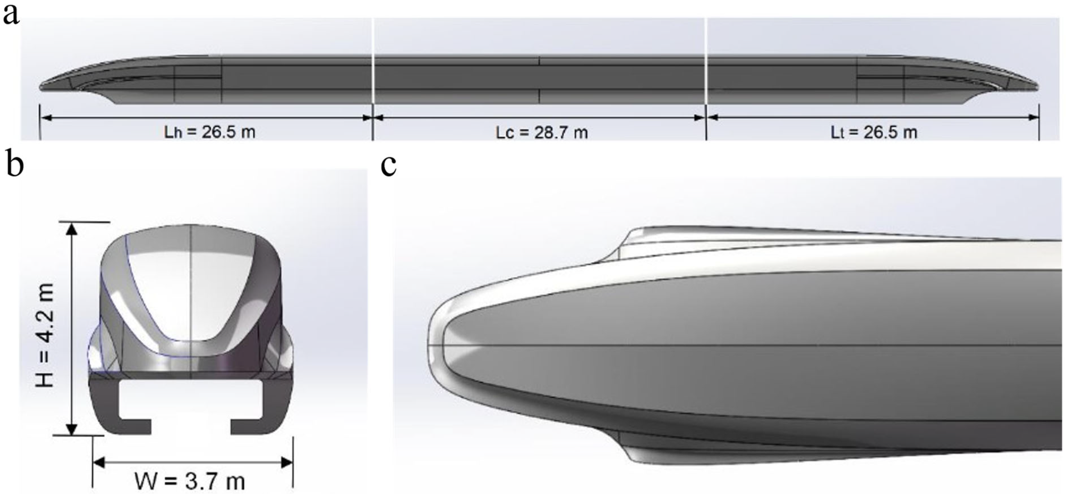
This study focuses on the CF600 high-speed maglev train as the research subject. The geometric model was developed using SolidWorks 2024, with subsequent geometry cleanup and feature simplification performed in Ansys SpaceClaim 2023 R2. To improve the calculation efficiency, the fine structures, such as the car door and the car lamp have been simplified. The finalized train geometry and dimensional specifications are presented in Figure 1:

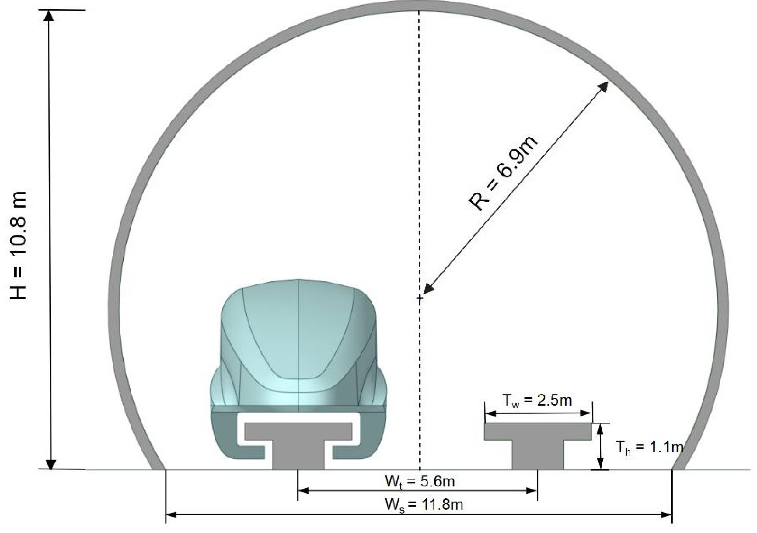
The three-dimensional models of the tunnel and guideway were constructed by using ANSYS SpaceClaim. The tunnel adopts a single-bore double-track configuration with a circular cross-section, featuring a blockage ratio of approximately 0.1 and a total length of 600 m. The guideway system employs T-shaped girders, with detailed geometric parameters illustrated in Figure 2:

2.3. Computational Domain and Meshing

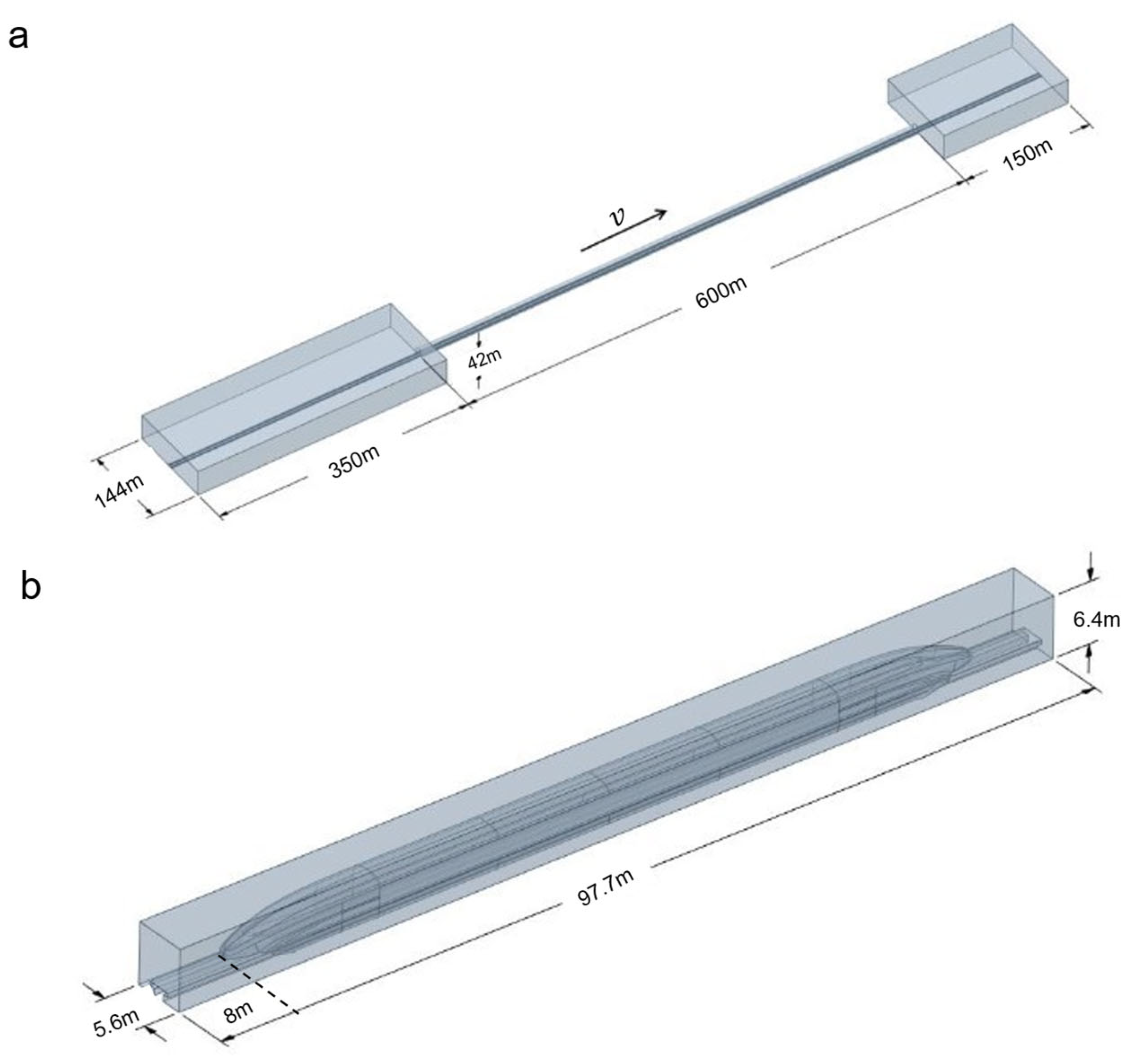
This study employs an overset mesh methodology to simulate the relative motion between the train and tunnel, thus partitioning the computational domain into a background region and a foreground region. The specific details of the background and foreground regions are shown in Figure 3a,b, respectively. Considering the size requirement of the overlap zone in the overset grid, the distance between both ends of the train and the corresponding boundaries of the foreground region is set to 8 m each.

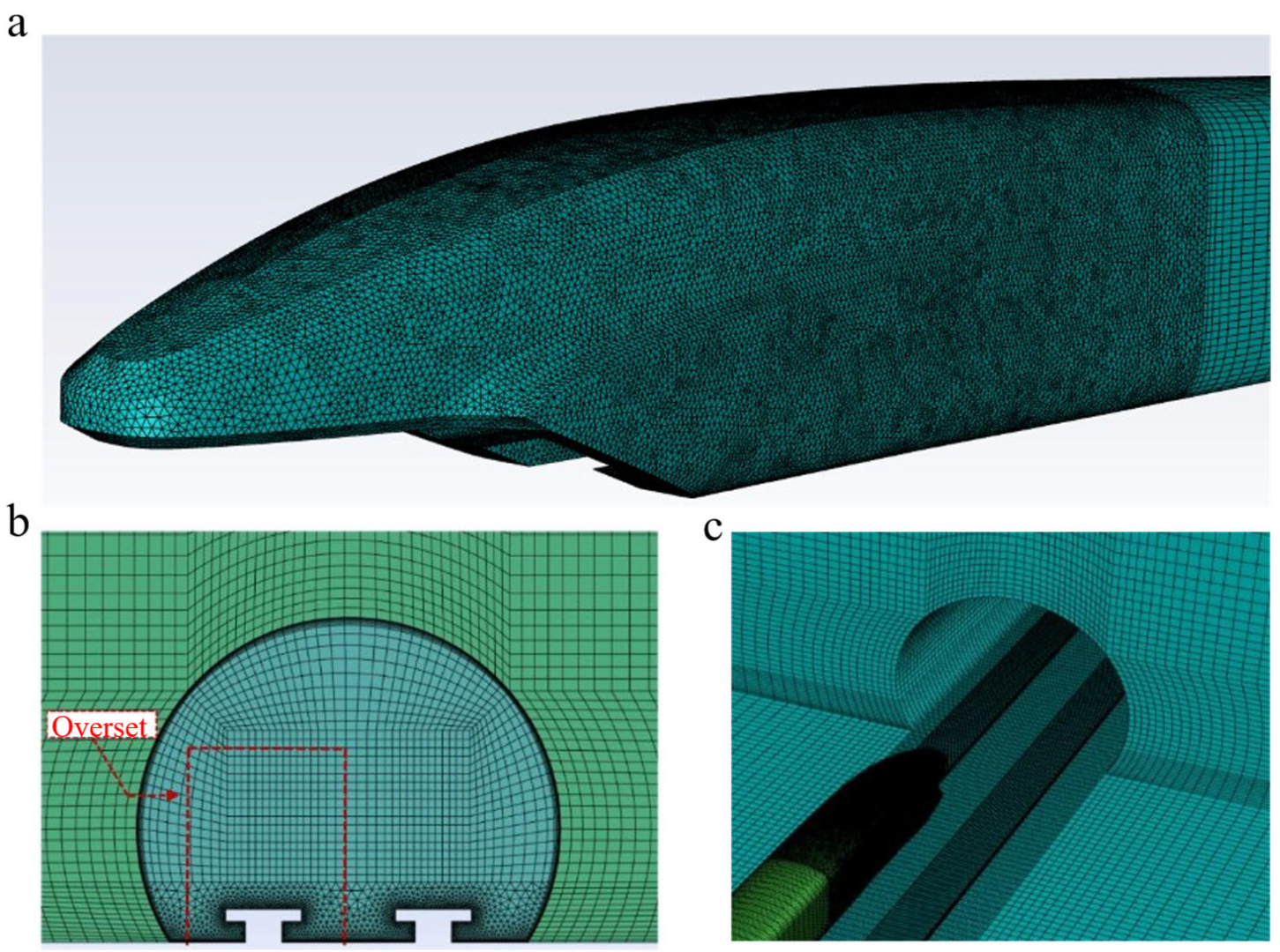
Commercial computational fluid dynamics (CFD) software is extensively employed to model a wide range of fluid flow, heat transfer, and mass transfer processes [40]. Within these software packages, ANSYS Mesh 2023 R2 serves as a crucial tool for generating computational grids. The mesh generation results are shown in Figure 4. The mesh discretization for the background area and the foreground area was carried out using ANSYS Mesh. The Multizone method can be defined as a type of blocking approach similar to ICEM-CFD. It employs automated topology decomposition to produce structured hexahedral meshes in regions where a suitable blocking topology exists [41]. In the background area, the MultiZone method was employed to divide the air domain and the upper part of the tunnel into hexahedral structured grids, the lower part of the tunnel into triangular prism grids, and the grids near the track into denser ones. To accurately capture the flow structure within the boundary layer of the tunnel walls, the boundary layer grids were divided on the tunnel walls and the ground. The height of the first layer of the boundary layer grids was set at 5 × 10⁻³ m, corresponding to y+ values ranging from 30 to 100, with a grid growth rate of 1.2, and a total of 7 layers of grids were set. The longitudinal grid size of the tunnel and the air domain was 0.5 m. The number of grids in the background area was approximately 10.6 million. The tetrahedral meshing method primarily generates computational grids composed of tetrahedral elements [41]. In the foreground area, the tetrahedral meshing method was used to divide the nose tips of the front and rear vehicles and the front and rear parts of the train body into tetrahedral unstructured grids to better capture the streamlined structure and details such as the guide slots; since the cross-sectional shapes of the rear and middle vehicles of the front and rear vehicles remained basically unchanged, the MultiZone method was used to divide the rear parts of the front and rear vehicles and the vehicle parts into triangular prism grids. The minimum size of the nose tip part of the grid was 0.02 m, the longitudinal grid size of the vehicle part was 0.5 m, and transitional grids were divided at the connection points between the two parts to ensure that the size ratio of adjacent grids was within a reasonable range. The boundary layer grids were also divided on the train surface to accurately capture the flow separation characteristics when the crosswind flows over the train surface. The height of the first layer of the boundary layer grids was set at 10⁻³ m, with a grid growth rate of 1.2, and a total of 11 layers of grids were set. The number of grids in the foreground area was approximately 3.5 million.

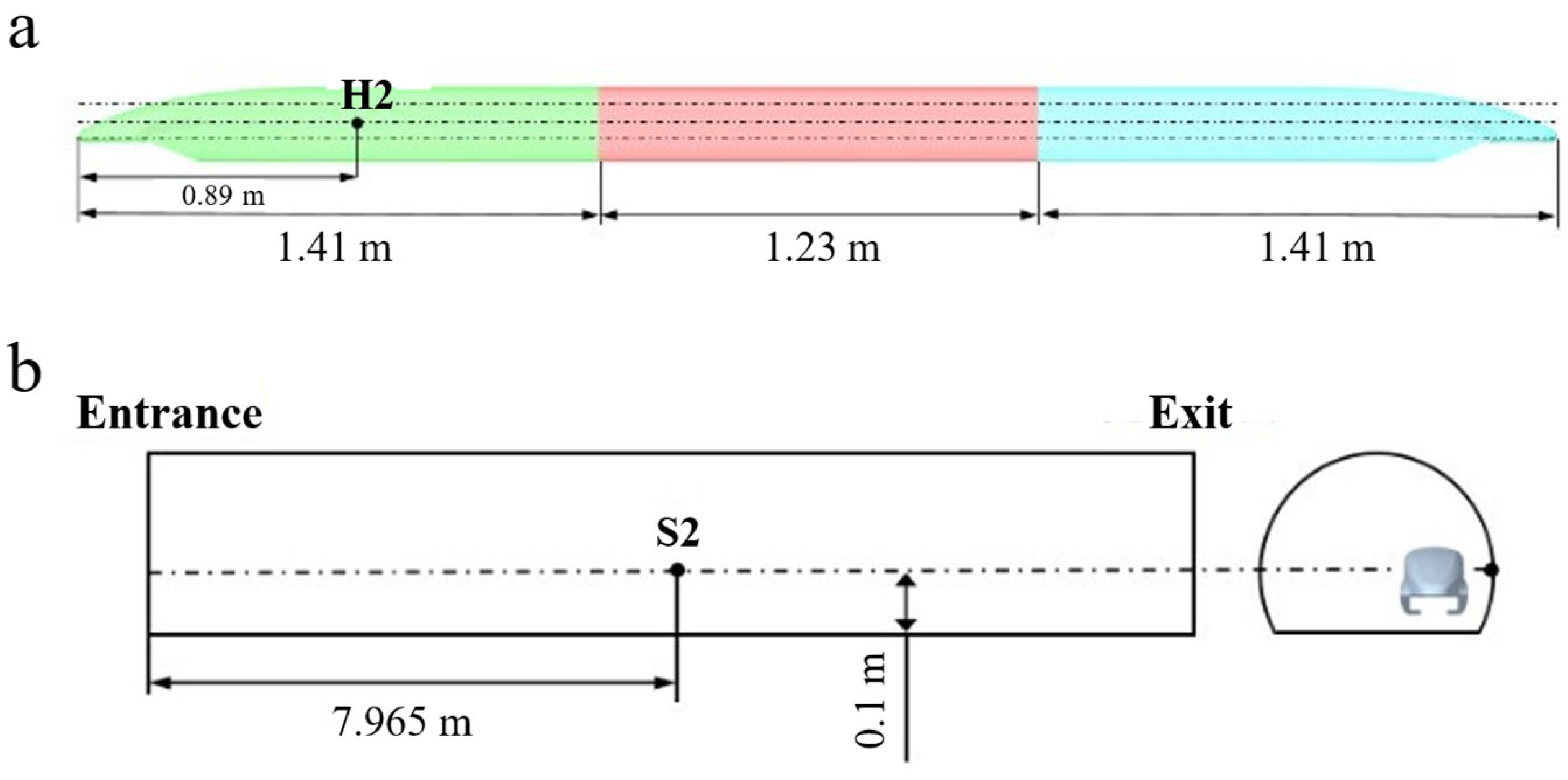
To verify the influence of grid size and time step selection on the numerical simulations, a grid and time step independence validation was conducted using the scenario of a high-speed maglev train entering a tunnel without crosswind as the benchmark case. Since this paper primarily focuses on the aerodynamic characteristics of the maglev train and the train–tunnel aerodynamic effects, the surface measurement point H2 on the train model and the wall measurement point S2 in the tunnel model are selected as representative locations. The positions of measurement points H2 and S2 are shown in Figure 5.

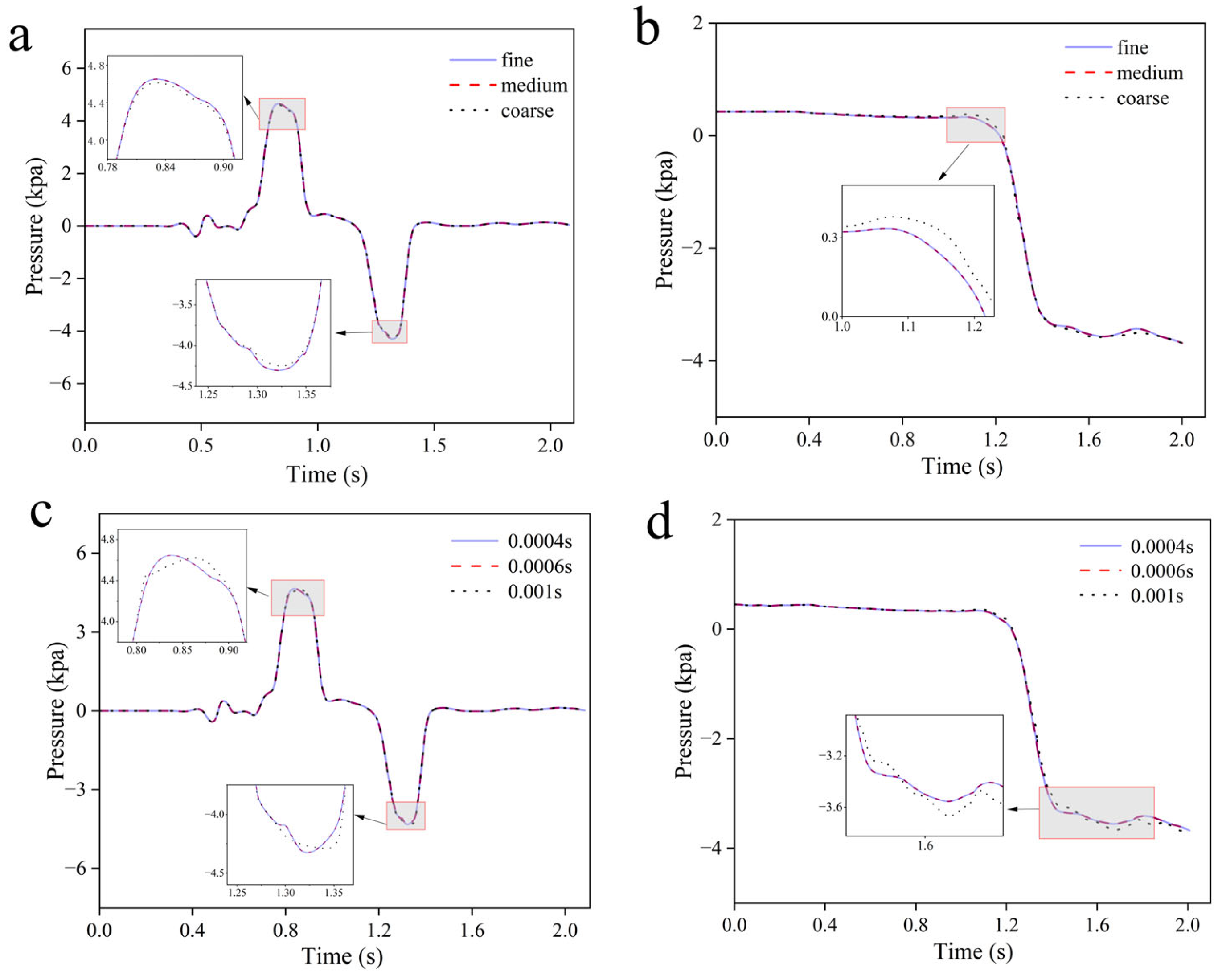
Three mesh configurations with identical topology but varying refinement levels (coarse, medium, and fine), as specified in

Table 1. Dimensions of meshes with different accuracies.

Mesh Type	Minimum Mesh Size		Number (Million)
	Train Surface	Tunnel Surface
coarse	0.03	0.50	9.50
medium	0.02	0.35	14.10
fine	0.01	0.20	21.90

, were employed for grid independence analysis. As shown in Figure 6a,b, which compare pressure time-history curves at monitoring points on the tunnel and train surfaces across the three mesh resolutions, deviations relative to the fine-mesh reference were quantified as follows: Coarse and medium meshes exhibited differences of 1.36% and 0.29% in tunnel wall positive pressure peaks, 2.67% and 0.02% in negative pressure peaks, and 1.83% and 0.01% in train surface pressure peak-to-peak amplitudes, respectively. Considering the balance between computational accuracy (medium mesh deviations ≤0.3%) and resource efficiency, the medium-resolution mesh configuration was selected for subsequent simulations.

Building upon the grid independence validation methodology, time step independence analysis was conducted using three temporal resolutions: 4 × 10⁻⁴ s, 6 × 10⁻⁴ s, and 1 × 10⁻³ s under identical operational conditions. As demonstrated by the pressure time-history curves at monitoring points on the tunnel and train surfaces in Figure 6c,d, the 1 × 10⁻³ s time step failed to resolve transient pressure variations during rapid flow transitions. Relative to the 4 × 10⁻⁴ s reference, deviations in pressure metrics were quantified as follows: 1 × 10⁻³ s and 6 × 10⁻⁴ s steps exhibited differences of 0.87% and 0.20% in tunnel wall positive pressure peaks, 1.12% and 0.19% in negative pressure peaks, and 5.86% and 0.15% in train surface peak-to-peak amplitudes, respectively. The 6 × 10⁻⁴ s time step was ultimately selected as the optimal temporal resolution, achieving an effective equilibrium between solution accuracy (maximum deviation ≤0.2% for critical metrics) and computational resource utilization efficiency.

2.4. Boundary Conditions and Solver Settings

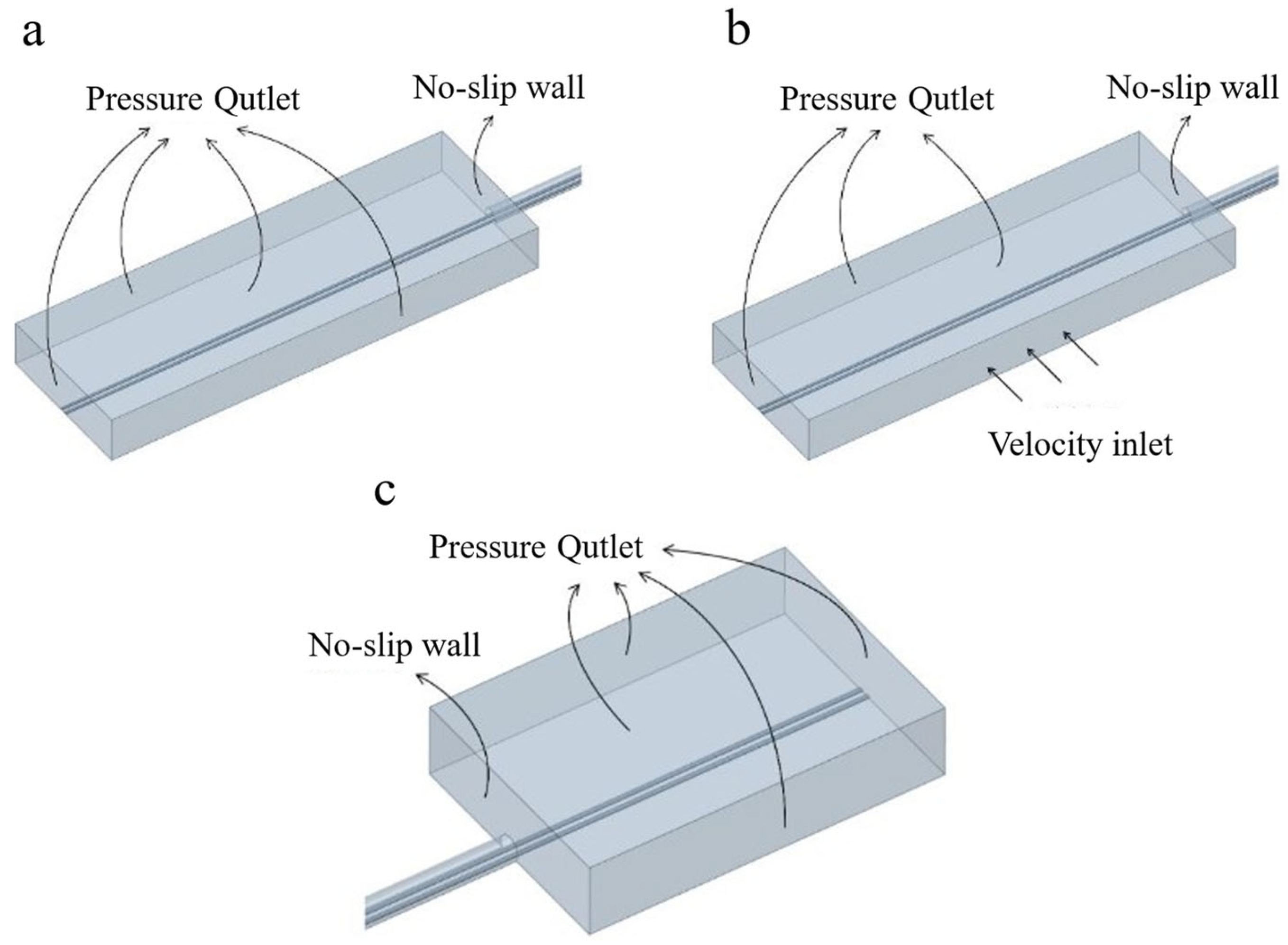
A comprehensive presentation of the boundary condition setup is provided below, with the specific configuration illustrated in Figure 7.

(1)

No-slip wall

The air domain boundaries at the train surface, tunnel walls, track surface, ground, and tunnel portal are all assigned the no-slip wall boundary condition with friction. The equivalent sand-grain roughness height for the train surface is specified as 0.045 mm, while that for the other no-slip walls is set to 5 mm. All no-slip walls are given the second-type boundary condition, with a heat flux density of 0 W/m².

(2)

Pressure Outlet

The boundaries of the upstream and downstream ambient air domains that are not physically connected to the tunnel entrance or exit are specified as pressure outlet boundary conditions with a gauge pressure of 0 Pa, representing atmospheric conditions. This treatment allows the airflow to leave the computational domain freely without artificial constraints. A backflow temperature of 300 K is prescribed only as a reference value for numerical stability in the event of local flow reversal.

(3)

Velocity inlet

The lateral boundaries of the ambient air domain are defined as uniform velocity inlet boundary conditions to represent crosswind effects in the open environment near the tunnel portal. The incoming air temperature is set to 300 K to model standard ambient conditions, while the velocity magnitude and direction are specified according to the imposed crosswind scenarios.

(4)

Overset

All external surfaces of the foreground region, except for the bottom surface, are defined as overset grid boundaries. Within the computational domain, regions inside this boundary will be computed using the foreground grid, while regions outside will be computed using the background grid.

For numerical resolution, the SIMPLE algorithm was utilized for pressure-velocity coupling, with convective and diffusive terms discretized via a second-order upwind scheme. Temporal integration employed a first-order implicit formulation using a time step of 0.0006 s. Convergence criteria were set to residuals of 10⁻⁶ for the energy equation and 10⁻³ for other governing equations.

3. Validation of the Calculation Method

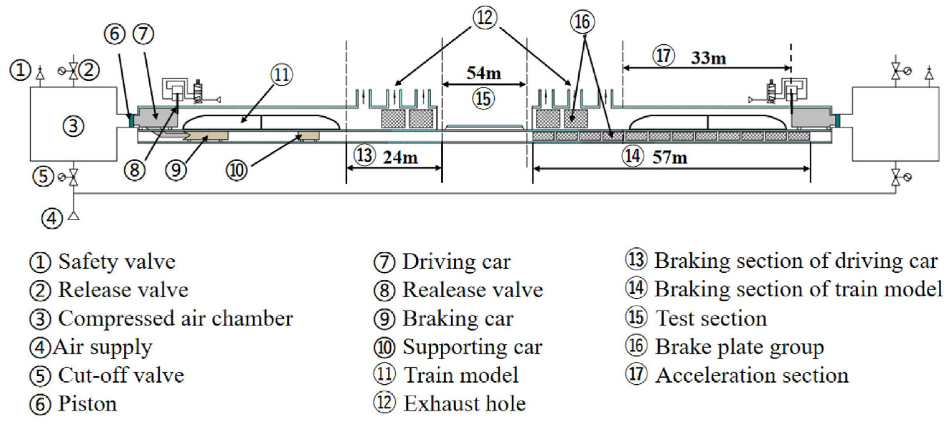
To validate the applicability and accuracy of the numerical methodology for simulating high-speed maglev trains traversing tunnels, computational results from the current study were compared against experimental data obtained from a 1:20 scaled moving model test conducted by [42] at the Key Laboratory of Traffic Safety on Track of the Ministry of Education (Central South University). The scaled test configuration, when converted to full-size dimensions, exhibits geometric consistency with the maglev train model employed in this study, including identical streamlined nose geometry and overall vehicle proportions. Figure 8 presents the detailed features of the model. The height of the train model (H) is 0.21 m, with the width and length equal to 0.88 H and 6.71 H, respectively, while the tunnel has a cross-sectional area of 0.35 m² and a total length of 75.86 H, and the experimental train speed is 600 km/h. In this study, monitoring point S2 on the tunnel wall surface was selected as a representative location for validating the numerical simulation methodology, where pressure data from this monitoring point was utilized for verification. The spatial positioning of monitoring point S2 is explicitly illustrated in Figure 5b.

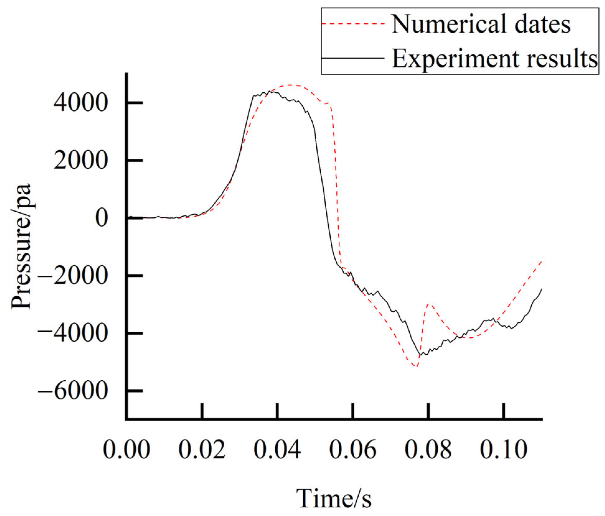
The mesh generation methodology, boundary conditions, and solver configurations employed in the numerical validation strictly align with those implemented in the present study. As demonstrated in Figure 9, which compares pressure variations at monitoring point S2 between the moving model experiment and numerical simulation results, the pressure evolution patterns exhibit fundamental consistency across both approaches. Observed discrepancies between experimental and numerical data may arise from geometric divergences in vehicle model implementations and uncertainties associated with boundary condition assumptions extrapolated from test conditions, such as the drag coefficients of the train and the tunnel and the consistency of air density, etc.

The accuracy of numerical simulation methods is typically evaluated through deviations in the positive/negative values and peak-to-peak amplitudes of monitoring point pressures. As evidenced by the comparative data presented in

Table 2. Evaluation of the accuracy of numerical modelling methods.

Pressure Sensor	Index	Experiment (kPa)	Simulation (kPa)	Deviation (%)
S2	${\mathrm{P}}_{\mathrm{m}\mathrm{a}\mathrm{x}\mathrm{i}\mathrm{m}\mathrm{u}\mathrm{m}}$	4.39	4.62	4.9
	${\mathrm{P}}_{\mathrm{m}\mathrm{i}\mathrm{n}\mathrm{i}\mathrm{m}\mathrm{u}\mathrm{m}}$	−4.78	−5.06	5.5
	peak-peak pressure	9.17	9.68	5.3

, the maximum deviation of evaluation metrics remains within 6%, thereby confirming that the numerical simulation results satisfy the precision requirements of this study.

4. Results and Discussions

The operating conditions investigated in this section are presented in

Table 3. Cases setup.

Case	Variables	Crosswind (√/✕)	Speed (m/s)	Crosswind Direction (Perpendicular to the Tunnel Axis)	Section
A1	—	✕	—	—	Section 4.1
A2	Wind Direction	√	30	Toward near-wall (left side)	Section 4.2
A3		√	30	Toward far-wall (right side)
B1	Wind Speed	√	5	Toward far-wall (right side)	Section 4.3
B2		√	10	Toward far-wall (right side)
B3		√	15	Toward far-wall (right side)
B4		√	20	Toward far-wall (right side)
B5		√	25	Toward far-wall (right side)
B6		√	30	Toward far-wall (right side)

. In Case A1, no crosswind was applied at the tunnel entrance. As the train enters the bidirectional tunnel, it travels along only one side of the tunnel. However, when a crosswind perpendicular to the tunnel exists at the tunnel entrance, the distributions of the flow field and pressure field exhibit significant asymmetry. Therefore, Cases A2 and A3 were established to comparatively analyze the influence of crosswind direction (perpendicular to the tunnel axis) on the aerodynamic effects of a high-speed maglev train entering the tunnel. When the maglev train operates under crosswinds of varying speeds, the aerodynamic pressure on its surface varies across different vehicles and heights, leading to the aerodynamic loads of the train being affected by the crosswind speed. The standard QX/T 334-2016 [43]. Levels of Severe Weather Impacting High-Speed Railway Operations categorizes multiple wind intensity levels affecting high-speed railway operations, with adjacent levels differing by an average wind speed v- of 5 m/s. Accordingly, Cases B1–B6 were designed to examine the influence of wind speed on the train.

In this study, the train velocity v was set to 600 km/h. The train entered the tunnel at t = 0.6 s, and the simulation was terminated at t = 2.1 s, by which time the train had fully penetrated 170 m into the tunnel. At this stage, the flow field within the tunnel and the aerodynamic loads on the train were deemed to have reached a steady state. For analytical convenience, the aerodynamic loads during the motion of the train are typically nondimensionalized.

4.1. Crosswind-Free Conditions

4.1.1. Aerodynamic Lift

The aerodynamic lift is defined with the vertical upward direction as positive. The aerodynamic lift coefficient ($C_L$) is expressed as follows (7). In the formula, $S_l$ is the aerodynamic lift reference area, specifically defined as the vertical projection area of the train, and the reference velocity v corresponds to the train’s running speed.

$$C_L={\displaystyle \frac{F_l}{0.5\rho S_l{v}^2}}$$

(7)

The HV, MV, and RV tunnel entry procedures are represented by the three phases in Figure 10a. Variations in the lift coefficient clearly reflect the aerodynamic characteristics of each vehicle during tunnel entry, as seen in the figure. The lift coefficient of the HV fluctuated slightly before tunnel entry (t < 0.60 s), remaining at approximately 0.002. Following tunnel entry, there were a few minor oscillations until they stabilized at zero, showing that any temporary aerodynamic disruptions in the tunnel environment had completely dissipated.

The dynamic behavior of the MV differed before tunnel entry (t < 0.77 s): its lift coefficient progressively decreased from 0.02 and eventually decayed to zero after tunnel entry, suggesting that its diminishing positive pitching trend stabilized fully within the tunnel.

In contrast, the aerodynamic interactions of the RV were more complex. Prior to tunnel entry (t < 0.93 s), the lift coefficient of the vehicles that came before them showed notable oscillations between 0.015 and 0.039, continuously moving upward and producing a dangerous alternating increase and drop tendency, which resulted in noticeable bumping risks. During tunnel traversal, this erratic pattern changed into a residual trend with slight oscillations (0.93 s < t < 1.09 s). Ultimately, the lift coefficient decayed to 0.02 after tunnel entry (t > 1.09 s), while the RV maintained a sustained positive pitching trend, markedly distinct from the fully stabilized HV and RV.

Throughout the tunnel traversal, the persistent lift coefficient of 0.02 for the RV created differential aerodynamic loads along the length of the train, exacerbating vertical instability and amplifying the risk of hazardous incidents compared to other sections. This analysis highlights the particularly adverse aerodynamic behavior of the RV during tunnel traversal, necessitating prioritized safety measures such as track contact prevention and operational stability enhancements.

4.1.2. Aerodynamic Lateral Force

The aerodynamic lateral force is defined as positive in the direction from the train toward the track center line. The aerodynamic lateral force coefficient ($C_S$) is defined as follows (8). In the formula, $S_s$ is the aerodynamic side force reference area, specifically defined as the lateral projection area of the train, and the reference velocity v corresponds to the train’s running speed.

$$C_S={\displaystyle \frac{F_s}{0.5\rho S_s{v}^2}}$$

(8)

Compared to aerodynamic lift, the aerodynamic lateral force change during train entry into tunnels exhibits more complexity. These lateral force fluctuations are primarily caused by the rapid evolution of asymmetric pressure distributions between the near-wall and far-wall sides of the train during the tunnel entry process under crosswind conditions. As shown in Figure 10b, prior to tunnel entry (t < 0.60 s), the HV exhibits initial lateral force fluctuations ranging from −0.0037 to 0.0066 (magnitude variation: 0.0103), accompanied by rapid directional reversal. This phenomenon indicates elevated derailment risks during the pre-tunnel entry phase. In comparison to the pre-entry stage, the lateral force coefficient of the HV exhibits a smaller oscillation amplitude as the vehicle passes through the tunnel (0.60 s < t < 0.77 s), retaining a constant upward vertical orientation. The lateral force experiences a sudden directional inversion from far-wall to near-wall orientation after full tunnel penetration (t > 0.77 s). This directional inversion is accompanied by a significant magnitude transition (peak values shifting from 0.0077 to −0.0074, total fluctuation range 0.0151), which causes abrupt lateral displacement tendencies during tunnel traversal. The HV is identified as a crucial zone for possible track deviation incidents due to its dual-phase instability pattern, which is characterized by lateral force reversal during both the pre-entry and intra-tunnel phases.

During the pre-entry period (t < 0.77 s), the MV exhibits significant derailment concerns, which show up as a lateral force inversion from 0.0060 to −0.0048. The near-wall directional component causes lateral displacement tendencies at the initial stage of entering the tunnel (t = 0.77 s), but this instability gradually lessens as the tunnel is traversed. Lateral forces exhibit oscillatory dampening until aerodynamic stabilization during the post-penetration period (t > 0.77 s).

The lateral force variation in the RV is also manifest in the stage before entering the tunnel. (t < 0.93 s). The RV experiences compounded aerodynamic effects from preceding vehicles, exhibiting initial lateral force escalation (peak 0.002) followed by precipitous decline to −0.0047 and gradual stabilization at −0.0016. This complex fluctuation profile indicates hazardous lateral force transients near tunnel portals correlating with high derailment probabilities. Subsequent operation maintains stabilized lateral force coefficient at −0.0016, suggesting sustained near-wall displacement tendency despite overall dynamic stability.

Comparative analysis reveals that all train segments experience significant lateral force coefficient transients in both magnitude and direction during pre-entry phases, constituting high-risk derailment conditions. Notably, lateral force coefficients in the HV demonstrate abrupt reductions coinciding with MV and RV tunnel entries, particularly showing directional mutation during RV penetration—a critical factor exacerbating derailment potential. During full tunnel operation (t > 1.09 s), MV and RV achieve aerodynamic stabilization with near-zero lateral forces, while the HV maintains persistent near-wall displacement tendency. This operational phase analysis confirms sustained lateral drift propensity at the train head during tunnel traversal, highlighting critical aerodynamic challenges in high-speed rail tunnel systems.

4.1.3. Overturning Moment

During tunnel entry, the combined aerodynamic action of lateral forces and lift induces an overturning moment on trains, with the overturning moment coefficient ($C_T$) defined as follows (9). In the formula, $S_t$ is the overturning moment reference area, which can be taken as the lateral projection area of the train, and the reference velocity v corresponds to the train’s running speed.

$$C_T={\displaystyle \frac{M_t}{0.5\rho S_t{v}^2}}$$

(9)

During tunnel traversal, all three train vehicles demonstrate distinct operational characteristics in their overturning moment coefficients. Prior to tunnel entry, each vehicle maintains coefficients slightly above zero but exhibits differentiated risk profiles in terms of peak magnitude, temporal evolution, and persistence of the overturning moment during tunnel penetration. After tunnel entry (t > 0.60 s), the HV experiences a sharp decrease in coefficient to about −0.0077; this sudden change in direction and magnitude suggests increased rollover risks during transitional periods. Concurrently, the MV displays a characteristic dip-recovery pattern, descending to −0.0032 during the pre-entry phase (t < 0.77 s) before stabilizing near neutral levels during tunnel operation. The RV manifests complex dynamics pre-entry (t < 0.93 s), particularly during HV penetration, where its coefficient plummets from 0.0034 to −0.0047, corresponding to critical rollover risk escalation. Post-entry stabilization occurs at 0.0011 after minor oscillations.

Based on extreme-value analysis of peak times, comparative analysis shows a consistent risk hierarchy during entry transitions: HV > RV > MV. While other vehicles return to safer operational states, the HV maintains a persistent overturning moment of −0.0077 throughout prolonged tunnel operation (t > 1.09 s), suggesting lingering rollover susceptibility at the train head.

4.2. Effect of Crosswind Directions

4.2.1. Effect of Crosswind Directions on Aerodynamic Lift of Trains

Aerodynamic lift coefficient time-history graphs for several train sections under operational cases A2 and A3 are shown in Figure 11a Comparative analysis with Figure 10a reveals that crosswind-influenced lift coefficient profiles maintain dynamic similarities to crosswind-free conditions during tunnel traversal. Specifically, all vehicles show a pattern consistent with baseline crosswind-free operations: sudden lift reduction during tunnel penetration followed by stabilization post-entry. Notably, crosswind effects elevate lift coefficients across all vehicles compared to the crosswind-free baseline. During HV and MV tunnel entries, RV retain higher lift magnitudes than crosswind-free conditions while avoiding their characteristic fluctuations, indicating that crosswind effects substantially modify the pressure distribution patterns over train surfaces.

Figure 11a demonstrates that identical train vehicles generate consistently higher lift values under Case A2 compared to Case A3. All vehicles experienced a significant drop in lift coefficient when entering the tunnel under the influence of crosswinds: 0.084 (HV), 0.063 (MV), and 0.045 (RV) in A2 compared to 0.069, 0.049, and 0.025 in A3, respectively. This behavior suggests enhanced oscillation risks and potential derailment hazards during tunnel entry transitions, with Case A2 presenting greater risks than A3. Both cases exhibit front-to-rear risk gradation: HV> MV > RV. During stabilized tunnel operation, lift coefficients converge to identical levels in both cases, confirming that sustained crosswind forces pose negligible hazards to fully immersed trains.

4.2.2. Effect of Crosswind Directions on Aerodynamic Lateral Force of Train

Figure 11b illustrates the time-history curves of aerodynamic lateral force coefficients across train sections under Cases A2 and A3. Comparative analysis with Figure 10b reveals distinct pre-tunnel-entry aerodynamic characteristics under crosswind conditions compared to crosswind-free conditions. The HV and MV exhibit elevated lateral force coefficients with sustained minor oscillations, contrasting sharply with the abrupt directional reversals observed in crosswind-free cases, while the RV demonstrates intensified pre-entry fluctuations of prolonged duration. During tunnel penetration, all sections experience rapid lateral force attenuation followed by stabilization near equilibrium states approaching zero, a dynamic response pattern consistent with crosswind-free conditions.

Due to the opposite crosswind directions in Cases A2 and A3, applying the positive direction defined in Section 4.1.2 would naturally assign opposite signs (one positive and one negative) to the lateral forces of opposite physical directions acting on the same part of the train at the same moment. This difference in sign would cause the graphical curves of the lateral force coefficients for the two cases to exhibit a near “mirror-image” symmetry, thereby making the representation of both the magnitude and abrupt changes in the lateral forces highly unintuitive. For analytical clarity, in Case A3 (inverse to Case A2), the positive lateral force is defined as acting from the track center line toward the train in order to eliminate directional effects. The findings show that, in crosswind conditions, Case A2 produces noticeably greater aerodynamic lateral force coefficients than Case A3, with gradient-distributed differences across train sections. In particular, under A2, the average lateral force coefficients for the head, middle, and rear portions during open-air operation are 0.105, 0.018, and −0.012, respectively, while under A3, they are 0.083, 0.015, and −0.011, respectively. During open-track operation, this pattern creates destabilizing yaw moments due to a combination of leeward-directed forces on the HV and MV and windward-directed forces on the RV. The HV experiences critical lateral force reversals during crosswind-influenced tunnel entry: its coefficient drops from 0.12 to −0.0039 (Δ0.1239) in A2 and from 0.083 to −0.0023 (Δ0.0853) in A3, indicating sudden aerodynamic changes in magnitude and direction at tunnel portals that increase the risk of derailment, especially under A2.

Concurrently, Case A3 triggers hazardous directional inversion in the RV, with lateral force rising from −0.001 to 0.005 during entry, while the MV maintains transitional stability. Post-entry stabilization phases exhibit consistent lateral force magnitudes and directions across all sections, ensuring operational safety. With transitional risk prioritizing based on a front-to-rear hierarchy (HV > RV > MV), which is compatible with aerodynamic load redistribution methods in crosswind-tunnel interactions, comparative analysis validates the increased risk severity of Case A2 due to larger force fluctuation amplitudes.

4.2.3. Effect of Crosswind Directions on Overturning Moment of Trains

Figure 11c presents the time-history curves of overturning moment coefficients across train sections under Cases A2 and A3. Comparative analysis with Figure 10c indicates that overturning moments under crosswind conditions exhibit trends similar to those observed in crosswind-free operations. Notably, the HV demonstrates a significant increase in pre-tunnel-entry peak overturning moments compared to crosswind-free conditions, while all three vehicles stabilize post-entry to levels consistent with crosswind-free conditions.

During open-track operation, Case A2 exhibits substantially higher rollover risks for the HV, with average coefficients of 0.073 versus 0.047 in A3. This disparity stems from the aerodynamic lateral force dominating overturning moment generation due to its larger horizontal distance to the load application point compared to aerodynamic lift effects. This occurrence emphasizes the critical connection between the overturning moment and the lateral force dynamics, particularly in situations with a strong crosswind, such as case A2, when the horizontal distance of the load application point is tiny. During tunnel entry, the abrupt attenuation of lateral forces triggers sudden overturning moment transitions, corresponding to peak rollover risks. Open-track operation maintains minimal rollover risks for MV and RV in both cases, with coefficients below 0.01, further decreasing to near-neutral stability at tunnel portals. Comparative analysis confirms the HV bears the highest rollover risk during tunnel entry transitions, while MV and RV achieve rapid stabilization.

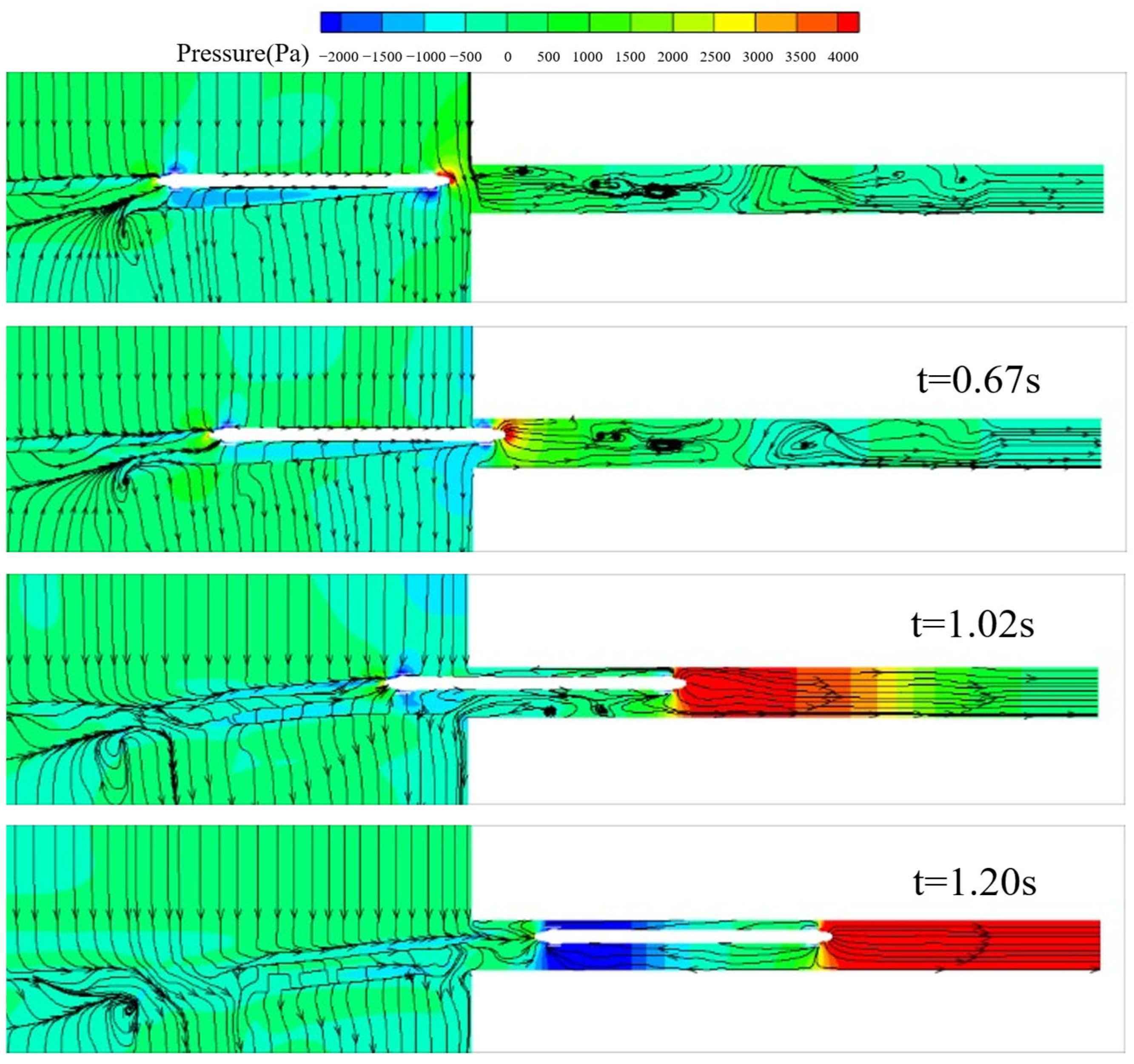
Analysis and discussion of the aerodynamic pressure field and flow distribution around the train under the most critical A2 case:

Figure 12 presents instantaneous pressure contours combined with streamlines on a representative longitudinal mid-plane passing through the train centerline, which is used to qualitatively examine the pressure field and flow organization during tunnel entry under crosswind conditions. Prior to tunnel entry, a pronounced asymmetric pressure distribution is observed on the lateral surfaces of the maglev train, with the positive pressure region on the windward side of the head HV shifting toward the crosswind direction, while the leeward side remains dominated by negative pressure. This pressure imbalance between the two sides of the train constitutes the primary aerodynamic mechanism driving lateral force and overturning moment generation, thereby explaining the elevated rollover risk of the HV in the pre-entry phase.

As the train penetrates into the tunnel, the lateral pressure asymmetry gradually weakens, and the pressure distribution on both sides of the train tends toward a more symmetric pattern, resulting in reduced crosswind influence within the tunnel. During the pre-entry stage, the interaction between the incoming crosswind and the train-induced flow generates multiple vortical structures near the tunnel portal, which persist dynamically until the train fully enters the tunnel. Once the train has fully entered the tunnel, a relatively stable train-induced flow field is established inside the tunnel, indicating that the influence of crosswind on the internal tunnel flow is mainly confined to the entry process.

The visualization demonstrates that during crosswind-influenced tunnel entry of the maglev train, the flared nose geometry of the TV induces prominent separation vortices on its leeward rear side. These vortices may generate aerodynamic interference with opposing trains, necessitating further systematic investigation into crosswind encounter dynamics of maglev systems.

4.3. Effect of Crosswind Speed

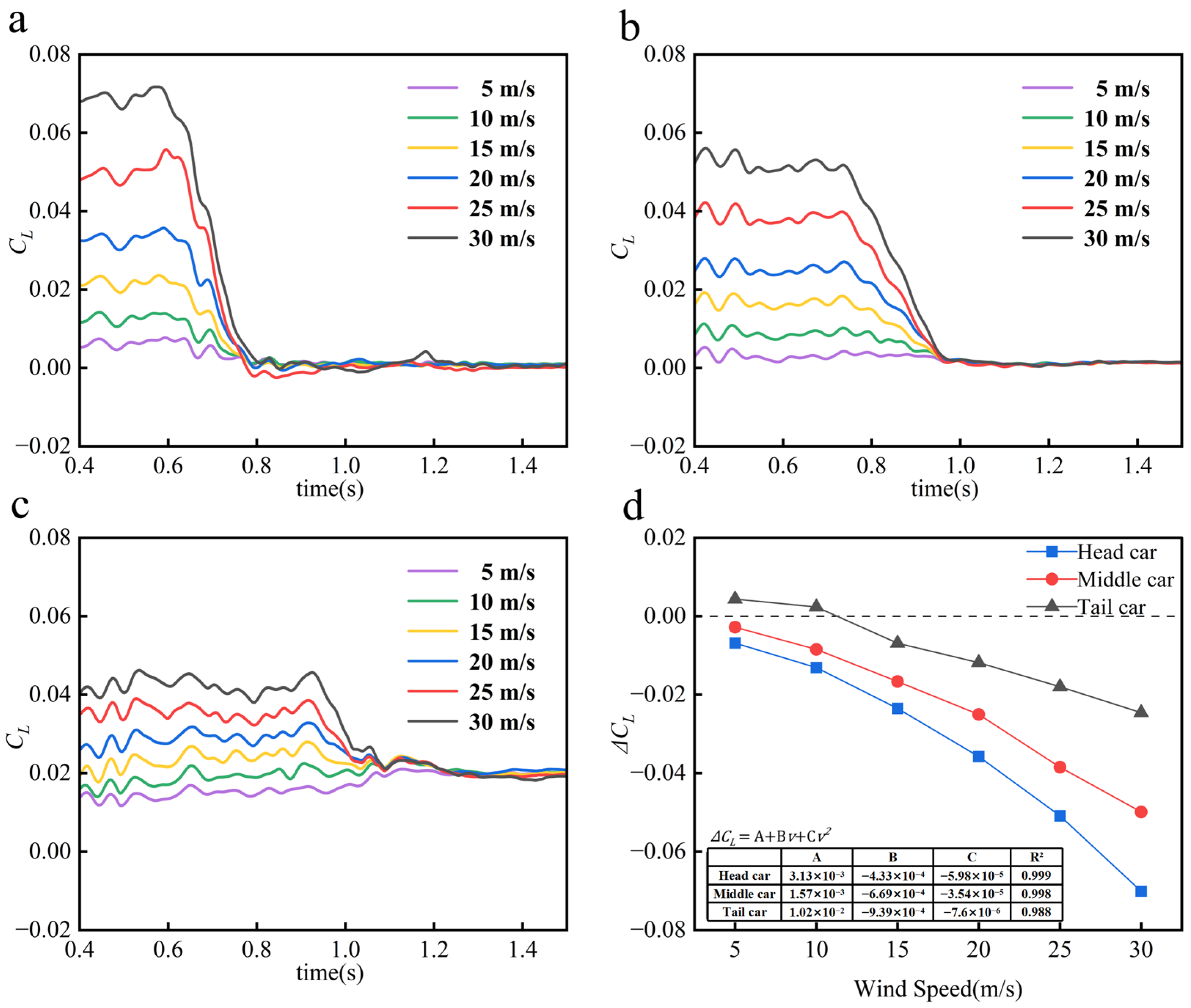
4.3.1. Effect of Crosswind Speed on Aerodynamic Lift of Train

Figure 13a–c demonstrates that prior to tunnel entry, all train vehicles exhibit positive aerodynamic lift coefficients in the vertically upward direction, with magnitudes positively correlated to crosswind speed. During tunnel traversal, abrupt variations in lift coefficients occur across vehicles: the HV and MV show significant reductions, while the RV displays divergent trends—lift enhancement at crosswind speeds below 10 m/s but attenuation at speeds exceeding 15 m/s. Figure 13d quantifies the magnitude of lift coefficient variations during tunnel entry under varying crosswind speeds. The differences in variation magnitudes amongst vehicles gradually expand as crosswind intensity increases, with the HV seeing the most noticeable crosswind-dependent lift fluctuations, followed by the MV and RV. This pattern confirms that the HV faces the highest vertical oscillation risks during crosswind-influenced tunnel entry, exhibiting heightened sensitivity to crosswind speed variations in vertical stability. The effect of crosswind speed on aerodynamic lift coefficients quickly decreases in all portions after entry. Regardless of the initial strength of the crosswind, lift coefficients stabilize and converge toward homogeneity as the train moves farther into the tunnel.

4.3.2. Effect of Crosswind Speed on Aerodynamic Lateral Force of Trains

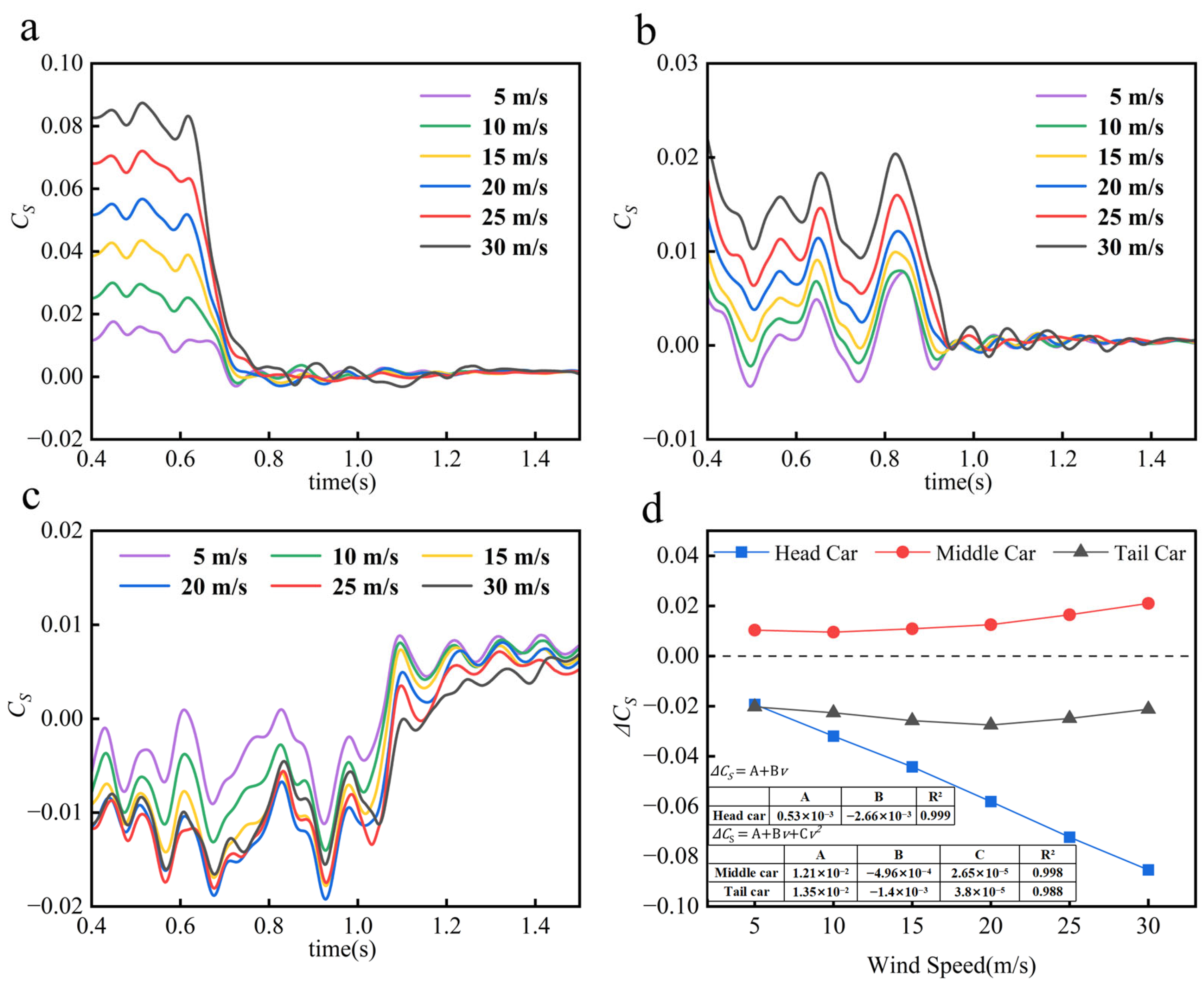
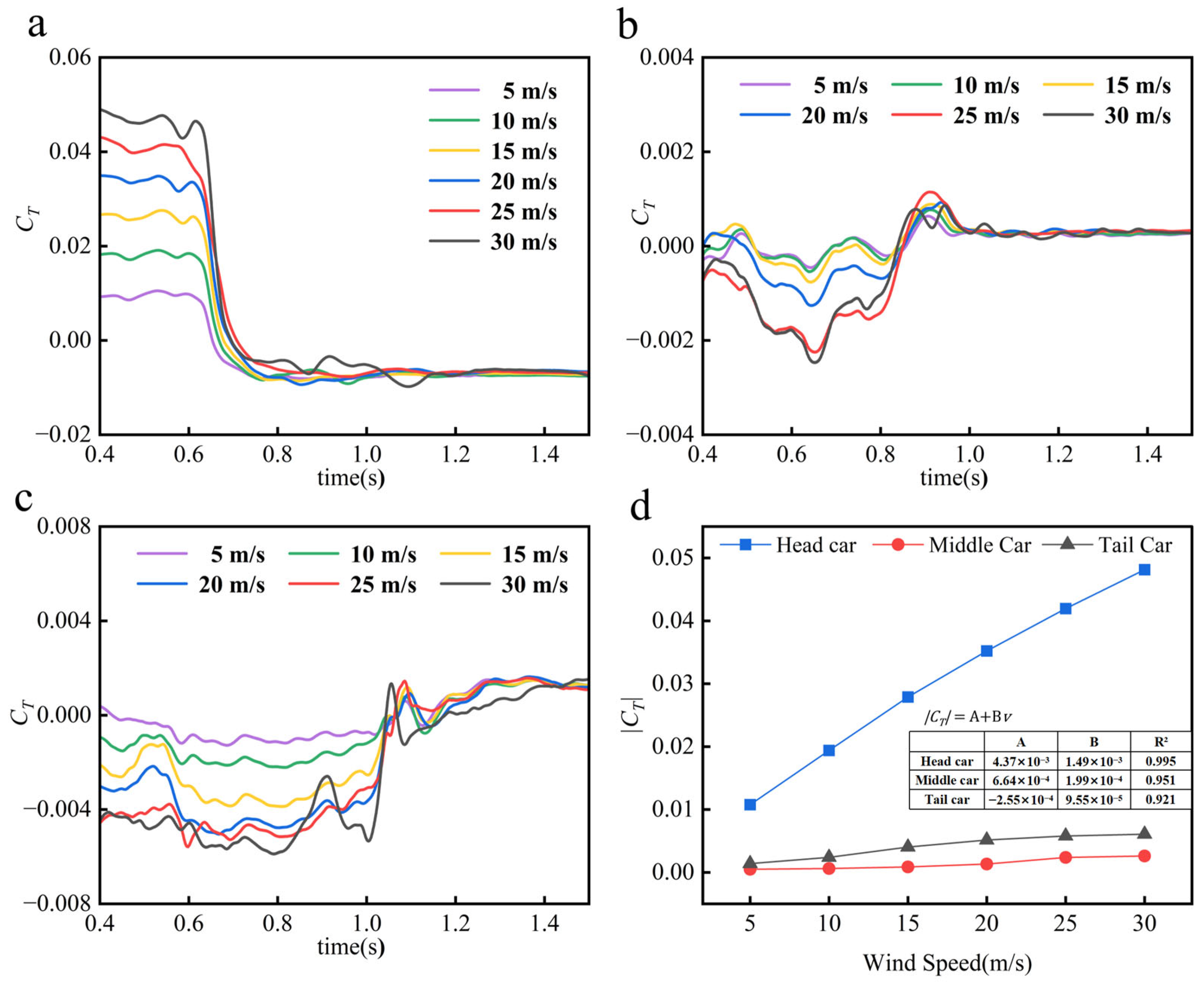
Figure 14 reveals that during tunnel entry, all train vehicles undergo rapid variations in aerodynamic lateral force magnitudes, with directional inversions occurring in all three sections under specific crosswind speeds, as detailed in

Table 4. Peak values of $C_S$ before and after mutation at different crosswind velocities (10⁻³).

Speed (m/s)	5		10		15		20		25		30
	Max	Min	Max	Min	Max	Min	Max	Min	Max	Min	Max	Min
HV	16.2	−3.1	29.8	−2.2	43.8	−0.4	57.1	−1.0	72.4	0.2	87.8	2.5
MV	7.8	−2.5	8.0	−1.5	10.1	−0.8	12.2	−0.3	16.1	−0.3	20.6	−0.4
RV	8.9	−11.4	8.4	−14.2	7.8	−18.0	8.2	−19.4	7.2	−17.7	5.3	−15.8

. During entry, the HV undergoes sudden decreases in the lateral force coefficient, and the amplitude attenuation increases linearly with wind speed. In contrast, the MV exhibits progressive lateral force amplification during penetration, its amplitude growth rate positively correlated with crosswind intensity. For the RV, lateral force coefficients decline during entry, showing reductions comparable to the HV at 5 m/s crosswind. But as wind speeds increase, this attenuation becomes slightly stronger, reaching a peak at 20 m/s before progressively decreasing. Comparative analysis confirms the HV exhibits the most pronounced lateral force fluctuations, demonstrating higher sensitivity to wind speed variations than MV and RV. It is noteworthy that the fitting analysis reveals a linear increase in the amplitude attenuation of the lateral force coefficient for the HV with wind speed. As shown in Figure 14d, the linear relationship exhibits an excellent goodness of fit (R² = 0.999), confirming a robust linear dependence between the two variables.

Table 4 shows a unique phenomenon: under extreme wind speeds (25–30 m/s), the HV maintains directional consistency in lateral forces despite significant magnitude variations, whereas directional and magnitude reversals co-occur under other operational conditions. The findings point to a complex and nonlinear link between lateral stability during tunnel entry and crosswind intensity. Given that both force magnitude and directional changes contribute to derailment risks, the impact of crosswind speeds on maglev train lateral stability during tunnel entry defies generalized patterns, necessitating further targeted investigations to elucidate scenario-specific dynamics.

4.3.3. Effect of Crosswind Speed on Overturning Moment of Train

Figure 15a–c demonstrate that prior to tunnel entry, the HV maintains positive overturning moment coefficients across all wind speed conditions, with magnitudes increasing proportionally to wind speed. During tunnel penetration, overturning moment coefficients under varying crosswind intensities plummet abruptly before stabilizing at approximately −0.0063. The MV and RV exhibit significant pre-entry overturning moment fluctuations positively correlated with wind speed, though with lower fluctuation amplitudes compared to the HV, followed by gradual stabilization post-entry.

Figure 15d illustrates extreme values of overturning moment coefficients during tunnel entry under different crosswind speeds. Absolute values of positive and negative peaks were analyzed to eliminate directional effects, with the larger magnitude selected for comparison. Analysis of dominant peaks reveals a consistent positive correlation between wind speed and peak magnitudes across all train sections. The HV exhibits the highest sensitivity to wind speed variations, followed by the RV, with the MV showing slightly lower sensitivity than the RV. This head-rear disparity in wind speed sensitivity highlights the uneven distribution of rollover risks along the longitudinal axis of the train during tunnel entry, underscoring the heightened susceptibility of the HV to crosswind-induced instabilities at tunnel portals.

4.4. The Mitigating Effect of Running Speed

To investigate the mitigation effect of speed reduction on the crosswind response of high-speed maglev trains in tunnels, this subsection conducts numerical simulations under five operating conditions, denoted as C1 to C5. In Condition C1, the train operates at a speed of 600 km/h. For Conditions C2 to C5, the train speed is reduced by 50 to 200 km/h, respectively, while all other parameters remain consistent with those described in Section 4.3. Detailed settings for these conditions are provided in

Table 5. Working condition settings for different train operating speeds.

Case	C1	C2	C3	C4	C5
Speed (km/h)	600	550	500	450	400

.

Based on the conclusions from Section 4.2 and Section 4.3, during the process of a maglev train entering a tunnel under crosswind conditions, the head car exhibits greater variations in lift coefficient and lateral force coefficient, as well as a higher peak overturning moment coefficient, compared to the middle and tail cars. Therefore, in this subsection, the head car is selected as the most critical car for analysis, to investigate the effects of operating speed on the aerodynamic lift, lateral force, and overturning moment.

By applying the aforementioned aerodynamic load coefficients, this study evaluates the effectiveness of speed reduction operation in mitigating the aerodynamic characteristics of a maglev train during tunnel entry. Based on simulation data, fitting curves establishing relationships between operational speed and four parameters, namely the reduction amplitudes of aerodynamic lift and lateral force coefficients during head car tunnel entry, along with the maximum overturning moment coefficients for the head car operating in both open air and tunnel environments, are presented in

Table 6. Fitting results of relation between pneumatic load factor and train speed. Aerodynamic coefficients C*, representing the lift ($C_L$), lateral force ($C_S$), and overturning moment ($C_T$) coefficients.

Coefficient Indicator C*		C* = A + BV + CV2
		A	B	C	R2
$\mathrm{Amplitude} \mathrm{of} C_L$		4.80 × 10−2	8.31 × 10−6	5.43 × 10−8	0.98794
$\mathrm{Amplitude} \mathrm{of} C_S$		4.48 × 10−3	1.53 × 10−4	−1.50 × 10−8	0.98507
$\mathrm{Extreme} \mathrm{value} \mathrm{of} C_T$	open air	−9.91 × 10−3	1.06 × 10−4	1.73 × 10−9	0.99083
	tunnel	2.58 × 10−3	−4.93 × 10−6	2.93 × 10−8	0.99606

. Analysis indicates that for every 50 km/h reduction in train speed, the four aerodynamic load coefficients documented in Table 6 decrease by approximately 4.8%, 8.9%, 11.4%, and 15.7%, respectively.

4.5. Discussion

The aerodynamic load characteristics of maglev trains inside tunnels share similarities with those of wheel-rail trains but also exhibit notable differences. In the absence of crosswinds, the variation trends of aerodynamic loads are generally consistent with the findings of Wang et al. [5] though the magnitudes of variation are more pronounced due to the significantly higher speeds. Under crosswind conditions, the aerodynamic load coefficients of the three-carriage train fluctuate more intensely as wind speed increases. Meanwhile, the HV experiences the most significant impact on aerodynamic lift, lateral force, and overturning moment, resulting in a higher risk of derailment and overturning compared to the MV and RV.

A comparative analysis of scenarios with and without crosswind reveals that under crosswind-free conditions, HV and RV exhibit the worst overturning moment and lift characteristics, respectively, which results in the highest risks of overturning and collision. Additionally, all three vehicles demonstrate certain derailment risks. When crosswind is present, the HV shows the highest sensitivity and risk to all three types of aerodynamic loads. Consequently, under crosswind influence, the risk profile shifts from being distributed across the three vehicles, each with its specific safety concerns, to one where the HV simultaneously carries the highest safety risks of collision, derailment, and overturning.

The amplitude of the lateral force on the HV exhibits an approximately linear relationship with wind speed and maintains a consistent direction under extreme wind conditions. To mitigate potential hazards, reducing the operating speed of the train can alleviate these effects. It is also observed that the amplitude of the aerodynamic load coefficients roughly follows a quadratic relationship with train speed. Furthermore, when a maglev train enters a tunnel under crosswind, the flared nose geometry of the RV induces prominent separation vortices on its leeward rear side, which may interfere with the operation of opposing trains. These findings address a research gap regarding maglev trains entering tunnels under crosswind conditions and provide theoretical support for enhancing the operational safety of maglev systems.

5. Conclusions

This study employs the FLUNET computational fluid dynamics software to conduct numerical simulations of aerodynamic effects on high-speed maglev trains entering tunnels under crosswind conditions. The principal conclusions can be summarized as follows:

• When a high-speed maglev train enters a tunnel under crosswind-free conditions, the RV exhibits the most severe lift characteristics, experiencing greater vertical oscillations and higher risks of track contact incidents compared to the HV and MV; the HV demonstrates the maximum overturning moment, representing the highest overturning risk; all three vehicles undergo abrupt transitions in lateral force coefficients immediately before tunnel entry, simultaneously facing elevated derailment risks.
• When the train enters the tunnel, the airflow over its surface becomes turbulent, leading to a significant abrupt change in the aerodynamic torques on all three vehicles, which then stabilizes after the train fully enters the tunnel. Crosswinds further increase the aerodynamic torques on the train surface. The increase in torques is significantly higher when the crosswind comes from the near-wall region of the tunnel compared to the far-wall region condition, and this torque intensifies with rising wind speed.
• When a maglev train enters a tunnel under crosswind conditions, the aerodynamic lift, lateral forces, and overturning moment acting on all three vehicles exhibit proportional relationships with crosswind speed. The aerodynamic loads on the HV demonstrate far greater sensitivity to crosswind speed variations than those on the MV and RV, with the lateral force displaying the strongest speed dependence. Specifically, the amplitude reduction magnitude in the lateral force of the HV exhibits a nearly linear progression with increasing wind speed.
• A distinctive phenomenon has been discovered: under extreme wind speeds (25–30 m/s), the HV maintains directional consistency in lateral forces despite significant magnitude variations, whereas under other operational conditions, directional and magnitude reversals occur simultaneously.
• When a maglev train enters a tunnel at different operating speeds, a reduction in speed by 50 km/h results in decreases of approximately 4.8%, 8.9%, 11.4%, and 15.7%, respectively, in the amplitude of change for the lift coefficient, the lateral force coefficient, and the peak overturning moment measured in both open air and inside the tunnel.

This study investigates the aerodynamic effects of high-speed maglev trains entering tunnels under crosswind conditions, yet certain limitations merit further in-depth exploration:

• Future studies may further investigate detailed flow-field characteristics during tunnel entry under crosswind conditions, including turbulence structures and turbulent stress distributions. In addition, thermodynamic effects such as temperature variations along the train surface and associated air property non-uniformities could be incorporated to provide a more comprehensive understanding of the underlying flow physics.
• The variability of gravitational acceleration associated with geographical location and tidal effects represents a potential research direction, particularly regarding its influence on gravity-driven ambient airflow, including the mean slip velocity and velocity profiles around high-speed trains. Accounting for such variability may improve the physical fidelity of aerodynamic analyses under realistic environmental conditions.