A Matrix-Statistics-Aware Attention Mechanism for Robust RUL Estimation in Aero-Engines

Abstract

Prognostics and Health Management (PHM) is a vital approach which aims to predict the failure of engineering systems at an early stage and optimize maintenance strategies. It operates through continuous system monitoring, anomaly detection, fault detection, and Remaining Useful Life (RUL) estimation. Accurate RUL prediction for aircraft engines is critical for enhancing operational safety and minimizing maintenance costs. Traditional methods are largely dependent on handcrafted features and domain-specific knowledge. They often fail to capture the nonlinear and high-dimensional degradation dynamics of real-world systems. In this study, we propose an enhanced deep learning architecture combining Long Short-Term Memory (LSTM) and Bidirectional LSTM networks with a new Matrix-Statistics-Aware Attention (LSTM-MSAA) method. Unlike conventional attention methods, our proposed method incorporates auxiliary scalar features, such as the Frobenius norm, spectral norm, and soft rank, into the attention score computation. This hybrid model provides a more informative representation of engine state transitions. The model is evaluated on both legacy and newly released C-MAPSS datasets from NASA’s Prognostics Data Repository. Experimental results reveal a reduction in RMSE compared to baseline models, validating the effectiveness of our attention fusion strategy in capturing intricate degradation behaviors and improving predictive performance.

1. Introduction

Prognostics and Health Management (PHM) is an interdisciplinary field that integrates data-driven methodologies, physics-based models and domain expertise to ensure the reliability and operational continuity of critical systems [1,2,3]. PHM utilizes historical and real-time state information of systems and their subcomponents [3]. Ultimately, this facilitates the ability to make more informed decisions regarding maintenance, repair, and replacement. In the aviation industry, avionics, flight controls, fly-by-wire, engines, thrust reversers, landing gear, braking, environmental control systems, electrical systems, auxiliary power units, and other components can be monitored through sensors to ensure safety, reliability, maintainability, and performance [4].

PHM systems are analyzed under three main headings [2]: Fault Prediction, Anomaly Detection and Remaining Useful Life (RUL) Estimation.

There are four different approaches for PHM. These are experience-based, physics-based, data-driven, and hybrid versions [5]. Each approach has its advantages and drawbacks. Experience-based approaches require historical repair and failure data. Physics-based approaches require the use of mathematical models. A data-driven approach requires monitored and historical data to validate the prognostic performances against possible faults. The hybrid method combines several approaches into a single solution to make more accurate predictions [6]. Data-driven prognostics can be applied to components, subsystems, and system levels [7]. Statistical and machine learning approaches are the other classification types of data-driven PHM. This article presents an experimental study on the data-driven prognostics approach.

Data-driven approaches have shown superior capabilities for capturing non-linear patterns and temporal dependencies in engine degradation data. Among these methods, machine learning methods such as Support Vector Machines (SVM) and Random Forests, deep learning-based Convolutional Neural Networks (CNN), Long Short-Term Memory (LSTM), Bidirectional LSTM (BiLSTM), Attention Mechanisms and Transformer models stand out [8,9,10]. Attention mechanisms enable the model to focus on critical time or sensor points, filter out redundant information and learn long-term dependencies [11]. Attention mechanisms integrated with LSTM prioritize specific moments in time series, whereas CNN-based systems prioritize important sensor data [12]. Transformer models, on the other hand, analyze global relationships across both time and sensors with the self-attention mechanism [13]. These methods enable data-driven approaches to exhibit better generalization and prediction capabilities, especially under high-dimensional and complex conditions.

Despite the strong performance of attention-based and Transformer architectures, most existing methods learn temporal and cross-sensor dependencies in an implicit manner, which limits their interpretability and sensitivity to structural degradation patterns. Recent studies have attempted to address this limitation through graph-based and hypergraph-based models that explicitly encode sensor connectivity and higher-order interactions [14]. However, such approaches require predefined or learned graph structures, are sensitive to graph construction strategies, and often introduce significant computational overhead, restricting their scalability and applicability in real-time PHM scenarios.

In contrast, degradation processes in complex systems such as turbofan engines often manifest as changes in the global energy, dominant latent modes, and structural complexity of multivariate sensor windows. These characteristics are not fully exploited by similarity-based attention mechanisms. Motivated by this observation, this study proposes a Matrix-Statistics-Aware Attention (MSAA) mechanism that embeds matrix-level descriptors directly into the attention score computation, enabling the model to attend to structurally informative temporal segments without relying on explicit graph or hypergraph formulations.

These developments collectively indicate that advanced attention-driven architectures offer strong generalization and predictive capabilities under high-dimensional and heterogeneous operating conditions.

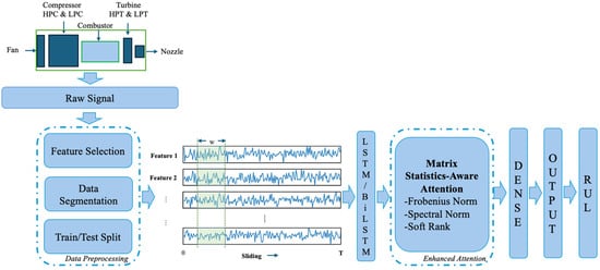
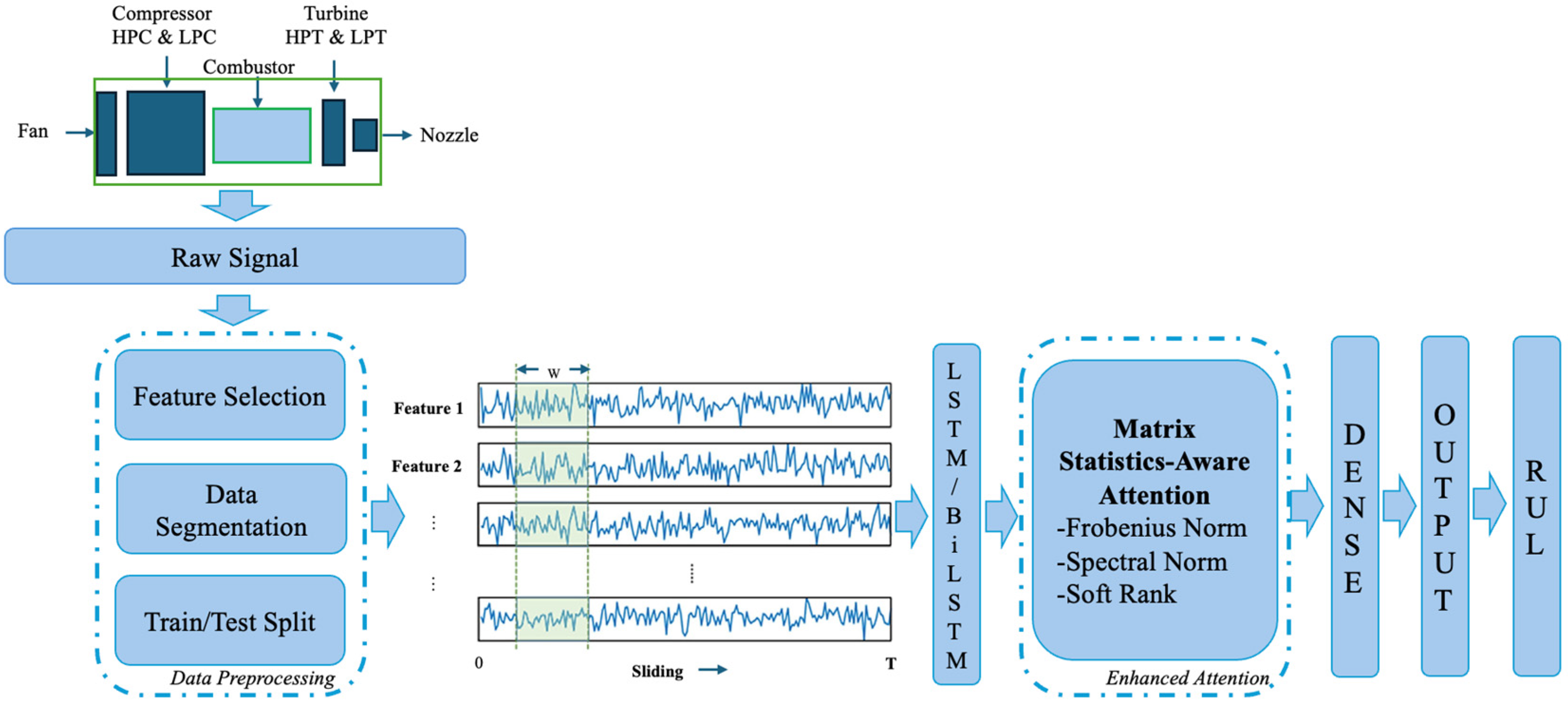
In this study, an LSTM model is combined with a MSAA mechanism to provide a model that improves RUL prediction performance in turbofan engines. The study utilized the old and new Commercial Modular Aero-Propulsion System Simulation (C-MAPSS & N-CMAPSS) turbofan engine data sets provided by the Prognostics Data Repository of NASA [15]. The system’s flowchart is presented in Figure 1.

Figure 1. System flowchart [16].

The main contributions of this study are listed below:

• This study introduces an LSTM-MSAA mechanism, in which scalar descriptors such as the Frobenius norm, spectral norm, and soft rank are embedded directly into the attention score calculation to extract deeper structural information from the input time series.
• The scaled dot-product attention score is enriched with three matrix-level descriptors, so the model MSAA can attend to segments that carry strong structural signals and complexity, not only similarity.
• Unlike prior norm or SVD-based attention formulations that focus on regularization or efficiency, the proposed MSAA leverages matrix statistics as degradation-aware contextual signals within the attention score itself.
• Two benchmark datasets, C-MAPSS and N-CMAPSS, are used to comprehensively validate the proposed approach, demonstrating its robustness across both legacy and modern turbofan engine scenarios.
• The model treats sliding windows as temporal matrices and leverages matrix-level descriptors to enhance the attention mechanism, offering a new perspective on how to prioritize input segments in prognostic tasks.
• The integrated attention mechanism with LSTM and BiLSTM architecture enables the model to capture both long-term temporal dependencies and localized matrix-structured features.
• Experimental results highlight that MSAA improves RMSE performance over conventional attention models, especially in handling nonlinear and nonstationary behaviors in engine health trajectories.
• The study offers a generalizable framework that can be extended to other complex systems where hidden structural signals within time series need to be emphasized through learned attention.

The structure of this paper is organized as follows: Section 2 covers the related work within the last five years, Section 3 gives information about datasets and details the framework of the proposed method, and Section 4 discusses the results. The paper concludes in Section 5, where key findings are summarized and future research opportunities are discussed.

2. Related Works

Turbofan Remaining Useful Life (RUL) prediction has been extensively studied using the C-MAPSS and, more recently, the N-CMAPSS datasets. Prior research over the past five years has predominantly adopted deep learning methods, reflecting the increasing complexity and scale of these datasets [17]. Attention-enhanced architectures have become particularly influential due to their ability to highlight critical temporal regions and improve long-term dependency modeling.

A broad line of studies integrates attention mechanisms with recurrent networks. Representation-learning approaches based on Variational Autoencoder (VAE) [18], hybrid attention-enhanced LSTM models such as Attention Long Short-Term Memory Projected (ALSTMP) [19] and Spatial Correlation and Temporal Attention-based LSTM (SCTA-LSTM) [20], and classical LSTM-Attention formulations [21,22,23] have demonstrated consistent improvements across C-MAPSS and N-CMAPSS. Additional enhancements include multiscale patching and local attention [24], stacked BiLSTM with scaled dot-product attention [25], and PCA-BiLSTM hybrids that reduce redundancy before sequence modeling [26]. While existing studies have extensively explored recurrent architectures and attention mechanisms for time-series modeling, the majority of these approaches formulate attention purely based on pairwise similarity or temporal alignment.

Beyond recurrent models, graph-based architectures such as Spatial-Temporal Dual-Channel Adaptive Graph Convolutional Network (SDAGCN) [27] and physics-informed formulations like Dynamic Governing Networks [28] further expand the design space for RUL prediction.

Most papers above have hybrid architectures that combine multiple modules and integrate attention to improve sequence modelling, enhancing focus on critical time steps (temporal) or features (spatial) on turbofan datasets.

Conventional attention mechanisms, including additive attention and scaled dot-product self-attention, assign importance weights based on pairwise similarities between temporal features or hidden states. While effective for highlighting locally relevant time steps or sensor channels, such mechanisms do not explicitly encode the global structural characteristics of the underlying time-series representation.

The following referenced works introduce innovations to the classical attention structure from different perspectives. They focused on advanced attention mechanisms and validated them on different datasets [29,30,31,32,33]. Relative positional encodings [29], the linear-complexity Linformer [30], and multi-branch temporal–channel attention in Mixformer [31] extend the expressive power of self-attention in time-series forecasting. Primal Attention [32] reframes attention through an asymmetric kernel Singular Value Decomposition (SVD) formulation, while subsequent SVD-based analyses [33] highlight the underlying role of matrix factorization in modern attention operators. LECformer [34] combines Transformer structures with Local Enhanced Channel Self-Attention (LECSA) to capture long-term dependencies and cross-sensor interactions on turbofan datasets. Overall, existing studies confirm the strong utility of attention-based architectures for RUL prediction. In degradation modeling, however, the evolution of failure is not only reflected in local temporal patterns but also in changes to the global structure of multivariate sensor trajectories. The proposed matrix-statistics-aware attention mechanism addresses this limitation by embedding matrix-level descriptors, which are Frobenius norm, spectral norm and soft rank, directly into the attention score computation. Although Frobenius norm has appeared in prior works, its role is fundamentally different. Existing studies primarily employ it as a regularization or distillation loss to align internal representations between models [35]. In ST-KDFormer, Frobenius and spectral matrix norms are used to regularize and validate the stability of learned Koopman operators in latent space [36]. To the best of our knowledge, prior C-MAPSS/N-CMAPSS RUL studies do not explicitly inject matrix-level soft-rank descriptors as input-dependent structural cues into the attention scoring. Existing uses of rank- or SVD-related operators in PHM and fault diagnosis literature primarily focus on regularization, computational efficiency or optimization tools for learning scalar-valued rank orderings [37,38].

In contrast, this work introduces these matrix-level descriptors as an input-dependent structural descriptor computed directly from multivariate sensor windows and embedded into the attention scoring mechanism, enabling degradation-aware attention rather than representation alignment. This matrix-statistics-aware formulation enriches the attention module with global structural cues and complements a dual-layer LSTM backbone for improved degradation modeling on C-MAPSS and N-CMAPSS.

3. Materials and Methods

3.1. Dataset

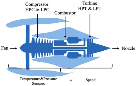
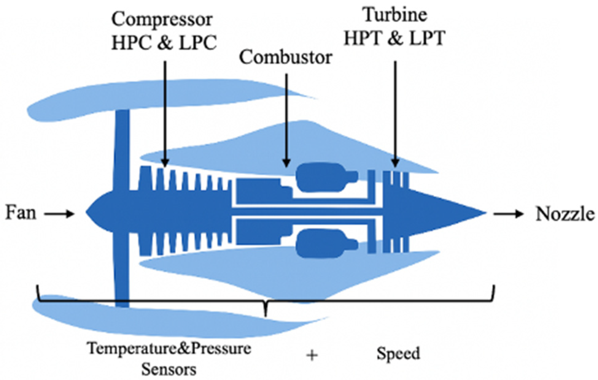
The C-MAPSS dataset, introduced by NASA in 2006, provides a simulation environment for modeling turbofan engine performance and degradation under varying operating conditions and has become a widely used benchmark for data-driven RUL prediction [16]. Its extended successor, N-CMAPSS, released in 2020, offers a richer representation of modern engine behavior by incorporating multiple operating modes and more detailed degradation scenarios [39]. Together, these two simulation models serve as the primary data sources for PHM research. A schematic overview of the C-MAPSS framework is presented in Figure 2.

Figure 2. Schematic representation of the C-MAPSS model [16].

3.1.1. C-MAPSS Dataset

The C-MAPSS dataset is a widely recognized benchmark in the PHM community, particularly for RUL prediction in aircraft engines [40]. The NASA turbofan engine dataset was developed using MATLAB R2010a with Simulink (MathWorks Inc., Natick, MA, USA) and provides a controlled environment for testing various data-driven prognostics algorithms, ensuring robustness and consistency in RUL prediction research.

The C-MAPSS dataset simulates a high-thrust turbofan engine (≈90,000 lb) and incorporates detailed atmospheric and propulsion models capable of reproducing diverse flight conditions, including altitudes from sea level to 40,000 ft, Mach numbers between 0 and 0.90, and ambient temperatures ranging from −60 °F to 103 °F [41]. The simulation framework also integrates a power management system that enables operation across varying thrust levels. C-MAPSS contains four subsets (FD001–FD004), each providing run-to-failure trajectories under different combinations of operating conditions and fault modes [40]. Training sets include complete degradation sequences, while test sets provide truncated sequences with corresponding RUL labels.

Among these subsets, FD001 is the most commonly used due to its simpler configuration [42,43]. It comprises 100 engines operating under a single flight condition and exhibiting a single fault mode (high-pressure compressor degradation). Each record includes three operational settings—altitude, Mach number, and throttle resolver angle—along with 21 sensor measurements capturing temperature, pressure, rotational speed, and flow-related variables throughout the engine system. Sensor descriptions are summarized in Table 1.

Table 1. Sensor Measurements of C-MAPSS.

#	Sensor Measurements	Unit
1	T2—Total temperature at fan inlet	°R
2	T24—Total temperature at LPC outlet	°R
3	T30—Total temperature at HPC outlet	°R
4	T50—Total temperature at LPT outlet	°R
5	P2—Total pressure at fan inlet	psia
6	P15—Total pressure in bypass-duct	psia
7	P30—Total pressure at HPC outlet	psia
8	Nf—Physical fan speed	rpm
9	Nc—Physical core speed	rpm
10	Epr—Engine pressure ratio (P50/P2)	psia
11	Ps30—Static pressure at HPC outlet	psia
12	Phi—Ratio of fuel flow to Ps30	pps/psi
13	NRf—Corrected fan speed	rpm
14	NRc—Corrected core speed	rpm
15	BPR—Bypass ratio	-
16	farB—Burner fuel-air ratio	-
17	htBleed—Bleed enthalpy	-
18	Bf-dmd Demanded fan speed	rpm
19	Nf_dmd—Demanded fan speed	rpm
20	W31—HPT coolant bleed	lbm/s
21	W32—LPT coolant bleed	lbm/s

3.1.2. N-CMAPSS Dataset

The N-CMAPSS dataset, introduced in 2021, extends the original C-MAPSS framework by incorporating realistic flight conditions derived from operational commercial aircraft data. It substantially increases the scale of the dataset to millions of samples and includes data from eight aircraft fleets and seven distinct failure modes [39]. Like its predecessor, it uses the same atmospheric model but provides additional variables, including 14 measured and 14 virtual sensors, flight classifications, health-state indicators, and multiple latent fault factors within a dynamic degradation model [19].

This study evaluates performance on the DS02 subset of N-CMAPSS. DS02 contains nine engine units exhibiting two primary failure modes: High-Pressure Turbine (HPT) and Low-Pressure Turbine (LPT) degradation, where LPT includes both early-stage (E) and advanced-stage (F) faults, while HPT includes only advanced-stage (F) faults. The initial healthy period is not specified, and the total subset size is approximately 6.5 million samples. DS02 includes data from Tail 687 across three flight classes, comprising 18 short flights (1–3 h), 149 medium flights (3–5 h), and 185 long flights (>5 h). The scenario descriptors—unit number, cycle, flight class, and health state—represent varying operational and degradation conditions. Sensor and virtual variable names for DS02 are summarized in Table 2.

Table 2. Sensor Measurements and Virtual Sensors [39].

#	Sensor Type	Sensor Measurements	Unit
1	S **	Wf—Fuel Flow	pps
2	S	Nf—Physical fan speed	rpm
3	S	Nc—Physical core speed	rpm
4	S	T24—Total temperature at LPC * outlet	°R
5	S	T30—Total temperature at HPC * outlet	°R
6	S	T48—Total temperature at HPT * outlet	°R
7	S	T50—Total temperature at LPT * outlet	°R
8	S	P15—Total pressure in bypass-duct	psia
9	S	P2—Total pressure at fan inlet	psia
10	S	P21—Total pressure at fan outlet	psia
11	S	P24—Total pressure at LPC outlet	psia
12	S	Ps30—Static pressure at HPC outlet	psia
13	S	P40—Total pressure at burner outlet	psia
14	S	P50—Total pressure at LPT outlet	psia
1	VS **	T40—Total temp. at burner outlet	°R
2	VS	P30—Total pressure at HPC outlet	psia
3	VS	P45—Total pressure at HPT outlet	psia
4	VS	W21—Fan Flow	pps
5	VS	W22—Flow out of LPC	lbm/s
6	VS	W25—Flow into HPC	lbm/s
7	VS	W31—HPT coolant bleed	lbm/s
8	VS	W32—HPT coolant bleed	lbm/s
9	VS	W48—Flow out of HPT	lbm/s
10	VS	W50—Flow out of LPT	lbm/s
11	VS	SmFan—Fan stall margin	-
12	VS	SmLPC—LPC stall margin	-
13	VS	SmHPC—HPC stall margin	-
14	VS	Phi—Ratio of fuel flow to Ps30	pps/psi

* LPC: Low Pressure Compressor, HPC: High Pressure Compressor, HPT: High Pressure Turbine, LPT: Low Pressure Turbine. ** S: Sensor Measurements, VS: Virtual Sensors.

The N-CMAPSS DS02 dataset contains degradation trajectories from nine turbofan engines, totaling approximately 6.5 million samples. The engines exhibit two primary failure patterns: units 2, 5, and 10 show degradation driven solely by high-pressure turbine efficiency loss (HPT_E), while units 11, 14, 15, 16, 18, and 20 experience combined deterioration in high-pressure turbine efficiency and low-pressure turbine efficiency and flow characteristics (HPT_E + LPT_E + LPT_f).

Component degradation progresses stochastically, beginning with a period of gradual wear followed by a transition to accelerated degradation. Although this transition is smooth, the onset of abnormal degradation varies across engines, reflecting heterogeneous operational and deterioration behaviors within the fleet. End-of-life times (t_EOL) and sample counts per engine are summarized in Table 3.

Table 3. Overview of DS02 Dataset.

Dataset	Unit	M	EOL Time	Error Modes
TRAIN	2	0.85	75	HPT
	5	1.03	89	HPT
	10	0.95	82	HPT
	16	0.77	63	HPT + LPT
	18	0.89	71	HPT + LPT
	20	0.77	66	HPT + LPT
TEST	11	0.66	59	HPT + LPT
	14	0.16	76	HPT + LPT
	15	0.43	67	HPT + LPT

The dataset is sampled at 0.1 Hz, resulting in approximately 0.53 million samples for training and 0.12 million samples for testing. Notably, test engine 14 has the highest number of cycles despite being classified as a short-flight engine with the shortest total flight duration (0.16 million seconds) [20].

Even though all units exhibit the same failure modes (HPT + LPT), Units 14 and 15 deteriorate much more rapidly after the observable window, leading to a mismatch with training samples that display slower and more gradual degradation patterns. These units show very few early indicators of failure, and models trained primarily on longer, more informative sequences struggle to generalize to such short and weakly informative degradation trajectories [39].

3.2. Machine Learning

3.2.1. Long-Short Term Memory (LSTM)

LSTM networks are a specialized type of recurrent neural network designed to effectively capture temporal dependencies in sequential data through a specialized gating mechanism [44]. The architecture of the LSTM network is distinguished by a unique memory cell structure comprising three gating mechanisms. They are the input gate, which regulates how much new information enters the cell; the forget gate, which determines the retention of past cell states; and the output gate, which controls the exposure of internal states to the next layer. This gating design allows LSTM networks to maintain long-range dependencies and adaptively update internal representations over time [20]. Unlike traditional RNNs, which often suffer from gradient vanishing or explosion during training, LSTM mitigates these issues by allowing more stable gradient flow through its cell states. The standard LSTM unit is governed by a set of mathematical operations involving sigmoid and tanh activations, enabling fine-grained control over memory updates and outputs at each time step.

The operations performed within a single LSTM cell at time step t can be formally described as following Equations (1)–(6) [45]:

Forget gate: Determines the proportion of information from the previous cell state $C_{t-1}$ that should be discarded, allowing the network to remove outdated or irrelevant temporal dependencies.

$$f_t=\sigma (W_f{x}_t+{U_f{h}_{t-1}+b}_f)$$

(1)

Input gate: Regulates the extent to which new information is allowed to enter and update the cell state, thereby enabling the network to selectively incorporate relevant patterns from the current input.

$$i_t=\sigma (W_i{x}_t+{U_i{h}_{t-1}+b}_i)$$

(2)

$$\widetilde{C_t}=tanh(W_c{x}_t+{U_c{h}_{t-1}+b}_c)$$

(3)

Cell state update: Combines retained past information and new candidate values to update the cell memory.

$$C_t=f_t⨀C_{t-1}+i_t⨀\widetilde{C_t}$$

(4)

Output gate: Controls how much of the internal state is revealed as the hidden state for the next layer or time step.

$$o_t=\sigma (W_o{x}_t+{U_o{h}_{t-1}+b}_o)$$

(5)

$$h_t=o_t⨀tanh\left(C_t\right)$$

(6)

In the equations; $x_t$ is the input vector at time t, $h_{t-1}$ is the hidden state from the previous time step, $C_{t-1}$ is the previous cell state, σ denotes the sigmoid activation function, tanh is the hyperbolic tangent activation, ⊙ denotes element-wise multiplication, $W_{\ast },U_{\ast }$ and $b_{\ast }$ are the learnable weight matrices and bias terms.

This gating structure enables LSTMs to mitigate the vanishing gradient problem encountered in traditional RNNs, thus supporting stable gradient flow and long-range dependency learning [46]. The combination of memory retention and selective update mechanisms makes LSTM networks powerful for tasks involving complex temporal patterns, such as RUL prediction in engineering systems.

3.2.2. Bidirectional LSTM (BiLSTM)

BiLSTM is a combination of a Bidirectional LSTM network. LSTM is designed to solve challenges such as the backpropagation problem (vanishing gradient) and modelling long-term dependencies. BiLSTM is an architecture that processes a sequence in both forward and backward directions, combining past and future contexts at each time step [45].

The BiLSTM model processes the features of an input sequence in two different directions:

Forward LSTM: Processes the sequence in its natural temporal order.

Backward LSTM: Processes the sequence in reverse order.

By combining the outputs of both LSTMs, a richer feature representation set is obtained. This combination is typically achieved through concatenation, addition, or average pooling.

A BiLSTM layer contains forward, backward, and concatenation processes and the mathematical operations can be seen in Equations (7)–(9):

$${\overrightarrow{h}}_t={\mathrm{L}\mathrm{S}\mathrm{T}\mathrm{M}}_f(x_t,\overrightarrow{h_{t-1}},\overrightarrow{c_{t-1}})$$

(7)

$${\overleftarrow{h}}_t={\mathrm{L}\mathrm{S}\mathrm{T}\mathrm{M}}_b(x_t,\overleftarrow{h_{t+1}},\overleftarrow{c_{t+1}})$$

(8)

$$h_t=\left[{\overrightarrow{h}}_t\right., \left.{\overleftarrow{h}}_t\right]$$

(9)

In the equations $x_t$ is the input at t-th time step; ${\overrightarrow{h}}_t$ and ${\overleftarrow{h}}_t$, represent the forward and backward hidden states, ${\overrightarrow{c}}_t$ and ${\overleftarrow{c}}_t$ are the cell states for each direction respectively.

Each LSTM cell in either direction computes $f_t, { i}_t, \widetilde{{ C}_t}, { C}_t, { o}_t$ and $h_t$.

3.3. Matrix-Statistics-Aware Attention Mechanism (MSAA)

Attention mechanisms, originally introduced in neural machine translation, have become a fundamental component of deep learning. In temporal modeling, self-attention enables models to focus on the most informative segments of a sequence and effectively capture long-range dependencies, which is essential for identifying slowly evolving trends in time-series data [13,47]. Compared with traditional recurrent architectures, self-attention processes all time steps in parallel, offering improved computational efficiency and greater adaptability to dynamic operating conditions or anomaly events. Additionally, the resulting attention weights provide a degree of interpretability by indicating which regions of the input contribute most to the prediction [48].

Motivated by recent advances in domain-specific attention fusion strategies, this study proposes an enhanced attention mechanism that incorporates structural matrix descriptors. Unlike conventional attention mechanisms that rely solely on similarity-based temporal weighting, our approach integrates matrix norms and soft-rank approximations to capture global contextual and structural characteristics of the input sequence.

In turbofan sensor windows, each input matrix represents multivariate engine behavior over a short temporal interval. The Frobenius norm captures the aggregate magnitude of sensor responses. In aero-engines, degradation typically manifests through increased thermal, pressure, or speed-related fluctuations. Thus, Frobenius norm acts as a proxy for global degradation energy.

The spectral norm reflects the strength of the dominant latent mode. Correlated sensor deviations such as simultaneous changes in speed, pressure ratios, and temperature rise during HPT/LPT deterioration, amplify this dominant singular value. Therefore, the spectral norm indicates the emergence of coherent subsystem-level fault patterns.

The soft rank summarizes how many effective latent directions contribute to sensor variation. Healthy operation exhibits low intrinsic dimensionality, whereas compound or interacting failures introduce additional degrees of freedom, increasing the effective rank. Soft rank thus measures structural complexity growth, distinguishing simple wear from evolving multi-component degradation. In this way, the attention mechanism of the model is made more meaningful, more interpretable and uncertainty aware. The improved attention mechanism is used in conjunction with the LSTM or BiLSTM neural network. The attention layer we propose in this study aims to learn more contextual attention weights by enriching the classical scaled dot-product attention score used in the self-attention mechanism with global statistics of the input.

In the proposed architecture, the LSTM or BiLSTM encoder first maps the multivariate sensor sequence into a latent temporal feature tensor. Each window-level latent tensor is then treated as a matrix representation of short-term engine behavior. For a given input tensor $X\in {\mathbb{R}}^{B\times T\times F}$, $B$ is batch dimension, $T$ time step and $F$ is input feature dimension. The classical attention mechanism is described by three linear projections: $Q$, $K$, and $V$, which represent the Query, Key, and Value, respectively [13].

These matrices are defined in Equations (10)–(12).

$$Q=X\times W_Q$$

(10)

$$K=X\times W_K$$

(11)

$$V=X\times W_V$$

(12)

In the equations, $X$ is the input time-series data and $W_Q,{ W}_K,{ W}_V$ are the weight matrices.

The classical attention score calculation for each time step can be seen in Equation (13):

$$S={\displaystyle \frac{Q{K}^T}{\sqrt{d_k}}}$$

(13)

$d_k$ is the dimension of the Key vector.

The Frobenius norm is one of the most common matrix norms used in numerical linear algebra, machine learning, and signal processing. It measures the overall magnitude of a matrix and is often used to quantify error, distance, or difference between matrices [49].

$X\in {\mathbb{R}}^{m\times n}$ is given as a matrix and the mathematical representation of the Frobenius norm can be found in the following Equations (14) and (15) [50]. It is the square root of the sum of the squares of all matrix entries. A matrix with small entries will have a small Frobenius norm, and for large entries, the Frobenius norm will be large.

$${‖X‖}_F=\sqrt{\sum _{i=1}^m\sum _{j=1}^n{x_{ij}}^2}$$

(14)

$$F\left(X\right)={log(‖X‖}_F)$$

(15)

$X$ is the input matrix, $x_{i,j}$ is the value of the jth feature in ith time step.

The spectral norm of a matrix is defined as the largest singular value obtained from its SVD, and it represents the maximum amplification factor that the matrix applies to any unit-norm input vector. SVD is very helpful for analyzing properties of a matrix [51]. Spectral norm shows the most dominant direction of variation in the data. Mathematically, the spectral norm of a $X\in {\mathbb{R}}^{m\times n}$ is defined as in Equations (16)–(18).

$$G=X^{T}X$$

(16)

$${\sigma }_{max}=\max \left(SVD\left(G\right)\right)$$

(17)

$${‖X‖}_2={\sigma }_{max}$$

(18)

$G$ is the gram matrix, ${\sigma }_{max}$ is the maximum singular value of the input and is calculated by SVD [52]. The largest singular value represents the dominant direction in the data and by adding it, the Attention score is made sensitive to the dominant components.

The soft rank of the matrix then calculated to account for data diversity. Soft rank is computed from normalized (squared) singular values. A higher soft rank means it contains more variation (Equation (19)).

$$\tilde{r}=\sum _{i=1}^r{\displaystyle \frac{{\sigma }_i}{{\sigma }_{max}}}$$

(19)

In Equation (19), ${\sigma }_i$ represents the singular values in descending order, $r$ is the number of non-zero singular values depending on the dimension of X, ${\sigma }_{max}$ is the greatest singular value. The ${\sigma }_i$ values used in calculating the soft rank come from the same SVD singular value vector used in the spectral norm calculation. However, while the spectral norm only takes the maximum value, the soft rank uses the normalized sum of this vector. These scalar descriptors are not used as independent features but are embedded into the attention score computation as auxiliary contextual signals. While the query–key similarity captures local temporal alignment, the matrix statistics encode global degradation characteristics that evolve slowly over time. These descriptors are broadcast and concatenated with the raw attention score tensor, then normalized and linearly combined to produce fused scores (Equation (20)).

$$\tilde{S}=[S, F\left(X\right), {‖X‖}_2,\tilde{r}]$$

(20)

The attention mechanism thus jointly considers temporal similarity and structural degradation severity when constructing the final context vector. Finally, softmax produces the attention weights, and the context vector is obtained by Equation (21):

$$c=\sum _{i=1}^T{softmax\left(\tilde{S}\right)V}_t$$

(21)

MSAA enriches attention with global statistical cues without requiring additional trainable heads or large projection matrices, enabling more robust degradation modeling in RUL prediction tasks.

3.4. Performance Evaluation Metrics

The following section provides detailed information regarding the evaluation metrics employed in regression models. In Equations (22)–(24), n is the data points, $y_i$ refers to actual or observed value, ${\widehat{y}}_i$ refers to predicted value for ith data point [53].

3.4.1. Mean Absolute Error (MAE)

MAE refers to the average of the absolute differences between the actual value and the predicted value. The advantage of using this metric is that it is more robust to outliers.

$$\mathrm{M}\mathrm{A}\mathrm{E}={\displaystyle \frac{1}{n}}\sum _{i=1}^n\left|y_i-{\widehat{y}}_i\right|$$

(22)

3.4.2. Mean Squared Error (MSE)

MAE is defined as the mean square of the prediction errors. The advantage of this metric is that it applies larger penalties to significant errors.

$$\mathrm{M}\mathrm{S}\mathrm{E}={\displaystyle \frac{1}{n}}\sum _{i=1}^n{(y_i-{\widehat{y}}_i)}^2$$

(23)

3.4.3. Root Mean Squared Error (RMSE)

RMSE is the square root of the Mean Squared Error and measures the average magnitude of the prediction errors. A smaller RMSE value indicates a better fit of the model, as it implies smaller deviations between predicted and true values.

$$\mathrm{R}\mathrm{M}\mathrm{S}\mathrm{E}=\sqrt{{\displaystyle \frac{1}{n}}\sum _{i=1}^n{(y_i-{\widehat{y}}_i)}^2}$$

(24)

3.5. Computing Environment

All experiments were conducted on a MacBook Pro with Apple M4 chip and 16 GB unified memory (Apple Inc., Cupertino, CA, USA) running macOS 15.6 (Apple Inc., Cupertino, CA, USA). The software stack comprised Python 3.11.0 (Python Software Foundation, Wilmington, DE, USA), TensorFlow 2.16.2 with Metal acceleration (Google LLC, Mountain View, CA, USA), NumPy 1.26.4 (NumFOCUS, Austin, TX, USA), and scikit-learn 1.6.1 (INRIA, Paris, France).

4. Results

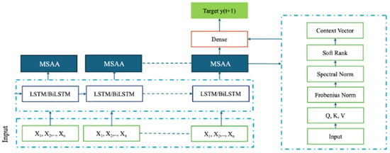
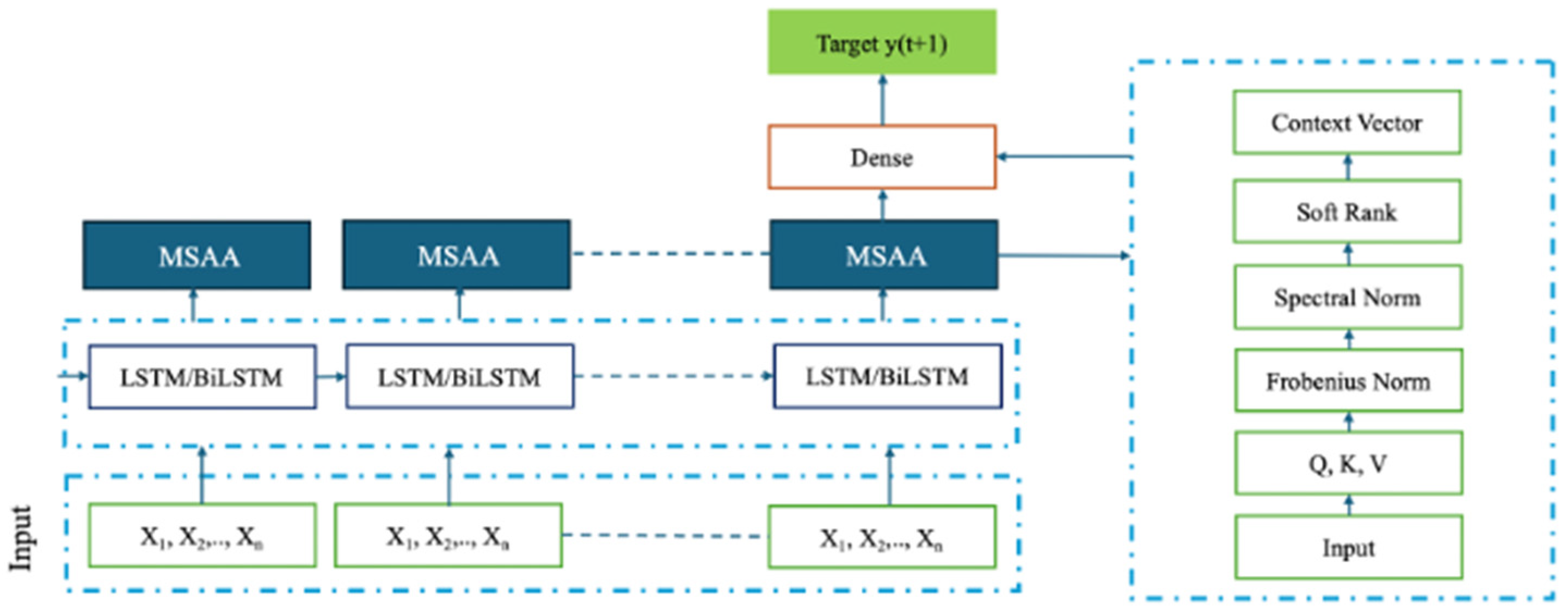
In this study, LSTM is employed as a backbone for temporal feature extraction and is further augmented with a custom attention mechanism that incorporates matrix-based statistical descriptors to enhance RUL prediction performance. In the model, each input sequence is processed by LSTM or BiLSTM layers, which capture temporal dependencies across different time windows. These layers are each followed by an MSAA module, which enriches the learned features by incorporating structural matrix statistics derived from the input matrix and integrates Query-Key-Value (QKV) attention paradigm. The schematic of the model can be seen in Figure 3.

Figure 3. Schematic representation of the MSAA with LSTM/BiLSTM model.

The selection of hyperparameters was guided by both prior literature and dataset-specific characteristics and systematically refined using a grid search strategy. The batch sizes were selected differently by grid search for C-MAPSS and N-CMAPSS to account for their distinct data scales and statistical properties. Although N-CMAPSS is substantially larger and more heterogeneous than C-MAPSS, this scale makes it more suitable for training with a larger batch size.

To clarify the core concepts and procedural flow, pseudocode is presented in Algorithms 1 and 2.

Algorithm 1. LSTM (for N-CMAPSS)/BiLSTM (for C-MAPSS)

Input: Pre-processed 3D time series data [sample, time step, feature] Orthogonal initializer for LSTM Glorot uniform initializer for Dense layers Number of epochs is 60 (for N-CMAPSS)/100 (for CMAPSS) Batch size = 256 (for N-CMAPSS)/128 (for C-MAPSS) Output: Trained LSTM model

LSTM Model: Define input layer Apply LSTM layer with 10 units (for N-CMAPSS)/64 (for C-MAPSS) Apply batch normalization Apply dropout with a ratio of 0.2 Apply a Dense layer with 50 units and ReLU activation Apply dropout with a ratio of 0.3 Output layer: Dense with 1-unit, linear activation (for regression) Compile the model using an appropriate optimizer and loss (e.g., Adam, MSE) Return the complete LSTM model

Then, a single attention layer is added to Algorithm 1 with output dimension 32 for N-CMAPSS and 16 for C-MAPSS dataset.

In Algorithm 2, matrix statistics-aware enhanced attention layer is added to existing LSTM model. In our implementation, the MSAA module is applied on top of the final LSTM (or BiLSTM) layer’s sequence output.

Algorithm 2. MSAA with LSTM (for N-CMAPSS)/BiLSTM (for C-MAPSS)

Input: Pre-processed 3D time series data [sample, time step, feature] Orthogonal initializer for LSTM Glorot uniform initializer for Dense layers Number of epochs is 60 (for N-CMAPSS)/100 (for C-MAPSS) Batch size = 256 (for N-CMAPSS)/128 (for C-MAPSS) Output: Trained matrix statistics-aware attention-enhanced LSTM model

LSTM-MSAA model: Define input layer Apply LSTM (for N-CMAPSS)/BiLSTM (for C-MAPSS) layer with 10 units (for N-CMAPSS)/64 (for C-MAPSS) Apply batch normalization Apply dropout with a ratio of 0.2 Apply MSAA layer with output dimension 32 (for N-CMAPSS)/128 (for C-MAPSS) ○ Project inputs to queries Q, keys K and values V ○ Compute scaled dot-product attention scores ○ Compute auxiliary matrix statistics ▪ Frobenius norm ▪ Spectral norm via max singular value ▪ Soft rank via normalized SVD ○ Broadcast all auxiliary statistics ○ Concatenate [S,logF,spectralN,softRank] along last axis ○ Apply LayerNormalization and a Dense layer to produce fused attention scores ○ Apply softmax to obtain attention weights ○ Compute weighted sum over values V to get attended output ○ Reduce over time axis to produce context vector Pass context vector through a Dense layer with 50 units and ReLU activation Apply dropout with a ratio of 0.3 Output layer: Dense with 1-unit, linear activation (for regression) Compile the model using an appropriate optimizer and loss (e.g., Adam, MSE) Return the complete LSTM-Attention model

Residuals are analyzed over all test windows to characterize error dynamics across the full degradation trajectory. To analyze the models’ prediction behavior in greater detail, residual distributions were examined under a fixed random seed. The random seed was selected via grid search, resulting in a value of 1024 for the C-MAPSS dataset and 34 for the N-CMAPSS dataset.

4.1. Case 1 Results

In this study, 14 onboard sensors (Table 4), which are commonly found in many commercial turbofan engines, are selected for PHM through a preprocessing method as in [54].

Table 4. Selected sensors in C-MAPSS [54].

#	Sensor Measurements	Unit
1	T24—Total temperature at LPC outlet	°R
2	T30—Total temperature at HPC outlet	°R
3	T50—Total temperature at LPT outlet	°R
4	P30—Total pressure at HPC outlet	psia
5	Nf—Physical fan speed	rpm
6	Nc—Physical core speed	rpm
7	Ps30—Static pressure at HPC outlet	psia
8	Phi—Ratio of fuel flow to Ps30	pps/psi
9	NRf—Corrected fan speed	rpm
10	NRc—Corrected core speed	rpm
11	BPR—Bypass ratio	-
12	htBleed—Burner fuel-air ratio	-
13	W31—HPT coolant bleed	lbm/s
14	W32—LPT coolant bleed	lbm/s

Sliding-window labels follow the dataset’s RUL targets. The hyperparameters used in experiments conducted with the C-MAPSS dataset are fundamental building blocks that directly affect the accuracy and overall performance of the model. Of these parameters, the window length is 30 and the window shift amount is 1, ensuring that the time series data is sampled at high resolution. The learning rate used in the model training process was initially set at 0.001 and then reduced to 0.0001 after the fifth epoch to ensure the stability of the learning process. A training period of 100 epochs was chosen, and learning was optimized for large data sets with a batch size of 128. Early RUL was determined to be 125, as in the literature [55]. Adam optimizer with an initial learning rate of 1 × 10⁻³, β₁ = 0.9, β₂ = 0.999, ε = 1 × 10⁻⁷ and a step decay to 1 × 10⁻⁴ from epoch 5 was used. All experiments are trained jointly end-to-end: the BiLSTM backbone and the MSAA module are updated simultaneously from randomly initialized weights, with MSE loss.

All other hyperparameters are shown in Table 5. All these settings are balanced to enable the model to achieve lower RMSE in the RUL task and improve its generalization ability.

Table 5. Hyperparameters of Case 1.

Hyperparameter	Value	Description
Sequence Length	30	Time-series window size for each input segment
Stride	1	Step size for sliding the time window
Batch Size	128	Number of samples per gradient update
Learning Rate	0.001	Initial learning rate for the optimizer
Optimizer	Adam (AMSGrad)	Variant of Adam with better convergence properties
Max Epochs	100	Maximum number of training epochs
Early Stopping Patience	20	Epochs to wait before stopping when no improvement on validation loss
Validation Split	0.2	Proportion of training data used for validation
Dropout Rate	0.2–0.3	Applied after BiLSTM and dense layers for regularization
BiLSTM Unit	64	Number of units in BiLSTM layer
Output Dimension	16	Output Dimension of the MSAA Layer
Dense	32	Number of units in Dense layer
Kernel Initializer (LSTM)	Orthogonal	Preserves gradient norm during training
Kernel Initializer (Dense)	Glorot Uniform	Balances signal flow for stable learning

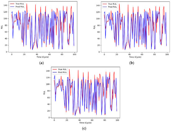
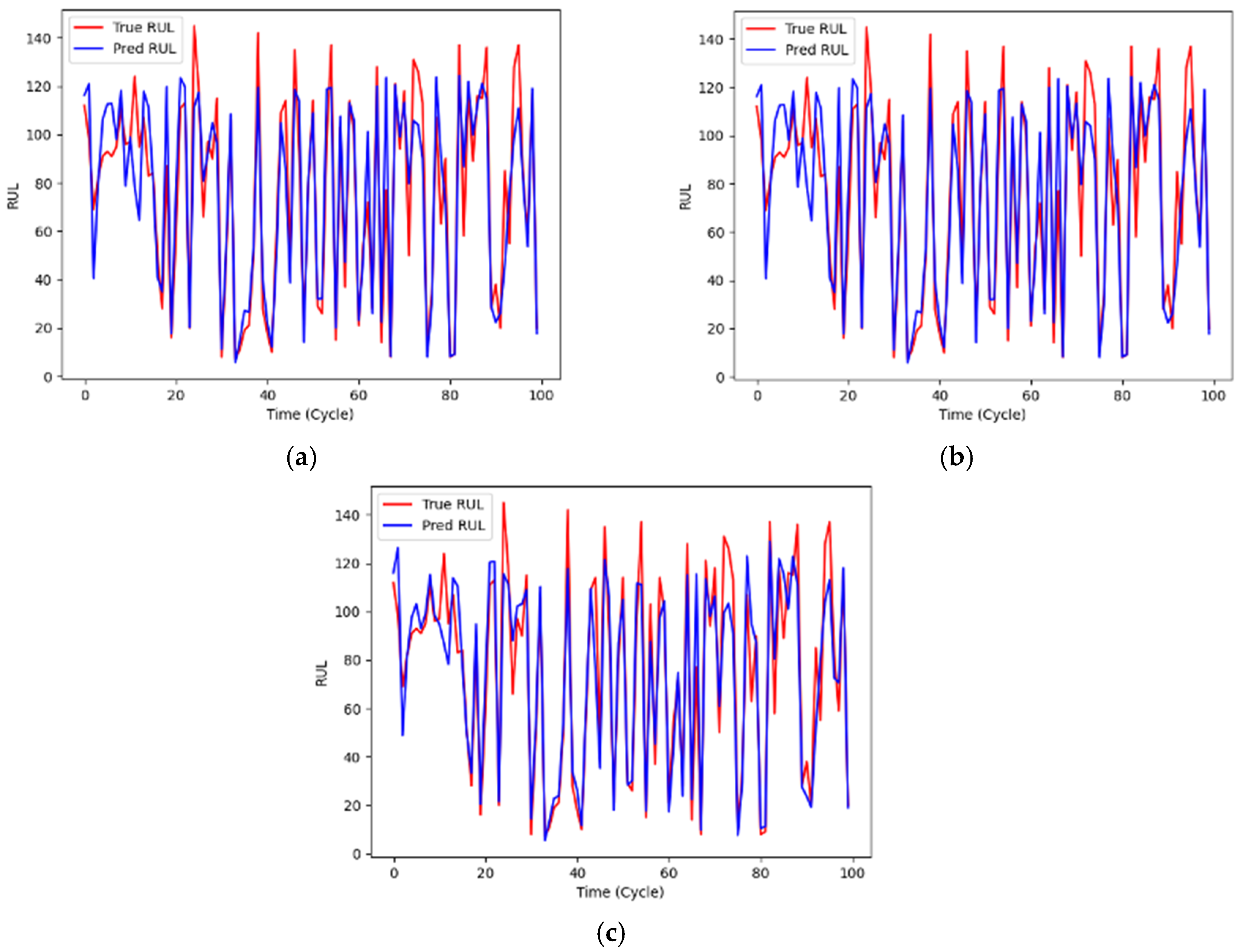
The RUL prediction plots for the LSTM, LSTM-Attention and LSTM-MSAA models can be seen in Figure 4. Degradation prediction results for representative test engines. The horizontal axis denotes the flight cycle index (time), while the vertical axis represents the predicted and true RUL in cycles.

Figure 4. RUL prediction and actual values (a) LSTM model; (b) LSTM-Attention model; (c) LSTM-MSAA model.

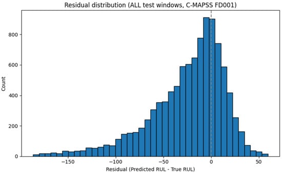
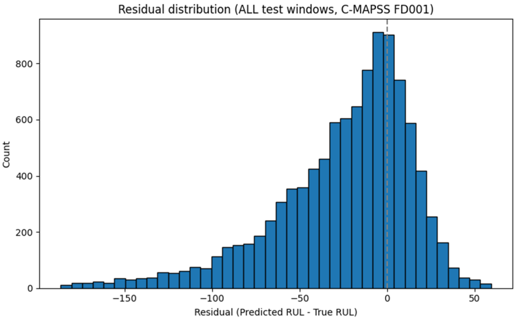
Figure 5 illustrates the residual distribution computed over all test windows of the C-MAPSS FD001 dataset.

Figure 5. Residual distributions of LSTM-MSAA model for FD001.

The distribution is noticeably left-skewed, indicating a predominantly conservative prediction behavior where the model tends to underestimate the remaining useful life. This effect is particularly pronounced at early-life stages, where degradation signatures are weak and sensor dynamics remain close to nominal operating conditions, leading to large negative residuals. In contrast, residuals concentrate around zero in the low-RUL region, demonstrating improved accuracy near end-of-life, which is the most critical phase for maintenance decision-making. Such asymmetric residual behavior is consistent with prior C-MAPSS studies and reflects the inherent difficulty of RUL estimation during early operational phases rather than model instability.

A literature comparison of studies conducted using the C-MAPSS FD001 dataset is presented in Table 6.

Table 6. Performance comparison proposed models with literature on the C-MAPSS dataset.

Proposed Method	Result (RMSE)	References
Graph Neural Networks (GNMR)	12.14	[56]
Transformer Encoder Enhanced by a Gated Convolutional Unit (GCU-Transformer)	11.27	[57]
Attention-Based LSTM	14.53	[58]
Fusing Physics-based Hybrid Model (FNN)	FNN: 17.6 ± 0.2 LSTM: 16.9 ± 0.4 CNN: 16.0 ± 0.2	[59]
Convolutional Extreme Learning Machine (MOO-CELM)	$16.54 \pm$ 0.57	[60]
Temporal and Heterogeneous Graph Neural Network (THGNN)	13.15	[61]
Federated Learning	13.38	[62]
Attention LSTM (ALSTMP)	12.11	[19]
SDPA-BiLSTM	8.98	[25]
Difference Transformer Network (Dformer)	11.02	[63]
Graph Feature Attention Network	11.71	[64]
Self-Supervised Learning	$14.34 \pm$ 0.48	[65]
Local Enhanced Channel Self-Attention Based on Transformer (LECformer)	11.31	[34]
CNN-Transformer with Wiener	11.15	[66]
Robust Uncertainity Quantification (RobustUQ)	Situation1: 12.16 Situation4: 13.68	[67]
Knowledge-Guided Dual-Path Multifeature Fusion (KDMFusion)	12.65	[68]
Operating Condition Feature Representation-Based Fourier Graph Network (OCFGNet)	10.92	[69]
GPT-Based	10.98	[70]
Dual-Dimension Convolutional-Attention-Temporal Convolutional Network (DDCA-TCN)	12.41	[71]
Deep Autoencoder (DAE)-LSTM-Quantile Regression Kernel Density Error (KDE)	13.58	[72]
Proposed Method:	LSTM: 15.338 LSTM-Attention: 15.119 LSTM-MSSA: 14.273

The RMSE results obtained in the C-MAPSS FD001 subset are presented in Table 6. According to the results of the proposed model, adding an attention layer to an LSTM model provided an improvement of approximately 1.4%. Our proposed LSTM-MSAA, on the other hand, provided an additional improvement of approximately 6.9% compared to LSTM and 5.6% compared to LSTM-Attention. Even in a cleaner scenario such as FD001′s single failure mode, MSAA’s injection of structural clues such as log-Frobenius, spectral norm, and soft rank into the attention score produced the lowest error, outperforming both the plain LSTM and the classic attention layer.

4.2. Case 2 Results

Based on the work in [59], we used six engines (u2, u5, u10, u16, u18, and u20) for the training set and three engines (u11, u14, and u15) for the test set. It should be emphasized that the evaluation outcomes provide indirect insight into the overall effectiveness of the RUL prediction models, particularly given that units u11 and u14 operate under relatively short-duration and low-altitude mission profiles, which differ from the operational conditions present in the training dataset.

The model training and evaluation pipeline was configured with hyperparameters to optimize the predictive performance on the N-CMAPSS dataset. The sequence length and stride parameters were set to 50 and 1, respectively. A batch size of 256 and an initial learning rate of 0.001 were selected. Model optimized via the AMSGrad variant of the Adam optimizer to ensure stable convergence. This was used with initial learning rate 1 × 10⁻³, β₁ = 0.9, β₂ = 0.999, ε = 1 × 10⁻⁷.

The training regime consisted of up to 60 epochs, with early stopping patience of 20 epochs based on validation loss. A learning rate decay schedule was introduced at epochs 30 and 70 to further refine optimization. A validation split of 10% was applied to monitor generalization performance. For regularization, dropout layers with rates of 0.2 to 0.3 were inserted after LSTM and dense layers, and batch normalization was used to accelerate convergence and mitigate internal covariate shift. Finally, to ensure numerical stability and prevent overfitting, orthogonal initialization was used for LSTM layers, while Glorot uniform initialization was applied to dense layers. All experiments were conducted as end-to-end joint training, where the LSTM backbone and the MSAA module are updated simultaneously from randomly initialized weights. To promote reproducibility, we fixed seeds (Python/NumPy/TensorFlow) to 0.

The configuration facilitated robust optimization and improved generalization performance in the context of RUL prediction using multivariate temporal signals. Details of the hyperparameters are presented in Table 7.

Table 7. Hyperparameters of Case 2.

Hyperparameter	Value	Description
Sequence Length	50	Time-series window size for each input segment
Stride	1	Step size for sliding the time window
Batch Size	256	Number of samples per gradient update
Learning Rate	0.001	Initial learning rate for the optimizer
Optimizer	Adam (AMSGrad)	Variant of Adam with better convergence properties
Learning Rate Decay	Epochs 30 & 70	Learning rate reduced by factor of 10 at specified epochs
Max Epochs	60	Maximum number of training epochs
Early Stopping Patience	20	Epochs to wait before stopping when no improvement on validation loss
Validation Split	0.1	Proportion of training data used for validation
Dropout Rate	0.2–0.3	Applied after LSTM and dense layers for regularization
LSTM Units	10	Number of units in LSTM layers
Output Dimension	32	Output Dimension of the MSAA Layer
Kernel Initializer (LSTM)	Orthogonal	Preserves gradient norm during training
Kernel Initializer (Dense)	Glorot Uniform	Balances signal flow for stable learning

To ensure reproducibility and isolate architectural effects from stochastic training variability, all models were trained using a fixed random seed (seed = 34). The RUL prediction results for LSTM, LSTM-Attention and LSTM-MSAA models are presented in Table 8.

Table 8. Unit-level RMSE comparison of LSTM, LSTM-Attention, and LSTM-MSAA models under fixed random seed.

Unit	LSTM (RMSE)	LSTM-Attention (RMSE)	LSTM-MSAA (RMSE)
u11	3.113	3.066	4.501
u14	12.461	9.932	5.640
u15	7.226	6.201	3.020
RMSE across all units combined	6.524	5.530	4.225

The findings in Table 8 summarize the RMSE comparison for the three units and the overall error when all units are combined. The fixed-seed evaluation highlights the contribution of each architectural component.

Overall, the lowest aggregate RMSE was achieved with LSTM-MSAA model (4.225); this corresponds to a 35.2% improvement over LSTM and a 23.6% improvement over LSTM-Attention. When looking at the unit-by-unit basis, MSAA is clearly superior in u14 and u15. In u14, algorithm reduced the values of 12.461 (LSTM) and 9.932 (LSTM-Attention) to 5.640, providing improvements of 54.7% and 43.2%, respectively. In u15, algorithm reduced the values of 7.226 (LSTM) and 6.201 (LSTM- Attention) to 3.020, achieving improvements of 58.2% and 51.3%, respectively. In u11, LSTM-Attention produced the lowest error at 3.066, while MSAA lagged at 4.501. This table shows that MSAA better captures structural clues, especially in units with pronounced heterogeneous/early late decay dynamics (u14, u15); whereas in cases with more regular patterns, such as u11, the classical attention mechanism may be sufficient. Nevertheless, when all units are evaluated together, MSAA has the highest overall generalization performance.

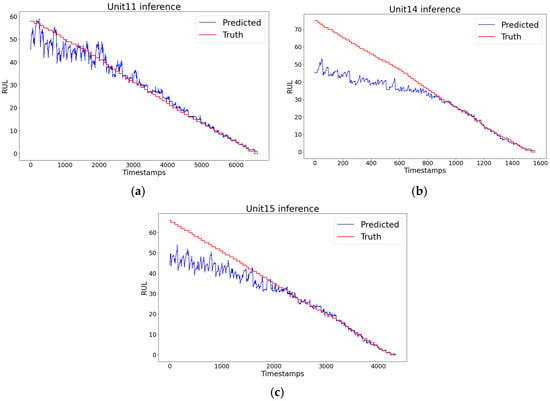
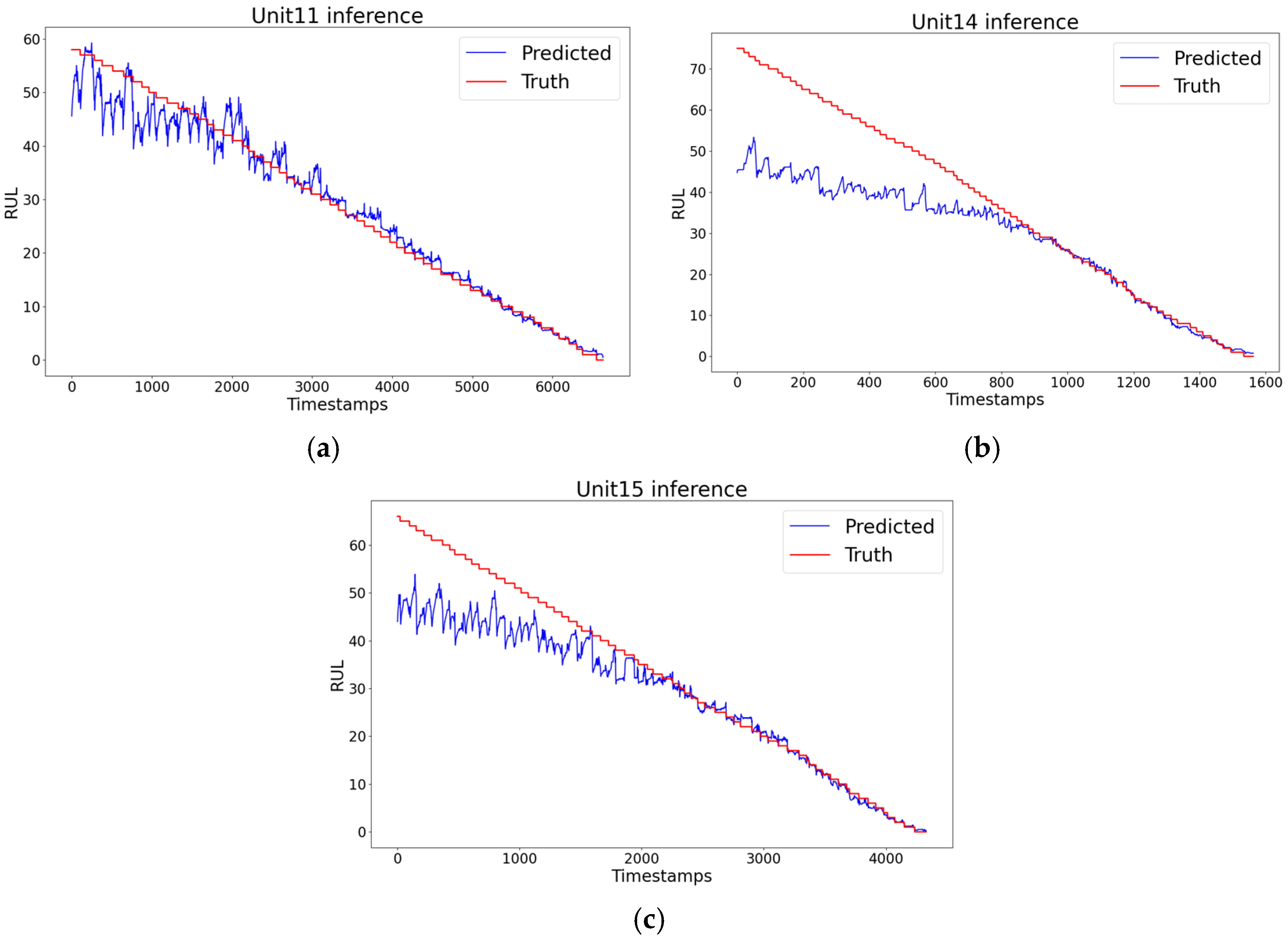
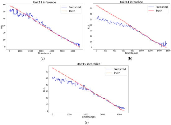
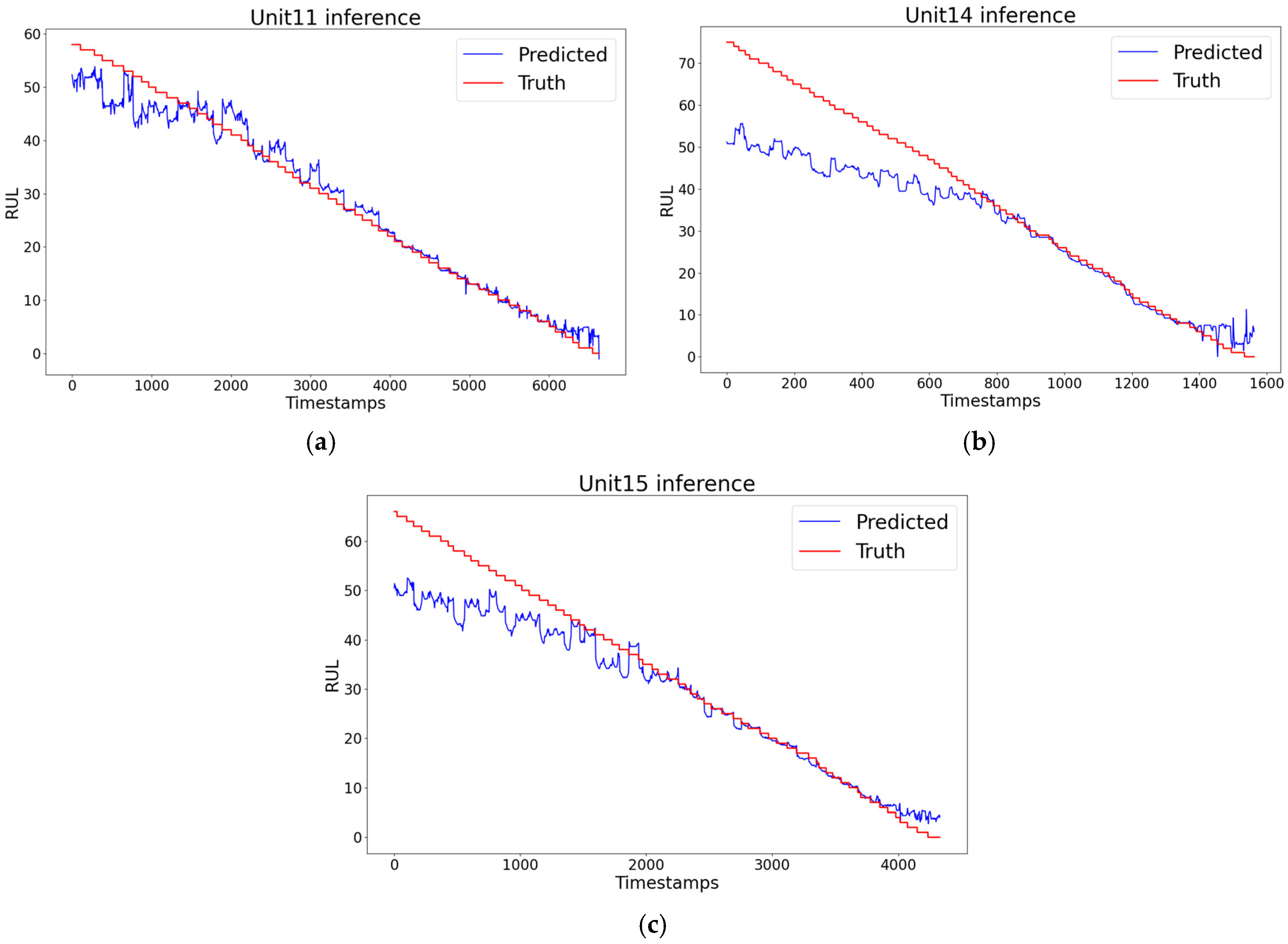
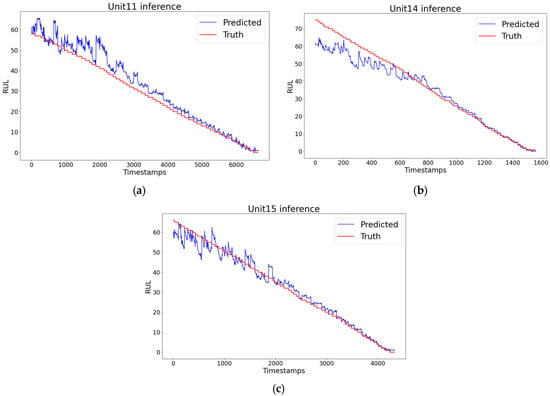
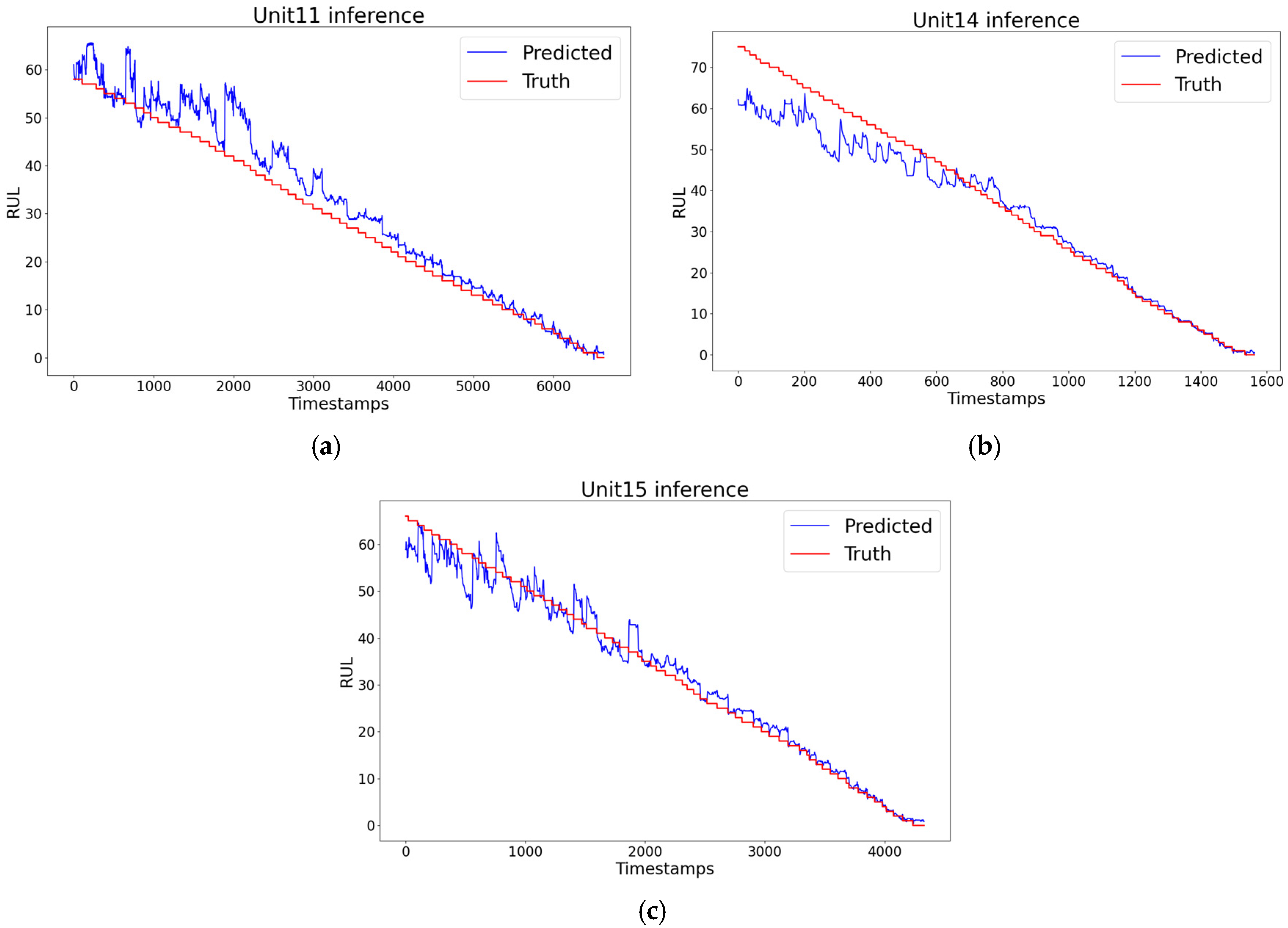
Figure 6, Figure 7 and Figure 8 present the graphical results of the training loss and RUL predictions for u11, u14 and u15. Figure 5 presents the graphical results for the LSTM model.

Figure 6. RUL prediction and actual values of the LSTM model: (a) Unit11; (b) Unit14; (c) Unit15.

Figure 7. RUL prediction and actual values of the LSTM-Attention Model: (a) Unit11; (b) Unit14; (c) Unit15.

Figure 8. RUL prediction and actual values of the LSTM-MSAA Model: (a) Unit11; (b) Unit14; (c) Unit15.

Figure 7 presents the graphical results for LSTM-Attention model and Figure 8 presents the graphical results for the LSTM-MSAA model.

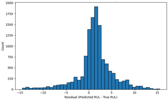
To analyze the models’ prediction behavior in greater detail, residual distributions were examined under a fixed random seed (Figure 9).

Figure 9. Residual distribution of LSTM-MSAA model for DS02.

The LSTM model exhibits a negatively skewed distribution with a residual mean of −2.82, indicating a systematic tendency to underestimate the remaining useful life. This behavior is consistent with the limited ability of standard LSTM architectures to capture complex and heterogeneous degradation patterns under varying operating conditions. Incorporating a conventional attention mechanism partially mitigates this bias, as reflected by the LSTM-Attention model’s residual mean of −2.11 and a visibly more concentrated distribution around zero. This suggests that temporal attention improves focus on informative time steps, thereby reducing but not eliminating systematic underestimation.

In contrast, the proposed LSTM-MSAA model produces a residual distribution that is more symmetric and tightly centered around zero, with a residual mean of 1.38. This near-zero biases, accompanied by a slight tendency toward overestimation, indicates improved calibration of RUL predictions. The reduced spread and increased concentration of residuals demonstrate that embedding matrix-level statistical characteristics into the attention mechanism enables the model to better capture global structural degradation information, leading to more balanced and reliable predictions across different engines and degradation regimes.

A literature comparison of studies conducted using the N-CMAPSS DS02 dataset is presented in Table 9.

Table 9. Performance comparison proposed models with literature on the N-CMAPSS dataset.

Proposed Method	Result (RMSE)	References
Deep Gaussian Process—Monte Carlo Dropout (DGPs-MCD)	7.31	[73]
Feed-Forward Neural Network (FNN) CNN	FNN: 4.22 ± 0.10 CNN: 4.14 ± 0.09	[59]
ProgNet: Transferable Deep Network	LSTM: 6.01 ProgNet: 5.64	[74]
Multi-objective optimization of extreme learning machine (MLP)	CNN: 6.29 MLP: 6.79	[75]
Spatial-Temporal Dual-Channel Adaptive Graph Convolutional Network	SDAGCN: 4.14 TCN: 7.43 GRU: 7.89	[27]
Spatial Correlation and Temporal Attention-Based LSTM (SCTA-LSTM)	LSTM: 4.81 SCA-LSTM: 4.14 CNN: 4.38 BiLSTM: 4.78	[20]
Spatio-temporal improved Transformer Model (MSTformer)	2.53	[76]
Dynamic Length Transformer-Based Network (Dlformer)	6.79	[77]
Comprehensive Dynamic Structure Graph Neural Network (CDSG)	3.96	[78]
Attention LSTM Projected Model (ALSTMP)	5.1	[19]
Multi-Resolution LSTM (MR-LSTM)	MR-LSTM: 4.52 Transformer: 5.34	[79]
THGNN	5.59	[61]
Heteroscedastic Neural Networks (HNN) Variational Bayesian Neural Networks (BNN) Monte Carlo Dropout (MCD) Deep Ensembles (DE)	DE: 8.19 ± 0.67	[80]
Local Enhanced Channel Self-Attention Based on Transformer (LECformer)	LECformer: 4.13	[34]
Operating Condition Feature Representation-Based Fourier Graph Network (OCFGNet)	2.61 ± 0.09	[69]
Knowledge-Guided Dual-Path Multifeature Fusion (KDMFusion)	5.08	[68]
Proposed Model	LSTM: 6.524 LSTM-ATTN: 5.530 LSTM-MSSA: 4.225

5. Discussion

Considering the recent focus on the growing research interest in enhancing RUL prediction models, particularly those leveraging attention-based and Transformer-inspired architectures, this study presents a comparative evaluation of recent methods published over the past five years.

Previous studies have explored spectral norms, soft-rank surrogates, and SVD-based operators within neural networks and attention mechanisms, primarily for regularization, stability control, or computational efficiency. In contrast to these approaches, the present work does not introduce a new matrix norm or rank surrogate. Instead, its novelty lies in repurposing well-established matrix-level descriptors as degradation-aware contextual signals within the attention computation for turbofan RUL prediction.

In the proposed MSAA framework, Frobenius norm, spectral norm and soft rank descriptors are computed directly from each multivariate sensor window and treated as global, input-dependent scalar features. They are fused with the attention score tensor through a lightweight fusion network, enabling the model to capture global energy, dominant variance direction, and effective dimensionality of each time window. This design allows the attention mechanism to remain compact and fully compatible with LSTM and BiLSTM backbones, without requiring explicit graph construction or handcrafted feature extraction. To the best of our knowledge, such as matrix-statistics-aware attention formulation has not been previously reported for C-MAPSS or N-CMAPSS RUL prediction tasks, where attention is typically defined purely via pairwise temporal or spatial similarities.

From a computational perspective, the baseline LSTM model exhibits a very low computational footprint reflecting its limited representational capacity. Incorporating a conventional attention mechanism increases the computational cost due to the explicit modeling of pairwise temporal dependencies. The proposed LSTM-MSAA further increases the FLOPs as additional matrix-level statistical operations.

Table 6 presents a comparative analysis of RMSE values reported by recent methods on the C-MAPSS dataset, published between 2020 and 2025.

Compared with the baseline LSTM model, the proposed LSTM-MSAA achieves a clear and consistent improvement, reducing RMSE from 15.338 (LSTM) to 14.273. This result also outperforms conventional attention-based LSTM variants [58], indicating that incorporating matrix-level statistical descriptors into the attention mechanism provides additional discriminative power beyond similarity-driven attention alone. While several state-of-the-art approaches, such as SDPA-BiLSTM [25], OCFGNet [69], and Dformer [63], report lower RMSE values, these methods typically rely on substantially more complex architectures, including multi-stage attention pipelines, graph construction, frequency-domain transformations, or extensive feature engineering. However, the ALSTMP model reported in [19] achieves lower RMSE values than the proposed approach, which can be partially attributed to its use of a longer sliding window length, allowing the model to capture a broader temporal context compared to the configuration adopted in this study. Transformer-based solutions further improved the generalization ability, as seen in GCUTransformer [57], LECformer [34], CNN-Transformer with Wiener [66] and Dformer [63], both emphasizing convolutional and temporal dynamics. More recent methods such as OCFGNet [69] and GPT-Based [70] method reached other best results.

Table 9 presents a comparative evaluation of recent RUL prediction models on the N-CMAPSS dataset. N-CMAPSS Unit11, which belongs to flight class 3 representing a long mission profile, Unit14, associated with a short-duration profile (flight class 1), begins to degrade later. Unit 15, categorized as a medium-length profile (flight class 2). These differences imply that the point at which degradation initiates is influenced by the type of operational profile, with shorter missions such as that of Unit14 and tending to preserve engine health for longer durations. The divergence between the degradation behaviors of Unit11 and Unit14 contributes to inconsistency in model predictions across units, which in turn negatively impacts overall performance. For this reason, some studies excluded Unit14 from their experimental studies [28,63]. Among the reported approaches, MSTFormer achieves the lowest RMSE, reflecting its strong capability to model complex spatio-temporal dependencies through a multi-branch Transformer architecture [76]. Similarly, graph-based models such as SDAGCN [27], OCFGNet [69], and CDSG [78] demonstrate superior predictive accuracy by explicitly modeling inter-sensor relationships and operating-condition-dependent structures. The transformer-based LECformer solution further improved the generalization ability as in the C-MAPSS experiments [34]. It is also noteworthy that many of the high-performing models rely on sophisticated architectures involving graph construction, Fourier-domain representations, or deep Transformer stacks, which substantially increase model complexity and computational cost. In contrast, the proposed MSAA-based model achieves competitive performance with 4.225 RMSE using a comparatively lightweight LSTM-based architecture, without requiring explicit graph modeling or multi-resolution feature fusion. The results of this study indicate that attention mechanisms can be enhanced not only through architectural complexity, but also by embedding mathematically grounded matrix-level descriptors directly into the attention computation.

In realistic industrial environments, RUL prediction models are often exposed to continuously evolving operating conditions, sensor drift, and progressive changes in degradation patterns. Recent studies have highlighted that static, offline-trained models may suffer from performance degradation when deployed over long operational horizons. To address this issue, continual learning frameworks have been proposed to enable incremental adaptation while mitigating catastrophic forgetting [81]. Given that the proposed MSAA mechanism explicitly captures structural changes in multivariate sensor representations, integrating continual learning strategies constitutes a promising future direction to enhance long-term robustness under non-stationary conditions.

6. Conclusions

The widespread usage of sensors with intelligent algorithms in the systems helps to predict the future condition of the components with data-driven approaches. PHM extends the life of the system components by reducing the maintenance costs, increasing system safety and extending the time between maintenance intervals with the reliable prediction of the RUL.

In this study, we proposed an original MSAA mechanism integrated with LSTM and BiLSTM architectures to enhance RUL prediction performance in turbofan engines. The primary contribution of this work is the integration of matrix-level statistical descriptors, which are Frobenius norm, spectral norm, and soft rank, into the computation of attention scores. This approach enables the model to not only learn temporal dependencies but also capture the structural properties embedded in the sensor data, thereby contributing to improved interpretability and predictive robustness. The proposed model was evaluated on two benchmark datasets, C-MAPSS and N-CMAPSS, both of which are widely used in the PHM literature. The experimental results demonstrated that the proposed architecture outperforms baseline LSTM and conventional attention-enhanced LSTM model in terms of RMSE.

Future work will focus on improving the scalability of the proposed MSAA mechanism by integrating it with efficient Transformer-based attention variants, while preserving its ability to capture matrix-level structural characteristics. In addition, incorporating continual learning strategies will enable the model to adapt to evolving operating conditions and sensor drift without retraining from scratch, thereby enhancing long-term robustness for real-world PHM applications.

References

- Bridgman, M.S. Relating failure prognostics to system benefits. In Proceedings of the Aerospace Conference, Big Sky, MT, USA, 9–16 March 2002; IEEE: New York, NY, USA, 2002; p. 7. [Google Scholar] [CrossRef] [Scilit]
- Zio, E. Prognostics and health management (PHM): Where are we and where do we (need to) go in theory and practice. Reliab. Eng. Syst. Saf. 2022, 218, 108119. [Google Scholar] [CrossRef] [Scilit]
- Lee, J.; Wu, F.; Zhao, W.; Ghaffari, M.; Liao, L.; Siegel, D. Prognostics and health management design for rotary machinery systems—Reviews, methodology and applications. Mech. Syst. Signal Process. 2014, 42, 314–334. [Google Scholar] [CrossRef] [Scilit]
- Nguyen, V.D.; Kefalas, M.; Yang, K.; Apostolidis, A.; Olhofer, M.; Limmer, S.; Bäck, T. A review: Prognostics and health management in automotive and aerospace. Int. J. Progn. Health Manag. 2019, 10, 35. [Google Scholar] [CrossRef] [Scilit]
- Fu, S.; Avdelidis, N.P. Prognostic and health management of critical aircraft systems and components: An overview. Sensors 2023, 23, 8124. [Google Scholar] [CrossRef] [Scilit]
- Sutharssan, T.; Stoyanov, S.; Bailey, C.; Yin, C. Prognostic and health management for engineering systems: A review of the data-driven approach and algorithms. J. Eng. 2015, 2015, 215–222. [Google Scholar] [CrossRef] [Scilit]
- Javed, K.; Gouriveau, R.; Zerhouni, N. State of the art and taxonomy of prognostics approaches, trends of prognostics applications and open issues towards maturity at different technology readiness levels. Mech. Syst. Signal Process. 2017, 94, 214–236. [Google Scholar] [CrossRef] [Scilit]
- Ferreira, C.; Gonçalves, G. Remaining Useful Life prediction and challenges: A literature review on the use of Machine Learning Methods. J. Manuf. Syst. 2022, 63, 550–562. [Google Scholar] [CrossRef] [Scilit]
- Malhotra, P.; Vig, L.; Shroff, G.; Agarwal, P. Long short term memory networks for anomaly detection in time series. In Proceedings of the European Symposium on Artificial Neural Networks, Computational Intelligence and Machine Learning (ESANN), Bruges, Belgium, 26–28 April 2017. [Google Scholar]
- Zhang, L.; Lin, J.; Liu, B.; Zhang, Z.; Yan, X.; Wei, M. A review on deep learning applications in prognostics and health management. IEEE Access 2019, 7, 162415–162438. [Google Scholar] [CrossRef] [Scilit]
- Wang, X.; Li, Y.; Xu, Y.; Liu, X.; Zheng, T.; Zheng, B. Remaining useful life prediction for aero-engines using a time-enhanced multi-head self-attention model. Aerospace 2023, 10, 80. [Google Scholar] [CrossRef] [Scilit]
- Wang, Y.; Zhao, Y.; Addepalli, S. Remaining useful life prediction using deep learning approaches: A review. Procedia Manuf. 2020, 49, 81–88. [Google Scholar] [CrossRef] [Scilit]
- Vaswani, A.; Shazeer, N.; Parmar, N.; Uszkoreit, J.; Jones, L.; Gomez, A.N.; Kaiser, Ł.; Polosukhin, I. Attention is All You Need. arXiv 2017, arXiv:1706.03762. [Google Scholar] [CrossRef] [Scilit]
- Bao, P.; Yi, W.; Zhu, Y.; Shen, Y.; Chai, B.X. STHFD: Spatial–Temporal Hypergraph-Based Model for Aero-Engine Bearing Fault Diagnosis. Aerospace 2025, 12, 612. [Google Scholar] [CrossRef] [Scilit]
- NASA. PCOE Data Set Repository. NASA Intelligent Systems Division. Available online: https://www.nasa.gov/intelligent-systems-division/discovery-and-systems-health/pcoe/pcoe-data-set-repository/ (accessed on 17 February 2025).
- Frederick, D.K.; DeCastro, J.A.; Litt, J.S. User’s Guide for the Commercial Modular Aero-Propulsion System Simulation (C-MAPSS); NASA Technical Report: Washington, DC, USA, 2007. [Google Scholar]
- Fan, Z.; Li, W.; Chang, K.-C. A two-stage attention-based hierarchical transformer for turbofan engine remaining useful life prediction. Sensors 2024, 24, 824. [Google Scholar] [CrossRef] [Scilit]
- Zhang, C.; Guo, Y.; Zhang, Y. Lab-ver: An LSTM attention based on variational autoencoder representation learning of remaining useful life estimation. Eng. Res. Express 2025, 7, 015577. [Google Scholar] [CrossRef] [Scilit]
- Tseng, S.H.; Tran, K.D. Predicting maintenance through an attention long short-term memory projected model. J. Intell. Manuf. 2024, 35, 807–824. [Google Scholar] [CrossRef] [Scilit]
- Tian, H.; Yang, L.; Ju, B. Spatial correlation and temporal attention-based LSTM for remaining useful life prediction of turbofan engine. Measurement 2023, 214, 112816. [Google Scholar] [CrossRef] [Scilit]
- Peringal, A.; Mohiuddin, M.B.; Hassan, A. Remaining useful life prediction for aircraft engines using LSTM. arXiv 2024, arXiv:2401.07590. [Google Scholar] [CrossRef] [Scilit]
- Wahid, A.; Yahya, M.; Breslin, J.G.; Ali, M.I. Self-attention transformer-based architecture for remaining useful life estimation of complex machines. Procedia Comput. Sci. 2022, 217, 456–464. [Google Scholar] [CrossRef] [Scilit]
- Zhang, Y.; Wang, X.; Liu, Y.; Li, H. Remaining useful life prediction of aircraft engine based on Bi-LSTM network integrated with attention mechanism. In Proceedings of the ASME Turbo Expo 2024: Turbomachinery Technical Conference and Exposition, London, UK, 24–28 June 2024. [Google Scholar] [CrossRef] [Scilit]
- Fan, Y.; Tang, Q.; Guo, Y.; Wei, Y. BiLSTM-MLAM: A multi-scale time series prediction model for sensor data based on Bi-LSTM and local attention mechanisms. Sensors 2024, 24, 3962. [Google Scholar] [CrossRef] [Scilit] [PubMed]
- Yang, W.; Zhou, Q.; Chen, G.; Liu, C.; Qu, C. SDPA-BiLSTM: Improving accuracy of aircraft engine remaining life prediction with enhanced attention mechanism. In Proceedings of the 9th International Conference on Computer and Communication Systems (ICCCS), Xi’an, China, 19–22 April 2024; pp. 569–574. [Google Scholar] [CrossRef] [Scilit]
- Ji, S.; Han, X.; Hou, Y.; Song, Y.; Du, Q. Remaining useful life prediction of airplane engine based on PCA–BLSTM. Sensors 2020, 20, 4537. [Google Scholar] [CrossRef] [Scilit]
- Zhang, X.; Leng, Z.; Zhao, Z.; Li, M.; Yu, D.; Chen, X. Spatial-temporal dual-channel adaptive graph convolutional network for remaining useful life prediction with multi-sensor information fusion. Adv. Eng. Inform. 2023, 57, 102120. [Google Scholar] [CrossRef] [Scilit]
- Zhou, Z.; Li, T.; Zhao, Z.; Sun, C.; Chen, X.; Yan, R.; Jia, J. Time-varying trajectory modeling via dynamic governing network for remaining useful life prediction. Mech. Syst. Signal Process. 2023, 182, 109610. [Google Scholar] [CrossRef] [Scilit]
- Shaw, P.; Uszkoreit, J.; Vaswani, A. Self-attention with Relative Position Representations. arXiv 2018, arXiv:1803.02155. [Google Scholar] [CrossRef] [Scilit]
- Wang, S.; Li, B.Z.; Khabsa, M.; Fang, H.; Ma, H. Linformer: Self-Attention with Linear Complexity. arXiv 2020, arXiv:2006.04768. [Google Scholar] [CrossRef] [Scilit]
- Fu, K.; Li, H.; Bai, Y. Mixformer: An improved self-attention architecture applied to multivariate chaotic time series prediction. Expert Syst. Appl. 2024, 241, 122484. [Google Scholar] [CrossRef] [Scilit]
- Chen, Y.; Tao, Q.; Tonin, F.; Suykens, J. Primal-attention: Self-attention through asymmetric kernel SVD in primal representation. Adv. Neural Inf. Process. Syst. 2023, 36, 65088–65101. [Google Scholar]
- Aranda, J. Singular value decomposition (SVD) as a key to efficient attention mechanisms and hierarchical structure learning. ResearchGate 2024. [Google Scholar] [CrossRef]
- Zhang, Z.; Song, W.; Wu, Q.; Sun, W.; Li, Q.; Jia, L. A novel local enhanced channel self-attention based on Transformer for industrial remaining useful life prediction. Eng. Appl. Artif. Intell. 2025, 141, 109815. [Google Scholar] [CrossRef] [Scilit]
- Cheng, X.; Chaw, J.K.; Sahrani, S.; Ang, M.C.; Gunasekaran, S.S.; Mahmoud, M.A.; Zaman, H.B.; Zhao, Y.; Ren, F. An adaptive dual distillation framework for efficient remaining useful life prediction. Complex Intell. Syst. 2025, 11, 253. [Google Scholar] [CrossRef] [Scilit]
- Kim, E.; Park, S.; Lee, H.; Ko, S.; Hwang, E. Enhanced Remaining Useful Life Prediction for Turbofan Engines Using Spatio-Temporal Koopman Dual-branch Transformer. IEEE Trans. Instrum. Meas. 2025, 74, 2550316. [Google Scholar] [CrossRef] [Scilit]
- Blondel, M.; Teboul, O.; Berthet, Q.; Djolonga, J. Fast differentiable sorting and ranking. In Proceedings of the 37th International Conference on Machine Learning, Vienna, Austria, 12–18 July 2020; PMLR: Cambridge, MA, USA, 2020; pp. 950–959. [Google Scholar]
- Tefera, Y.; Van Baelen, Q.; Meire, M.; Luca, S.; Karsmakers, P. Constraint-guided learning of data-driven health indicator models: An application on bearings. Int. J. Progn. Health Manag. 2025, 16, 1–20. [Google Scholar] [CrossRef] [Scilit]
- Arias Chao, M.; Kulkarni, C.; Goebel, K.; Fink, O. Aircraft engine run-to-failure dataset under real flight conditions for prognostics and diagnostics. Data 2021, 6, 5. [Google Scholar] [CrossRef] [Scilit]
- Vollert, S.; Theissler, A. Challenges of machine learning-based RUL prognosis: A review on NASA’s C-MAPSS data set. In Proceedings of the 2021 26th IEEE International Conference on Emerging Technologies and Factory Automation (ETFA), Vasteras, Sweden, 7–10 September 2021; IEEE: New York, NY, USA, 2021; pp. 1–8. [Google Scholar]
- Saxena, A.; Goebel, K.; Simon, D.; Eklund, N. Damage propagation modeling for aircraft engine run-to-failure simulation. In Proceedings of the International Conference on Prognostics and Health Management, Denver, CO, USA, 6–9 October 2008; pp. 1–9. [Google Scholar]
- Zhang, A.; Wang, H.; Li, S.; Cui, Y.; Liu, Z.; Yang, G.; Hu, J. Transfer learning with deep recurrent neural networks for remaining useful life estimation. Appl. Sci. 2018, 8, 2416. [Google Scholar] [CrossRef] [Scilit]
- Ramasso, E.; Saxena, A. Performance benchmarking and analysis of prognostic methods for C-MAPSS datasets. Int. J. Progn. Health Manag. 2014, 5, 1–15. [Google Scholar] [CrossRef] [Scilit]
- Hochreiter, S.; Schmidhuber, J. Long short-term memory. Neural Comput. 1997, 9, 1735–1780. [Google Scholar] [CrossRef] [Scilit]
- Goodfellow, I.; Bengio, Y.; Courville, A. Deep Learning; MIT Press: Cambridge, MA, USA, 2016; Chapter 10. [Google Scholar]
- Hatipoğlu, A.; Süpürtülü, M.; Yılmaz, E. Enhanced fault classification in bearings: A multi-domain feature extraction approach with LSTM-attention and LASSO. Arab. J. Sci. Eng. 2024, 50, 10795–10812. [Google Scholar] [CrossRef] [Scilit]
- Dai, Z.; Yang, Z.; Yang, Y.; Carbonell, J.; Le, Q.V.; Salakhutdinov, R. Transformer-XL: Attentive language models beyond a fixed-length context. arXiv 2019, arXiv:1901.02860. [Google Scholar] [CrossRef] [Scilit]
- Ding, Z.; Yu, Y.; Xia, Y. Nonlinear hysteretic parameter identification using an attention-based long short-term memory network and principal component analysis. Nonlinear Dyn. 2023, 111, 4559–4576. [Google Scholar] [CrossRef] [Scilit]
- Thoiyab, N.M.; Shanmugam, S.; Vadivel, R.; Gunasekaran, N. Frobenius norm-based global stability analysis of delayed bidirectional associative memory neural networks. Symmetry 2025, 17, 183. [Google Scholar] [CrossRef] [Scilit]
- Ford, W. Numerical Linear Algebra with Applications: Using MATLAB and Octave; Academic Press: Cambridge, MA, USA, 2014; p. 127. [Google Scholar]
- Fang, J.; Zeng, D.; Yan, X.; Zhang, Y.; Liu, H.; Tang, B.; Yang, M.; Liu, J. Combating spatial redundancy with spectral norm attention in convolutional learners. Neurocomputing 2022, 511, 105–116. [Google Scholar] [CrossRef] [Scilit]
- Golub, G.H.; Van Loan, C.F. Matrix Computations, 4th ed.; Johns Hopkins University Press: Baltimore, MD, USA, 2013. [Google Scholar]
- Mohr, D.L.; Wilson, W.J.; Freund, R.J. Statistical Methods, 4th ed.; Academic Press: Cambridge, MA, USA, 2021. [Google Scholar]
- Huang, Y.; Tao, J.; Sun, G.; Zhang, H.; Hu, Y. A prognostic and health management framework for aero-engines based on a dynamic probability model and LSTM network. Aerospace 2022, 9, 316. [Google Scholar] [CrossRef] [Scilit]
- Zhou, L.; Wang, H.; Xu, S. Aero-engine prognosis strategy based on multi-scale feature fusion and multi-task parallel learning. Reliab. Eng. Syst. Saf. 2023, 234, 109182. [Google Scholar] [CrossRef] [Scilit]
- Narwariya, J.; Malhotra, P.; TV, V.; Vig, L.; Shroff, G. Graph neural networks for leveraging industrial equipment structure: An application to remaining useful life estimation. arXiv 2020, arXiv:2006.16556. [Google Scholar] [CrossRef] [Scilit]
- Mo, Y.; Wu, Q.; Li, X.; Huang, B. Remaining useful life estimation via transformer encoder enhanced by a gated convolutional unit. J. Intell. Manuf. 2021, 32, 1997–2006. [Google Scholar] [CrossRef] [Scilit]
- Chen, Z.; Wu, M.; Zhao, R.; Guretno, F.; Yan, R.; Li, X. Machine remaining useful life prediction via an attention-based deep learning approach. IEEE Trans. Ind. Electron. 2021, 68, 2521–2531. [Google Scholar] [CrossRef] [Scilit]
- Chao, M.A.; Kulkarni, C.; Goebel, K.; Fink, O. Fusing physics-based and deep learning models for prognostics. Reliab. Eng. Syst. Saf. 2022, 217, 107961. [Google Scholar] [CrossRef] [Scilit]
- Mo, H.; Iacca, G. Evolutionary optimization of convolutional extreme learning machine for remaining useful life prediction. SN Comput. Sci. 2023, 5, 54. [Google Scholar] [CrossRef] [Scilit]
- Wen, Z.; Fang, Y.; Wei, P.; Liu, F.; Chen, Z.; Wu, M. Temporal and heterogeneous graph neural network for remaining useful life prediction. arXiv 2024, arXiv:2405.04336. [Google Scholar] [CrossRef] [Scilit]
- Söderkvist Vermelin, W.; Mishra, M.; Eng, M.P.; Andersson, D.; Kyprianidis, K. Collaborative training of data-driven remaining useful life prediction models using federated learning. Int. J. Progn. Health Manag. 2024, 15, 1–20. [Google Scholar] [CrossRef] [Scilit]
- Liu, H.; Sun, Y.; Ding, W.; Wu, H.; Zhang, H. Enhancing non-stationary feature learning for remaining useful life prediction of aero-engine under multiple operating conditions. Measurement 2024, 227, 114242. [Google Scholar] [CrossRef] [Scilit]
- Wang, Y.; Peng, S.; Wang, H.; Zhang, M.; Cao, H.; Ma, L. Remaining useful life prediction based on graph feature attention networks with missing multi-sensor features. Reliab. Eng. Syst. Saf. 2025, 258, 110902. [Google Scholar] [CrossRef] [Scilit]
- Liu, C.L.; Xiao, B.; Hsu, S.S. Self-supervised learning for remaining useful life prediction using simple triplet networks. Adv. Eng. Inform. 2025, 64, 103038. [Google Scholar] [CrossRef] [Scilit]
- Yang, X.; Gao, X.; Zheng, H.; Yang, M.; Liu, Y. A hybrid prognosis method based on health indicator and Wiener process: The case of multi-sensor monitored aero-engine. Eng. Appl. Artif. Intell. 2025, 144, 110099. [Google Scholar] [CrossRef] [Scilit]
- Wang, W.; Wang, Z.; Cai, Z.; Hu, C.; Si, S. Robust uncertainty quantification for online remaining useful life prediction with randomly missing and partially faulty sensor data. Reliab. Eng. Syst. Saf. 2025, 262, 111177. [Google Scholar] [CrossRef] [Scilit]
- Zhou, W.; Zhou, L.; Li, B.; Chen, Z.; Li, H.; Cui, W. KDMFusion: Knowledge-guided dual-path multi-feature fusion framework for remaining useful life prediction. IEEE Sensors J. 2025, 25, 16321–16334. [Google Scholar] [CrossRef] [Scilit]
- Liu, H.; Sun, Y.; Wang, X.; Wu, H.; Guo, Y.; Wang, H. Operating condition feature representation-based Fourier graph network for civil aircraft state estimation. Reliab. Eng. Syst. Saf. 2025, 261, 111085. [Google Scholar] [CrossRef] [Scilit]
- Cui, H.; Guo, X.; Yu, L. Leveraging Pre-Trained GPT Models for Equipment Remaining Useful Life Prognostics. Electronics 2025, 14, 1265. [Google Scholar] [CrossRef] [Scilit]
- Zhu, Y.; Liu, Z. A dual-dimension convolutional-attention module for remaining useful life prediction of aeroengines. Aerospace 2024, 11, 809. [Google Scholar] [CrossRef] [Scilit]
- Chen, C.; Shi, J.; Shen, M.; Feng, L.; Tao, G. A predictive maintenance strategy using deep learning quantile regression and kernel density estimation for failure prediction. IEEE Trans. Instrum. Meas. 2023, 72, 3506512. [Google Scholar] [CrossRef] [Scilit]
- Biggio, L.; Wieland, A.; Chao, M.A.; Kastanis, I.; Fink, O. Uncertainty-aware prognosis via deep Gaussian process. IEEE Access 2021, 9, 123517–123527. [Google Scholar] [CrossRef] [Scilit]
- Berghout, T.; Mouss, M.D.; Mouss, L.H.; Benbouzid, M. ProgNet: A transferable deep network for aircraft engine damage propagation prognosis under real flight conditions. Aerospace 2022, 10, 10. [Google Scholar] [CrossRef] [Scilit]
- Mo, H.; Iacca, G. Multi-objective optimization of extreme learning machine for remaining useful life prediction. In Proceedings of the International Conference on Applications of Evolutionary Computation (Part of EvoStar), Madrid, Spain, 20–22 April 2022; Springer: Cham, Switzerland, 2022; pp. 191–206. [Google Scholar]
- Xu, D.; Xiao, X.; Liu, J.; Sui, S. Spatio-temporal degradation modeling and remaining useful life prediction under multiple operating conditions based on attention mechanism and deep learning. Reliab. Eng. Syst. Saf. 2023, 229, 108886. [Google Scholar] [CrossRef] [Scilit]
- Ren, L.; Wang, H.; Huang, G. DLformer: A dynamic length transformer-based network for efficient feature representation in remaining useful life prediction. IEEE Trans. Neural Networks Learn. Syst. 2023, 35, 5942–5952. [Google Scholar] [CrossRef] [Scilit]
- Wang, H.; Zhang, Z.; Li, X.; Deng, X.; Jiang, W. Comprehensive dynamic structure graph neural network for aero-engine remaining useful life prediction. IEEE Trans. Instrum. Meas. 2023, 72, 3533816. [Google Scholar] [CrossRef] [Scilit]
- Xu, T.; Han, G.; Zhu, H.; Taleb, T.; Peng, J. Multi-resolution LSTM-based prediction model for remaining useful life of aero-engine. IEEE Trans. Veh. Technol. 2024, 73, 1931–1941. [Google Scholar] [CrossRef] [Scilit]
- Basora, L.; Viens, A.; Chao, M.A.; Olive, X. A benchmark on uncertainty quantification for deep learning prognostics. Reliab. Eng. Syst. Saf. 2025, 253, 110513. [Google Scholar] [CrossRef] [Scilit]
- Ren, X.; Qin, Y.; Li, B.; Wang, B.; Yi, X.; Jia, L. A core space gradient projection-based continual learning framework for remaining useful life prediction of machinery under variable operating conditions. Reliab. Eng. Syst. Saf. 2024, 252, 110428. [Google Scholar] [CrossRef] [Scilit]
Disclaimer/Publisher’s Note: The statements, opinions and data contained in all publications are solely those of the individual author(s) and contributor(s) and not of MDPI and/or the editor(s). MDPI and/or the editor(s) disclaim responsibility for any injury to people or property resulting from any ideas, methods, instructions or products referred to in the content. |
© 2025 by the authors. Licensee MDPI, Basel, Switzerland. This article is an open access article distributed under the terms and conditions of the Creative Commons Attribution (CC BY) license.