


Design and Simulation Verification of Model Predictive Attitude Control Based on Feedback Linearization for Quadrotor UAV

Abstract
1. Introduction
2. Dynamics Model of Quadrotor UAV
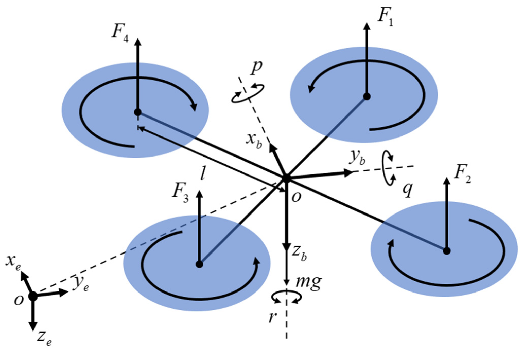
2.1. Modeling of Attitude Motion Characteristics
2.2. Model Linear Transformation
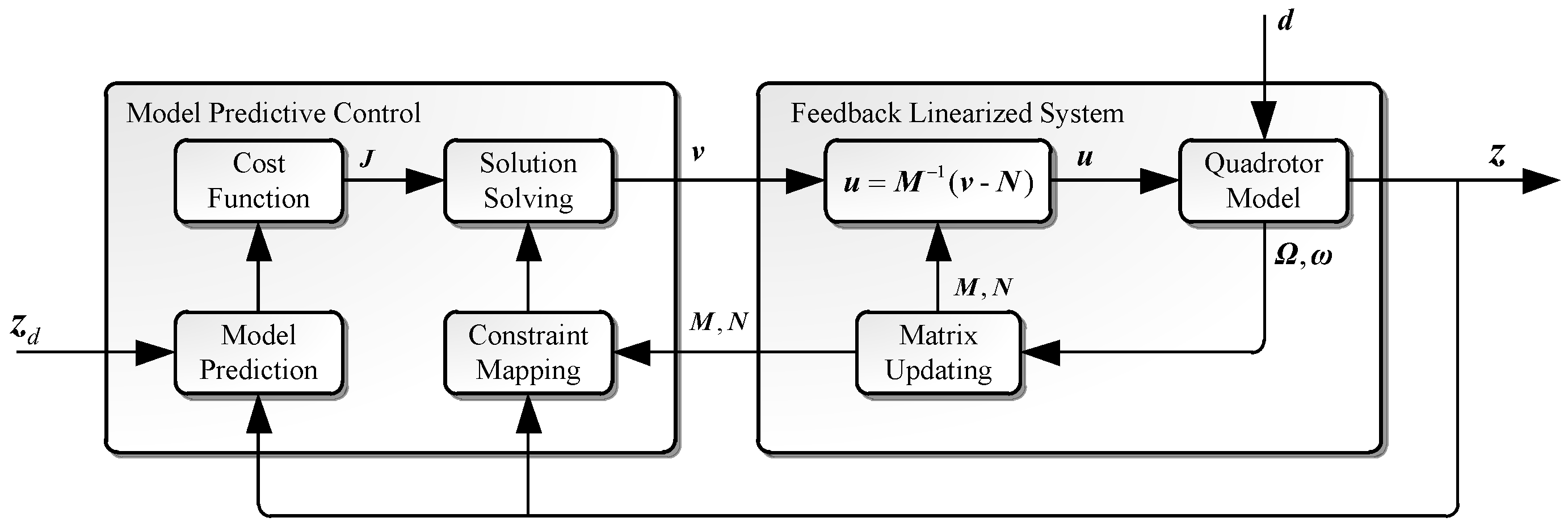
3. Attitude Controller Design
3.1. Prediction Equation for the Feedback Linearized Model
3.2. Model Predictive Control Performance
3.3. Constrained Virtual Control Solution
4. Simulation and Results Analysis
4.1. Methods
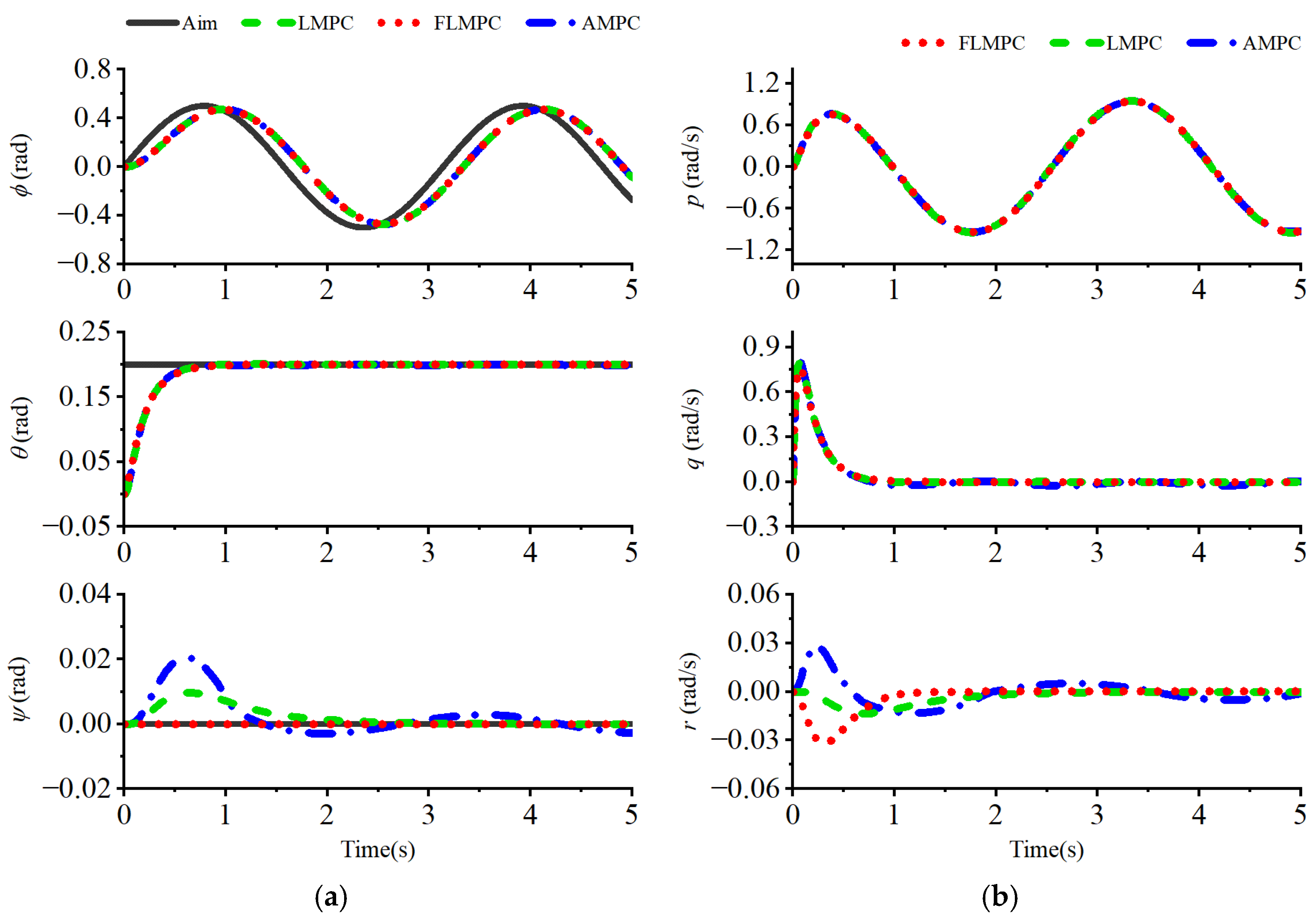
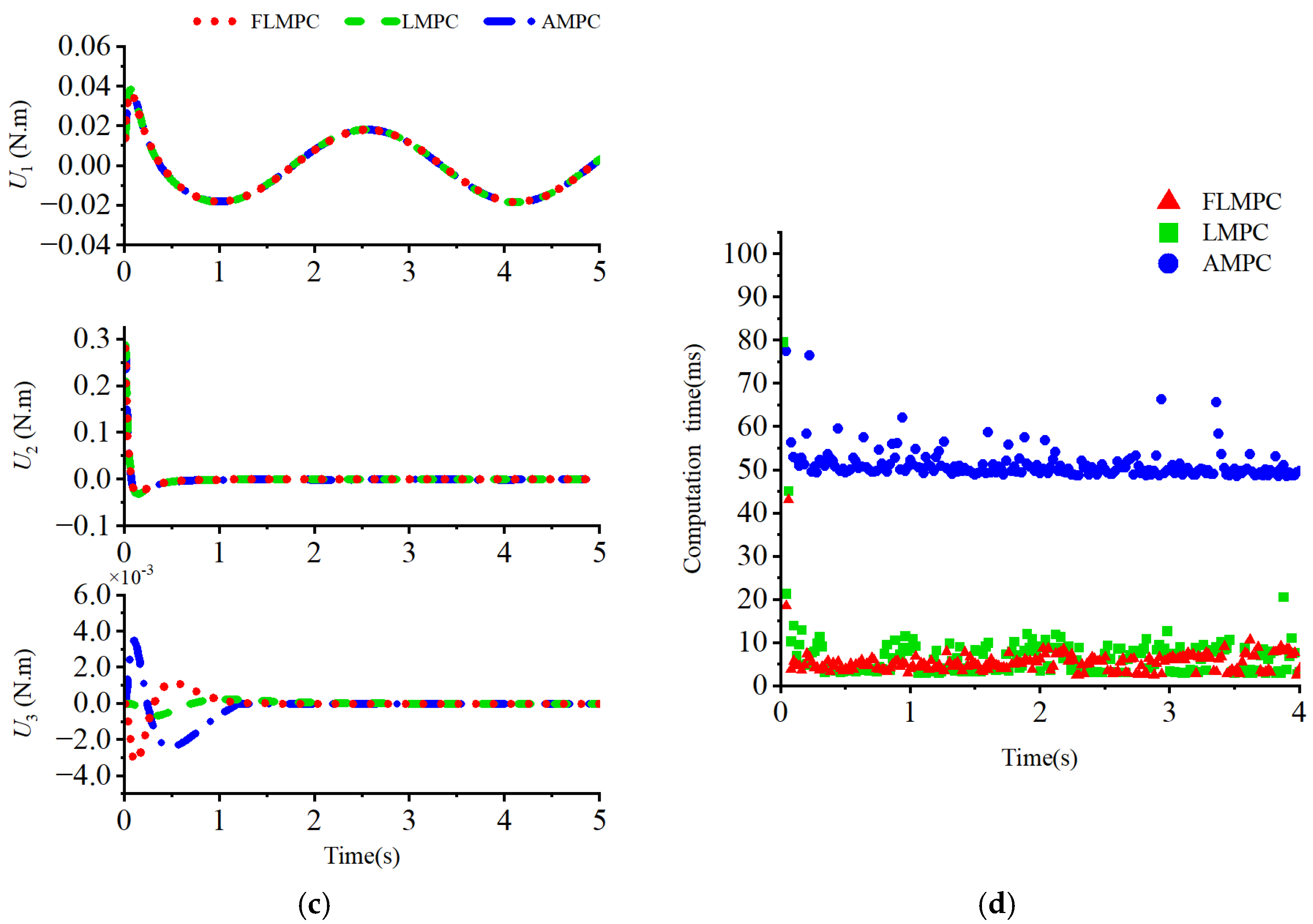
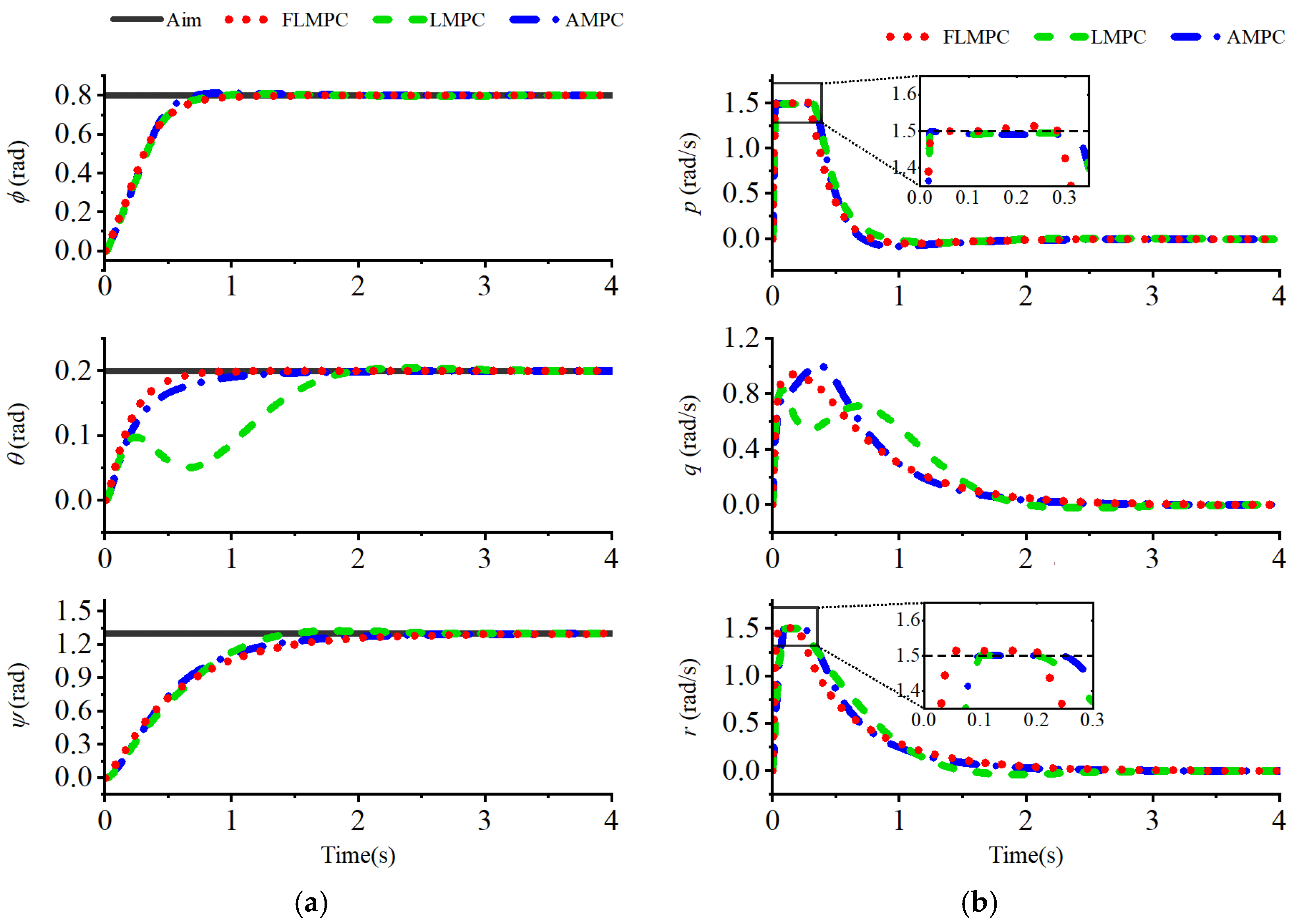
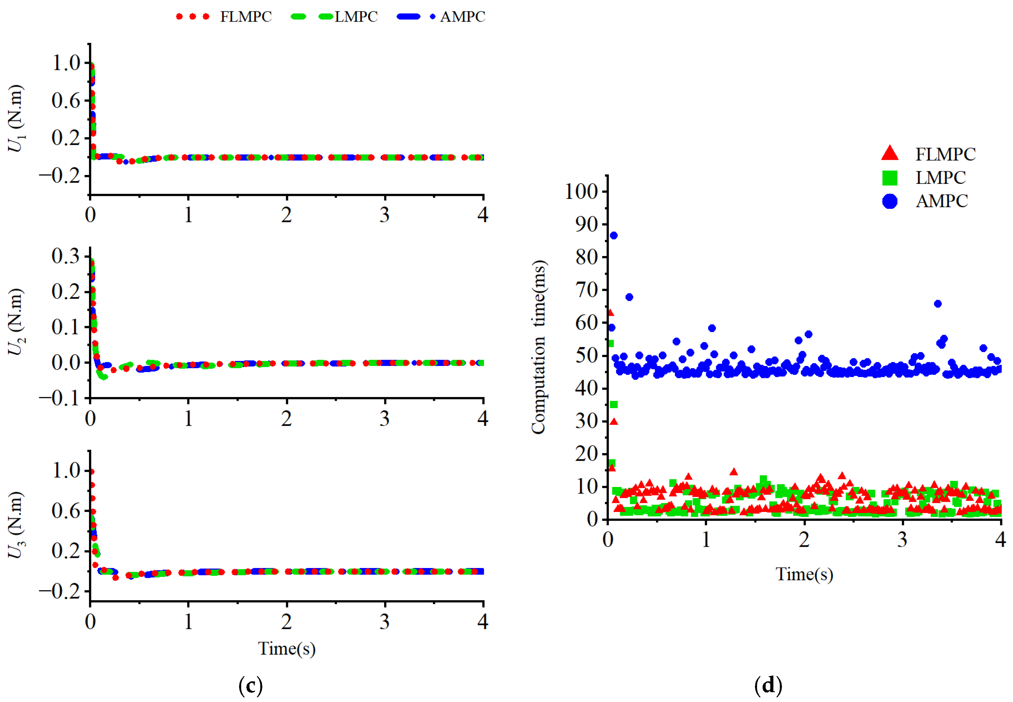
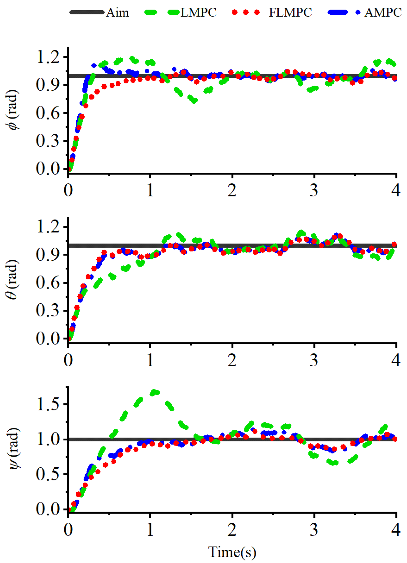
4.2. Results
4.3. Discussion
5. Conclusions
Author Contributions
Funding
Institutional Review Board Statement
Informed Consent Statement
Data Availability Statement
Conflicts of Interest
Appendix A. Attitude Controller Design Based on MPC
References
- Li, B.; Wang, Y. An Enhanced Model Predictive Controller for Quadrotor Attitude Quick Adjustment with Input Constraints and Disturbances. Int. J. Control Autom. Syst. 2022, 20, 648–659. [Google Scholar] [CrossRef]
- Thusoo, R.; Jain, S.; Bangia, S. Quadrotors in the Present Era: A Review. Inf. Technol. Ind. 2021, 9, 164–178. [Google Scholar]
- Lei, B.; Wang, N.; Xu, P.; Song, G. New crack detection method for bridge inspection using UAV incorporating image processing. J. Aerosp. Eng. 2018, 31, 04018058. [Google Scholar] [CrossRef]
- Idrissi, M.; Annaz, F. Dynamic modelling and analysis of a quadrotor based on selected physical parameters. Int. J. Mech. Eng. Robot. Res. (IJMERR) 2020, 9, 784–790. [Google Scholar] [CrossRef]
- Li, C.; Wang, Y.; Yang, X. Adaptive fuzzy control of a quadrotor using disturbance observer. Aerosp. Sci. Technol. 2022, 128, 107784. [Google Scholar] [CrossRef]
- Roy, R.; Islam, M.; Sadman, N.; Mahmud, M.P.; Gupta, K.D.; Ahsan, M.M. A Review on Comparative Remarks, Performance Evaluation and Improvement Strategies of Quadrotor Controllers. Technologies 2021, 9, 37. [Google Scholar] [CrossRef]
- Hassan, S.; Ali, A.; Rafic, Y. A survey on quadrotors: Configurations, modeling and identification, control, collision avoidance, fault diagnosis and tolerant control. IEEE Aerosp. Electron. Syst. Mag. 2018, 33, 14–33. [Google Scholar]
- Sheta, A.; Braik, M.; Maddi, D.R.; Mahdy, A.; Aljahdali, S.; Turabieh, H. Optimization of PID Controller to Stabilize Quadcopter Movements Using Meta-Heuristic Search Algorithms. Appl. Sci. 2021, 11, 6492. [Google Scholar] [CrossRef]
- Al Tahtawi, A.R.; Yusuf, M. Low-cost quadrotor hardware design with PID control system as flight controller. Telecommun. Comput. Electron. Control 2019, 17, 1923–1930. [Google Scholar] [CrossRef]
- Mirtaba, M.; Jeddi, M.; Nikoofard, A.; Shirmohammadi, Z. Design and implementation of a low-complexity flight controller for a quadrotor UAV. Int. J. Dyn. Control 2023, 11, 689–700. [Google Scholar] [CrossRef]
- Qiao, Z.; Zhuang, K.; Zhao, T.; Xue, J.; Zhang, M.; Cui, S.; Gao, Y. Simulation of a Quadrotor under Linear Active Disturbance Rejection. Appl. Sci. 2022, 12, 12455. [Google Scholar] [CrossRef]
- Labbadi, M.; Cherkaoui, M. Robust Integral Terminal Sliding Mode Control for Quadrotor UAV with External Disturbances. Int. J. Aerosp. Eng. 2019, 2019, 2016416. [Google Scholar] [CrossRef]
- Pan, J.; Shao, B.; Xiong, J.; Zhang, Q. Attitude Control of Quadrotor UAVs Based on Adaptive Sliding Mode. Int. J. Control Autom. Syst. 2023, 21, 2698–2707. [Google Scholar] [CrossRef]
- Islam, M.; Okasha, M. A Comparative Study of PD, LQR and MPC on Quadrotor Using Quaternion Approach. In Proceedings of the 2019 7th International Conference on Mechatronics Engineering (ICOM), Putrajaya, Malaysia, 30–31 October 2019; pp. 1–6. [Google Scholar]
- Lopes, R.V.; Santana, P.H.R.Q.A.; Borges, G.; Ishihara, J. Model predictive control applied to tracking and attitude stabilization of a VTOL quadrotor aircraft. In Proceedings of the 21st International Congress of Mechanical Engineering, Natal, Brazil, 24–28 October 2011; pp. 176–185. [Google Scholar]
- Chikasha, P.N.; Dube, C. Adaptive Model Predictive Control of a Quadrotor. Ifac Pap. 2017, 50, 157–162. [Google Scholar] [CrossRef]
- Villarreal, O.J.G.; Rossiter, J.A.; Shin, H. Laguerre-based adaptive MPC for attitude stabilization of quad-rotor. In Proceedings of the 2018 UKACC 12th International Conference on Control (CONTROL), Sheffield, UK, 5–7 September 2018; pp. 360–365. [Google Scholar]
- Benotsmane, R.; Vásárhelyi, J. Towards Optimization of Energy Consumption of Tello Quad-Rotor with Mpc Model Implementation. Energies 2022, 15, 9207. [Google Scholar] [CrossRef]
- Murilo, A.; Lopes, R.V. Unified NMPC framework for attitude and position control for a VTOL UAV. Proc. Inst. Mech. Eng. Part I J. Syst. Control Eng. 2019, 233, 889–903. [Google Scholar] [CrossRef]
- Kuantama, E.; Tarca, I.; Tarca, R. Feedback linearization LQR control for quadcopter position tracking. In Proceedings of the 2018 5th International Conference on Control, Decision and Information Technologies (CoDIT), Thessaloniki, Greece, 10–13 April 2018; pp. 204–209. [Google Scholar]
- Kong, X.; Abdelbaky, M.A.; Liu, X.; Lee, K.Y. Stable feedback linearization-based economic MPC scheme for thermal power plant. Energy 2023, 268, 126658. [Google Scholar] [CrossRef]
- Te Braake, H.A.B.; Ayala Botto, M.; Sá da Costa, J.; van Can, H.J.L.; Verbruggen, H.B. Linear predictive control based on approximate input-output feedback linearisation. IEE Proc.-Control Theory Appl. 1999, 146, 295–300. [Google Scholar] [CrossRef]
- Ermeydan, A.; Kaba, A. Feedback linearization control of a quadrotor. In Proceedings of the 2021 5th International Symposium on Multidisciplinary Studies and Innovative Technologies (ISMSIT), Ankara, Turkey, 21–23 October 2021; pp. 287–290. [Google Scholar]
- Palunko, I.; Fierro, R. Adaptive control of a quadrotor with dynamic changes in the center of gravity. IFAC Proc. Vol. 2011, 44, 2626–2631. [Google Scholar] [CrossRef]
- Rahmat, M.F.; Eltayeb, A.; Basri, M.A.M. Adaptive feedback linearization controller for stabilization of quadrotor UAV. Int. J. Integr. Eng. 2020, 12, 1–17. [Google Scholar]
- Cai, Z.; Zhang, S.; Jing, X. Model predictive controller for quadcopter trajectory tracking based on feedback linearization. IEEE Access 2021, 9, 162909–162918. [Google Scholar] [CrossRef]
- Baek, J.; Jung, J. A Model-Free Control Scheme for Attitude Stabilization of Quadrotor Systems. Electronics 2020, 9, 1586. [Google Scholar] [CrossRef]
- Xiong, J.J.; Zheng, E.H. Position and attitude tracking control for a quadrotor UAV. ISA Trans. 2014, 53, 725–731. [Google Scholar] [CrossRef]
- Shen, S.; Xu, J. Attitude active disturbance rejection control of the quadrotor and its parameter tuning. Int. J. Aerosp. Eng. 2020, 2020, 8876177. [Google Scholar] [CrossRef]
- Rinaldi, M.; Primatesta, S.; Guglieri, G. A Comparative Study for Control of Quadrotor UAVs. Appl. Sci. 2023, 13, 3464. [Google Scholar] [CrossRef]
- Morato, M.M.; Normey-Rico, J.E.; Sename, O. Model predictive control design for linear parameter varying systems: A survey. Annu. Rev. Control 2020, 49, 64–80. [Google Scholar] [CrossRef]
- Okasha, M.; Kralev, J.; Islam, M. Design and Experimental Comparison of PID, LQR and MPC Stabilizing Controllers for Parrot Mambo Mini-Drone. Aerospace 2022, 9, 298. [Google Scholar] [CrossRef]


| Parameters | Values | Unit |
|---|---|---|
| m | 0.8 | kg |
| Ix | 9.7 × 10⁻³ | kg∙m2 |
| Iy | 9.7 × 10⁻³ | kg∙m2 |
| Iz | 1.7 × 10⁻² | kg∙m2 |
| l | 0.06 | m |
| g | 9.81 | m/s2 |
| Performance Metrics | Response Time (s) | Overshoot (%) | Mean Computation Time (ms) | ||||
|---|---|---|---|---|---|---|---|
| FLMPC | 0.83 | 0.95 | 2.07 | 0.46 | 0.00 | 0.01 | 6.03 |
| LMPC | 0.76 | 2.7 | 2.25 | 1.07 | 2.17 | 1.88 | 5.23 |
| AMPC | 0.63 | 1.65 | 1.90 | 1.67 | 0.00 | 0.00 | 47.59 |
Disclaimer/Publisher’s Note: The statements, opinions and data contained in all publications are solely those of the individual author(s) and contributor(s) and not of MDPI and/or the editor(s). MDPI and/or the editor(s) disclaim responsibility for any injury to people or property resulting from any ideas, methods, instructions or products referred to in the content. |
© 2025 by the authors. Licensee MDPI, Basel, Switzerland. This article is an open access article distributed under the terms and conditions of the Creative Commons Attribution (CC BY) license (https://creativecommons.org/licenses/by/4.0/).
Share and Cite
Yuan, X.; Xu, J.; Li, S. Design and Simulation Verification of Model Predictive Attitude Control Based on Feedback Linearization for Quadrotor UAV. Appl. Sci. 2025, 15, 5218. https://doi.org/10.3390/app15095218
Yuan X, Xu J, Li S. Design and Simulation Verification of Model Predictive Attitude Control Based on Feedback Linearization for Quadrotor UAV. Applied Sciences. 2025; 15(9):5218. https://doi.org/10.3390/app15095218
Chicago/Turabian StyleYuan, Xingyu, Jinfa Xu, and Shengwei Li. 2025. "Design and Simulation Verification of Model Predictive Attitude Control Based on Feedback Linearization for Quadrotor UAV" Applied Sciences 15, no. 9: 5218. https://doi.org/10.3390/app15095218
APA StyleYuan, X., Xu, J., & Li, S. (2025). Design and Simulation Verification of Model Predictive Attitude Control Based on Feedback Linearization for Quadrotor UAV. Applied Sciences, 15(9), 5218. https://doi.org/10.3390/app15095218