Abstract
This research introduces a new method for creating synthetic Distributed Acoustic Sensing (DAS) datasets from transport microsimulation models. The process involves modeling detailed vehicle interactions, trajectories, and characteristics from the PTV VISSIM transport microsimulation tool. It then applies the Flamant–Boussinesq approximation to simulate the resulting ground deformation detected by virtual fiber-optic cables. These synthetic DAS signals serve as large-scale, scenario-controlled, labeled datasets on training machine learning models for various transport applications. We demonstrate this by training several U-Net convolutional neural networks to enhance spatial resolution (reducing it to half the original gauge length), filtering traffic signals by vehicle direction, and simulating the effects of alternative cable layouts. The methodology is tested using simulations of real road scenarios, featuring a fiber-optic cable buried along the westbound shoulder with sections deviating from the roadside. The U-Net models, trained solely on synthetic data, showed promising performance (e.g., validation MSE down to 0.0015 for directional filtering) and improved the detectability of faint signals, like bicycles among heavy vehicles, when applied to real DAS measurements from the test site. This framework uniquely integrates detailed traffic modeling with DAS physics, providing a novel tool to develop and evaluate DAS signal processing techniques, optimize cable layout deployments, and advance DAS applications in complex transportation monitoring scenarios. Creating such a procedure offers significant potential for advancing the application of DAS in transportation monitoring and smart city initiatives.
1. Introduction
Distributed Acoustic Sensing (DAS) technology transforms standard fiber-optic cables into dense arrays of virtual sensors capable of measuring dynamic strain rates along tens of kilometers with meter-scale spatial resolution. By analyzing Rayleigh backscattered light phase changes from laser pulses, DAS systems can detect vibrations along consecutive sections of the cable caused by nearby events. When deployed along transport networks, these systems sense ground deformations induced by passing vehicles (Figure 1), enabling long-range traffic monitoring with unique advantages in spatial coverage compared to traditional sensors.
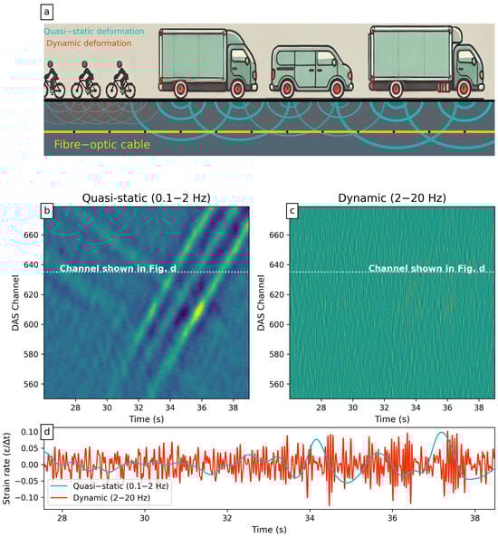
Figure 1.
Synoptic overview of real roadside DAS signal example from opposing traffic: three westbound lightweight vehicles (bicycles) crossing three heavy eastbound vehicles. (a) Vehicle weight causes quasi-static ground deformation (cyan), while tire–road interactions induce dynamic deformation (red). A buried fiber-optic cable (yellow) senses both. Black dots indicate approximate gauge length; (b) the quasi-static signals from the heavy vehicles produce trackable patterns over the DAS channels, while lighter vehicles are less distinct; (c) dynamic deformation is more complex, though its amplitude can be higher; (d) strain rate recording at one single DAS channel (white dotted line in (b,c).
While DAS has demonstrated value in geophysics and infrastructure monitoring [1,2,3], its application to traffic analysis still faces several challenges. The key challenges include achieving sufficient signal-to-noise ratio (SNR) and spatial resolution, especially in dense traffic, where heavier vehicles can mask lighter ones [4]. Existing methods using wavelet thresholds [5] and template matching [6] struggle in dense traffic scenarios and bidirectional flows, where signal overlaps from multiple vehicles degrade performance. Recent machine learning approaches [7] show promise but remain constrained by limited manually labeled datasets and the inability to model non-ideal cable layouts common in urban deployments.
Often, DAS deployment relies on existing “dark fiber” cable infrastructure near roads [8,9]. These pre-existing cable layouts may not be optimal for specific traffic monitoring tasks due to placement or distance variations. While potentially cost-effective for large networks [10], optimizing cable layout design can significantly improve detection [9]. Generating realistic synthetic DAS datasets is crucial not only for evaluating the benefit of potential custom cable layouts but also for developing robust signal processing algorithms before any field deployment.
Furthermore, most current techniques rely solely on point-specific real-world data collection [11], even if assisted with cameras [12], reducing their capacity to capture sufficiently diverse traffic scenarios and sensor configurations to generalize the analysis for long networks. Not having a balanced and sufficiently high number of examples for each type of vehicle, traffic condition, and cable/transport network combination can reduce the applicability of many processing techniques. The customization of the processing techniques relies on expensive data acquisition surveys, unless adequate synthetic data are produced.
Synthetic DAS analysis already exists in the seismology [8,13,14] but has only been used in specific traffic monitoring cases, such as [15], where synthetic labeled datasets were used to train machine learning (ML) models. By integrating synthetic dataset generation with transport models, we can create an unlimited supply of labeled data to support traffic agnostic data generalization for any specific network, regardless of the fine-tuning process that could be applied afterwards.
Our work addresses these limitations through a novel synthesis of transport microsimulation and physics-based modeling. Unlike prior DAS traffic studies that either use simplified vehicle models [9] or focus on post hoc analysis of field data [16], we integrate detailed vehicle trajectory simulations from PTV VISSIM with strain modeling via the Flamant–Boussinesq approximation (see Appendix A). This integration enables the generation of scenario-controlled synthetic datasets that are stochastically realistic and are customized for a given network. These datasets are able to capture complex interactions between the targeted vehicles, the fiber-optic cable geometry, and the subsurface response to the traffic dynamics—a capability absent in existing seismic-focused synthetic DAS frameworks [13,14].
The primary objective of this study is to introduce and validate a methodology for generating synthetic strain-rate signals simulating DAS measurements, derived from the outputs of transport microsimulation models.
Our secondary objectives are to demonstrate the framework’s utility by training ML models to perform critical tasks. The selected example applications target training (U-Net) models to enhance spatial resolution beyond hardware limitations (doubling the spatial resolution by reducing the effective gauge length from 1.034 m to 0.517 m), isolating directional traffic flows even for dense traffic situations and simulating the effects of alternative cable layouts. This approach aims to provide valuable tools for both the DAS and transport engineering communities to develop robust detection algorithms, optimize sensor deployments, and advance traffic analysis capabilities. Controlling dataset creation allows for various congestion levels under different cable layouts and complex traffic scenarios, ultimately contributing to advancements in traffic analysis and smart city initiatives utilizing DAS technology.
The methodology’s novelty lies in three key aspects:
- Transport–physics coupling: Direct mapping of microsimulated traffic and vehicle parameters (mass, wheelbase, driving behavior, acceleration, and speed profiles) to strain-rate signals through modeling. This reduces the label data acquisition costs for kilometer-scale networks while producing high numbers of labeled datasets for any targeted scenario across the whole transport network.
- Cable layout-aware synthesis: Explicit incorporation of real-world cable deployment factors like burial depth variations and non-linear routing. This enables the analysis of existing and future cable layouts.
- ML-ready datasets: Generation of paired synthetic measurements (features + labels) for supervised learning tasks, including directional filtering and resolution enhancement.
This paper is structured as follows: Section 2 details our synthetic signal generation pipeline, covering transport modeling and physics-based simulation. Section 3 outlines the machine learning implementation, and Section 4 presents the results, evaluating model performance on synthetic data and application to real DAS measurements. Section 5 addresses limitations and future directions for physics-informed DAS processing, while Section 6 summarizes the work and significance of the contribution. The appendices provide details on the Flamant–Boussinesq approximation (Appendix A) and the U-Net architecture (Appendix B).
2. Synthetic DAS Signal Generation Methodology
Generating realistic synthetic strain-rate signals simulating DAS measurements requires integrating detailed transport system modeling with physics-based simulation of ground deformation and sensor response. The overall workflow is depicted in Figure 2.
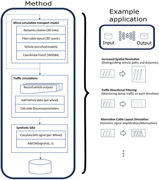
Figure 2.
Block diagram of the methodology to generate synthetic signals simulating DAS measurements from transport models, and example applications.
2.1. Transport Microsimulation (PTV VISSIM)
Microscopic transport models simulate individual vehicle movements and interactions within a defined network. We utilize PTV VISSIM for its detailed modeling capabilities. The key steps tailored for generating DAS-relevant inputs include the following:
- Network Creation: Define the road network links with 3D coordinates (including heights/gradients) and relevant attributes (lanes, speed limits, etc.). Include geophysical parameters (Poisson’s ratio , Young’s modulus E) as user-defined attributes for each link section to represent homogeneous ground conditions. Define traffic control elements (signals and signs) realistically.
- Fiber Layout Codification: Precisely define the 3D coordinates of the existing or desired fiber-optic cable layout relative to the transport network. This is crucial for calculating load effects. In VISSIM, this can be modeled as a non-traffic link chain (Figure 5).
- Vehicle Parameter Enrichment: Define the vehicle mix, including types relevant to DAS (cars, trucks, bicycles, etc.). Use the Heavy Good Vehicle class to define all vehicles in order to be able to assign a weight distribution to each type. Crucially, enrich standard VISSIM vehicle models with DAS-significant parameters: number of axles/wheels, wheelbase, track width, wheel positions relative to vehicle front, and estimated load percentage per wheel. This allows calculating the position and load of each wheel, even for vehicle types where VISSIM’s default axle representation is insufficient.
- Coordinate Transformation: Convert VISSIM’s internal coordinates to a global system like WGS 84 (latitude, longitude, and altitude) using user-defined attributes and scripts. This facilitates calculating distances between vehicle wheels and fiber segments consistently (code available; see page 17).
- Simulation Runs: Execute simulations with varying traffic densities (e.g., low, intermediate, and high flows) and random seeds to generate diverse scenarios. Set an appropriate simulation time step (e.g., 0.1 ).
Data Extraction and Preparation: The simulation output provides vehicle trajectories (positions over time) along with their enriched characteristics (wheel loads, dimensions) and associated link geophysical properties. Combine simulation results with vehicle type details (mass, wheel configuration). Calculate the perpendicular distance (y) from each wheel to the nearest point on the fiber-optic cable, as well as the distance along the fiber (x) from a reference start point to that nearest point, for each timestamp. This prepared dataset serves as input for the physics-based signal modeling.
2.2. Physics-Based Signal Modeling (Flamant–Boussinesq)
The ground deformation caused by a vehicle wheel’s static load is simulated using the Flamant–Boussinesq approximation ([17], Appendix A). This model calculates the displacement field in an elastic, homogeneous, isotropic semi-infinite half-space due to a normal point load on the surface. Given the typically slow speeds of vehicles relative to seismic wave velocities, this quasi-static approximation is considered valid for low-frequency traffic-induced strain.
The displacement () parallel to the fiber axis at a point () relative to the load, where y is the perpendicular distance and z is the burial depth, is given by the following (derived from Equations (A1) and (A2) in Appendix A):
where m is the mass per wheel, g is gravity, E is Young’s modulus, is Poisson’s ratio, and is the distance from the load.
The strain rate () measured by a DAS system over a gauge length L is approximated by the finite difference of the time derivative of the displacement at the ends of the gauge length:
where is the time derivative of , calculated numerically from the sequence of displacements as the vehicle moves. The total signal at a given channel (centered at x) is the superposition of the strain rates induced by all wheels of all vehicles at that time.
Assumptions and Limitations: The model assumes that the vehicle speeds are much smaller that the ground Rayleigh wave deformation velocity, therefore assuming a quasi-static deformation. Assuming dominance of static over dynamic tire–road interactions; see Figure 1 (justified by low-frequency DAS signals, see [7,11]). Another assumption derived from the Flamant–Boussinesq model is that the terrain is considered a perfectly elastic, homogeneous, and isotropic medium, which is a simplification of real ground conditions. It neglects dynamic effects, layering, and anisotropy. Pathological singularities can occur near the load, especially if the depth z is very small compared to y (Appendix A). For the typical depths (0.4 m) and distances in road applications, the model generally produces consistent wavelet shapes (Figure 3). Also, the model inherently assumes uniform fiber sensitivity and coupling along its different sections. Even though, for the case study, constant sensitivity and coupling characteristics were assumed, the methodology accounts for the possibility of including variations across variable-length sections. Variations in real-world installations (i.e., due to burial depth or pavement/soil compaction) can affect the signals and are not studied in the examples; this is a known limitation discussed further in Section 5.
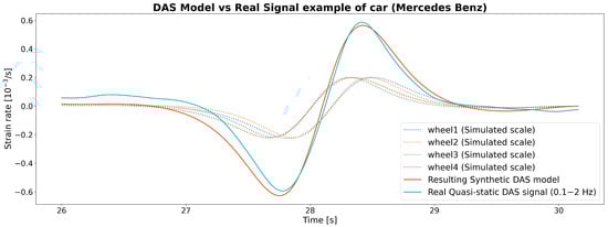
Figure 3.
Comparison of a real DAS signal corresponding to a light vehicle (Mercedes Class B) and the synthetic strain-rate signal simulating the DAS measurement for the same car model, created by combining the point load effects of each wheel using the Flamant–Boussinesq approximation.
2.3. Synthetic Dataset Creation
The synthetic strain-rate signals simulating DAS measurements are generated by applying Equations (1) and (2) for each wheel of each vehicle trajectory obtained from the VISSIM simulations (Section 2.1). The contributions from all wheels are summed at each DAS channel location and time step.
This process yields time-series data representing the strain rate along the virtual fiber for the simulated traffic scenario. To enhance realism for machine learning training, controlled noise (e.g., white noise with a specified standard deviation) can be added to the generated synthetic signals. This procedure allows the creation of large-scale, labeled datasets where the ground truth (e.g., vehicle type, direction, position, ideal signal from an alternative layout) is precisely known, facilitating the development and evaluation of DAS signal processing algorithms. Throughout this paper, the term “synthetic DAS signal” or “synthetic strain-rate signal” refers to this simulated output.
3. Experimental Design and Case Study
To demonstrate the methodology’s utility, we designed experiments using synthetic data to train machine learning models for specific transport monitoring tasks.
3.1. Objectives
The experiments aimed to showcase the framework’s capability to
- Generate large, labeled synthetic datasets representing various traffic conditions and sensor configurations.
- Train U-Net models using this synthetic data to perform tasks relevant to DAS traffic monitoring:
- -
- Enhancing spatial resolution beyond the instrument’s native gauge length.
- -
- Filtering traffic signals based on direction of travel.
- -
- Simulating the DAS response of alternative, potentially optimal, fiber-optic cable layouts.
- Evaluate the transferability of models trained purely on synthetic data to real DAS measurements.
3.2. Case Study: NA-150 Road
We selected a section of the NA-150 road in Navarra, Spain, as our case study (Figure 4). This is a two-lane interurban road with generally low traffic density. Crucially, a spare dark fiber-optic cable exists, buried approximately 40 cm deep in the shoulder along the westbound side.
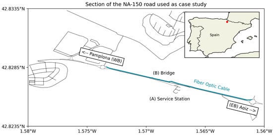
Figure 4.
Section of the Geographical location of the road NA-150 (red) layout and approximate fiber-optic cable location at westbound shoulder (cyan).
The chosen 1 km section includes features that challenge DAS measurements (Figure 5):
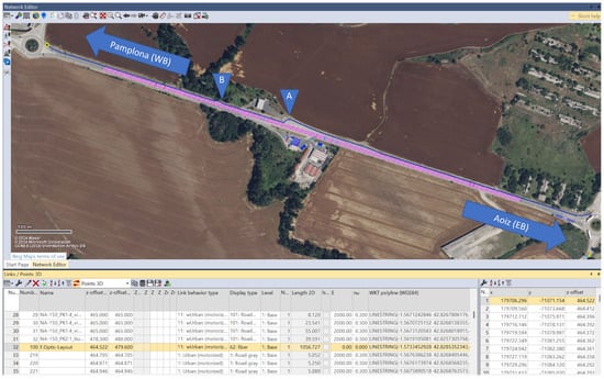
Figure 5.
VISSIM Micro-Transport model of the NA-150 road section. Road links are shown with lane markings. The blue line represents the codified fiber-optic cable path in the westbound shoulder, including depth and diversions at (A) the abandoned service station area and (B) the bridge.
- Strip A (Abandoned Service Station): The cable deviates significantly from the road shoulder, following the path of an old access lane. This increases the distance (y) to vehicles on the main road, weakening the signal.
- Strip B (Urbi River Bridge): The cable runs through a side conduit on the bridge, rather than being buried beneath the pavement. This alters the vibrational coupling compared to the buried sections.
These features provide opportunities to test the methodology’s ability to model and potentially compensate for non-ideal layouts. Real DAS data collected from this fiber using a differential-phase coherent optical time-domain reflectometry (COTDR) interrogator [18] were used for comparison and validation of the models trained on synthetic data.
The VISSIM model for this section was created as described in Section 2.1, incorporating the 3D road geometry, the detailed fiber path (including depth and deviations at A and B), and enriched vehicle types (cars, trucks, motorbikes, bicycles) with appropriate weights and dimensions. Simulations were run for 10 h each at low (50 veh./h/lane), intermediate (250 veh./h/lane), and high (500 veh./h/lane) traffic densities, generating trajectories for 998, 6162, and 10,070 vehicles, respectively.
3.3. Machine Learning Approach (U-Net)
We employed a U-Net convolutional neural network architecture (Appendix B), known for its effectiveness in image segmentation and processing tasks involving spatial context, which is relevant to DAS data (waterfall plots). The U-Net consists of an encoder path (down-sampling) to capture context and a symmetric decoder path (up-sampling) to enable precise localization, with skip connections linking corresponding encoder/decoder levels.
Our implementation used three encoder/decoder blocks with filter numbers {128, 256, 512} and a bridge with 1024 filters. The input to the network was a segment of synthetic DAS data (representing the “measured” signal), and the output was the corresponding “target” synthetic signal (e.g., higher resolution, filtered, or alternative layout). To achieve resolution enhancement, the target label datasets were generated at double the spatial resolution of the input feature datasets.
The input data were structured as strips covering the full fiber length (960 channels, gauge length ) over a temporal window of 6.4 s (64 time samples at 10 Hz). The target labels had 1920 channels ().
Training used the combined synthetic datasets from all three traffic densities. The data were split into 75% training and 25% validation. The training parameters were as follows: Adam optimizer, MSE loss, learning rate 0.001, batch size 8, and max 100 epochs with early stopping (patience 6).
Experiments Conducted: Separate U-Net models were trained for three distinct tasks, using specifically prepared synthetic feature/label pairs:
- Westbound (WB) Filtering and Resolution Enhancement:
- Feature Input: Synthetic signal (960 ch) from all traffic, using the actual WB shoulder layout (incl. Strips A/B), with added noise (std = 0.005).
- Label Output: Synthetic signal (1920 ch) containing *only* WB traffic, using the actual WB shoulder layout, with no added noise.
- Eastbound (EB) Filtering, Resolution Enhancement and Alternative Layout:
- Feature Input: Same as the WB experiment.
- Label Output: Synthetic signal (1920 ch) containing *only* EB traffic, simulating a hypothetical straight cable layout on the *eastbound* shoulder (no Strips A/B), with no added noise.
- Middle-of-Lane (MID) Layout Simulation and Resolution Enhancement:
- Feature Input: Same as the WB experiment.
- Label Output: Synthetic signal (1920 ch) containing *all* traffic (WB+EB), simulating a hypothetical straight cable layout placed in the *middle* of the roadway (between lanes), with no added noise.
These experiments test the model’s ability to learn complex transformations involving spatial upscaling, directional filtering, and geometric compensation based purely on synthetic examples.
4. Results
This section presents the performance evaluation of the U-Net models trained on synthetic data, first through validation on held-out synthetic datasets (Section 4.1) and subsequently by applying the trained models to real DAS measurements from the NA-150 road section (Section 4.2).
4.1. Performance on Synthetic Data (Validation)
The U-Net models were trained and validated using the synthetic datasets generated as described in Section 2 and Section 3. The objective was to quantitatively and qualitatively assess their ability to perform the three target tasks (resolution enhancement, directional filtering, layout simulation) within the controlled synthetic domain.
- Quantitative Evaluation: Validation performance was measured using mean squared error (MSE) and mean absolute error (MAE) between the model outputs and the target synthetic “label” datasets. The key results for models trained on the combined traffic density datasets with added input noise (std = 0.005) are summarized in Table A2 (from Appendix B).
- -
- Westbound (WB) Filtering and Resolution Enhancement: Achieved the lowest error (validation MSE = 0.0015, MAE = 0.0119), indicating high fidelity in isolating WB traffic and upscaling resolution while preserving the original layout’s characteristics.
- -
- Eastbound (EB) Filtering, Resolution Enhancement, and Alternative Layout: Showed significantly higher error (MSE = 0.1899, MAE = 0.0460). This reflects the increased complexity of simultaneously filtering EB traffic and transforming the signal to simulate a different cable path (straight EB shoulder).
- -
- Middle-of-Lane (MID) Layout Simulation and Resolution Enhancement: Also had considerable error (MSE = 0.1350, MAE = 0.0521), indicating the challenge of transforming signals from the WB shoulder layout (with diversions) to simulate a mid-road layout while processing traffic from both directions and balancing amplitudes.
- Observed Improvements: Visual inspection of the processed synthetic data confirms the intended effects (See Figure 6).
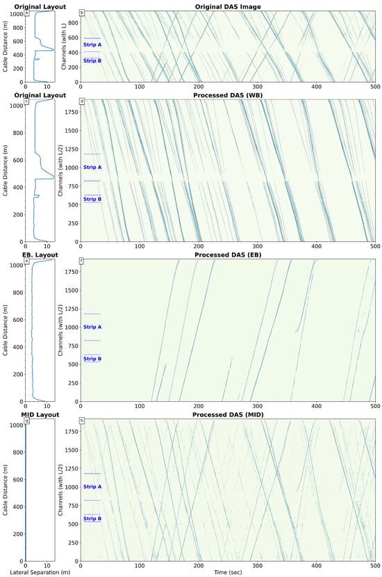 Figure 6. Synthetic DAS experiments. Column 1 (a,c,e,g) shows cable distance correspondent to the DAS channels vs. the lateral separation of the cable from road centerline, for different cable layouts: (a,c) original WB shoulder layout, (e) target EB shoulder layout, and (g) target MID-road layout. Column 2 (b,d,f,h) shows corresponding synthetic strain-rate signals (waterfall plots). (b) Input signal (960 ch) showing all traffic and effects of Strips A and B (with higher cable lateral separation due to the Abandoned Service Station and the Urbi River Bridge, respectively). (d,f,h) Processed outputs (1920 ch) with enhanced resolution: (d) WB-filtered result (original layout), (f) EB-filtered result (simulating EB layout, note absence of Strip A/B effects), and (h) all-traffic result (simulating MID layout, compensated for A/B). Sharpness of traces is compared in (d,f,h) vs. (b).
- -
- Spatial Resolution Enhancement: All models successfully doubled the spatial resolution from 1.034m (960 ch, Figure 6b) to 0.517 m (1920 ch, Figure 6d,f,h). This results in visually sharper and more distinct vehicle traces, potentially improving downstream tasks like vehicle counting or headway estimation.
- -
- -
- Layout Transformation: The EB model (Figure 6f) successfully compensated for the signal loss/distortion in Strips A and B, producing a signal consistent with the target straight EB shoulder layout (compare with Figure 6e). The MID model (Figure 6h) similarly compensated for Strips A and B and attempted to balance signal amplitudes between WB and EB traffic, consistent with the target mid-road layout (Figure 6g).
- Interpretation: The quantitative metrics validate U-Net’s ability to learn the desired transformations from synthetic data. The low MSE for the WB task demonstrates high accuracy when the target preserves the original layout geometry. The higher errors for the EB and MID tasks highlight the increased difficulty of learning complex transformations involving significant spatial extrapolation (simulating different cable positions) and amplitude re-balancing. Nonetheless, the visual results confirm that the models learned the intended filtering and layout simulation effects within the synthetic environment.
4.2. Application to Real DAS Data
To evaluate real-world applicability, the U-Net models, trained *exclusively* on the synthetic datasets, were applied to actual DAS measurements from the NA-150 test site. These real measurements (Figure 7b) contain signals from mixed traffic (including faint bicycle signals), real-world noise, and the true effects of the cable layout (Strips A/B).
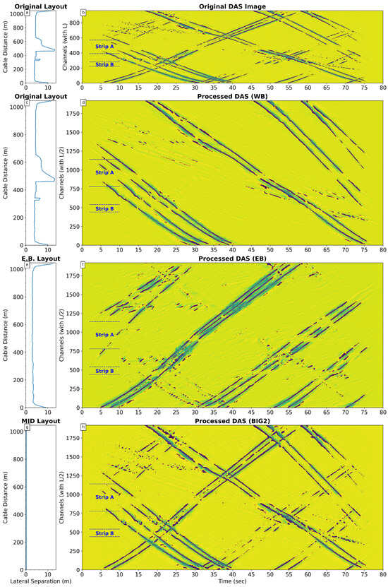
Figure 7.
Application to real DAS measurements. Column 1 (a,c,e,g) shows cable distance to road centerline (same as Figure 6). Column 2 (b,d,f,h) shows real DAS data (waterfall plots). (b) Input real DAS signal (960 ch), showing WB bicycles (faint, slow traces), heavier EB vehicles (stronger, faster traces), and effects of Strips A and B. (d, f, h) Processed outputs (1920 ch) from models trained on synthetic data: (d) WB-filtered result, enhancing bicycles; (f) EB-filtered result (simulating EB layout); (h) all-traffic result (simulating MID layout), notably enhancing bicycle visibility. Overall noise level and clarity are compared in (d,f,h) vs. (b).
- Observed Outcomes: The models successfully processed the real data, applying the learned transformations (see Figure 7 and Figure 8).
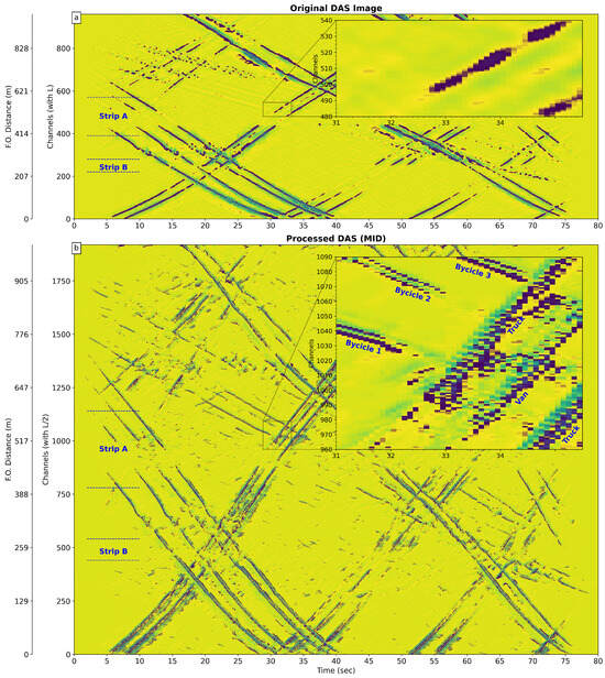 Figure 8. Zoomed comparison within Strip A (poor signal area due to cable diversion) between (a) input real DAS signal and (b) MID processed output. The faint signals from three westbound bicycles crossing paths with three eastbound heavy vehicles are barely visible in (a) but become significantly clearer and more distinct after processing in (b), despite the amplification of background noise.
- -
- Feature Enhancement: All models produced outputs with visually enhanced spatial resolution compared to the input. Notably, the MID model output (Figure 7h) significantly improved the visibility of the weak signals from a group of westbound bicycles traveling alongside heavier eastbound traffic. This enhancement is particularly striking in the challenging Strip A region (zoomed comparison in Figure 8), where the original signal (Figure 8a) is noisy and the bicycles are barely discernible, but they become much clearer in the processed output (Figure 8b).
- -
- Directional Filtering: The WB model (Figure 7d) demonstrated reasonable suppression of strong eastbound vehicle signals while enhancing westbound signals (including the bicycles). The EB model (Figure 7f) isolated eastbound traffic, though visual inspection suggests the filtering might be less clean than the WB result, with some potential residual WB signal.
- -
- Layout Simulation Effects: The outputs reflected the target layout characteristics learned from synthetic data. The EB model output (Figure 7f) shows reduced signal degradation in Strips A and B compared to the input (Figure 7b), consistent with simulating the straight EB shoulder layout. The MID model output (Figure 7h) appears to balance the amplitudes between the closer WB vehicles and the farther EB vehicles, as expected from simulating a mid-road position.
- Quantitative Comparison Limitations: Objective quantitative evaluation (MSE, PSNR, etc.) against a ground truth is not feasible for the real data application, as no “ideal” high-resolution, perfectly filtered real measurement exists. Performance assessment relies primarily on qualitative visual inspection and consistency checks against known events (e.g., the presence and direction of the bicycles and heavy vehicles).
- Performance Gap and Limitations (Synthetic vs. Real): Applying the synthetic-trained models to real data revealed key differences and limitations compared to the performance on synthetic validation data:
- -
- Noise Amplification: A major observed difference was the significant amplification of background noise in all processed real data outputs (clearly visible in Figure 7d,f,h and Figure 8b compared to Figure 7b and Figure 8a). While target features like bicycles were enhanced, the overall SNR appeared degraded. This strongly indicates that the simple additive white noise model used during synthetic training (std = 0.005) failed to capture the complex structure and characteristics of real-world DAS noise.
- -
- Artifacts and Imperfect Filtering: Some low-level artifacts and residual signals from the suppressed direction were visually apparent in the filtered outputs (e.g., faint diagonal traces potentially corresponding to strong EB vehicles in the WB-filtered output, Figure 7d). This suggests the filtering transformation learned on synthetic data did not perfectly generalize to the complexities of real signals.
- -
- Sensitivity to Calibration/Modeling Discrepancies: Imperfect modeling of the exact cable position, depth, coupling variations, and geophysical parameters likely contributes to the performance gap. Small errors in these aspects can lead to mismatches between the synthetic training examples and the real signal characteristics, limiting the model’s accuracy (discussed further in Section 5).
- Interpretation: Despite the limitations, applying the synthetically trained models to real DAS data demonstrated a relevant transfer of capabilities. The models successfully applied learned transformations like spatial resolution enhancement and directional filtering, notably improving the detectability of challenging weak signals (bicycles) even in areas of poor coupling (Strip A). This underscores the potential of using synthetic data for training pre-processing tools. However, the results also clearly highlight the challenge of the domain gap between the idealized synthetic training environment (simplified physics, basic noise) and the complex real-world sensing conditions. The noise amplification and imperfect filtering are key indicators of this gap and point to necessary future improvements in the synthetic data generation process, particularly regarding noise modeling.
5. Discussion
The framework presented successfully integrates transport microsimulation (VISSIM) with physics-based modeling (Flamant–Boussinesq) to generate synthetic strain-rate datasets simulating DAS measurements under diverse traffic conditions. The results demonstrate the potential of using these synthetic datasets to train machine learning models (U-Nets) for tasks like spatial resolution enhancement, directional filtering, and virtual sensor relocation (layout simulation).
The validation on synthetic data (Section 4.1) showed that the U-Net models could learn the target transformations with high fidelity when the task complexity was lower (e.g., WB filtering with original layout). Increased complexity, particularly involving simulating significant changes in cable geometry (EB and MID layouts), led to higher quantitative errors, suggesting limitations in the model’s ability to perfectly extrapolate signals under large spatial transformations based solely on the provided examples. Nevertheless, visually, the intended effects were achieved in the synthetic domain.
The application to real DAS data (Section 4.2) provided critical insights into the methodology’s practical applicability and current limitations. The successful enhancement of faint bicycle signals, especially in the challenging Strip A region, highlights a key benefit: using synthetic data to train models can improve the detection of difficult-to-observe events in real measurements. This “transposition of intended benefits” from synthetic training to real-world application is a promising outcome.
However, the significant amplification of background noise and the presence of filtering artifacts clearly expose the domain gap between the current synthetic data generation process and real-world DAS signals. The primary limitation appears to be the simplistic noise model (additive white noise). Real DAS noise is far more complex, potentially exhibiting frequency dependence, spatial correlations, and influences from environmental factors (temperature, terrain characteristics) and infrastructure vibrations not related to traffic. Future work must incorporate more sophisticated, data-driven noise models derived from spectral analysis of real background DAS measurements (periods without traffic) to improve the realism of the synthetic training data and reduce noise amplification upon real-world application.
Data standardization methods also warrant further investigation. While mean/variance scaling was used for synthetic data, the high dynamic range of DAS signals (heavy vs. light vehicles) might benefit from robust scaling methods (e.g., based on median and interquartile range), as was used for the real data input. Consistent and appropriate scaling across training and application is crucial.
Another key limitation is the accuracy of the input models—both the transport model and the physical model. Discrepancies between the modeled and actual fiber-optic cable path (including exact 3D position, potential slack in manholes causing channel misalignments between features like Strip A and Strip B), variations in burial depth and coupling efficiency, and inaccuracies in the assumed geophysical parameters (E, ) all contribute to mismatches between synthetic and real signals. Addressing this requires careful calibration. Incorporating ground truth data from controlled vehicle passes (with precise GPS tracking) could help calibrate the VISSIM model, geophysical parameters, and channel-to-location mapping.
The assumption of uniform fiber sensitivity and coupling inherent in the basic Flamant–Boussinesq model is another simplification. The real cable layout exhibits variations in response to the terrain and pavement characteristics along its length. While explicitly modeling this is complex, acknowledging it as a limitation is important. Future physical models could attempt to incorporate spatially varying coupling coefficients if calibration data allow.
Despite these limitations, the framework offers significant advantages. It provides a cost-effective, scalable, and controllable way to generate large volumes of labeled data for scenarios that might be rare or difficult to capture in real-world measurements. It allows systematic evaluation of different sensor layouts and processing techniques.
Future directions include the following:
- Developing more realistic noise models based on real DAS data analysis.
- Incorporating calibration data from controlled experiments to refine VISSIM parameters, geophysical properties, and channel mapping.
- Exploring more advanced physics-based models that account for dynamic effects, ground layering, or potentially non-uniform coupling.
- Extending the methodology to other transport modes (rail, pedestrians) or event types (incidents, road work).
6. Conclusions
This paper introduced and validated a novel methodology for generating synthetic strain-rate signals simulating Distributed Acoustic Sensing (DAS) measurements using outputs from transport microsimulation models (PTV VISSIM). By integrating detailed traffic modeling with physics-based ground deformation simulation (Flamant–Boussinesq), the framework provides a versatile tool for generating large-scale, labeled datasets representing diverse traffic scenarios and sensor configurations.
We demonstrated the utility of this approach by training U-Net models exclusively on synthetic data to perform key transport-based DAS signal processing tasks: enhancing spatial resolution, filtering traffic by direction, and simulating alternative fiber-optic cable layouts. Validation on synthetic data confirmed the models’ ability to learn these transformations. Application to real DAS measurements from the NA-150 road showed a relevant transfer of capabilities, notably enhancing the visibility of challenging faint signals (bicycles) even in areas with poor sensor coupling.
However, the application also highlighted limitations, primarily the domain gap between the current synthetic data (with simplified physics and noise models) and complex real-world signals, leading to noise amplification and imperfect filtering. Key areas for future improvement include developing more realistic noise models based on real data analysis and incorporating calibration procedures to refine model parameters and channel mapping. The inherent assumptions of the physical model (homogeneous medium, uniform coupling) also represent limitations to be addressed in future refinements.
Despite these areas for improvement, the proposed framework offers significant potential. It provides a cost-effective and controllable means to generate large labeled datasets for training and evaluating DAS processing algorithms, aids in optimizing sensor deployment strategies by simulating different layouts, and allows exploration of challenging traffic scenarios. This work bridges transport engineering and DAS sensing, contributing a valuable tool for advancing intelligent transportation systems and smart city monitoring initiatives by leveraging the unique capabilities of DAS technology. Continued development, particularly focusing on improved realism through better noise modeling and calibration, will further enhance the methodology’s impact.
Author Contributions
Conceptualization and methodology, I.R.-U.; software, I.R.-U., J.B., J.B.G. and P.D.G.; validation, I.R.-U., J.B., J.B.G. and P.D.G.; formal analysis, I.R.-U.; investigation, I.R.-U.; resources, A.C.; data curation, I.R.-U.; writing—original draft preparation, I.R.-U.; writing—review and editing, J.B., A.L., M.S., L.R.-C. and A.C.; visualization, I.R.-U.; supervision, L.R.-C. and A.C.; project administration, A.C.; funding acquisition, A.C. All authors have read and agreed to the published version of the manuscript.
Funding
This research was funded by the Spanish Goverment “Subprograma Ayudas Predoctorales 2020 Investigadores” program under Grant PRE2020-096336, assigned to the National Plan project PID2019-107270RB-C21, “Photonic Devices and Systems Sensors for Intelligent Structures and Non Destructive Evaluation I”; the National “Knowledge Generation Projects” project “Photonic Sensors for Smart and Sustainable Cities (Performance)” under grant ID6448137269-137269-4-22; the project “Integrated System for Traffic and Road Condition Monitoring Using Fiber-Optic Sensors (Ingestion)”, under grant PDC2021-121172-C22 funded by MICIU/AEI/10.13039/501100011033 and by the European Union Next GenerationEU/PRTR. This work was supported in part by grant PID2022-137269OB-C21 by MICIU/AEI/10.13039/501100011033 and by ERDF “A way of making Europe”; and grant PID2022-137269OB-C22 by MICIU/AEI/10.13039/501100011033 and by the European Union.
Institutional Review Board Statement
Not applicable.
Informed Consent Statement
Not applicable.
Data Availability Statement
The original PTV VISSIM configurations, U-Net training and validating scripts, models, and data presented in the study are openly available in ZENODO at DOI 10.5281/zenodo.15144354.
Acknowledgments
The authors would like to thank the reviewers for their constructive and insightful feedback. We would also like to express our sincere gratitude to PTV Group for their support and assistance with the microsimulation transport software tool, PTV VISSIM. This work was improved through beneficial discussions with Ignacio Galindo and Luca Manuel Vozzi. The authors also extend their appreciation to the SUM+LAB Research Group at Universidad de Cantabria for their constructive suggestions and guidance on transport models. Additionally, heartfelt thanks are due to the Institute of Smart Cities, Department of Electrical, Electronic, and Communications Engineering at Universidad Pública de Navarra, for enabling the evaluation of transport models using their DAS measurements. Finally, special recognition is given to the Photonics Engineering Group at Universidad de Cantabria, whose expertise, perspectives, and foundational support made the development of this work possible.
Conflicts of Interest
The authors declare no conflicts of interest. The funders had no role in the design of the study; in the collection, analyses, or interpretation of data; in the writing of the manuscript; or in the decision to publish the results.
Appendix A. The Flamant–Boussinesq Approximation
Appendix A.1. Mathematical Formulation
To predict the deformation of the ground in response to a vehicle’s weight, Jousset et al. [17] modeled it as a series of four point loads moving on an isotropic semi-infinite elastic half-space.
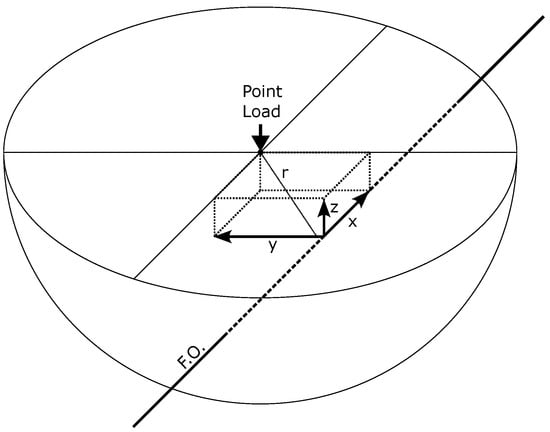
Figure A1.
Point load when applied on isotropic half-space along a fiber length (x), at depth (z), and with perpendicular separation (y).
Since the speed of the vehicle is slow compared to the Rayleigh wave velocity in the ground, the Flamant–Boussinesq approximation theory was used to describe the static deformation caused by a point load on the ground surface. According to this theory [19], the ground displacement in the ith direction is given by the following:
where
- is the particle displacement in the ith direction.
- F is the force of the point load (weight of the vehicle) applied on infinite half-space.
- is the shear modulus of the half-space.
- r is the distance from the origin and is given by .
- is the Kronecker sign (Einstein notation); assuming i ≠ j, then .
- is Poisson’s ratio.
If we assume the Kronecker sign to be 0 (when i ≠ j) and that , then we arrive at the next equation, as used by Van den Ende [20]:
where
- is the particle displacement in the x direction, defined parallel to the road (and the cable), at a point (y being the horizontal distance perpendicular to the road and z the depth beneath the surface) relative to the location of a point load positioned at the origin.
- z is the depth at which the fiber is buried with respect to the surface.
Equation (A2) describes the quasi-static deformation at a point in the subsurface caused by a series of point loads moving on an isotropic, semi-infinite elastic half-space. In this case, the Flamant–Boussinesq approximation can also be expressed based on Young’s modulus, since . Therefore arriving to Equation (1), where, the main parts are the same as the previous equation, except for the following:
- m: mass of the vehicle point load (mass per wheel).
- g: gravitational acceleration.
- E: Young’s elastic modulus of the road.
However, there are several assumptions made on these approximations that will limit the model’s use and application.
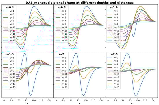
Figure A2.
Sensitivity analysis for the Flamant–Boussinesq shape form model of a wheel (monocycle) interacting with a cable at different depths and distances, where signal inversion appear for depths z and short lateral distances (y).
Appendix A.2. Limitations
In Boussinesq’s problem, a hypothetical concentrated load P acts at the origin of coordinates and is perpendicular to the plane surface of a semi-infinite solid. For our application, we consider the target to be a straight line buried at a specific depth below the surface.
The Flamant–Boussinesq approximation relies on several assumptions, the most important of which are as follows:
- Elastic, Homogeneous, Isotropic Medium: the soil is considered an elastic, homogeneous, isotropic, and semi-infinite medium.
- Linear Elasticity: the medium obeys Hooke’s law.
- No Self-Weight: the self-weight of the soil is ignored.
- Initial Stress: the soil is initially unstressed.
- Volume Change Neglect: the change in soil volume upon loading is neglected.
- Surface Conditions: the top surface is free of shear stress and subjected only to point loads.
- Stress Continuity: stress is continuous throughout the medium.
The application of the Boussinesq’s approximation applies easily on far-field domains and less so when describing the static deformation of a point loads located near the ground displacement, where the assumptions cannot be followed.
However, there are many cases in which the approximation is applied successfully on relatively low distances (see [6,9,17,20]), though most of the time with certain deep fibers (2 m [21]). According to Georgiadis ([22]), the behavior of the solutions near the point of application of the loads, where pathological singularities and discontinuities exist, is of particular importance. Studying these singularities and performing appropriate sensitivity analysis (see Figure A2 and Figure A3) reveals that for very shallow cables (z < 0.5 m), the result is a homogeneous down–up wavelet shape that attenuates with distance. However, for larger depths and shorter distances, there may be inversion changes in the shape (from up–down to down–up shapes).
For this approximation, the obtained waveforms will be on a continuous zone if a maximum shallow depth (z < 0.5 m) is maintained, or alternatively, if a minimum relative distance is ensured such that the depth component z has a value greater than or equal to the perpendicular separation component . In either of these two cases, adjusting the scale and sign will produce signals compatible with the observations.
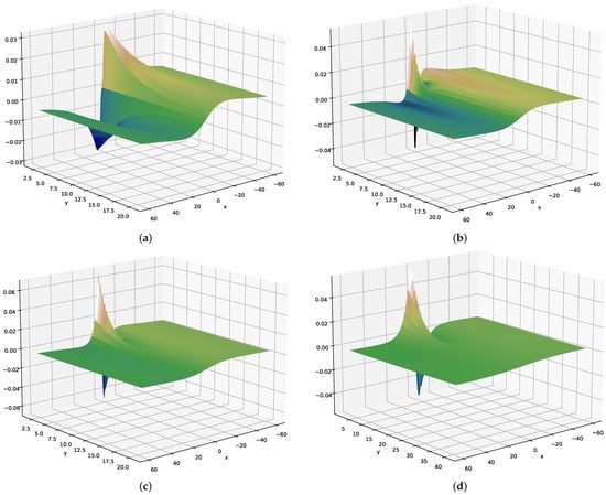
Figure A3.
Point Load Model sensitivity analysis along a fiber length (x), for different possible perpendicular separations (y), while the depth is (a) , (b) , (c) , and (d) .
Appendix A.3. Point Load Model for Different z
If we perform a sensitivity analysis where we draw the waveform of the Point Load Model along a fiber length (x), for different possible perpendicular separation (y), while the depth (z) varies, as indicated in Figure A3, we can observe how the waveform changes from a down–up configuration for shallow depths () to the highly attenuated up–down configuration for high values of z. For intermediate z values, the singularities make the waveform irregular.
Appendix B. Overview of U-Net-Based Autoencoder Architecture
The U-Net architecture used in the experiments was built using specific layer blocks described below:
- Convolution Block:
- Encoder Block:
- Decoder Block:
Encoder Path (Contraction Path): The encoder extracts features at different scales using convolutional layers and max-pooling operations to progressively reduce spatial dimensions. The encoder block is applied three times sequentially with 128, 256, and 512 filters, respectively. Each convolution block output (“x”) is stored for later concatenation in the decoder.
Bridge: The bridge connects the encoder and decoder paths by applying a convolution block with 1024 filters.
Decoder Path (Expansion Path): The decoder increases image resolution while combining features from encoder layers through concatenation. Similar to the encoder path, three decoder blocks are applied sequentially with 512, 256, and 128 filters, respectively.
Output Layer: The output layer consists of a convolution operation with a single filter of size , followed by a linear activation function for regression prediction:
- Summary of Network Architecture
- Encoder:
- Block 1: 128 filters → MaxPooling.
- Block 2: 256 filters → MaxPooling.
- Block 3: 512 filters → MaxPooling.
- Bridge: 1024 filters.
- Decoder:
- Block 1: 512 filters.
- Block 2: 256 filters.
- Block 3: 128 filters.
- Output: Convolutional layer with linear activation.
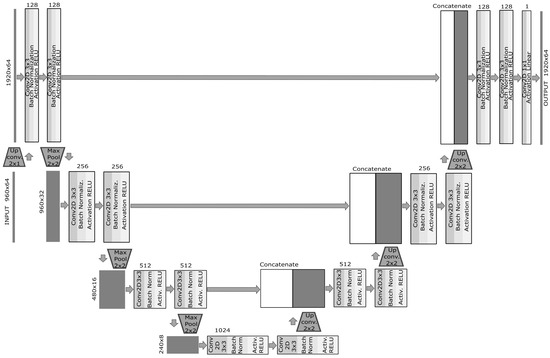
Figure A4.
UNET structure.
Training Metrics
To evaluate performance, the initial experiments focused solely on spatial resolution enhancement without introducing noise into the data. The model achieved a mean squared error of on the validation set after 93 epochs of training when using all the simulations. Examples showcasing these results are provided below.

Table A1.
Validation error metrics based on the datasets (initial experiments: resolution enhancement only, no added noise).
Table A1.
Validation error metrics based on the datasets (initial experiments: resolution enhancement only, no added noise).
| Traffic Dataset | Mean Absolute Error | Mean Squared Error | Root Mean Squared Error |
|---|---|---|---|
| (MAE) | (MSE) | (RMSE) | |
| Interm. density (6162 veh.) | 0.0363885 | 0.0094603 | 0.0972645 |
| Low density (998 veh.) | 0.0671135 | 0.0646277 | 0.2542198 |
| High density (10,070 veh.) | 0.0697876 | 0.0091005 | 0.0953966 |
| All (17,230 veh.) | 0.0318272 | 0.0081719 | 0.0903987 |
The next validation error metrics show the results when training the main experiments (WB, EB, MID) under dense traffic conditions and with random white noise added to the input features (std = 0.005).
Table A2.
Validation error metrics for main experiments (WB, EB, MID) with input noise (std = 0.005).
Table A2.
Validation error metrics for main experiments (WB, EB, MID) with input noise (std = 0.005).
| Experiment | Mean Absolute Error | Mean Squared Error | Root Mean Squared Error |
|---|---|---|---|
| (MAE) | (MSE) | (RMSE) | |
| Westbound (WB) direction | 0.0119055 | 0.0014845 | 0.0385295 |
| Eastbound (EB) direction | 0.0459715 | 0.1898927 | 0.4357668 |
| Middle (MID) direction | 0.0520504 | 0.1350333 | 0.3674688 |
References
- Cheng, F.; Chi, B.; Lindsey, N.; Dawe, T.; Ajo-Franklin, J. Utilizing distributed acoustic sensing and ocean bottom fiber optic cables for submarine structural characterization. Sci. Rep. 2021, 11, 5613. [Google Scholar] [CrossRef] [PubMed]
- Ajo-Franklin, J.; Dou, S.; Lindsey, N.; Monga, I.; Tracy, C.; Robertson, M.; Rodríguez Tribaldos, V.; Ulrich, C.; Freifeld, B.; Daley, T.; et al. Distributed Acoustic Sensing Using Dark Fiber for Near-Surface Characterization and Broadband Seismic Event Detection. Sci. Rep. 2019, 9, 1328. [Google Scholar] [CrossRef] [PubMed]
- Zhu, H.H.; Liu, W.; Wang, T.; Su, J.W.; Shi, B. Distributed Acoustic Sensing for Monitoring Linear Infrastructures: Current Status and Trends. Sensors 2022, 22, 7550. [Google Scholar] [CrossRef] [PubMed]
- Liu, J.; Li, H.; Yuan, S.; Noh, H.Y.; Biondi, B. Characterizing Vehicle-Induced Distributed Acoustic Sensing Signals for Accurate Urban Near-Surface Imaging. arXiv 2024, arXiv:2408.14320. [Google Scholar] [CrossRef]
- Liu, H.; Ma, J.; Yan, W.; Liu, W.; Zhang, X.; Li, C. Traffic Flow Detection Using Distributed Fiber Optic Acoustic Sensing. IEEE Access 2018, 6, 68968–68980. [Google Scholar] [CrossRef]
- Lindsey, N.J.; Yuan, S.; Lellouch, A.; Gualtieri, L.; Lecocq, T.; Biondi, B. City-Scale Dark Fiber DAS Measurements of Infrastructure Use During the COVID-19 Pandemic. Geophys. Res. Lett. 2020, 47, e2020GL089931. [Google Scholar] [CrossRef] [PubMed]
- van den Ende, M.; Ferrari, A.; Sladen, A.; Richard, C. Next-Generation Traffic Monitoring with Distributed Acoustic Sensing Arrays and Optimum Array Processing. In Proceedings of the 2021 55th Asilomar Conference on Signals, Systems, and Computers, Pacific Grove, CA, USA, 31 October–3 November 2021; pp. 1104–2303. [Google Scholar] [CrossRef]
- Luckie, T.; Porritt, R. Performance of synthetic DAS as a function of array geometry. Seismica 2024, 3, 2. [Google Scholar] [CrossRef]
- Yuan, S.; Lellouch, A.; Clapp, R.G.; Biondi, B. Near-surface characterization using a roadside distributed acoustic sensing array. Lead. Edge 2020, 39, 646–653. [Google Scholar] [CrossRef]
- Robles Urquijo, I.; Cobo García, A.; Cobo, L.R.; Quintela Incera, M. Real options of distributed DAS sensing applied to road transport engineering. Transp. Res. Procedia 2023, 71, 323–330. [Google Scholar] [CrossRef]
- Wang, H.; Chen, Y.; Min, R.; Chen, Y. Urban DAS Data Processing and Its Preliminary Application to City Traffic Monitoring. Sensors 2022, 22, 9976. [Google Scholar] [CrossRef] [PubMed]
- Cohen, K.; Hen, L.; Lellouch, A. Training a Distributed Acoustic Sensing Traffic Monitoring Network With Video Inputs. arXiv 2024, arXiv:2412.12743. [Google Scholar]
- Kennett, B.L.N. The seismic wavefield as seen by distributed acoustic sensing arrays: Local, regional and teleseismic sources. Proc. R. Soc. Math. Phys. Eng. Sci. 2022, 478, 20210812. [Google Scholar] [CrossRef] [PubMed]
- Zhai, Q.; Husker, A.; Zhan, Z.; Biondi, E.; Yin, J.; Civilini, F.; Costa, L. Assessing the feasibility of Distributed Acoustic Sensing (DAS) for moonquake detection. Earth Planet. Sci. Lett. 2024, 635, 118695. [Google Scholar] [CrossRef]
- Xie, D.; Wu, X.; Guo, Z.; Hong, H.; Wang, B.; Rong, Y. Intelligent Traffic Monitoring with Distributed Acoustic Sensing. arXiv 2024, arXiv:2403.02791. [Google Scholar] [CrossRef]
- Wiesmeyr, C.; Coronel, C.; Litzenberger, M.; Doller, H.J.; Schweiger, H.B.; Calbris, G. Distributed Acoustic Sensing for Vehicle Speed and Traffic Flow Estimation. In Proceedings of the 2021 IEEE International Intelligent Transportation Systems Conference (ITSC), Indianapolis, IN, USA, 19–22 September 2021. [Google Scholar] [CrossRef]
- Jousset, P.; Reinsch, T.; Ryberg, T.; Blanck, H.; Clarke, A.; Aghayev, R.; Hersir, G.P.; Henninges, J.; Weber, M.; Krawczyk, C.M. Dynamic strain determination using fibre-optic cables allows imaging of seismological and structural features. Nat. Commun. 2018, 9, 2509. [Google Scholar] [CrossRef] [PubMed]
- Corera, C.; Piñeiro Ben, E.; Navallas Irujo, J.; Sagüés García, M.; Loayssa Lara, A. Long-range traffic monitoring based on pulse-compression distributed acoustic sensing and advanced vehicle tracking and classification algorithm. Sensors 2023, 23, 3127. [Google Scholar] [CrossRef] [PubMed]
- Fung, Y.C. Foundations of Solid Mechanics; Springer: Berlin/Heidelberg, Germany, 1965. [Google Scholar]
- van den Ende, M.; Ferrari, A.; Sladen, A.; Richard, C. Deep Deconvolution for Traffic Analysis With Distributed Acoustic Sensing Data. IEEE Trans. Intell. Transp. Syst. 2023, 24, 2947–2962. [Google Scholar] [CrossRef]
- Yuan, S.; Ende, M.v.d.; Liu, J.; Noh, H.Y.; Clapp, R.; Richard, C.; Biondi, B. Spatial Deep Deconvolution U-Net for Traffic Analyses with Distributed Acoustic Sensing. IEEE Trans. Intell. Transp. Syst. 2022, 25, 1913–1924. [Google Scholar] [CrossRef]
- Georgiadis, H.G.; Anagnostou, D.S. Problems of the Flamant–Boussinesq and Kelvin Type in Dipolar Gradient Elasticity. J. Elast. 2007, 90, 71–98. [Google Scholar] [CrossRef]
Disclaimer/Publisher’s Note: The statements, opinions and data contained in all publications are solely those of the individual author(s) and contributor(s) and not of MDPI and/or the editor(s). MDPI and/or the editor(s) disclaim responsibility for any injury to people or property resulting from any ideas, methods, instructions or products referred to in the content. |
© 2025 by the authors. Licensee MDPI, Basel, Switzerland. This article is an open access article distributed under the terms and conditions of the Creative Commons Attribution (CC BY) license (https://creativecommons.org/licenses/by/4.0/).