Article

Multi-Module Combination for Underwater Image Enhancement

1
Shanghai Engineering Research Center of Hadal Science and Technology, College of Engineering Science and Technology, Shanghai Ocean University, Shanghai 201306, China
2
College of Oceanography, Zhejiang University, Zhejiang 316021, China
3
Shenzhen Institute for Advanced Study, University of Electronic Science and Technology of China, Shenzhen 518110, China
*
Author to whom correspondence should be addressed.
Appl. Sci. 2025, 15(9), 5200; https://doi.org/10.3390/app15095200
Submission received: 20 March 2025 / Revised: 1 May 2025 / Accepted: 5 May 2025 / Published: 7 May 2025

Abstract

:
Underwater observation and operation for divers and underwater robots still largely depend on optic methods, such as cameras videos, etc. However, due to the poor quality of images captured in murky waters, underwater operations in such areas are greatly hindered. In order to solve the issue of degraded images, this paper proposes a multi-module combination method (UMMC) for underwater image enhancement. This is a new solution for processing a single image. Specifically, the process consists of five modules. With five separate modules working in tandem, UMMC provides the flexibility to address key challenges such as color distortion, haze, and low contrast. The UMMC framework starts with a color deviation detection module that intelligently separates images with and without color deviation, followed by a color and white balance correction module to restore accurate color. Effective defogging is then performed using a rank-one prior matrix-based approach, while a reference curve transformation adaptively enhances the contrast. Finally, the fusion module combines the visibility and contrast functions with reference to two weights to produce clear and natural results. A large number of experimental results demonstrate the effectiveness of the method proposed in this paper, which shows good performance compared to existing algorithms, both on real and synthetic data.

1. Introduction

With profound changes in the global economic landscape and the in-depth promotion of the concept of sustainable development, the development of marine resources is gradually becoming a new strategic upper hand for which countries are competing. As an important tool for the exploitation of marine resources, marine engineering equipment requires a careful observation and analysis of the underwater environment at every stage, from its initial construction, mid-term maintenance and inspection to its later disassembly [1]. Marine resource surveys require high-resolution images to accurately observe seabed topography and resource distribution, thereby providing essential data support for marine development. Archeologists also rely on clear images to effectively identify and analyze underwater artifacts, which is critical for the protection of underwater cultural heritage in archeological research [2]. Furthermore, captured images are integral to various tasks, including underwater robot navigation, target tracking, and seabed environment monitoring. Underwater image enhancement is therefore essential and has extensive applications across multiple fields.
Underwater environments possess unique characteristics, such as low light levels, turbid water, and object reflections, which present significant challenges for the acquisition and processing of underwater images [3]. The imaging quality of underwater images is susceptible to complex hydrodynamic effects, which are mainly characterized by typical degradation features such as non-smooth noise interference, non-uniform optical blurring and multi-spectral attenuation [4]. Degraded features in underwater images can significantly reduce the localization accuracy of target detection, weaken the robustness of feature recognition, and lead to the accumulation of trajectory drift errors during dynamic tracking. By enhancing underwater images, the quality can be significantly improved, thereby increasing the reliability and utility of underwater vision systems. Underwater image enhancement, a crucial technology at the intersection of computer vision and marine optics, aims to reconstruct high-quality images with physical interpretability. This is achieved by establishing a mapping relationship between degradation models and visual perception, thereby overcoming the limitations imposed by complex underwater environments on the effectiveness of visual systems.
In response to the technical challenges presented by complex underwater imaging environments, researchers have proposed a range of innovative solutions in recent years. One such approach is a filter-based single-image defogging method that utilizes a guided joint bilateral filtering technique for haze removal [5]. The proposed algorithm excels in enhancing underwater images, achieving substantial improvements in both perceptual quality and objective evaluation metrics through effective contrast enhancement and noise suppression. Recent advances in deep learning have dramatically transformed underwater image enhancement methods, facilitating overall quality improvement through an end-to-end learning framework. In particular, the developed enhancement network is trained on a reference dataset and demonstrates exceptional capabilities in image processing [6]. Based on the insights gathered from our predecessors, we propose an architecture that first assesses whether to correct the image for color and white balance, depending on the outcomes of color deviation detection. Subsequently, it performs visibility restoration and contrast enhancement processes, followed by a fusion step to create an enhanced underwater image. Figure 1 illustrates the results of the visualization of the enhancement effect of this method in real and simulated underwater scenes in comparison. The main innovation of this study is reflected in the following dimensions:
  • In this paper, we present an algorithm that utilizes color bias detection to identify color bias in images. A white balance technique is then applied to process the color-biased images. This preprocessing step enhances the detection of color bias, thereby improving the accuracy of subsequent image processing tasks.
  • We employ a defogging and contrast enhancement algorithm that utilizes a rank-one prior matrix and curve transformation. The clarity and legibility of the underwater image are improved by converting it to the LAB color space, removing fog with the rank-one prior matrix, and enhancing the image’s contrast through a curve transformation.
  • The defogged image is combined with a contrast-enhanced image to produce a clearer and more recognizable underwater image.
The structure of this paper is organized as follows. Section 2 is an introduction to related work. Section 3 is divided into six subsections detailing the model structure of UMMC. Section 4 first describes the configuration of the experimental environment and then conducts three aspects of validation: (1) qualitative and quantitative evaluations on the UIEB and SUID datasets, (2) feature point matching experiments to verify the effectiveness of the enhanced images in improving the accuracy of underwater target recognition, and (3) an ablation study to assess the independent contributions of each technical component. Finally, an analysis of algorithm complexity and real-time testing are performed. Section 5 summarizes the research results and discusses future research directions.

2. Related Work

Underwater image enhancement represents a critical research area in marine science and technology, with significant contributions from numerous scholars aimed at facilitating more efficient and accurate ocean exploration.
Contrast Enhancement: Ding et al. [7] proposed a contrast enhancement fusion algorithm based on non-subsampled shearlet transform (NSST) framework. The method conducts a multiscale decomposition of the source image, separating it into low-frequency components and high-frequency sub-bands across multiple directions. Drawing on characteristics of human visual perception, the research team innovatively categorizes the low-frequency components into visually salient and non-salient regions. They effectively enhance the global contrast of the image through a fusion strategy while better preserving the detailed features of different regions. Zhang et al. [8] developed an innovative framework for underwater image enhancement that integrates color correction with dual-range contrast optimization. Their approach employs a sophisticated bi-interval histogram processing technique, which automatically determines an optimal equalization threshold to preserve a natural appearance while preventing over-enhancement. Additionally, the method incorporates an adaptive S-curve transformation to selectively boost local contrast and accentuate fine image details, achieving balanced enhancement across various regions of underwater images. In another study, Zhang et al. [9] tackled the issue of image degradation by implementing color channel correction and detail-preserving contrast enhancement. They designed a specialized attenuation matrix to compensate for inferior color channels.
Image Fusion: Xu et al. [10] designed a novel, unified, and unsupervised end-to-end image network to address various image fusion challenges. Zhang et al. [11] introduced a fast unified image fusion network based on the Proportional Maintenance of Gradients and Intensities (PMGI), which reformulates the image fusion problem as one of maintaining the proportionality of texture and intensity in the source images to accomplish multiple image fusion tasks. Tang et al. [12] developed a semantic-aware real-time image fusion network (SeAFusion) that integrates the image fusion module with a semantic segmentation module. Prince et al. [13] presented a multiple exposure image fusion method designed to merge bracketed exposure captures into a single image, enhancing details across a wide dynamic range.
Underwater Image Enhancement: Sudhanthira et al. [14] proposed a multi-module fusion image enhancement network that integrates the original weights of two images along with correlation weights during processing. Jiang et al. [15] proposed a dual-domain migration-based underwater image enhancement method, which achieves the robust migration of cross-domain features by constructing a progressive feature transformation mechanism from the airborne domain to the underwater domain. Zhou et al. [16] also achieved cross-domain adaptation from the aerial domain to the underwater domain by implementing a multi-feature enhancement mechanism (MFEF). This method utilizes multipath input to extract diverse forms of rich features from multiple viewpoints. Zhang et al. [17] developed a weighted wavelet visual perception fusion-based underwater image enhancement technique, which produces high-quality underwater images by merging high-frequency and low-frequency components from images of varying scales.
While deep learning solutions in existing research have achieved promising results, their performance often relies heavily on large-scale training datasets and substantial computational resources. Traditional methods, as a crucial component of underwater image enhancement research, warrant in-depth study. Building on previous solutions that address individual problems in underwater images, we are inspired to tackle multiple types of challenges in underwater environments through multi-module combination techniques. Therefore, we propose a multi-module combination technique for underwater image enhancement.

3. Proposed Method

This section outlines our methods for enhancing underwater images. First, we present the overall framework of the proposed enhancement technique. Subsequently, each module is described in detail.

3.1. Framework Architecture

Figure 2 illustrates the general framework of the UMMC method, which comprises five fundamental modules. The color deviation detection module is primarily designed for images exhibiting color deviations, although such deviations may not be readily apparent in shallow water images. The color and white balance correction module computes a nonlinear color mapping function to correct the image’s color by employing a k-nearest neighbor strategy. The visibility restoration module utilizes an enhanced rank-one a priori matrix decomposition technique, combined with depth information estimation, to achieve the precise removal of scattering blur [18]. The contrast enhancement module enhances the image’s brightness through grayscale correction and the probability distribution of brightness pixels while also applying gamma correction to automatically improve the image contrast. The image fusion module integrates images processed by the contrast enhancement module with those processed through multiple exposures.

3.2. Color Devviation Detection Module

In turbid water, deep water, or low-light environments, the scattering and wavelength attenuation of suspended particles can lead to color deviations. Different scenes are corrected using various color compensation methods to obtain high-quality underwater images. This process not only conserves computational resources by preventing the unnecessary processing of non-color-biased images, but it also ensures that certain images resemble terrestrial images due to the clarity of the seawater. The algorithm analyzes the features of the image by examining the digital image itself. Specifically, the texture information of the image is incorporated into the projection factor K [19]. A crucial step in detecting color deviation involves converting the input image from the RGB color space to the Lab color space. This conversion process begins by transforming the RGB data into the XYZ color space through a linear transformation, which serves as an intermediate step. The XYZ color space possesses device-independent characteristics, providing a standardized basis for color representation in the subsequent conversion. Once the XYZ values are obtained, the XYZ color space is mapped to the Lab color space through a nonlinear transformation. This mapping aligns more closely with the characteristics of human visual perception and facilitates the subsequent analysis of color deviation.
By analyzing both non-color and color images, Fang et al. [19] found that color bias is closely related to the mean and distribution characteristics of the image’s chromaticity. If the chromaticity distribution in the 2D histogram is more concentrated around the Lab chromaticity coordinates, the image exhibits a color bias. A higher mean value of chromaticity indicates a greater degree of color bias, whereas a lower mean value suggests that the color bias is less pronounced. Consequently, the offset coefficient K is employed to quantify the degree of color deviation in an image.
d a = i = 1 H j = 1 W a i , j H × W
d b = i = 1 H j = 1 W b i , j H × W
D = d a 2 + d b 2
M a = i = 1 H j = 1 W a i , j d a H × W
M b = i = 1 H j = 1 W b i , j d b H × W
M = M a × M b
The expression for the offset coefficient K is given below:
K = D M
In the equation above, a and b represent the chromaticity components of the Lab color space, indicating the chromaticity deviation from the mean value. H denotes the height of the image and W denotes the width of the image. D denotes the average color deviation of the image and M denotes the center distance of the image. The offset coefficient K is utilized to assess the presence of color deviation in the image. Consequently, it is essential to establish an appropriate threshold value to determine whether color deviation exists in underwater images. In this section, several underwater images are selected for testing, and the corresponding K values for each image are presented in Figure 3.
The K-value of each image in Figure 3 indicates that a more severe color deviation corresponds to a larger K-value. Images with a K-value of less than 1.0 exhibit the least color deviation. The UIEB dataset [6] comprises a diverse collection of real underwater images sourced from open access websites and various research papers. This dataset includes 890 real underwater images that represent a wide array of water types, such as near-shore, deep-sea, and turbid waters, under different lighting conditions and typical degradation types. The reference images were generated using 12 classical enhancement algorithms and were subjectively evaluated by 50 volunteers to ensure alignment with human visual preferences. Consequently, we utilized the reference images in the UIEB dataset as the basis for calculating the K-value and set the average K-value of 0.9 for the 890 reference images as the reference value. The K-value can be adjusted as necessary. Specifically, in this paper, images with a K-value greater than 0.9 are classified as exhibiting color bias. Conversely, images without color deviation do not undergo compensation by the adaptive color channel.

3.3. Color and White Balance Correction Module

Correcting color distortion caused by lighting conditions can be achieved by selecting an appropriate color balancing algorithm, thereby mitigating the impact of the lighting environment on color performance. The grayscale world algorithm [20] is the most commonly employed method for white balance.
A color-biased image is defined as I x . Z ^ x is defined as the output image. The 3D vector γ = [ γ ( R ) , γ ( G ) , γ ( B ) ] is used to represent the color of the scene light source and is known as the color bias vector. l denotes a simple modification of γ , l = [ γ ( G ) / γ ( G ) , 1 , γ ( G ) / γ ( B ) ] . Afifi and Brown [12] proposed a polynomial color mapping function to deal with the nonlinearity in I x . The expression is given in Equation (8).
Z ^ x = r M φ I
The above formulation is based on the polynomial kernel function proposed by Hong et al. [13]. φ: φ ([R, G, B])→[R, G, B, RG, RB, GB, R2, G2, B2, RGB, 1] and M is denoted as a 3 × 11 matrix.
M = H l
where H is the correction function [21]. The mapping of the input color clustering to H is derived from the mapping model [22].

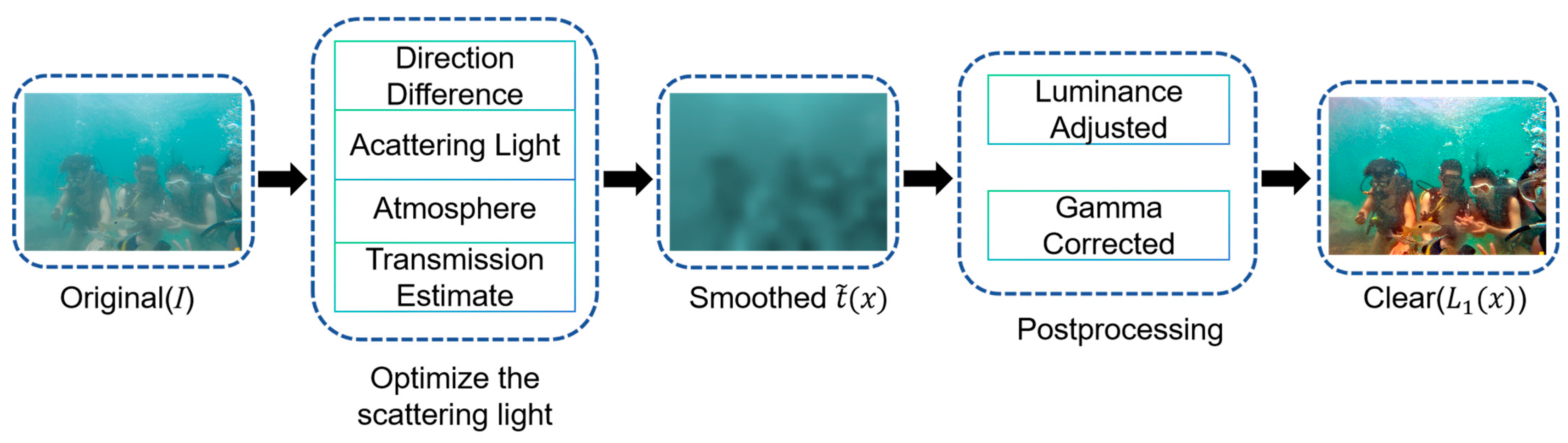
3.4. Visibility Restoration Module

Due to the presence of underwater microorganisms and suspended particles, light is both scattered and absorbed as it propagates through the water. This phenomenon can result in images that are characterized by blurriness and darkness, ultimately leading to reduced visibility. This section addresses this issue by designing an underwater image visibility restoration module that employs an image defogging method based on the rank-one transmission prior [18]. This method assumes that the imaged scene is predominantly illuminated by spatially homogeneous light, except in the vicinity of the light source. The thickness of the scattered light is influenced by the depth of the scene and the degree of light transmission. Based on the theory of underwater optical imaging [23], the influence of the water body on light propagation is primarily manifested through three physical effects: the forward scattering effect caused by suspended particles, the backward scattering effect resulting from the water itself, and the direct attenuation effect that occurs during light transmission. The experimental data indicate that when the shooting distance is less than 2 m, the contribution of the forward scattering component to imaging quality decreases to less than 5%, rendering it negligible.
I c D c + B c
where I c is the image taken directly under water, D c is the direct attenuation component and B c is the backscattering component, Equation (10) can be further subdivided as follows:
I c x = J c x t c x + A c 1 t c x
In Equation (11), x is the coordinate of any pixel in the image. c is the R, G, and B color channels of an image. J c x represents the ideal clear image. A c R 1 × 1 × 3 represents the ambient background light intensity in the R, G, and B channels, t c R m × n × 3 and t c x represent the transmittance of each pixel. The value of this is related to the absorption and scattering of the light waves by seawater in the scene, and the expression is as follows:
t c x = e β λ d x
β(λ) is the attenuation coefficient, including the effect of absorption of the light wave scattering effect. Since the attenuation coefficients of underwater light are different for different frequencies, they vary with the color channel. d x is the scene depth.
The transmittance of the portion of ambient scattered light that affects imaging is described in Equation (11) by 1 t c x , where t ~ is used to denote the transmission map. Transmittance t ~ is strongly correlated with the scattered light, and if the spectrum of the scattered light is given, then the transmittance can be expressed as their correlation coefficient. Assuming that L1 denotes an image of an ideal outdoor scene, image I is the image to be processed of size m × n, and the transmittance map t ~ x R 1 × 3 forms the rank-one prior matrix T ~ R r × 3 r = m × n . t ~ x + t c x = 1,1 , 1 . The relation between the transmittance map t ~ (x) and the spectrum is
t ~ x = C x b
where C R r is the vector of coefficients, b R 1 × 3 is the transport basis of t ~ , and t ~ R m × n × 3 . The modulo expansion of t ~ is the matrix T ~ R 3 × r with the expression:
T ~ = c b
where c is the column main order vector of C . T ~ is the rank-one matrix and the first-order prior on the scattering map.
With the introduction of the rank-one prior, the traditional physical model of optical imaging is defined:
L 1 x = I x ω t ~ x A max 1 ω t ~ x , t 0
t ~ x = I x , S n u S n u
S u c = 1 Ω x Ω I c x , c R , G , B
where A is the ambient light, Ω is the domain of pixel positions with mn elements, ω 0,1 is an introduced constant relaxation parameter and t 0 is the lower bound for the stabilization calculation. Note that t ~ x + t c x = ( 1 , 1 , 1 ) , x Ω . In this section, t 0 is set to 0.001. S n u is the result of normalizing S u c , which can approximate the direction of transmission, and L 1 x is the output image. The physical model performs well in image defogging and deblurring tasks. The reduction in scattered light in underwater images results in clearer images. As shown in Figure 4, it is the processing of the visibility restoration module.

3.5. Comparative Enhancement Module

Underwater image quality is frequently compromised by complex optical environments, which are characterized by non-uniform light distribution, reduced detail contrast, and blurring effects caused by the scattering of suspended particles. The contrast enhancement module improves color saturation and contrast, thereby highlighting the textural details of the image. This enhancement facilitates subsequent analysis and processing.
The AGCWD [24] algorithm dynamically adjusts image luminance through gamma correction while incorporating a weighted probability distribution of pixel intensities, thereby effectively improving the visibility of underexposed regions while maintaining preserving natural image appearance. Assume that X represents I c or Z ^ x and that its luminance l varies in the range of l m i n and l m a x . The dynamic range of the image X(i, j) luminance gray scale I is l m i n and l m a x , where l m i n is the smallest gray scale order. The probability density function of the gray scale pixel distribution of a statistical image:
p d f l = n l M N
where MN is the total number of pixels and nl is the number of pixels corresponding to the gray scale n.
The optimal tuning of the probability density function (pdf) is achieved by utilizing cdf and the normalized gamma transform curve while preserving the statistical properties of the original histogram. Specifically, the probability density function is initially calculated based on the statistical histogram from the previous step. Subsequently, the weighted distribution (WD) function is introduced to correct the histogram, ultimately resulting in the optimized weighted probability density function:
p d f w l = max p d f × p d f l min p d f max p d f min p d f α
A lower gamma parameter produces a more significant adjustment and can take the value [0.1, 0.5], which can be taken as 0.5 as a rule of thumb to give a smoother function curve. We calculate the cumulative distribution function (cdf) using A to carry out the normalization. Using the weighted probability density function calculated from Equation (19), the smoothed cumulative distribution function is derived:
c d f s l = l = l m i n l m a x p d f w f p d f w
T l = l m a x l m i n l l m a x l m i n γ
γ = 1 c d f s l P
T(l) is the transform function. Adaptive gamma correction uses the image cumulative distribution function information cdf of Equation (20), where P denotes the adaptive parameter, set to 1, with a range of values [0.5, 1].
L 2 x = T X i , j
Mapping the luminance values of each pixel point of the image gives the contrast-enhanced image L 2 x .

3.6. Fusion Module

In this section, a multi-scale feature fusion strategy is employed to co-fuse the visibility-restored processed image with the contrast-enhanced image. A multi-exposure image fusion method, which utilizes adaptive weights that reflect relative pixel intensities and global gradients, aims to fully leverage multiple sources of information and construct more effective fusion weights. This method innovatively introduces a dual weighting mechanism that incorporates local weights based on pixel intensities and global gradients. This approach optimally fuses visibility restoration images with contrast enhancement images [25].

3.6.1. Weighted Design Based on Pixel Intensity

The pixel intensity weighting design computes pixel intensity weights derived from pixel intensity values, which are utilized to emphasize the brightness information across images captured with varying exposures.
The pixel intensity-based weighting design regulates the weights to correspond with the overall brightness of the image, considering the presence of more well-exposed pixels when there is a significant difference between the input image and its neighboring exposed images. Consequently, the first weight is denoted as
w 1 , n x = exp L n x 1 m n 2 2 σ n 2
In Equation (24),
σ n = 2 α m n + 1 m n n = 1 α m n + 1 m n 1 1 < n < N 2 α m n m n 1 n = N
N is the number of images in a set of multiple exposure images. L n x is the pixel intensity of the nth image. m n denotes the average of the pixel intensities of the nth image. When L n x is close to 1 m n , the weight is significant, denoted by exp L n x 1 m n 2 . The assignment takes into account the exposure levels of the input image and its neighboring images. σ n varies with different levels of brightness differences. The authors of the original article proposed setting α to 0.75, a value that was also validated by An et al. [26] in underwater images. Consequently, we have also set the value of α to 0.75. w 1 , n x represents the first weight that encodes the relative luminance.

3.6.2. Weighted Design Based on Global Gradient

Traditional methods primarily assign fusion weights based on the local gradient magnitude in multi-exposure image fusion. While this approach effectively preserves the detailed features of high-contrast regions, it may overlook the exposure quality of low-gradient areas. An innovative weight assignment strategy based on cumulative histogram analysis evaluates exposure quality by analyzing the distribution characteristics of pixel intensities. Specifically, the differential properties of the cumulative histogram can reveal pixel distribution patterns under varying exposure conditions. In underexposed images, the cumulative histogram displays a steep upward trend in the low-intensity interval, indicating a significant presence of saturated pixels in this region. Conversely, in moderately exposed images, the cumulative histogram exhibits a more gradual increase, reflecting a more uniform distribution of pixel values. When a pixel is situated in an interval with a lower rate of change in the cumulative histogram, it suggests that the intensity value is statistically rare, thus identifying it as a quality exposure region. Consequently, these observations were encoded as weights:
w 2 , n x = Grad n L n x 1 n = 1 N Grad n L n x 1 + ϵ
To prevent the denominator from becoming zero, a small positive value, denoted as ϵ, is added to it. Grad n · denotes the gradient of the cumulative histogram, which is called the global gradient. In the field of image processing, the global gradient characterizes the gradient features of similar regions across a large area of the image, in contrast to the local gradient, which only reflects variations in the vicinity of a specific pixel. This global analysis method captures the structural features and spatial distribution patterns of an image more comprehensively. During the weight calculation process, local gradient weights must be effectively combined with global gradient weights, and their coordination is achieved through normalization. The final weight calculation formula can be expressed as follows:
W n x = w 1 , n x × w 2 , n x n = 1 N w 1 , n x × w 2 , n x + ϵ
W n x denotes the normalization result of the two weights for each image. Therefore, the final fusion result of the model is shown in Equation (28):
F x = W 1 x L 1 x + W 2 x L 2 x

4. Experiment

We first present the experimental details of the UMMC underwater image enhancement method in the experimental section. Next, we conduct experiments using various datasets to compare our approach with mainstream methods. We perform both quantitative and qualitative analyses based on comparative tests conducted on real and synthetic underwater images. Subsequently, a keypoint matching algorithm is executed [27]. Finally, the operational performance of the proposed method is validated through runtime testing.

4.1. Experimental Details

The primary objective of this section is to compare the proposed underwater image enhancement algorithm with ten widely used underwater image enhancement algorithms. In this experiment, we utilized underwater image datasets, including the UIEB dataset [6], the SUID dataset [28], and the EUVP dataset [29].
The UIEB dataset [6] serves as a benchmark for real underwater imagery and comprises 890 sets of paired data, along with 60 sets of unreferenced challenging samples. This dataset encompasses a wide range of typical underwater imaging conditions, including natural illumination, artificial light sources, and mixed lighting scenarios. The construction process for the reference image synthesizes the outputs of 12 classical enhancement algorithms, selecting the enhancement that best aligns with human visual perception through subjective evaluation. Additionally, the SUID synthetic dataset [28] systematically simulates 900 sets of underwater images, varying in turbidity levels and types of degradation. The EUVP datasets [29] are a large number of high-quality underwater images captured by high-resolution camera equipment and specialized underwater photography.
We randomly selected 100 pairs of images from the UIEB dataset, which included reference images, and 30 pairs of images from the SUID dataset for both quantitative and qualitative evaluations. Additionally, we selected 50 images from the EUVP dataset to conduct runtime duration tests.

4.1.1. Comparative Methods

We compare UMMC with seven UIE methods to validate our superior performance. The methods include an underwater image enhancement method based on an attention mechanism and adversarial autoencoder (UW-AAE) [30], an underwater image enhancement method by correcting color distortion, enhancing contrast, and enriching details (EUICCCLF) [31], a technique focused on minimizing color loss and enhancing local adaptive contrast (MLLE) [32], a method for optimizing contrast enhancement through piecewise color correction and dual prior (PCDE) [33], an underwater image enhancement convolutional neural network model based on underwater scene prior (UWCNN) [34], which we designate as Type I enhancement, an image enhancement technique that separates content and style (UIESS) [35] and a Bayesian Retinex algorithm for enhancing a single underwater image using multi-order gradient priors of reflectance and illumination (BRUIE) [36].

4.1.2. Metrics

For the UIEB dataset, we employed the Natural Image Quality Evaluator (NIQE) [37], the Underwater Color Image Quality Evaluator (UCIQE) [38], and the Non-Reference Underwater Image Quality Measurement (UIQM) [39] assessment metrics. For real underwater images (the UIEB dataset), the selected no-reference quality evaluation metrics are UCIQE and UIQM, both of which exhibit a positive correlation with image quality. In contrast, the NIQE metric shows a negative correlation. Together, these three metrics reflect the degree of consistency between enhancement results and human visual perception. For synthetic underwater images (the SUID dataset), a full-reference evaluation system is employed. In this system, PSNR [40] quantifies the pixel-level similarity between the enhanced image and the reference image, while SSIM [41] assesses the degree of match between the two images in terms of structural features.

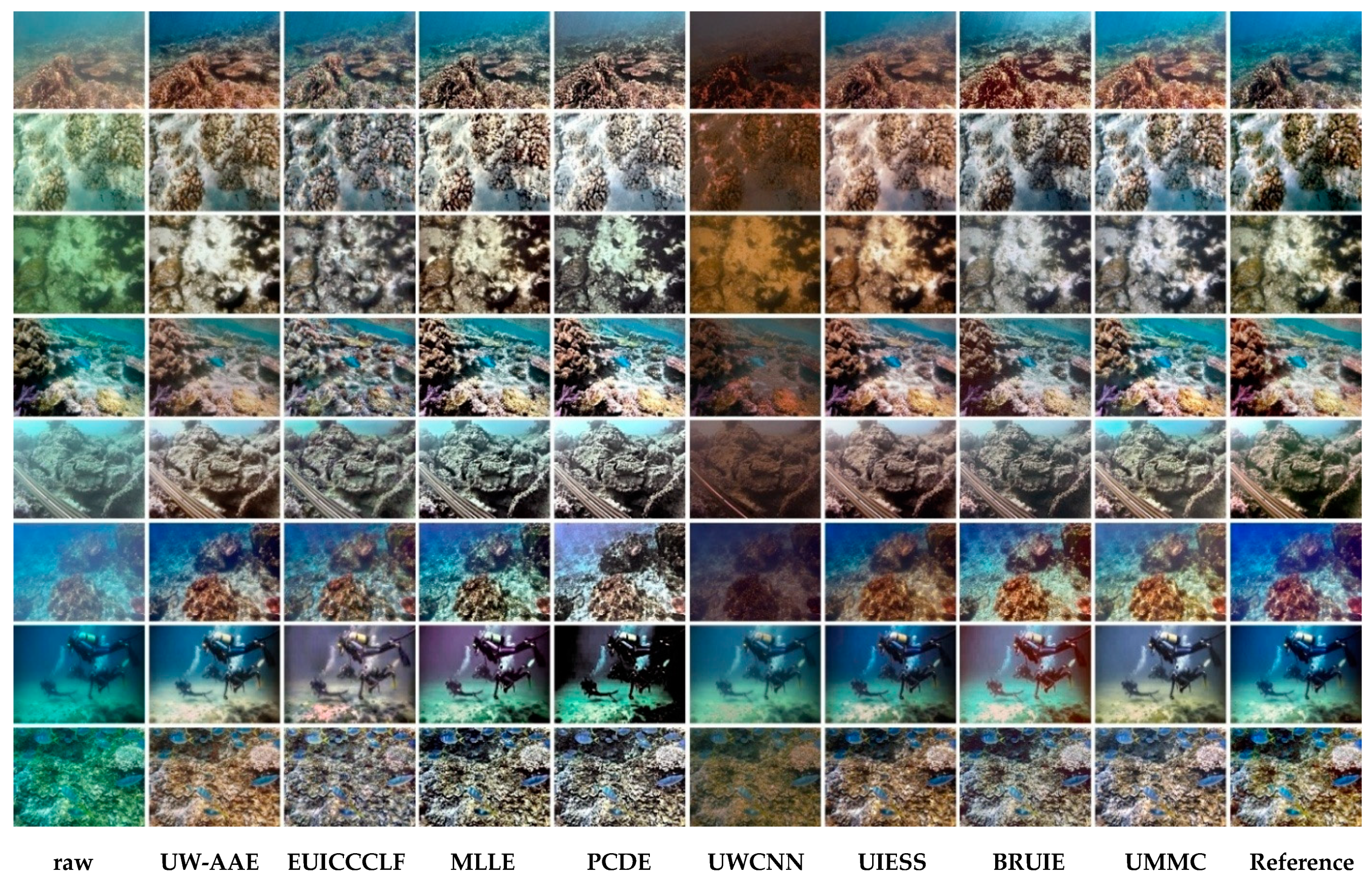
4.2. UIEB Dataset Evaluation

This section is evaluated for a randomly selected set of images from a dataset with reference images. Out of 100 randomly selected pairs of images, underwater images of different underwater scenes are chosen to be presented in the subjectivity assessment to go through the enhancement characteristics of different methods.
The output depicted in Figure 5 demonstrates that the UIESS algorithm obviously improves the image brightness and improves the original color bias but introduces a slight color distortion. The MLLE algorithm successfully resolves the color cast issue and restores the image’s colors effectively, but the brightness is excessively high, resulting in a loss of detail. UW-AEE handles blue-green tinted images well, but it is not as effective in terms of defogging effects and boosting contrast. EUICCCLF has the problem of color loss. With UWCNN, it can be clearly seen that the enhancement is poor. PCDE has the problem of detail loss, and BRUIE has the problem of insufficient color compensation and local darkness. Our algorithm outperforms others in processing images with varying color shades, improving brightness and visibility. However, the saturation enhancement is somewhat excessive and requires further optimization.
Table 1 presents the evaluation results for the real-world dataset. As indicated in the table, our method outperforms all other approaches. This demonstrates that our method effectively compensates for the color absorption in underwater images while preserving more information.

4.3. SUID Dataset Evaluation

In this section, we present and conduct quantitative experiments on 30 randomly selected pairs of images, choosing generated underwater images with different color shifts, turbidity, and low light in comparison to standard images in a subjectivity assessment of the 30 images.
As illustrated in Figure 6, UMMC and MLLE had the best overall performance in terms of visual representation in the SUID dataset. Compared to MLLE, UMMC handles the foggy and turbid images with average results, but the images are more detailed. EUICCCLF shows unwanted color distortion. PCDE makes the images too dark overall. UIESS images show non-yellow tones overall. BRUIE removes the fog better, with noise and localized over-darkness in some of the images. The UW-AAE enhancement is mediocre and does not effectively deal with color casts and only slightly improves them. UWCNN effectively improved the blue-green bias, but new color problems arose and it did not defog well.
Table 2 shows the evaluation of the SUID synthetic dataset, and the results for both data demonstrate the high visual quality of the processing effect of our method. It is also verified that in the subjective assessment, our enhancement results in richer details and a reduction in the loss of structural information compared to other images.

4.4. Keypoint Matching

By applying the keypoint matching algorithm to underwater images, we can extract rich feature point information that significantly enhances target detection and recognition. A higher number of feature points in image matching indicates a greater wealth of information contained within the image, thereby improving the algorithm’s performance.
In this section, an underwater image is randomly selected, and the original image is rotated by 180 degrees to align the feature points with those of the original image. The results of feature point matching using different algorithms are presented in Figure 7. As can be seen from Table 3, the results of the keypoint matching experiment show that the method of this paper does not achieve good results in this experiment, which is in the middle of the range of various methods.

4.5. Ablation Study

We conducted ablation experiments to systematically validate the role of each module in the proposed methodology. We progressively removed or replaced key components of the model using the control variable method, including the following: (a) white balance and visibility restoration only (WBVR), (b) white balance and contrast enhancement only (WBCE), (c) white balance only (WB), (d) contrast enhancement only (CE), (e) visibility restoration only (VR), and (f) the complete method (UMMC). Figure 8 presents a visual comparison of these approaches. The experimental results indicate that CE significantly improves the brightness of the image, while WB effectively reduces color deviation; however, it also contributes to the overall darkening of the image. Both VR and WBVR tend to produce oversaturation, which can lead to a loss of detail. Additionally, under uneven lighting conditions, the visibility of dark details is enhanced, but the lighter areas become overexposed, resulting in color distortion. Black artifacts may appear at the junctions of visible content and darker regions, highlighting a limitation of the visibility restoration module (VR) when applied to non-uniformly illuminated images. WBVR corrects color bias to a certain extent compared to VR, underscoring the importance of WB. After fusing with contrast-enhanced images, UMMC compensates for the deficiencies of VR, further demonstrating the superiority of the UMMC full model. In contrast, WBCE enhances image details without equally compensating for color accuracy. UMMC effectively integrates WBVR and WBCE, resulting in images characterized by uniform colors and rich details. The results in Table 4 demonstrate the effectiveness of UMMC.

4.6. Parameters and FLOPs

In this study, the computational performance of each method was systematically evaluated. The experimental configurations are as follows: the hardware platform consists of an Intel Core i7-13620H processor (4.9 GHz) with 16 GB of RAM. Fifty test images, each measuring 256 × 256 pixels, were randomly selected from the EUVP dataset. All methods were tested on the same computer, which was equipped with an Intel® Core™ i7-13620H CPU operating at 4.9 GHz and 16 GB of RAM. EUICCCLF, MLLE, PCDE, BRUIE, and our method were implemented in MATLAB (R2023b), while the UIESS and UWCNN methods were developed using PyTorch (1.12.0), and the UW-AEE method was implemented in TensorFlow (1.14.0). Table 5 presents a comparison of the average runtimes for the different UIE methods. The experimental results indicate that our method demonstrates superior performance in UIE experiments.

4.7. Summary

Through the above experiments, we found that UMMC achieved good results overall in the six experimental tests. For underwater image enhancement, we successfully eliminated color bias while largely preserving image quality. At the same time, we also found that it is easy to overcompensate when the degree of color bias is small, and for foggy images, it does not work as well as it should, and the processing effect is poor. The modeling algorithm needs to be adjusted in the future. UMMC runs faster while ensuring quality. The significance of each component of UMMC and its overall performance is further illustrated through the ablation experiment. However, the feature point matching test did not achieve the desired results; the model needs to be further adjusted for analysis.

5. Conclusions

In this paper, a multi-module combination of underwater image enhancement algorithm UMMC is proposed to address the problems of the color distortion, low visibility and low brightness of underwater images. Our approach involves the development of a new network designed to improve enhancement performance through five key modules: the color detection module, the color and white balance correction module, the visibility restoration module, the contrast enhancement module, and the image fusion module. After experimental validation, the method proposed in this paper effectively addresses the issues of color cast and low brightness, making it highly suitable for enhancing real underwater images. Furthermore, our model not only improves image quality but also operates with a faster runtime.
Although UMMC has achieved significant results, there are still several limitations that need to be addressed. For the issue of supersaturation in images with low levels of chromatic aberration, as well as in foggy images that are typically processed, it is essential to optimize algorithms and explore new solutions in the future. In addition, the setting of K is also limiting to some extent, and as the next step, we will look for new ways to address this shortcoming such as introducing an adaptive threshold that depends on the image statistics, K. This optimization will be particularly beneficial in addressing a wider range of underwater image challenges. In the future, we plan to adopt a combined approach with deep learning to explore real-time processing and optimization in low-resource environments.

Author Contributions

Z.J.: writing—reviewing and editing, writing—original draft, validation, supervision, software, methodology, survey, funding acquisition, formal analysis, data organization, conceptualization. H.W.: writing—review and editing, writing—original draft, visualization, validation, software, methodology, survey, data curation, conceptualization. G.H.: data organization, investigation, resources, supervision, validation, writing—review and editing. J.C.: data organization, investigation, supervision, visualization. W.F.: conceptualization, funding acquisition, investigation, resources, supervision, writing—review and editing. G.L.: funding acquisition, investigation, resources, supervision—reviewing. All authors have read and agreed to the published version of the manuscript.

Funding

This work was supported by the Shanghai Municipal Industrial Collaborative-Innovation Science and Technology Project [XTCX-KJ-2023-2-15], and the National Key Research and Development Program of China, grant number 2022YFD2401100.

Institutional Review Board Statement

Not applicable.

Informed Consent Statement

Not applicable.

Data Availability Statement

The data presented in this study are available on request from the corresponding author. The data are not publicly available due to copyright issues with co-developers.

Conflicts of Interest

The authors declare no conflict of interest.

References

  1. Luo, G.; Wang, Z.; Chen, Y.; Wang, F.; Zhang, J.; Ma, Z.; Jiang, Z. Design and hydrodynamic analysis of an automated polymer composite mattress deployment system for offshore oil and gas pipeline protection. Mar. Georesour. Geotechnol. 2024, 1–17. [Google Scholar] [CrossRef]
  2. Khan, A.; Ali, S.S.A.; Anwer, A.; Adil, S.H.; Mériaudeau, F. Subsea pipeline corrosion estimation by restoring and enhancing degraded underwater images. IEEE Access 2018, 6, 40585–40601. [Google Scholar] [CrossRef]
  3. Azmi, K.Z.M.; Ghani, A.S.A.; Yusof, Z.M.; Ibrahim, Z. Natural-based underwater image color enhancement through fusion of swarm-intelligence algorithm. Appl. Soft Comput. 2019, 85, 105810. [Google Scholar] [CrossRef]
  4. Desai, C.; Tabib, R.A.; Reddy, S.; Patil, U.; Mudenagudi, U. RUIG: Realistic underwater image generation towards restoration. In Proceedings of the IEEE/CVF Conference on Computer Vision Pattern Recognition Workshops, Virtual, 19–25 June 2021; pp. 2181–2189. [Google Scholar] [CrossRef]
  5. Muhammad, N.; Arini; Fahrianto, F.J. Underwater image enhancement using guided joint bilateral filter. In Proceedings of the 2018 6th International Conference on Cyber and IT Service Management (CITSM), Parapat, Indonesia, 7–9 August 2018; pp. 1–6. [Google Scholar]
  6. Li, C.; Guo, C.; Ren, W.; Cong, R.; Hou, J.; Kwong, S.T.W.; Tao, D. An underwater image enhancement benchmark dataset and beyond. IEEE Trans. Image Process. 2019, 29, 4376–4389. [Google Scholar] [CrossRef]
  7. Ding, W.; Bi, D.; He, L.; Fan, Z. Contrast-enhanced Fusion of Infrared and Visible Images. Opt. Eng. 2018, 57. [Google Scholar] [CrossRef]
  8. Zhang, W.; Dong, L.; Zhang, T.; Xu, W. Enhancing Underwater Image Via Color Correction and Bi-interval Contrast Enhancement. Signal Process. Image Commun. 2021, 90, 116030. [Google Scholar] [CrossRef]
  9. Zhang, W.; Wang, Y.; Li, C. Underwater Image Enhancement by Attenuated Color Channel Correction and Detail Preserved Contrast Enhancement. IEEE J. Ocean. Eng. 2022, 47, 718–735. [Google Scholar] [CrossRef]
  10. Xu, H.; Ma, J.; Jiang, J.; Guo, X.; Ling, H. U2Fusion: A Unified Unsupervised Image Fusion Network. IEEE Trans. Pattern Anal. Mach. Intell. 2020, 44, 502–518. [Google Scholar] [CrossRef]
  11. Zhang, H.; Xu, H.; Xiao, Y.; Guo, X.; Ma, J. Rethinking the Image Fusion: A Fast Unified Image Fusion Network Based on Proportional Maintenance of Gradient and Intensity. Proc. AAAI Conf. Artif. Intell. 2020, 34, 12797–12804. [Google Scholar] [CrossRef]
  12. Tang, L.; Yuan, J.; Ma, J. Image Fusion in the Loop of High-Level Vision Tasks: A Semantic-Aware Real-Time Infrared and Visible Image Fusion Network. Inf. Fusion 2022, 82, 28–42. [Google Scholar] [CrossRef]
  13. Arya, P.; Kumar, S.; Agarwal, A.; Yenneti, N.; Pai, N. Redefining Well Exposedness for Locally Adaptive Multi-Exposure Fusion. In Proceedings of the ICASSP 2025–2025 IEEE International Conference on Acoustics, Speech and Signal Processing (ICASSP), Hyderabad, India, 6–11 April 2025; pp. 1–5. [Google Scholar] [CrossRef]
  14. Sudhanthira, K.; Sathya, P.D. Color Balance and Fusion for Underwater Image Enhancement. Pramana Res. J. 2019, 9, 1–13. [Google Scholar]
  15. Jiang, Q.; Zhang, Y.; Bao, F.; Zhao, X.; Zhang, C.; Liu, P. Two-step Domain Adaptation for Underwater Image Enhancement. Pattern Recognit. 2022, 122, 108324. [Google Scholar] [CrossRef]
  16. Zhou, J.; Sun, J.; Zhang, W.; Lin, Z. Multi-view Underwater Image Enhancement Method Via Embedded Fusion Mechanism. Eng. Appl. Artif. Intell. 2023, 121, 105946. [Google Scholar] [CrossRef]
  17. Zhang, W.; Zhou, L.; Zhuang, P.; Li, G.; Pan, X.; Zhao, W.; Li, C. Underwater Image Enhancement Via Weighted Wavelet Visual Perception Fusion. IEEE Trans. Circuits Syst. Video Technol. 2024, 34, 2469–2483. [Google Scholar] [CrossRef]
  18. Liu, J.; Liu, R.W.; Sun, J.; Zeng, T. Rank-one prior: Real-time scene recovery. IEEE Trans. Pattern Anal. Mach. Intell. 2022, 45, 8845–8860. [Google Scholar] [CrossRef] [PubMed]
  19. Li, F.; Wu, J.; Wang, Y.; Zhao, Y.; Zhang, X. A color cast detection algorithm of robust performance. In Proceedings of the IEEE Fifth International Conference on Advanced Computational Intelligence, Nanjing, China, 18–20 October 2012; pp. 662–664. [Google Scholar]
  20. Gasparini, F.; Schettini, R. Color correction for digital photographs. In Proceedings of the 12th International Conference on Image Analysis and Processing, Mantova, Italy, 17–19 September 2003; pp. 646–651. [Google Scholar] [CrossRef]
  21. Wang, Y.; Tang, C.; Cai, M.; Yin, J.; Wang, S.; Cheng, L.; Wang, R.; Tan, M. Real-time underwater onboard vision sensing system for robotic gripping. IEEE Trans. Instrum. 2021, 70, 1–11. [Google Scholar] [CrossRef]
  22. Afifi, M.; Brown, M.S. Interactive White Balancing for Camera-Rendered Images. Color Imaging Conf. 2020, 28, 136–141. [Google Scholar] [CrossRef]
  23. Jaffe, J. Computer modeling and the design of optimal underwater imaging systems. IEEE J. Ocean. Eng. 1990, 15, 101–111. [Google Scholar] [CrossRef]
  24. Huang, S.-C.; Cheng, F.-C.; Chiu, Y.-S. Efficient contrast enhancement using adaptive gamma correction with weighting distribution. IEEE Trans. Image Process. 2012, 22, 1032–1041. [Google Scholar] [CrossRef]
  25. Lee, S.-H.; Park, J.S.; Cho, N.I. A multi-exposure image fusion based on the adaptive weights reflecting the relative pixel intensity and global gradient. In Proceedings of the 2018 25th IEEE International Conference on Image Processing (ICIP), Athens, Greece, 7–10 October 2018; pp. 1737–1741. [Google Scholar]
  26. An, S.; Xu, L.; Deng, Z.; Zhang, H. HFM: A Hybrid Fusion Method for Underwater Image Enhancement. Eng. Appl. Artif. Intell. 2024, 127. [Google Scholar] [CrossRef]
  27. Lowe, D.G. Distinctive image features from scale-invariant keypoints. Int. J. Comput. Vis. 2004, 60, 91–110. [Google Scholar] [CrossRef]
  28. Hou, G.; Zhao, X.; Pan, Z.; Yang, H.; Tan, L.; Li, J. Benchmarking underwater image enhancement and restoration, and beyond. IEEE Access 2020, 8, 122078–122091. [Google Scholar] [CrossRef]
  29. Islam, M.J.; Xia, Y.; Sattar, J. Fast underwater image enhancement for improved visual perceptionn. IEEE Robot. Autom. Lett. 2019, 5, 3227–3234. [Google Scholar] [CrossRef]
  30. Luo, G.; He, G.; Jiang, Z.; Luo, C. Attention-based mechanism and adversarial autoencoder for underwater image enhancement. Appl. Sci. 2023, 13, 9956. [Google Scholar] [CrossRef]
  31. Hu, H.; Xu, S.; Zhao, Y.; Chen, H.; Yang, S.; Liu, H.; Zhai, J.; Li, X. Enhancing Underwater Image via Color-Cast Correction and Luminance Fusion. IEEE J. Ocean. Eng. 2024, 49, 15–29. [Google Scholar] [CrossRef]
  32. Zhang, W.; Zhuang, P.; Sun, H.; Li, G.; Kwong, S.; Li, C. Underwater image enhancement via minimal color loss and locally adaptive contrast enhancement. IEEE Trans. Image Process. 2022, 31, 3997–4010. [Google Scholar] [CrossRef]
  33. Zhang, W.; Jin, S.; Zhuang, P.; Liang, Z.; Li, C. Underwater Image Enhancement via Piecewise Color Correction and Dual Prior Optimized Contrast Enhancement. IEEE Signal Process. Lett. 2023, 30, 229–233. [Google Scholar] [CrossRef]
  34. Li, C.; Anwar, S.; Porikli, F. Underwater scene prior inspired deep underwater image and video enhancement. Pattern Recognit. 2020, 98, 107038. [Google Scholar] [CrossRef]
  35. Chen, Y.-W.; Pei, S.-C. Domain adaptation for underwater image enhancement via content and style separation. ISSS J. Micro Smart Syst. 2022, 10, 90523–90534. [Google Scholar] [CrossRef]
  36. Zhuang, P.; Li, C.; Wu, J. Bayesian retinex underwater image enhancement. Eng. Appl. Artif. Intell. 2021, 101, 104171. [Google Scholar] [CrossRef]
  37. Mittal, A.; Soundararajan, R.; Bovik, A.C. Making a “completely blind” image quality analyzer. IEEE Signal Process. Lett. 2013, 20, 209–212. [Google Scholar] [CrossRef]
  38. Yang, M.; Sowmya, A. An underwater color image quality evaluation metric. IEEE Trans. Image Process. 2015, 24, 6062–6071. [Google Scholar] [CrossRef] [PubMed]
  39. Panetta, K.; Gao, C.; Agaian, S. Human-visual-system-inspired underwater image quality measures. IEEE J. Ocean. Eng. 2016, 41, 541–551. [Google Scholar] [CrossRef]
  40. Korhonen, J.; You, J. Peak signal-to-noise ratio revisited: Is simple beautiful? In Proceedings of the Fourth International Workshop on Quality of Multimedia Experience, Melbourne, VIC, Australia, 5–7 July 2012; pp. 37–38. [Google Scholar]
  41. Horé, A.; Ziou, D. Image quality metrics: PSNR vs. SSIM. In Proceedings of the 20th International Conference on Pattern Recognition, Istanbul, Turkey, 23–26 August 2010; pp. 2366–2369. [Google Scholar]
Figure 1. UMMC results for real and simulated underwater images.
Applsci 15 05200 g001
Figure 2. An overall flowchart of the UMMC algorithm. The input image I(x) undergoes color deviation detection (the K value of the example image used in the flowchart exceeds the predetermined threshold) and subsequently enters the correction process. The corrected image Z ^ (x) undergoes visibility restoration and comparison enhancement to obtain L 1 ( x ) and L 2 x , respectively. Finally, the final resulting image F(x) is obtained after fusion processing.
Applsci 15 05200 g002
Figure 3. Color deviation detection result of underwater image.
Applsci 15 05200 g003
Figure 4. A flowchart of the rank-one prior method.
Applsci 15 05200 g004
Figure 5. A subjective comparison of the UIEB dataset. From left to right are the input image, as well as UW-AEE, EUICCCLF, MLLE, PCDE, UWCNN, UIESS, BRUIE, the proposed UMMC and the reference image.
Applsci 15 05200 g005
Figure 6. Subjective comparison of the SUID dataset. From left to right are the input image, as well as UW-AEE, EUICCCLF, MLLE, PCDE, UWCNN, UIESS, BRUIE, the proposed UMMC and the ground truth image.
Applsci 15 05200 g006
Figure 7. Comparisons of keypoint matching.
Applsci 15 05200 g007
Figure 8. Ablation results for each key component of our method.
Applsci 15 05200 g008
Table 1. An objective assessment of real underwater benchmarks with different algorithms. The best result is in red, whereas the second-best result is in green.
MethodsMetric
NIQEUCIQEUIQM
UW-AAE15.7050.789115.897
EUICCCLF15.4060.704116.363
MLLE12.7712.475114.243
PCDE14.0851.453126.915
UWCNN15.3280.89769.118
UIESS16.8961.05999.772
BRUIE12.9700.812115.0823
UMMC12.6122.532124.220
Table 2. An objective assessment of synthetic underwater images with different algorithms. The best result is in red, whereas the second-best result is in green.
MethodsMetric
PSNRSSIM
UW-AAE9.6790.361
EUICCCLF16.1250.786
MLLE18.0100.752
PCDE14.7030.636
UWCNN16.1620.792
UIESS16.0710.866
BRUIE17.4220.758
UMMC18.2580.824
Table 3. The image feature point matching results for each algorithm are presented. The best result is in red, whereas the second-best result is in green.
MethodsLeft Match PointRight Match Point
Raw11101128
UW-AAE23672341
EUICCCLF41494216
MLLE31323104
PCDE40314054
UWCNN258233
UIESS16371599
BRUIE42604260
UMMC35623474
Table 4. An underwater image quality evaluation of different variants of the presented method. The best result is in red, whereas the second-best result is in green.
MethodsMetric
NIQEUCIQEUIQM
WBVR15.2540.782104.244
WBCE14.3320.633104.375
WB16.4170.703100.291
CE12.9791.757113.581
VR12.7780.784104.663
UMMC12.6122.532124.220
Table 5. Comparison of parameters, FLOPs and runtime on different UIE methods. The best result is in red, whereas the second-best result is in green.
MethodsPlatform#Param.FLOPsTime (s)PSNRSSIM
UW-AAETensorFlow148.77 M2805.34 G6.9717.120.85
EUICCCLFMATLAB--0.0216.820.71
MLLEMATLAB--0.0816.260.64
PCDEMATLAB--0.1615.130.60
UWCNNPyTorch0.04 M2.61 G0.1211.080.30
UIESSPyTorch4.2 M26.35 G0.4323.370.73
BRUIEMATLAB--0.1515.130.60
UMMCMATLAB--0.0718.030.87
Disclaimer/Publisher’s Note: The statements, opinions and data contained in all publications are solely those of the individual author(s) and contributor(s) and not of MDPI and/or the editor(s). MDPI and/or the editor(s) disclaim responsibility for any injury to people or property resulting from any ideas, methods, instructions or products referred to in the content.

