An Improved Multi-Objective Grey Wolf Optimizer for Aerodynamic Optimization of Axial Cooling Fans

Abstract

This paper introduces an improved multi-objective grey wolf optimizer (IMOGWO) and demonstrates its application to the aerodynamic optimization of an axial cooling fan. Building upon the traditional multi-objective grey wolf optimizer (MOGWO), several improvement strategies were adopted to enhance its performance. Firstly, the IMOGWO started population initialization based on the Bloch coordinates of qubits to ensure a high-quality initial population. Additionally, it employed a nonlinear convergence factor to facilitate global exploration and integrated the inspiration of Manta Ray Foraging to enhance the information exchange between populations. Finally, associative learning was leveraged for archive updating, allowing for perturbative mutation of solutions in crowded regions of the archive to increase solution diversity and improve the algorithm’s search capability. The proposed IMOGWO was applied to five multi-objective benchmark functions, comprising three two-objective and two three-objective problems, and experimental results were compared with three well-known multi-objective algorithms: the non-dominated sorting genetic algorithm II (NSGA II), MOGWO, and the multi-objective multi-verse optimizer (MOMVO). It is demonstrated that the proposed algorithm had advantages in convergence accuracy and diversity of solutions, which were quantified by the performance metrics (generational distance (GD), inverted generational distance (IGD), Spacing (SP), and Hypervolume (HV)). Furthermore, a multi-objective optimization process coupled with the IMOGWO algorithm and Computational Fluid Dynamics (CFD) was proposed. By optimizing the design parameters of an axial cooling fan, a set of non-dominated solutions was obtained within limited iteration steps. Consequently, the IMOGWO also presented an effective and practical approach for addressing multi-objective optimization challenges with respect to engineering problems.

1. Introduction

Real-world optimization problems are pervasive across all scientific disciplines and engineering applications, often being naturally formulated as optimization problems. These challenges are characterized by their complexity, including nonlinearity, multiple conflicting objectives, discontinuities, high dimensionality, uncertainties, non-convex regions, etc. The primary aim of multi-objective optimization algorithms is to accurately approximate the true Pareto-optimal solutions while maintaining maximal diversity among these solutions [1]. This diversity is crucial as it provides decision-makers with a comprehensive set of design options. Unlike traditional methods that combine multiple objectives into a single aggregate objective, contemporary multi-objective optimization techniques preserve the distinct multi-objective formulation. This approach allows for the thorough exploration of trade-offs between conflicting objectives, enabling the approximation of the entire Pareto-optimal front within a single optimization process.

Nature-inspired algorithms are widely used for multi-objective optimization problems, and they can be broadly categorized into three types: (1) evolutionary algorithms, (2) swarm intelligence algorithms, and (3) physics-based algorithms [2]. Evolutionary algorithms simulate natural evolutionary processes through iterative optimization, where the best individuals are combined to form new generations. This iterative combination promotes population improvement over successive iterations. Among the most prominent evolutionary algorithms are the non-dominated sorting genetic algorithm II (NSGA II) [3], NSGA III [4,5], and the multi-objective differential evolution algorithm (MODEA) [6].

NSGA II, a well-known evolutionary algorithm for multi-objective optimization, addresses the limitations of its predecessor, NSGA, by incorporating fast non-dominated sorting, an elitist mechanism, and a diversity-preserving operator. It begins with a randomly generated population, classifies individuals into different fronts based on dominance, and determines fitness using front rank and crowding distance. This ensures a diverse set of solutions. Through binary tournament selection, crossover, and mutation, offspring are generated and combined with the parent population. The combined population undergoes non-dominated sorting again, and the best individuals are selected to form the new population. A key feature of NSGA II is its ability to maintain a diverse set of Pareto-optimal solutions via the crowding distance mechanism, which favors individuals in less crowded regions, ensuring a well-distributed Pareto front. This iterative process continues until a termination criterion, typically a maximum number of generations, is met. NSGA II is renowned for its effectiveness in approximating the true Pareto front and maintaining solution diversity, making it a benchmark in multi-objective optimization. Building upon NSGA II, NSGA III introduces enhancements in diversity preservation and efficiency, enabling a more accurate approximation of the Pareto front [4]. However, its performance in high-dimensional objective spaces is somewhat limited in maintaining diversity. The multi-objective differential evolution algorithm (MODEA) modifies the selection scheme of traditional differential evolution to address multi-objective problems, adjusting domination criteria and improving offspring generation before performing domination checks. Despite these improvements, the practical application of differential evolution algorithms for multi-objective optimization, particularly in nutrition decision problems, still requires further enhancement [6].

Physics-based algorithms mimic the fundamental physical laws observed in nature, allowing individuals to communicate and navigate the search space using concepts such as gravitational force, inertia, light refraction, and molecular dynamics. Prominent algorithms in this category include the multi-objective gravitational search algorithm (MOGSA) [7], multi-objective atom search optimizer (MOASO) [8], multi-objective ray optimization algorithm (MOROA) [9], and multi-objective multi-verse optimizer (MOMVO) [10]. MOGSA is inspired by one of nature’s most fundamental forces: gravity. It combines Pareto optimality principles with operators derived from evolutionary algorithms. While gravitational-based algorithms are known for their efficiency, MOGSA tends to have a slightly higher execution time per iteration compared to conventional methods like particle swarm optimization [7]. MOASO leverages molecular forces to provide enhanced capabilities for tackling complex global optimization problems. MOROA employs Snell’s law of refraction to find global solutions by altering the path of light as it travels through materials with different refractive indices. MOMVO adapts the concepts of the multi-verse optimizer to address multi-objective optimization problems. It integrates an archive mechanism to maintain non-dominated solutions and utilizes a leader selection strategy to guide the optimization process. The algorithm initializes a population of solutions evaluated across multiple objectives and employs Pareto dominance principles to classify solutions and update the archive with the best non-dominated solutions. During optimization, MOMVO dynamically adjusts solution positions by exchanging variables between population solutions and those in the archive, balancing exploration and exploitation of the search space. The algorithm’s robustness and ability to maintain solution diversity are enhanced by using multiple operators to induce abrupt changes in solution variables. This makes MOMVO particularly effective for problems with up to three objectives, delivering competitive results in terms of both accuracy and execution time [10].

Swarm intelligence (SI) algorithms are renowned for their decentralized nature, shape-formation capabilities, and self-organization properties. These algorithms are inspired by the collective behaviors of social creatures such as bird flocking, animal herding, and ant foraging. Some of the most popular SI algorithms include the multi-objective particle swarm optimizer (MOPSO) [11], multi-objective cat swarm optimizer (MOCSO) [12], and multi-objective grey wolf optimizer (MOGWO) [13]. MOPSO extends the traditional particle swarm optimization algorithm to handle multi-objective optimization problems. It is a population-based algorithm with relatively simple implementation, incorporating an external archive (referred to as a “repository”) and a geographically inspired strategy to preserve solution diversity [11]. MOCSO, proposed by Pradhan and Panda [12], extends the cat swarm optimization algorithm to multi-objective problems. By incorporating both an external archive and the Pareto dominance criterion, it ensures effective preservation and management of non-dominated solutions. MOGWO is a sophisticated algorithm designed specifically for multi-objective optimization by extending the grey wolf optimizer (GWO) [14,15,16,17]. MOGWO incorporates two key components to enhance its functionality: an archive for storing non-dominated solutions and a leader selection mechanism. The archive preserves the best solutions found during the optimization process, balancing diversity and convergence. The leader selection mechanism involves choosing three leaders ($\alpha$, $\beta$, and $\delta$ wolves) from the archive to guide the search agents. This strategy improves the navigation of the search space by effectively balancing the exploration and exploitation phases, resulting in a well-distributed Pareto front. The algorithm’s effectiveness is due to its unique mechanisms for maintaining diversity and guiding the search process with the best non-dominated solutions. Despite its advantages, MOGWO is particularly suited for problems with up to four objectives and continuous variables, as it faces challenges with a larger number of objectives and discrete variables [13].

Several variants of MOGWO have introduced modifications to specific parameters or operational mechanisms. These modifications are typically incremental in nature and do not constitute fundamental alterations to the underlying structure of the original algorithm. Rather, they are intended to enhance the algorithm’s capability to achieve a more effective balance between exploration and exploitation, particularly in various application scenarios. The binary variant of MOGWO, introduced by Al-Tashi et al. [18], was designed for optimal feature selection and relies on a sigmoid transfer function for binary mapping. Lu et al. [19] introduced a modified version of MOGWO for solving discrete optimization problems. This variant incorporates two discrete individual updating strategies: one based on crossover operations in the tracing mode and another utilizing a memory pool mechanism. In addition, neighborhood structures in the seeking mode were presented to make the algorithm suitable for the multi-objective discrete scheduling problem. Sreenu and Malempati [20] proposed a fractional MOGWO. The functional approach is another adjustment that can influence the performance of MOGWO. The technique is mainly used to guide the wolves’ movement in the search space, and the updating strategy is refined by combining the alpha and beta solutions to improve exploration and exploitation. Sreenu and Malempati [21] proposed another fractional MOGWO approach, which aims to optimize the movement strategy of wolves during the search process and facilitate the generation of higher-quality solutions. There are also several modified versions of MOGWO that have been developed to achieve better global optima and efficiently optimize objectives across various research fields. Yang et al. [22] introduced an enhanced MOGWO by implementing a nonlinear control parameter adjustment strategy to boost exploration capabilities and an advanced search strategy to improve leader exploration. Liu et al. [23] proposed a novel MOGWO variant incorporating various search approaches to address different multi-objective problems. This technique dynamically adjusts the convergence pace and balances exploitation and exploration through an adaptive chaotic mutation method and generational distance adjustments to the archive. Additionally, it integrates crowding distance-based elitism and non-dominated sorting techniques to explore a broader range of Pareto-optimal solutions while maintaining diversity in the solution set. Javidsharifi et al. [24] developed a distance-based strategy to control repository size, ensuring rapid and precise convergence and a well-distributed Pareto front, thereby enhancing the performance of MOGWO search agents. Eappen and Shankar [25] proposed a modified MOGWO to achieve better global optima by maintaining a balance between exploitation and exploration processes. Their modifications included adjustments to discrimination weight, leader selection, and mutation coefficients. To overcome the issues of unreasonable head wolf selection and slow convergence in multi-objective optimization, Zhang et al. [26] proposed an improved multi-objective grey wolf optimizer (IMOGWO), which integrates a reference vector-based head wolf selection mechanism and Levy flight operator to enhance diversity and convergence performance. In addition, to enhance the convergence performance and reduce the risk of local optima in multi-objective grey wolf optimization, Liu et al. [27] presented a Modified Boltzmann-Based MOGWO (MBB-MOGWO), a modified variant incorporating Boltzmann-based selection, which demonstrates superior efficiency on benchmark test functions and real-world IoT service composition tasks.

Despite these improvements, most existing MOGWO variants focus on structural or parameter-level adjustments, lacking a deeper theoretical redesign based on quantum computation principles. Moreover, few approaches explicitly exploit the Bloch coordinates of qubits to enhance exploration–exploitation dynamics in GWO-based multi-objective search. To address this gap, this study introduces an improved multi-objective grey wolf optimizer (IMOGWO) and evaluates its performance using benchmark functions and a real engineering application. The IMOGWO utilizes the Bloch coordinates of qubits to ensure a high-quality initial population. By integrating the concepts of Manta Ray Foraging and associative learning, information exchange between populations and the search capability of the IMOGWO are enhanced. These innovative strategies are incorporated into the original GWO algorithm to achieve better convergence and a more diverse set of high-quality solutions for multi-objective optimization. Detailed improvements are presented in Section 2. In Section 3.1, the practical effects of the IMOGWO are demonstrated through experimental validation using five benchmark functions. The results are compared with three well-known multi-objective algorithms: NSGA II, MOGWO, and MOMVO, showcasing the IMOGWO’s superior coverage and convergence. In Section 3.2, the IMOGWO is applied to a multi-objective process to optimize the aerodynamic performance of an axial cooling fan. Finally, the main conclusions are drawn in Section 4.

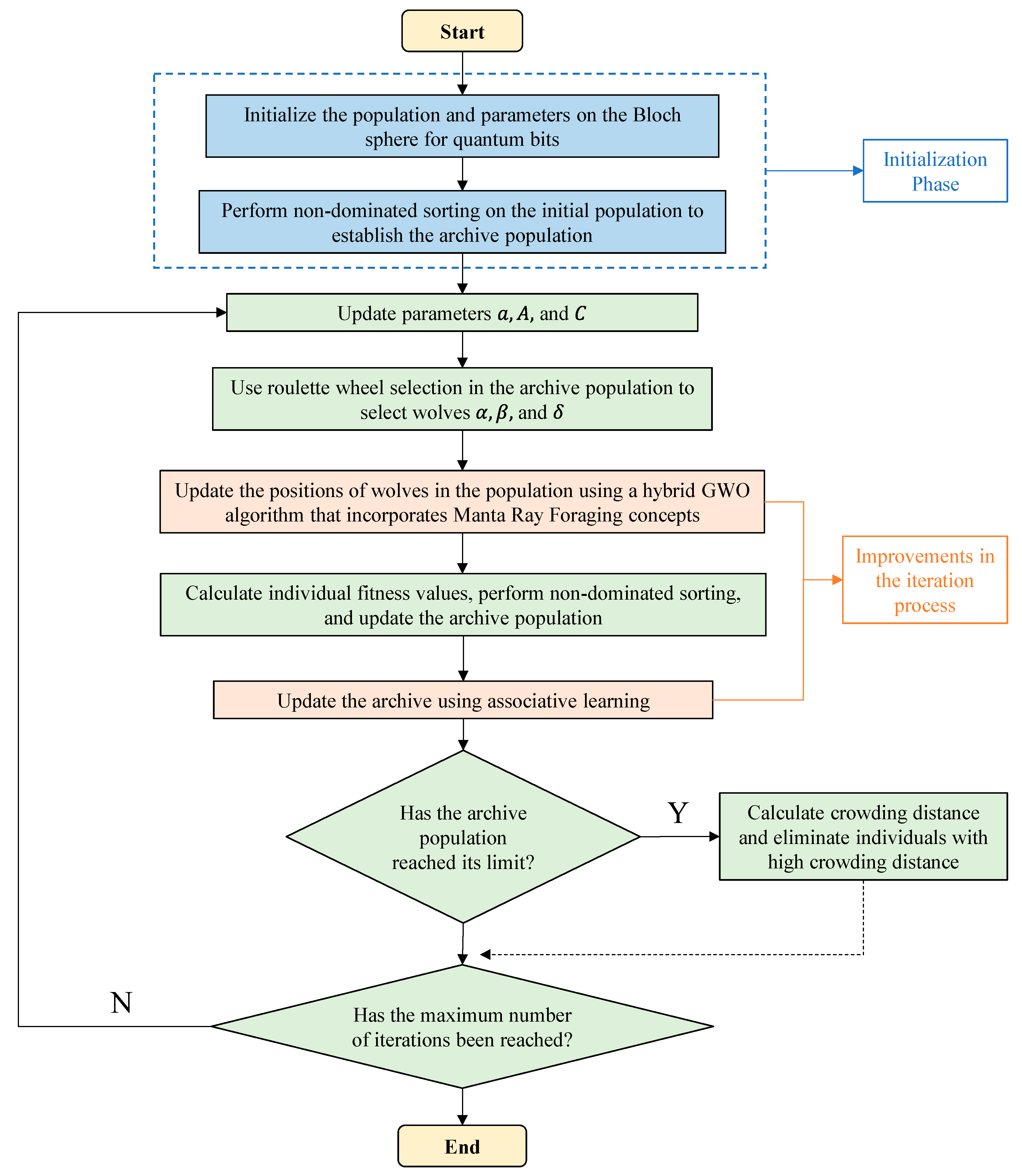
2. Improved Multi-Objective Grey Wolf Optimizer

In order to address optimization problems with multiple objectives, Mirjalili et al. [13] proposed the MOGWO. However, this algorithm has some drawbacks. Firstly, while the original MOGWO improves search performance by selecting the leading wolf from the archive, it struggles to escape local optima if the archive population falls into one. Secondly, the random generation of the initial population can lead to an uneven population distribution and reduce the population diversity. Additionally, although the GWO has a relatively fast convergence speed, its convergence accuracy has room for improvement. Based on these insights, this paper proposes the following improvements to the MOGWO algorithm.

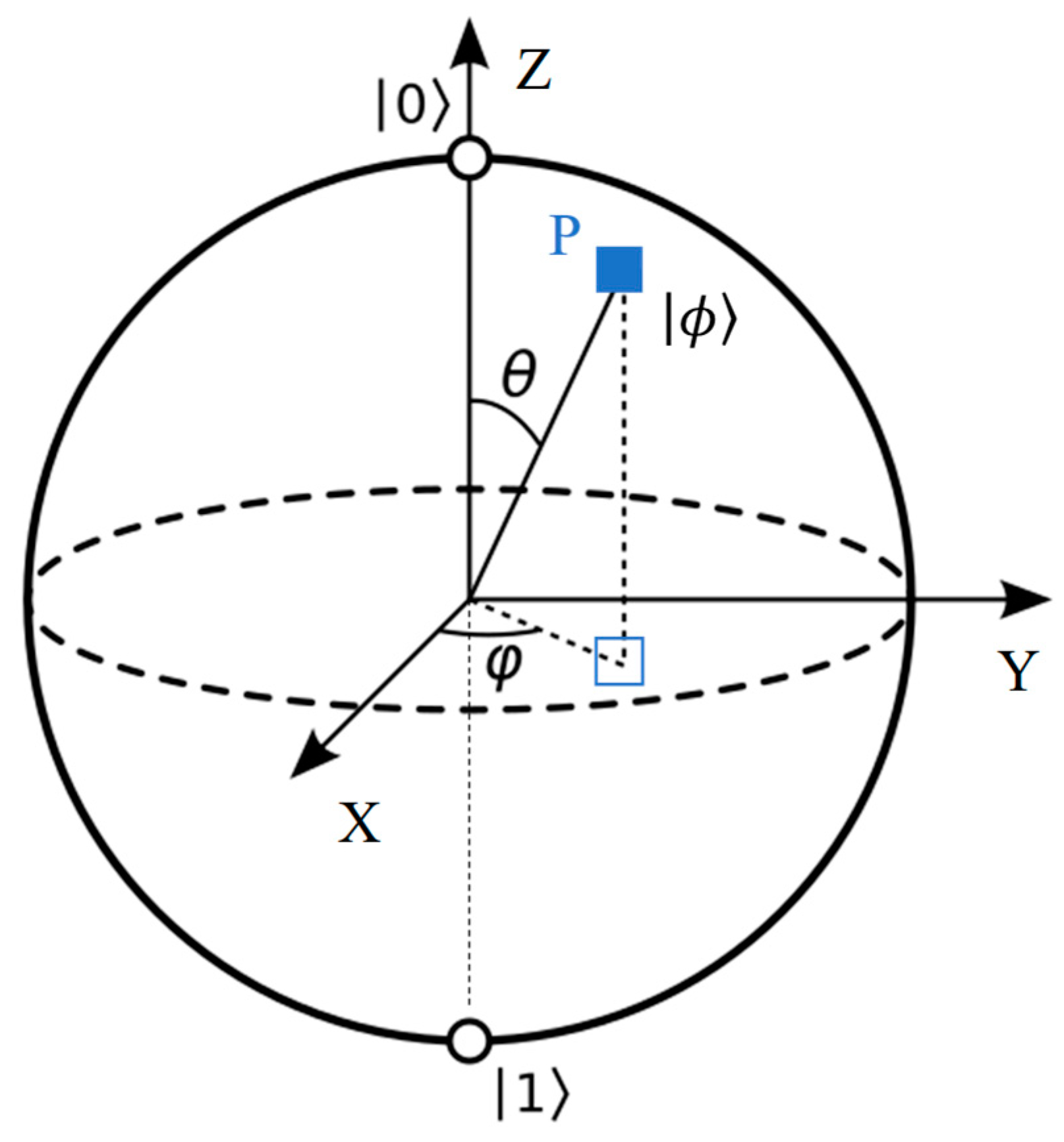
2.1. Population Initialization Based on Bloch Coordinates of Qubits

High-quality initial populations significantly contribute to the convergence speed and solution quality of algorithms. However, the MOGWO algorithm, which employs random initialization of the population, often results in uneven population distribution. This uneven distribution can lead to reduced population diversity and adversely affect the algorithm’s convergence speed. Therefore, this paper adopts the population initialization method based on Bloch coordinates of qubits. The primary principle is introduced below. In quantum computing, the smallest unit of information is the qubit. The state of a qubit can be expressed as follows [28]:

$$\left|\varphi \right.⟩=\cos \left({\displaystyle \frac{\theta }{2}}\right) \left|0\right.⟩+e^{i\phi }\sin \left({\displaystyle \frac{\theta }{2}}\right) |1⟩$$

(1)

where the two parameters on the right side of the equation uniquely determine a point P on the Bloch sphere. Because each point of Bloch spheres $(\theta , \phi )$ corresponds uniquely to a normalized quantum state in terms of $\left|\varphi \right.⟩$. The symbols $\left|0\right.⟩$ and $\left|1\right.⟩$ are the standard basis vectors of quantum states in quantum mechanics, which form the standard orthogonal basis of a two-dimensional Hilbert space, as shown in Figure 1. Since any qubit corresponds to a point on the Bloch sphere, and the Bloch sphere is a three-dimensional unit sphere, the spherical coordinates of a qubit ($|\varphi ⟩$) can also be expressed as follows:

$$|\varphi ⟩={[cos\phi sin\theta sin\phi sin\theta cos\theta ]}^T$$

(2)

Thus, grey wolf individuals can be encoded using the Bloch spherical coordinates of qubits. Let $P_i$ be the $i$-th individual in the population, and n be the optimization dimension; then its encoding strategy is described as follows:

$$P_i=\left[\begin{array}{c}cos{\phi }_{i1}sin{\theta }_{i1}\\ sin{\phi }_{i1}sin{\theta }_{i1}\\ cos{\theta }_{i1}\end{array}\right]\dots \left[\begin{array}{c}cos{\phi }_{in}sin{\theta }_{in}\\ sin{\phi }_{in}sin{\theta }_{in}\\ cos{\theta }_{in}\end{array}\right]$$

(3)

The parameters (${\phi }_{ij}$ and ${\theta }_{ij}$) are random numbers in the range [0, 2π] and [0, π], respectively, and $i=1,2,\dots ,m,j=1,2,\dots n$, where $m$ represents colony size, and $n$ represents the number of qubits. The Bloch coordinates of each qubit can be regarded as three paratactic gene chains, each of them representing a solution; thus, an individual can simultaneously represent three solutions:

$$\left\{\begin{array}{c}{P}_{i,x}=[cos{\phi }_{i1}sin{\theta }_{i1}\dots cos{\phi }_{in}sin{\theta }_{in}]\\ P_{i,y}=[sin{\phi }_{i1}sin{\theta }_{i1},\dots ,sin{\phi }_{in}sin{\theta }_{in}]\\ P_{i,z}=[cos{\theta }_{i1},cos{\theta }_{i2},\dots ,cos{\theta }_{in}]\end{array}\right.$$

(4)

where $P_{i,x}$ is known as the x solution, $P_{i,y}$ is known as the y solution, and $P_{i,z}$ is known as the z solution. The individual encoded by the qubits is shown in Figure 2.

Each individual contains 3$n$ Bloch coordinates of $n$ qubits that can be transformed from the unit space ${[-1,1]}^n$ to the solution space of the continuous optimization problem. It is assumed that $(x_{ij},y_{ij},z_{ij})$ denote the Bloch coordinates of the $j$-th qubit in the $i$-th individual. The corresponding variables $(X_{i,x}^j,X_{i,x}^j,X_{i,x}^j)$ in the solution space are, respectively, computed as follows:

$$\left\{\begin{array}{c}{X}_{i,x}^j=0.5[{ub}_j\left(1+x_{ij}\right)+{lb}_j\left(1-x_{ij}\right)]\\ X_{i,y}^j=0.5[{ub}_j\left(1+y_{ij}\right)+{lb}_j\left(1-y_{ij}\right)]\\ X_{i,z}^j=0.5[{ub}_j\left(1+z_{ij}\right)+{lb}_j\left(1-z_{ij}\right)]\end{array}\right.$$

(5)

where [${lb}_j$, ${ub}_j$] are the lower and upper bounds of the corresponding variables. Thus, three feasible solutions are obtained, and the best fitness among them is used as the encoding of the individual. That improves the quality of the initial population distribution in the search space and enhances the global search capability. The pseudo-code for population initialization based on the Bloch coordinates of qubits is presented in

Table 1. The pseudo-code of the Bloch qubit spherical initialization population.

For each individual$i$ in the population size (Popsize):

Set Grey Wolves[$i$].Velocity to 0 Initialize Grey Wolves[$i$].Position as a zero vector of length $n$Var % The three coordinates of qubits For each variable $j$ in $n$Var: Generate random angle $\phi$ in the range [0, 2$\pi$] Generate random angle $\theta$ in the range [0, 2$\pi$] Calculate chrom1[$j$] as cos($\phi$) sin($\theta$) Calculate chrom2[$j$] as sin($\phi$) sin($\theta$) Calculate chrom3[$j$] as cos($\theta$) End For % Transform to the solution space of this problem Calculate quantum[1].Position using the transformation formula with chrom1 Calculate quantum[2].Position using the transformation formula with chrom2 Calculate quantum[3].Position using the transformation formula with chrom3 % Evaluate the cost of each quantum position Set quantum[1].Cost to the result of the objective function fobj evaluated at quantum[1].Position Set quantum[2].Cost to the result of the objective function fobj evaluated at quantum[2].Position Set quantum[3].Cost to the result of the objective function fobj evaluated at quantum[3].Position % Determine domination status among quantum solutions Determine domination status for quantum solutions Create a list domi containing the domination status of quantum[1], quantum[2], and quantum[3] Find indices of non-dominated solutions and store in num If num is empty: Set Grey Wolves[$i$].Position to quantum[1].Position Set Grey Wolves[$i$].Cost to quantum[1].Cost Else: Set Grey Wolves[$i$].Position to the position of the first non-dominated solution in quantum[num[1]] Set Grey Wolves[$i$].Cost to the cost of the first non-dominated solution in quantum[num[1]] End If Set Grey Wolves[$i$].Best.Position to Grey Wolves[$i$].Position Set Grey Wolves[$i$].Best.Cost to Grey Wolves[$i$].Cost End For Clear variables quantum, domi, num

.

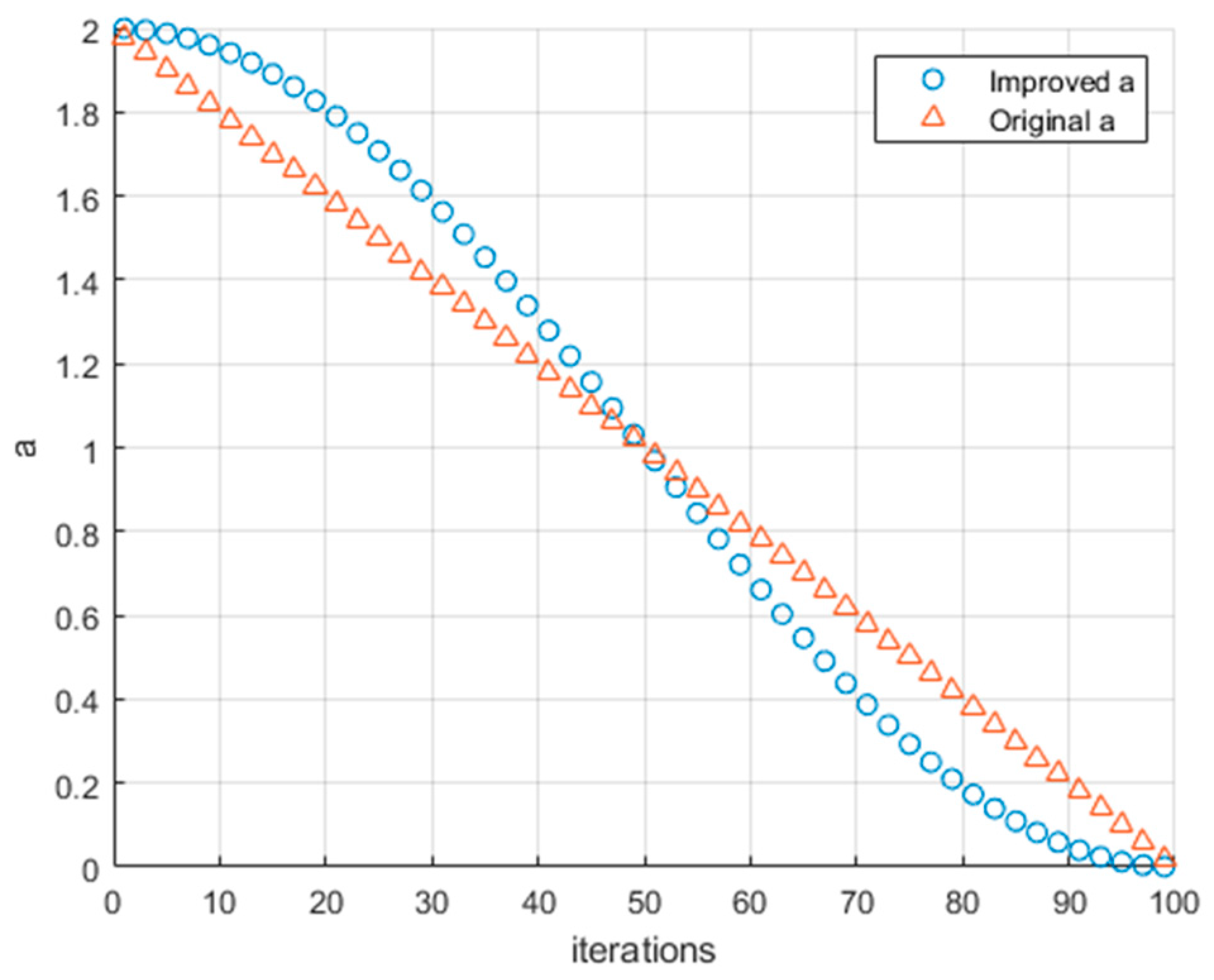
2.2. Nonlinear Convergence Factor

In the GWO algorithm, $A$ is an important parameter that controls the hunting behavior of the grey wolf population. The following equations were proposed in order to simulate the encircling behavior of grey wolves during hunting [14].

$$D=C{X}_p\left(t\right)-X\left(t\right),$$

(6)

$$X\left(t+1\right)=X_p\left(t\right)-AD,$$

(7)

where $t$ indicates the current iteration, $X_p$ is the position of the prey, and $X$ is the position vector of a grey wolf. $A$ and $C$ are coefficients, which can be calculated as follows:

$$A=2a{r}_1-a$$

(8)

$$C=2r_2$$

(9)

where $r_1$ and $r_2$ are random numbers in [0, 1]. When $A>1$, the grey wolves tend to perform a wide-range global search; when $A<1$, the grey wolves attack their prey, i.e., perform a local search near the optimal solution. The convergence factor $a$ directly affects the value of parameter $A$. In the original GWO, $a$ decreases linearly from 2 to 0. However, when dealing with complex problems, the linear decrement strategy often leads to insufficient exploration of the search space. It is more efficient for $a$ to maintain a larger value in the early stages for thorough global exploratio, and a smaller value in the later stages to focus on local exploitation and accelerate convergence. Therefore, it theoretically supports a better exploration–exploitation balance. A nonlinear convergence factor $a$ is proposed, expressed as follows:

$$a=1+\mathrm{c}\mathrm{o}\mathrm{s}(\pi t/T_{max})$$

(10)

where $T_{max}$ is the maximum number of iterations. An example of the change in the convergence factor before and after the improvement for $T_{max}=100$ is shown in Figure 3.

2.3. Grey Wolf Hunting with Manta Ray Foraging

In the original GWO algorithm, population information is not fully utilized, as the position update of individuals is guided only by the three leading wolves. This means that grey wolves always surround the leading wolves. Although this method is beneficial for convergence, if the leading wolves fall into a local optimum, the evolution of the population will stagnate. In order to enhance information exchange within the population, a new position update formula (Equation (11)) is designed that is inspired by the Manta Ray Foraging behavior [29]. The first part of the formula improves the capability of searching for the optimal solution, while the second part helps to increase population diversity to avoid premature convergence. The formula is expressed as follows:

$$X\left(t+1\right)=w{\displaystyle \frac{X_1\left(t\right)+X_2\left(t\right)+X_3\left(t\right)}{3}}+a_0\left(1-w\right)$$

$$\left(r_2\left(X_r\left(t\right)-X\left(t\right)\right)+a_0\kappa r_4\left(X_a\left(t\right)-X\left(t\right)\right)\right),$$

(11)

where

$$X_1\left(t\right)=X_a\left(t\right)-A_1{D}_{\alpha },$$

(12)

$$X_2\left(t\right)=X_{\beta }\left(t\right)-A_2{D}_{\beta },$$

(13)

$$X_3\left(t\right)=X_{\delta }\left(t\right)-A_3{D}_{\delta },$$

(14)

$$\kappa =2e^{r_3{\displaystyle \frac{T-t+1}{T}}}\sin \left(2\pi r_3\right),$$

(15)

$$w=\left(w_{max}-w_{min}\right){\displaystyle \frac{t}{T_{max}}}+w_{min},$$

(16)

where $\kappa$ is the weight coefficient, and $r_3$ and $r_4$ are the rand numbers in [0, 1]. $a_0$ is a constant and takes the value of 0.01. $w$ is the inertia parameter, which is determined by two predefined constants, $w_{max}$ and $w_{min}$, which are 1 and 0.6, respectively. In the early stages, individuals have strong social learning abilities, ensuring global optimal position exploration. In the later stages, the focus shifts to local search around the leading wolves, accelerating convergence. The pseudo-code of the improved hunting strategy is presented in

Table 2. The pseudo-code of grey wolf hunting that integrates Manta Ray Foraging.

% Calculate weight factor w and factor b (Equations (15) and (16)) %w = (wmax − wmin) * current_iteration/max_iterations + wmin %b = (max_iterations − current_iteration + 1)/max_iterations $w=\left(w_{max}-w_{min}\right){\displaystyle \frac{t}{T_{max}}}+w_{min}$  $b={\displaystyle \frac{T_{max}-t+1}{T_{max}}}$  $\% \mathrm{Generate} \mathrm{random} \mathrm{vector} \mathrm{r}3 \mathrm{and} \mathrm{calculate} \kappa$ r3 = random_vector(1, num_variables) % $\kappa$ = 2exp(r3 b) sin(2$\pi$r3) $\kappa =2e^{r_3{\displaystyle \frac{T-t+1}{T}}}\mathrm{s}\mathrm{i}\mathrm{n}(2\pi r_3)$ % Select a random individual random_selection = random_individual (population_size) % Update grey wolf position with Manta Ray Foraging (Equations (11)) $\mathrm{Grey} \mathrm{Wolves}[\mathrm{i}].\mathrm{Position}=w{\displaystyle \frac{X_1\left(t\right)+X_2\left(t\right)+X_3\left(t\right)}{3}}+a_0\left(1-w\right)\left(r_2\left(X_r\left(t\right)-X\left(t\right)\right)+a_0\kappa r_4\left(X_a\left(t\right)-X\left(t\right)\right)\right)$ % Boundary checking $\mathrm{Grey} \mathrm{Wolves}[i$$].\mathrm{Position}=\mathrm{apply}\_\mathrm{bounds}(\mathrm{Grey} \mathrm{Wolves}[i$].Position, lower_bound, upper_bound) % Calculate the cost of the new position $\mathrm{Grey} \mathrm{Wolves}[i$$].\mathrm{Cos}\mathrm{t}=\mathrm{evaluate}\_\cos \mathrm{t}(\mathrm{Grey} \mathrm{Wolves}[i$].Position)

.

2.4. Associative Learning for Archive Update

In MOGWO, the external archive stores non-dominated solutions from the population. This mechanism effectively preserves elite information in the early iterations. However, as iterations progress, the number of non-dominated solutions increases rapidly. Although the crowding distance deletion ensures solution quality to some extent, some optimal solutions may still be lost. Additionally, a large number of similar solutions in the later iterations may cause the population to fall into local optima. Therefore, the solution diversity needs to be enhanced by performing perturbation and mutation in the crowded parts of the archive. The associative learning is an update strategy that can improve the exploration performance of algorithms [30]. Therefore, this paper introduces associative learning to update some individuals in the archive, with the formula as follows:

$$\begin{gathered} X\left(t+1\right)=X\left(t\right)+0.001G\left(X\left(t\right)-lb,ub-X\left(t\right)\right)+b_0{S}_1{r}_1\left(X_r\left(t\right)-X\left(t\right)\right) \\ +b_0{S}_2{r}_2\left(X_P\left(t\right)-X\left(t\right)\right) \end{gathered}$$

(17)

where $r_1$ and $r_2$ are random numbers between 0 and 1, $X_P\left(t\right)$ is the current optimal solution (understood as the $\alpha$ wolf), and $X_r$ denotes a random leader from the preceding generation. $b_0$ is a constant, and $S_1$ and $S_2$ are adaptive cognitive and social factors calculated as follows:

$$S_1=(1-t/T_{max})$$

(18)

$$S_2=2(t/T_{max})$$

(19)

As iterations increase, the value of the adaptive cognitive parameter $S_1$ increases to reduce the impact of the random leader on the search pattern of wolves. On the other hand, the value of $S_2$ increases to enhance the impact of the leader wolf. The rule is designed to approach the optimal value by learning from other wolves and the leader simultaneously. The pseudo-code of associative learning for archive update is presented in

Table 3. The pseudo-code of associative learning for archive update.

% Dominance relationships, archiving, grid updates Determine domination among Grey Wolves Extract non-dominated wolves from Grey Wolves and store in non_dominated_wolves % Add non-dominated wolves to the archive Archive = Archive + non_dominated_wolves % Randomly updating archive using associative learning Archive_num = size_of(Archive) Archive = Associative_Rep(fobj, Archive, gamma, lb, ub, current_iteration, max_iterations, num_variables, Archive_num, Alpha) Determine domination among Archive Extract non-dominated solutions from Archive % Update grid index for each solution in the archive For each solution in Archive: Calculate GridIndex and GridSubIndex for the solution End For % Ensure archive size does not exceed maximum If size_of(Archive) > Archive_size: EXTRA = size_of(Archive) − Archive_size Delete EXTRA solutions from Archive using parameter gamma /% Recalculate costs and update grid Archive_costs = calculate_costs(Archive) G = create_hypercubes(Archive_costs, nGrid, alpha) End If

.

The flowchart in Figure 4 explains how the improved multi-objective grey wolf optimizer (IMOGWO) works for solving multi-objective optimization problems. It begins by initializing the population using Bloch coordinates of qubits and creating an archive of non-dominated solutions. Parameters ($a$), ($A$), and ($C$) are updated, followed by selecting $\alpha$, $\beta$, and $\delta$ wolves using roulette wheel selection. The GWO update mechanism integrates the Manta Ray Foraging behavior to enhance exploration and exploitation. The algorithm then calculates fitness, performs boundary checking, and updates the archive with the associative learning method. This iterative process continues until the stopping criteria are met, ensuring diverse and optimal solutions.

3. Results and Discussion

3.1. Evaluation of Benchmark Functions

3.1.1. Experimental Setup

Table 4. The information on the benchmark functions.

Problem	Pareto-Optimal Front	Number of Objectives	Constraint Condition
ZDT1	convex	2	$m=30;0\le x_i\le 1$
ZDT2	concave	2	$m=30;0\le x_i\le 1$
ZDT3	discontinuous	2	$m=30;0\le x_i\le 1$
Viennet2	discontinuous	3	$m=2;-4\le x,y\le 4$
Viennet3	continuous	3	$m=2;-30\le x,y\le 30$

lists the details of five benchmark functions, comprising three two-objective [30] and two three-objective problems [31]. For the two-objective problems, each of them has 30 dimensions. For the three-objective problems, each of them has two dimensions. The true Pareto-optimal front includes four categories: convex, concave, continuous, and discontinuous.

The Pareto-optimal front of the ZDT1 benchmark problem is known to be convex. The specific form is

$$ZDT1=\left\{\begin{array}{c}{f}_1\left(x\right)=x_1\\ f_2\left(x\right)=g\left(x\right)⌊1-\sqrt{x_1/g\left(x\right)}⌋\\ where g\left(x\right)=1+9\left({\sum }_{i=2}^{30}{x}_i\right)/(30-1)\\ s.t. 0\le x_i\le 1, i=1,2,\dots ,30\end{array}\right.$$

(20)

The Pareto-optimal front of the ZDT2 function exhibits a concave shape. The specific form is

$$ZDT2=\left\{\begin{array}{c}{f}_1\left(x\right)=x_1\\ f_2\left(x\right)=g\left(x\right)⌊1-{\left({\displaystyle \frac{x_1}{g\left(x\right)}}\right)}^2⌋\\ where g\left(x\right)=1+9\left({\sum }_{i=2}^{30}{x}_i\right)/(30-1)\\ s.t. 0\le x_i\le 1, i=1,2,\dots ,30\end{array}\right.$$

(21)

Due to the presence of a sine component in its objective function, ZDT3 exhibits a Pareto front with multiple discontinuities. The specific form is

$$ZDT3=\left\{\begin{array}{c}{f}_1\left(x\right)=x_1\\ f_2\left(x\right)=g\left(x\right)⌊1-\sqrt{{\displaystyle \frac{x_1}{g\left(x\right)}}}-{\displaystyle \frac{x_1}{g\left(x\right)}}\mathrm{s}\mathrm{i}\mathrm{n}(10\pi x_1)⌋\\ where g\left(x\right)=1+9\left({\sum }_{i=2}^{30}{x}_i\right)/(30-1)\\ s.t. 0\le x_i\le 1, i=1,2,\dots ,30\end{array}\right.$$

(22)

The Viennet2 and Viennet3 have a discontinuous and continuous Pareto-optimal front, respectively. The objective functions are described as

$$Viennet2=\left\{\begin{array}{c}F=(f_1\left(x,y\right),f_2\left(x,y\right),f_3(x,y\left)\right)\\ f_1\left(x,y\right)=0.5\times {\left(x-2\right)}^2+{\displaystyle \frac{{(y+1)}^2}{13}}+2\\ f_2\left(x,y\right)={\displaystyle \frac{{(x+y-3)}^2}{36}}+{\displaystyle \frac{{(-x+y+2)}^2}{8}}-17\\ f_3\left(x,y\right)={\displaystyle \frac{{(x+2y-1)}^2}{175}}+{\displaystyle \frac{{(2y-x)}^2}{17}}-13\\ s.t.-4\le x,y\le 4\end{array}\right.$$

(23)

$$Viennet3=\left\{\begin{array}{c}F=(f_1\left(x,y\right),f_2\left(x,y\right),f_3(x,y\left)\right)\\ f_1\left(x,y\right)=0.5\times \left(x^2+y^2\right)+\sin (x^2+y^2)\\ f_2\left(x,y\right)={\displaystyle \frac{{(3x-2y+4)}^2}{8}}+{\displaystyle \frac{{(x-y+1)}^2}{27}}+15\\ f_3\left(x,y\right)={\displaystyle \frac{1}{\left(x^2+y^2+1\right)}}-1.1\exp (-x^2-y^2)\\ s.t.-30\le x,y\le 30\end{array}\right.$$

(24)

A well-solved multi-objective optimization problem is characterized by a Pareto-optimal solution set that both approximates the true front closely and exhibits a high degree of uniformity. In order to quantitatively evaluate the performance of the proposed optimization algorithm in convergence and coverage, four performance indicators are selected, which are defined as follows [32]:

Generational distance (GD): The distance between the calculated Pareto front (${PF}_{know}$) and the optimal Pareto front (${PF}_{true}$), which is an index of the convergence evaluation.

$$GD={\displaystyle \frac{{\left({\sum }_{i=1}^n{d}_i^2\right)}^{\frac{1}{2}}}{n}}$$

(25)

where $n$ is the number of solutions in ${PF}_{know}$. $d_i$ is the Euclidean distance between the i-th solution in the target space and the nearest solution in ${PF}_{true}$. The smaller the $GD$ value, the closer the found non-dominated solution set is to the real non-dominated solution set.

Spacing ($SP$): This measure reflects the extent to which the obtained solutions are evenly distributed in proximity to the actual Pareto front. The definition formula of the $SP$ index is

$$SP=\sqrt{{\displaystyle \frac{1}{n-1}}{\sum }_{i=1}^n{(\overline{d}-d_i)}^2}$$

(26)

where $d_i={}_j{}^{min}\left|f_m^i\left(x\right)-f_m^j\left(x\right)\right|i,j=1,2,\dots ,n$, $i\ne j$; $n$ is the number of solutions in ${PF}_{know}$, which represents the Euclidean distance between the solution closest to itself in the same dimensional objective function. $\overline{d}$ is the average value of $d_i$. $m$ is the target dimension. A lower $SP$ value indicates a better distribution of the obtained solutions.

Inverse generational distance ($IGD$): The metric is designed to simultaneously measure the algorithm’s convergence toward the Pareto front and the diversity of the obtained solutions. The definition formula of $IGD$ is as follows:

$$IGD={\displaystyle \frac{{\sum }_{i=1}^n{d}_i}{n}}$$

(27)

where $d_i$ is the Euclidean distance between the corresponding elements of ${PF}_{true}$ and ${PF}_{know}$. $n$ is the number of true Pareto optimal solutions. The smaller the $IGD$ value, the better the convergence and diversity of the obtained solution set.

The Hypervolume (HV) indicator is used to calculate the hypervolume of a non-dominated set and space reference point and then evaluate the degree to which the ${PF}_{true}$ is covered by ${PF}_{know}$. The reference point can be found by constructing a vector of the worst objective function values. Therefore, HV can be calculated as follows [33]:

$$HV=volume\left({\bigcup }_{si=1}^{\left|Q\right|}{v}_{si}\right)$$

(28)

Here, $Q$ is the solution set of the non-dominant solution front, and $\left|Q\right|$ is the number of non-dominant solution elements. For each non-dominated solution $si\in Q$, a hypercube $v_{si}$ is composed of reference points and members $si$. A higher HV value reflects a broader coverage of the objective space by the Pareto solution set, indicating better algorithmic performance.

3.1.2. Discussion of the Results

Since the grid mechanism and selection leader component maintain the diversity of the archive during optimization [13], three parameters were selected ($Grid\alpha$: grid inflation parameter, $Grid\beta$: leader selection pressure parameter, and $Gridn$: number of grids per each dimension) to perform a sensitivity analysis before evaluating the performance of the IMOGWO. Figure 5 illustrates the variation of three performance metrics—IGD, Spacing, and HV—with respect to different values of these parameters. In the left subplot, changes in $Grid\alpha$ (from 0.05 to 0.15) show that both IGD and Spacing achieve optimal values around $Grid\alpha$ = 0.1, indicating that this setting offers a good balance between solution spread and convergence accuracy. HV remains relatively stable, suggesting the algorithm’s robustness to small variations in this parameter.

In the center subplot, increasing the leader selection pressure $Grid\beta$ from 2 to 6 results in a sharp decline in HV and an increase in IGD and Spacing. This suggests that excessive pressure on the best solutions can reduce diversity and lead to premature convergence. Overall, the results demonstrate that the IMOGWO maintains stable and high-quality performance within a reasonable range of parameter values, with optimal settings around $Grid\alpha$ = 0.1, $Grid\beta$= 4, and $Gridn$= 10.

In the right subplot, the number of grid divisions $Gridn$ has a more pronounced effect. Increasing $Gridn$ from 4 to 12 significantly improves IGD and Spacing, implying enhanced selection granularity and improved leader discrimination. However, overly fine grid resolution (e.g., $Gridn$ = 16) may lead to slight performance degradation, likely due to overfitting the selection process.

In order to evaluate the performance of the IMOGWO, three algorithms (the non-dominated sorting genetic algorithm II (NSGA II), multi-objective grey wolf optimizer (MOGWO), and multi-objective multi-verse optimizer (MOMVO)) are selected for comparison. The maximum iterations are set by $(D\ast \mathrm{10,000})/N$, where $D$ and $N$ represent the dimensions of the problem and the population size, respectively [2]. The value of $N$ is currently set to 100. Figure 6 shows the true and calculated Pareto-optimal fronts of four multi-objective algorithms for ZDT1, which is a convex problem. Generally, the calculated Pareto-optimal fronts of the IMOGWO and MOMVO are much closer to the true Pareto-optimal fronts compared to those of MOGWO and NSGA II. MOGWO can only obtain a few solutions on the true Pareto-optimal front, which indicates there is still room for MOGWO to improve the convergence accuracy. MOMVO can only get several discrete optimal solutions, which means it fails to search the whole solution space. Solutions obtained by NSGA II are far away from the true Pareto-optimal front. Therefore, the IMOGWO can obtain the true Pareto front of ZDT1, which shows the best performance of the four algorithms.

Figure 7 shows the true and calculated Pareto-optimal fronts of four multi-objective algorithms for ZDT2, which is a concave problem. The performance of the IMOGWO and MOMVO is also better than that of MOGWO and NSGA II. MOGWO and NSGA II cannot even capture the shape of the true Pareto-optimal front. The results of MOGWO cluster in a small region of the first objective, which indicates the archive updating fails to search the whole solution space. In addition, NSGA II obtains a convex Pareto-optimal front. For MOMVO, it can only obtain part of the true Pareto front, which in turn demonstrates that using associative learning is able to enhance the diversity of solution sets. Although the calculated Pareto-optimal front of the IMOGWO has a margin of error in certain regions, it still outperforms the other algorithms.

Figure 8 shows the true and calculated Pareto-optimal fronts of four multi-objective algorithms for ZDT3, which has a number of disconnected Pareto-optimal fronts. The IMOGWO provides the best performance dealing with the ZDT3 benchmark function. Although MOGWO can capture the disconnected feature, the error between the true and calculated Pareto-optimal front is relatively large. So, it has a problem of convergence accuracy. For NSGA II, it shows a Pareto-optimal front with a large error. This might be due to the difficulties of the search space of ZDT3 with a number of discontinuous regions that prevent algorithms from providing accurate results on this test problem. Another reason is that the 30-dimensional version of ZDT3 makes it more challenging for multi-objective algorithms. From the above three benchmark functions, the MOMVO has the same problem that it cannot search the whole solution space. Taking advantage of Manta Ray Foraging and associative learning helps to increase population diversity to avoid premature maturation and falling into local optima, which makes the IMOGWO the best performer in these three benchmark functions. Furthermore, it obviously improves the convergence accuracy compared with MOGWO.

In order to further evaluate the performance of the proposed IMOGWO, another two three-objective benchmark functions (Vinnet2 and Vinnet3) are selected, they correspond to a discontinuous and continuous problem, respectively. For Vinnet2, both the IMOGWO and MOGWO work well, as shown in Figure 9. IMOGWO outperforms MOGWO in convergence accuracy, but MOGWO outperforms the IMOGWO in the range of optimal solution search. MOMVO can only find a few optimal solutions, this is the same as the two-objective benchmark functions. Although it has been proven that it has good performance for up to three-objective optimization problems, this algorithm still has room for the improvement of its optima searching ability. As for NSGA II, it does not work for Vinnet2.

As for Vinnet3, the IMOGWO captures the true Pareto-optimal front quite well, as shown in Figure 10. The Pareto-optimal front obtained by MOGWO shifts away from the true Pareto-optimal front, which demonstrates poor convergence accuracy. NSGA II can only obtain part of the true Pareto-optimal front. As regards MOMVO, it lacks a diversity of populations, which restricts the capability of the global search. So far, by comparing the calculated and true Pareto-optimal front, the IMOGWO has shown an improvement in global search and convergence accuracy. Now, in order to obtain the statistical characteristics of four algorithms, each algorithm has to be run 20 times independently. Figure 11 shows the boxplot of the statistical results for the performance metrics (GD, IGD, Spacing, and HV), which are employed to quantitatively analyze convergence and coverage.

In Figure 11, GD and IGD show that all Pareto-optimal fronts obtained by the IMOGWO are close to the true Pareto-optimal fronts, which indicates the IMOGWO has the best convergence accuracy. The performance of NSGA II is the worst. The statistical results of Spacing show that Pareto-optimal fronts obtained by MOMVO have better distribution coverage. However, the Spacing range is large. Therefore, it is not very robust compared with the IMOGWO, especially for ZDT3. Finally, HV proves that the IMOGWO has the best comprehensive performance. So, for two-objective optimization problems (ZDT1-3), the performance of these four algorithms can be ranked as follows: IMOGWO > MOMVO > MOGWO > NSGA II.

Figure 12 presents the statistical results of three benchmark functions for four algorithms. The values of the GD and IGD indicate the IMOGWO has better convergence accuracy compared with MOGWO. Although NSGA II has a small Spacing value, which implies it has a better distribution coverage of the Pareto-optimal front, the GD and IGD show a larger error between the calculated and true Pareto-optimal front. MOMVO shows a highly competitive convergence; however, the results have a poor distribution coverage. Therefore, the IMOGWO still outperforms the other algorithms overall. For the three-objective optimization problem (Vinnet2–3), the performance of these four algorithms can be ranked as follows: IMOGWO > MOMVO > MOGWO > NSGA II.

Furthermore,

Table 5. The statistical results of spread for the different optimization algorithms.

.		IMOGWO	MOGWO	NSGA II	MOMVO			IMOGWO	MOGWO	NSGA II	MOMVO
ZDT1	max	1.144	1.119	0.986	1.023	Viennet2	max	1.144	1.438	0.994	1.294
	min	0.638	0.788	0.968	0.738		min	0.989	0.860	0.992	0.997
	mean	0.876	0.971	0.975	0.872		mean	1.072	1.089	0.993	1.123
	std	0.158	0.111	0.006	0.089		std	0.057	0.171	0.001	0.124
ZDT2	max	1.439	1.216	0.987	1.067
	min	0.773	0.734	0.968	0.830
	mean	1.103	0.996	0.976	0.933
	std	0.253	0.120	0.007	0.076
ZDT3	max	1.044	1.218	1.000	1.948	Viennet3	max	1.360	0.987	1.190	1.724
	min	0.749	0.911	0.975	0.819		min	0.940	0.556	0.850	1.002
	mean	0.906	1.072	0.985	1.503		mean	1.203	0.834	0.980	1.323
	std	0.105	0.089	0.007	0.431		std	0.139	0.136	0.116	0.274

presents the statistical results of the spread metric for the four algorithms—IMOGWO, MOGWO, NSGA II, and MOMVO—across five benchmark problems: ZDT1–ZDT3 and Viennet2–Viennet3. The spread metric measures the uniformity of solution distribution along the Pareto front, where lower values indicate better distribution quality. The IMOGWO demonstrates competitive and stable performance, particularly on ZDT1 (mean = 0.876), ZDT2 (mean = 1.103), and Viennet2 (mean = 1.072), where it achieves both a relatively low mean and standard deviation. Notably, on Viennet3, the IMOGWO outperforms the other methods in terms of both mean spread (1.203) and stability (std = 0.139), suggesting its ability to maintain good diversity on more complex landscapes. Compared to its predecessor MOGWO, the IMOGWO exhibits lower standard deviations across all problems, indicating improved robustness in maintaining spread. While MOMVO shows strong performance in certain cases (e.g., Viennet3), its larger standard deviations (e.g., std = 0.274) point to less consistent diversity control. These results confirm that the IMOGWO achieves a good trade-off between convergence and diversity.

Figure 13 presents a comparison of computing time between the proposed IMOGWO and the original MOGWO across five multi-objective benchmark problems: ZDT1, ZDT2, ZDT3, Viennet2, and Viennet3. For the relatively simple problems (ZDT1–ZDT3), both algorithms exhibit low and comparable computational costs, with the IMOGWO requiring only slightly more time due to additional steps such as Bloch coordinate initialization and archive perturbation. On the more complex test problems (Viennet2 and Viennet3), the computing time increases significantly for both methods due to the increased dimensionality and function complexity. Importantly, although the IMOGWO introduces several enhancements to improve convergence and diversity, its computational time remains close to that of MOGWO, with a moderate decrease observed. This confirms that the proposed modifications maintain computational efficiency while offering performance improvements, making the algorithm suitable for practical multi-objective optimization tasks.

3.2. Aerodynamic Optimization with IMOGWO

3.2.1. Definition of Optimization Problem

The multi-objective optimization process coupled with the IMOGWO algorithm is presented in Figure 14. Firstly, 10 design variables are chosen and used to realize the blade parametrization, which is shown in

Table 6. Definition of the design variables.

No.	Design Variable	Description	Range
1	S_mid	Sweep at mid span	−15%~+15%
2	S_tip	Sweep at blade tip	−15%~+15%
3	T_mid	Twist at mid span	−5%~+5%
4	T_tip	Twist at blade tip	−5%~+5%
5	L_mid	Lean at mid span	−30%~+30%
6	L_tip	Lean at blade tip	−30%~+30%
7	Th_mid	Thickness at mid span	−10%~+10%
8	Th_tip	Thickness at blade tip	−10%~+10%

, and the Latin hyper-cube sampling method is applied to generate 100 design samples that consist of the initial DoE (design of experiment) database. Then, each blade is meshed and evaluated by CFD, and ANSYS CFX^® (V2022R1) is adopted in this paper.

After all design samples have been evaluated, a response surface model (RSM) is built, and the IMOGWO is applied to search for the optimal solutions on the RSM model. Eight Pareto optimum sets are selected and validated by CFD again; if they meet the predefined objectives or reach the final number of iterations, the iterative loop will stop. Otherwise, the eight Pareto sets will be added to the existing samples, and a new RSM model will be regenerated. Through continuous iteration to improve the accuracy of the RSM model, it can contribute to the whole optimization process.

Figure 15 shows the CFD mesh and boundary domains for the single passage. H-type mesh elements are generated using ANSYS TurboGrid^® (V2022R1). An average y+ of less than five is constrained on the blade surfaces and endwalls for low-Reynolds turbulence wall function modeling. The shear stress transport (k-ω SST) turbulence model is used for turbulence closure with a high-resolution advection scheme and first-order discretization. Convergence is achieved when monitoring points achieve stability; specifically, the RMS residuals fall below 1 × 10⁻⁴ and the imbalances of energy, momentum, and mass in all domains are below 0.05% [34].

There are two objectives in the optimization problem: pressure rise ($P_r$) and total pressure efficiency (${Eff}_{tp}$). They are expressed as follows:

$$P_r=Area\_avg\left(P_{out}\right)-Area\_avg\left(P_{in}\right)$$

(29)

$${Eff}_{tp}={\displaystyle \frac{{TP}_r\times VFR}{Q_{input}}}\times 100\%$$

(30)

where ${TP}_r=Mass\_avg\left(P_{out}\right)-Mass\_avg\left(P_{in}\right)$. $P_r$ and ${TP}_r$ are the pressure and total pressure difference, respectively, VFR represents the volume flow rate, and $Q_{input}$ indicates the input shaft power.

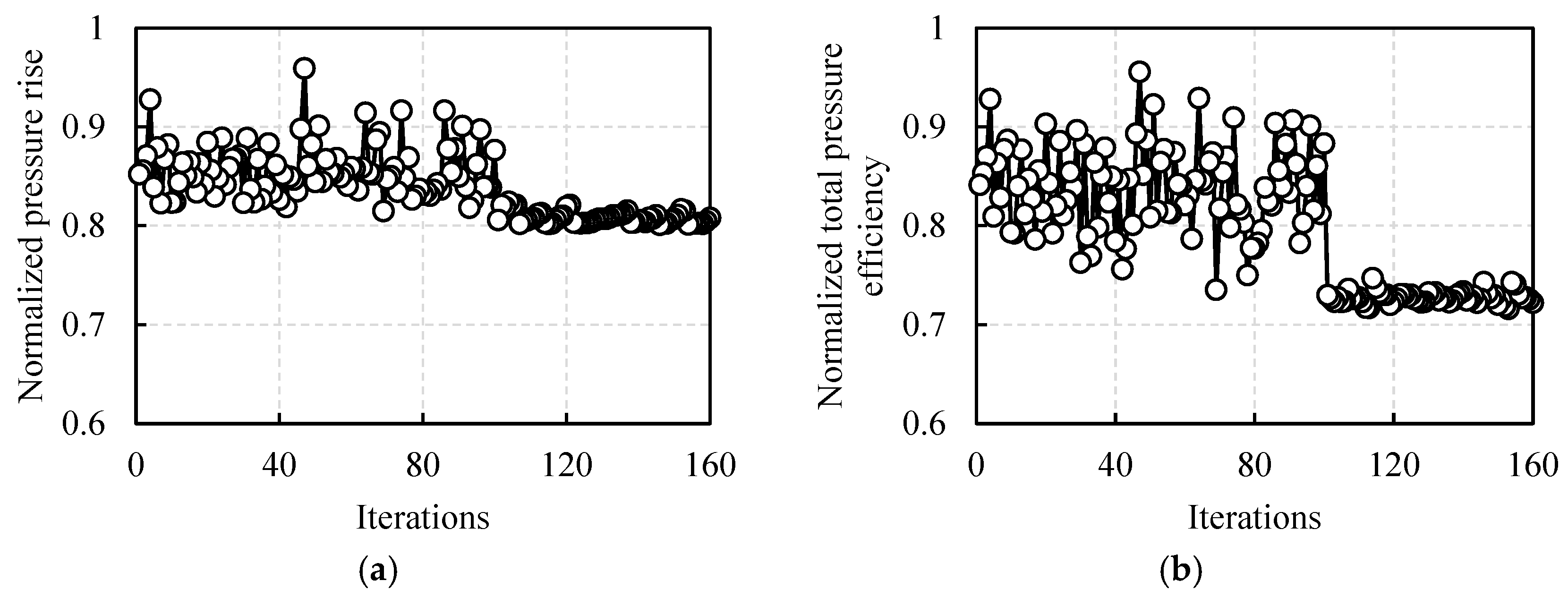
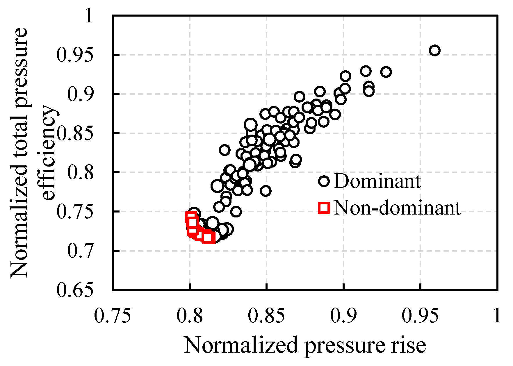
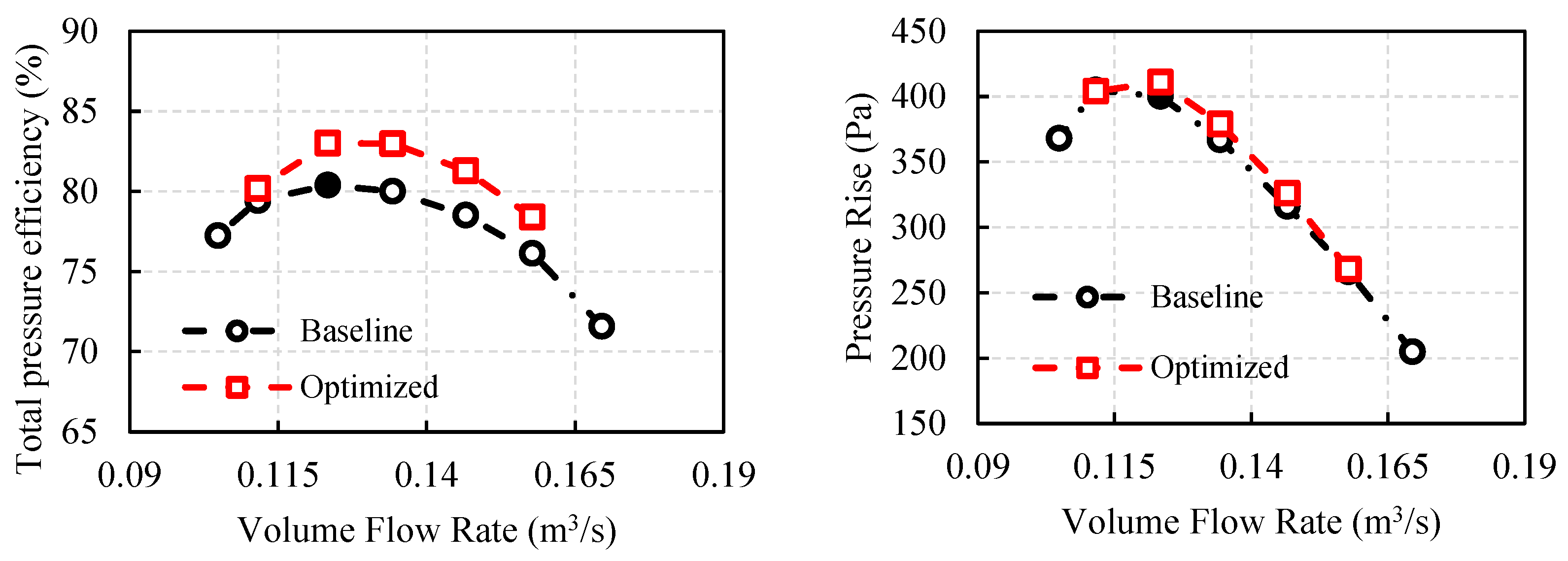
3.2.2. Optimization Results

Figure 16 gives the convergence history of the normalized pressure rise ($\overline{p_r}$) and total pressure efficiency ($\overline{\eta }$). For the convenience of optimization, it should be noted that the normalized pressure rise and total pressure efficiency are defined as shown in Equations (31) and (32) and minimized in the optimization process. Conversely, the pressure rise and total pressure efficiency can be improved.

$$\overline{p_r}={\displaystyle \frac{420-P_r}{420}}$$

(31)

$$\overline{\eta }={\displaystyle \frac{1-{Eff}_{tp}}{0.22}}$$

(32)

It can be found that after eight iterations, the iteration loop ends. The improvement of total pressure efficiency is more obvious than pressure rise. In addition, Figure 17 shows the Pareto-optimal front regarding the aerodynamic performance of the cooling fan obtained by the IMOGWO. The non-dominant solutions are clustering in the lower right corner. Therefore, the proposed IMOGWO algorithm, by generating a diverse set of high-quality non-dominated solutions, enables more flexible and informed decision-making. Rather than providing a single optimal design, it offers a spectrum of viable solutions across the Pareto front, allowing decision-makers to choose configurations that best meet industrial priorities such as cost constraints, performance targets, or manufacturability.

The aerodynamic performance of the baseline and optimized design is presented in Figure 18. In the stable region (0.12–0.16 m³/s), the total pressure efficiency and pressure rise have been improved. At the design point (black dot), the optimized total pressure efficiency is increased by 3.2%, and the pressure rise is increased by 2.75%.

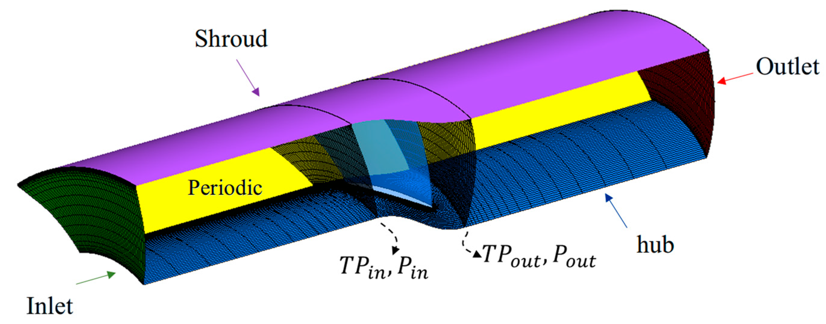
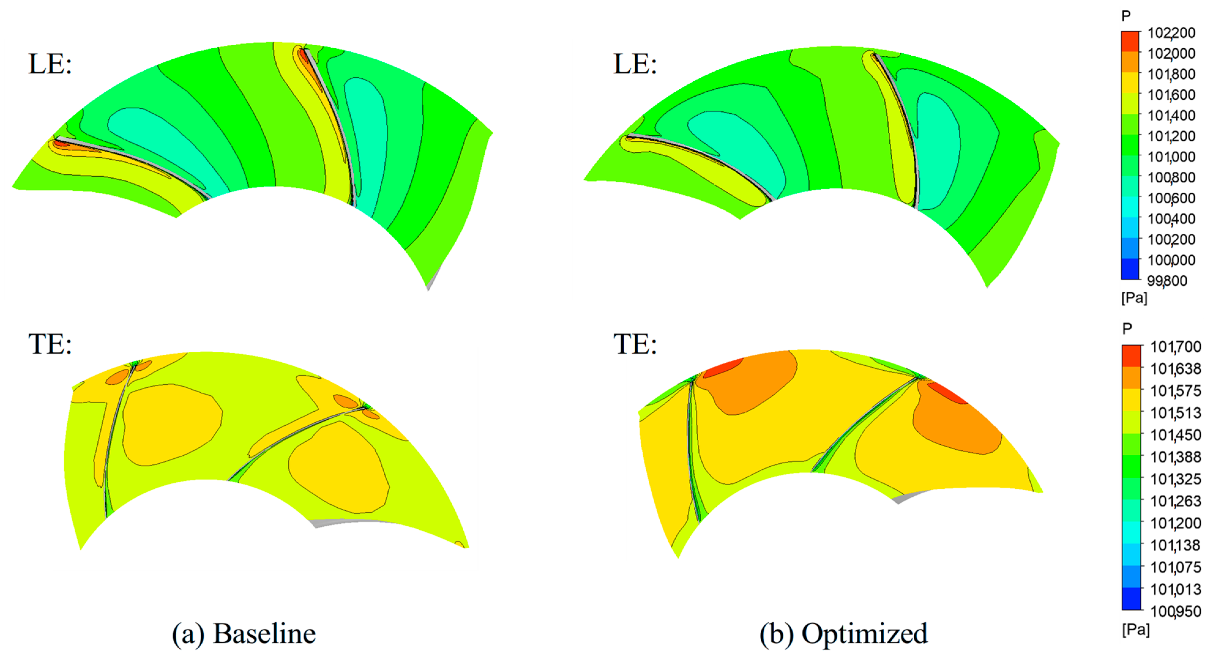
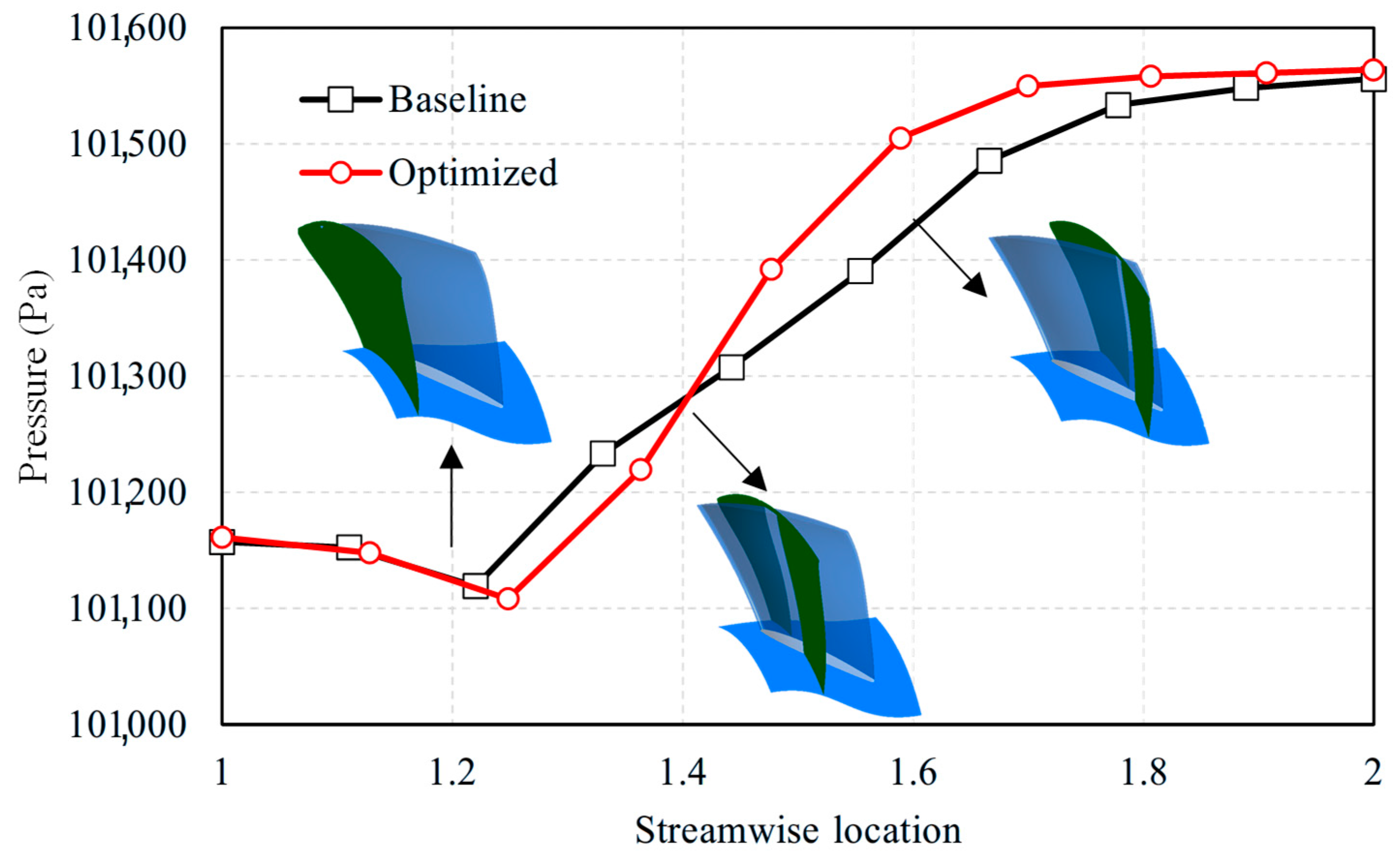
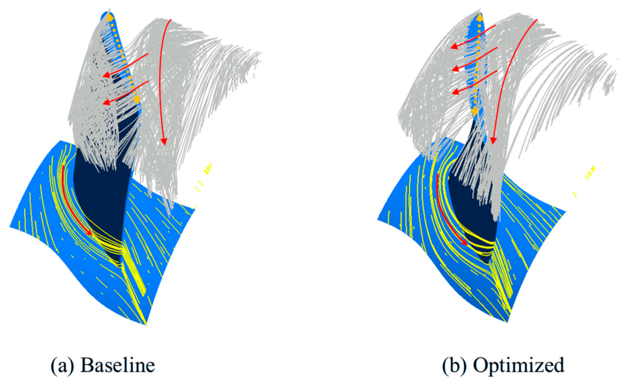
3.2.3. Flow Field Analysis

Figure 19 shows the pressure distributions of the baseline and optimized designs at the leading edge (LE) and trailing edge (TE). The pressure distributions at the LE of the baseline and optimized blades are almost similar. While at TE, it is clear to see that the high-pressure region is increased, especially close to the suction surface, so that the pressure rise of the optimized design improved. This is mainly due to the forward lean near the blade mid-span.

Furthermore, from the pressure distribution along the streamwise location as shown in Figure 20, it can be found that the optimized blade has a higher value of pressure after streamwise location 1.4, which is around a 45% chord length. In the streamwise location ranging from 1.2 to 1.4, the pressure value of the baseline is a little higher. At the inlet, the pressure values of the baseline and optimized designs are almost equal, which is consistent with the pressure distribution in Figure 19.

Figure 21 shows 3D streamlines near the blade root and tip. Since the blade geometry at the blade root is not modified, the flow behavior does not change significantly. Due to the forward lean at the blade mid-span, it enhances the interaction between the tip leakage flow and adjacent blades. That is a reason why the unstable point of the optimized blade moves to a higher volume flow rate, as shown in Figure 18.

4. Conclusions

This paper proposed an improved multi-objective optimization method based on MOGWO. Firstly, the Bloch coordinates of qubits were used to improve the quality of distribution of initial populations over the search space. Then, a modified convergence factor and hunting strategy were used to upgrade the global search ability and convergence. Finally, by taking advantage of the associative learning method, the diversity of solution sets was enhanced to avoid falling into local optima. The IMOGWO was evaluated using five multi-objective benchmark functions and applied to the aerodynamic optimization of a cooling fan. The main conclusions can be drawn as follows:

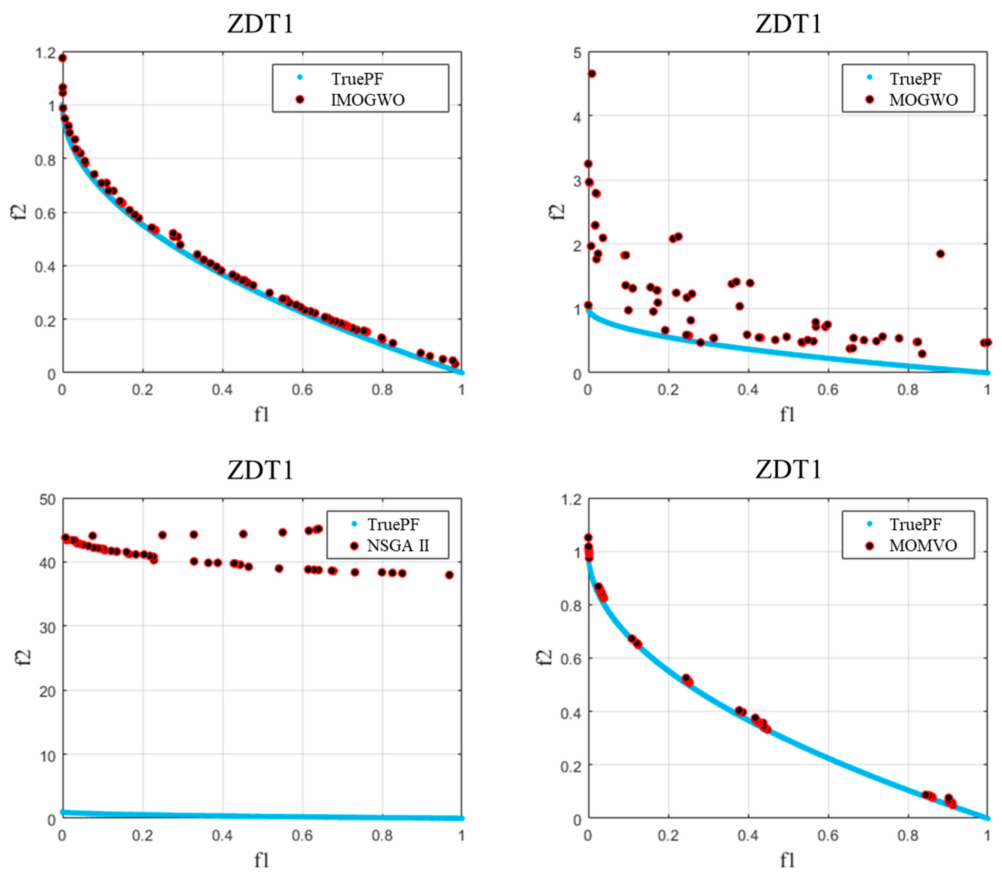
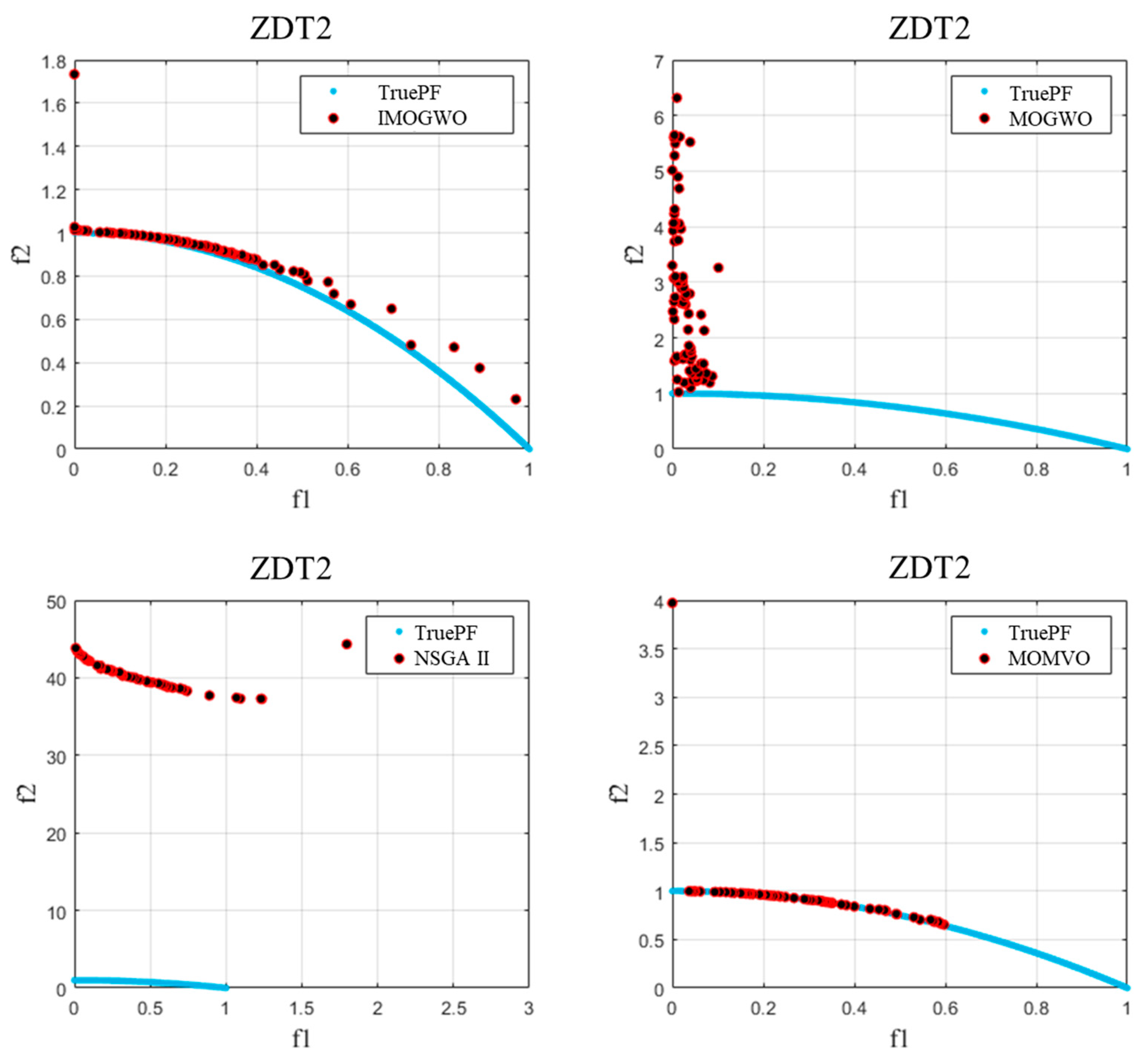
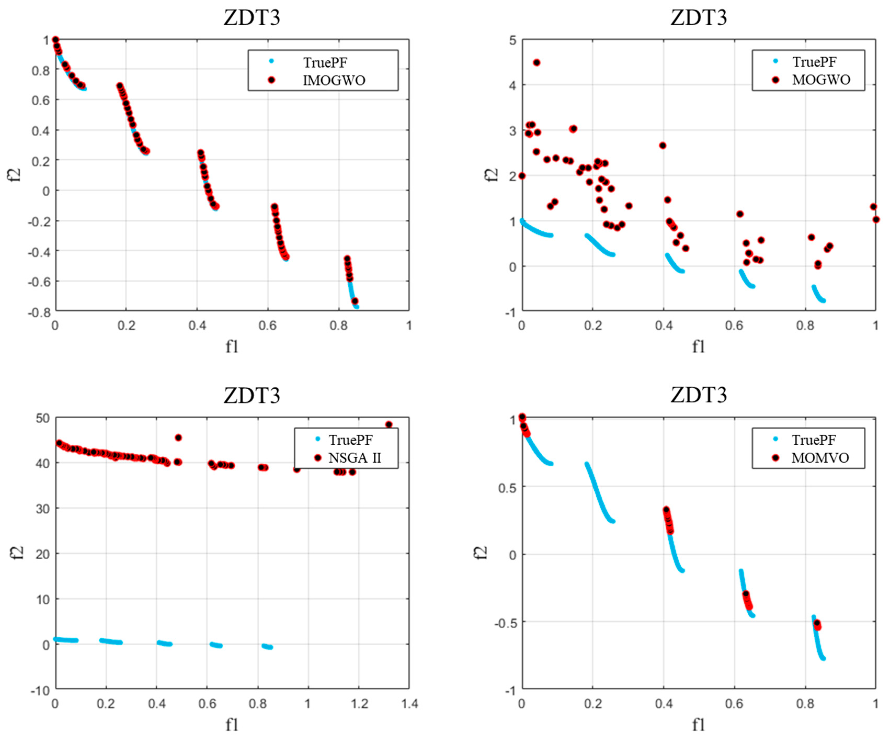
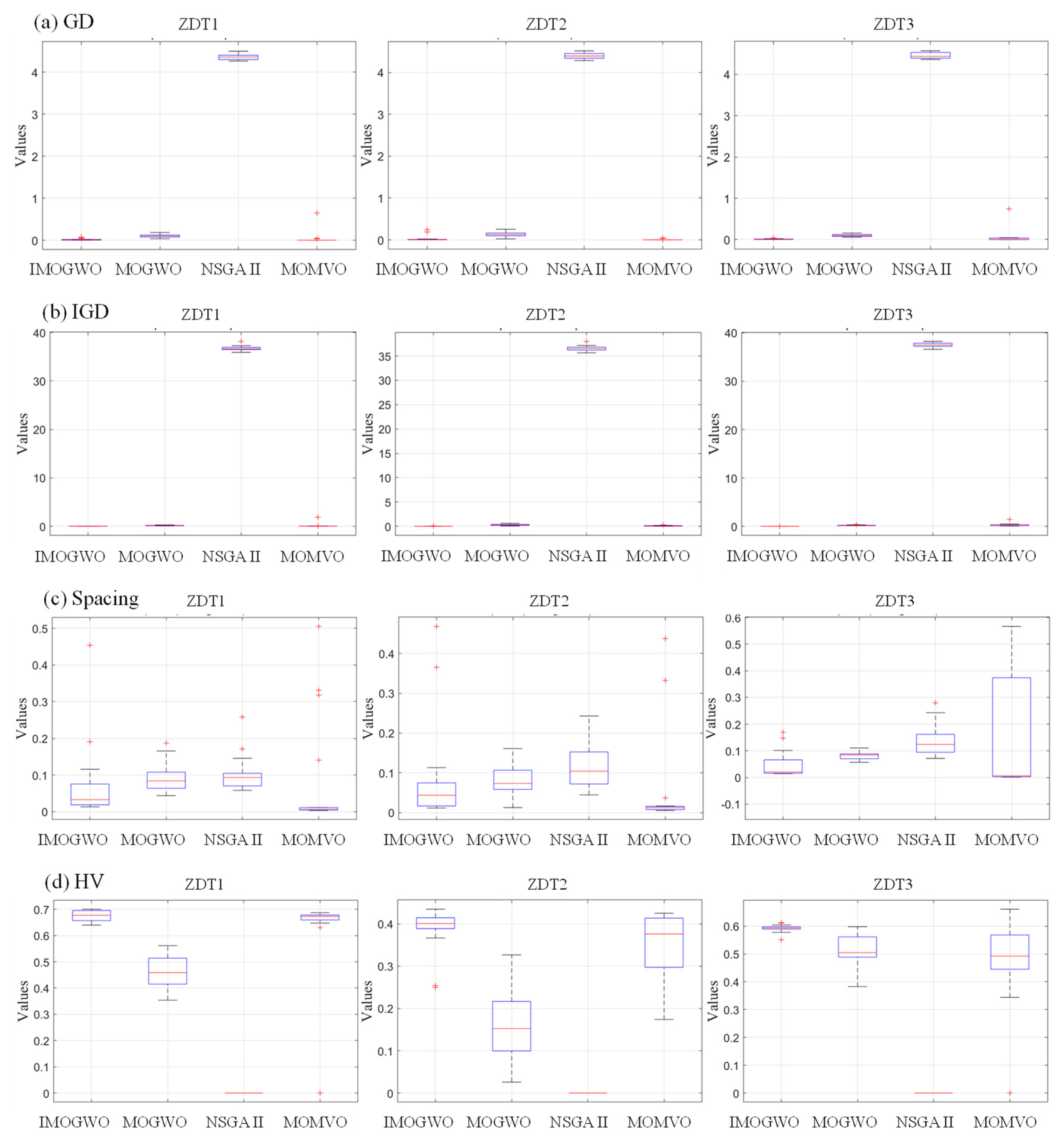
• For two-objective benchmark functions (ZDT1–3), the four performance indicators (GD, IGD, Spacing, and HV) demonstrated that the IMOGWO exhibited enhanced performance in the approximation of the true Pareto-optimal compared with MOGWO, NSGA II, and MOMVO for convex, concave, and discontinuous optimization problems. The analysis results showed that the superiority of the IMOGWO originated from improved exploration and exploitation capabilities.
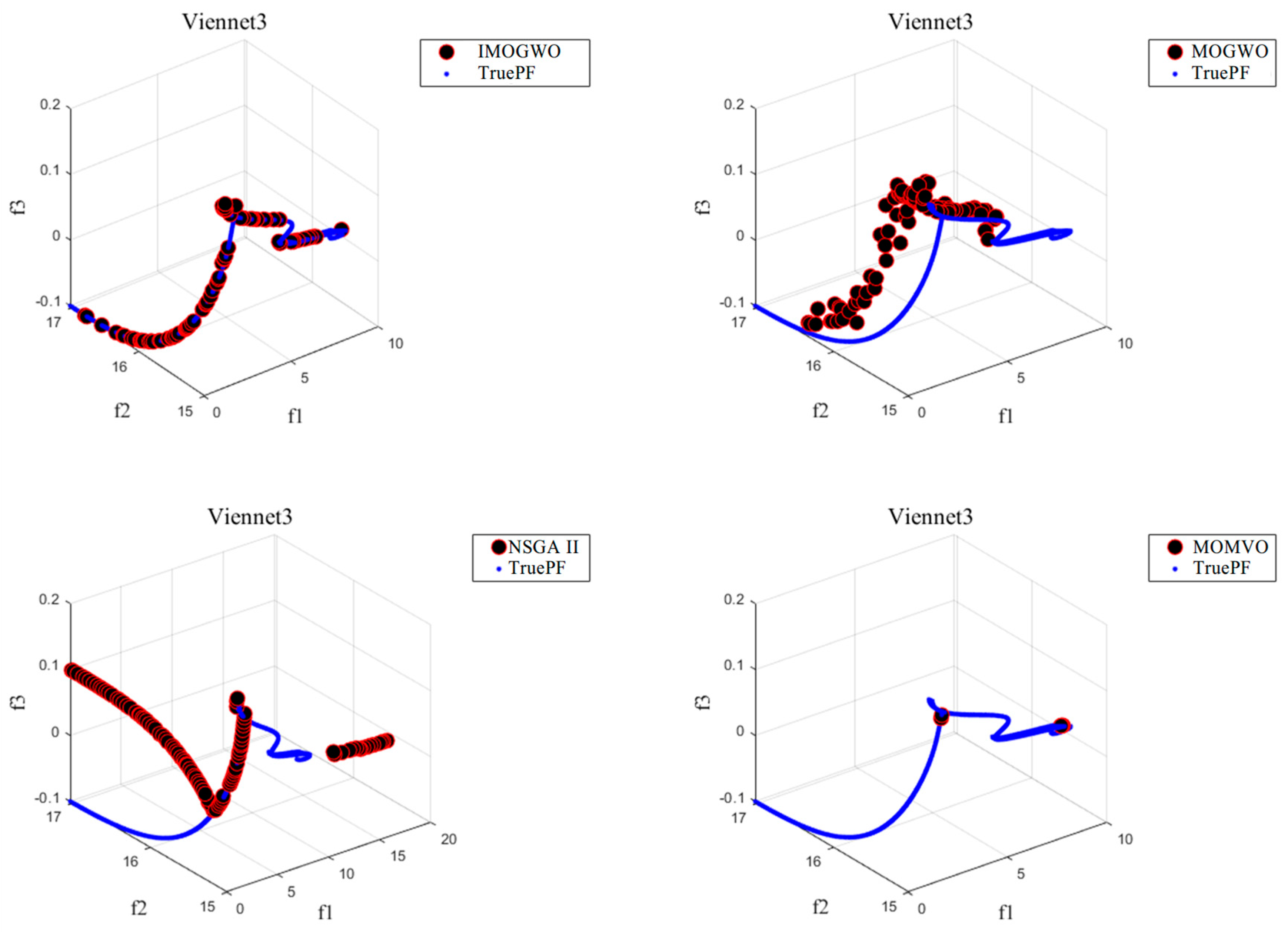
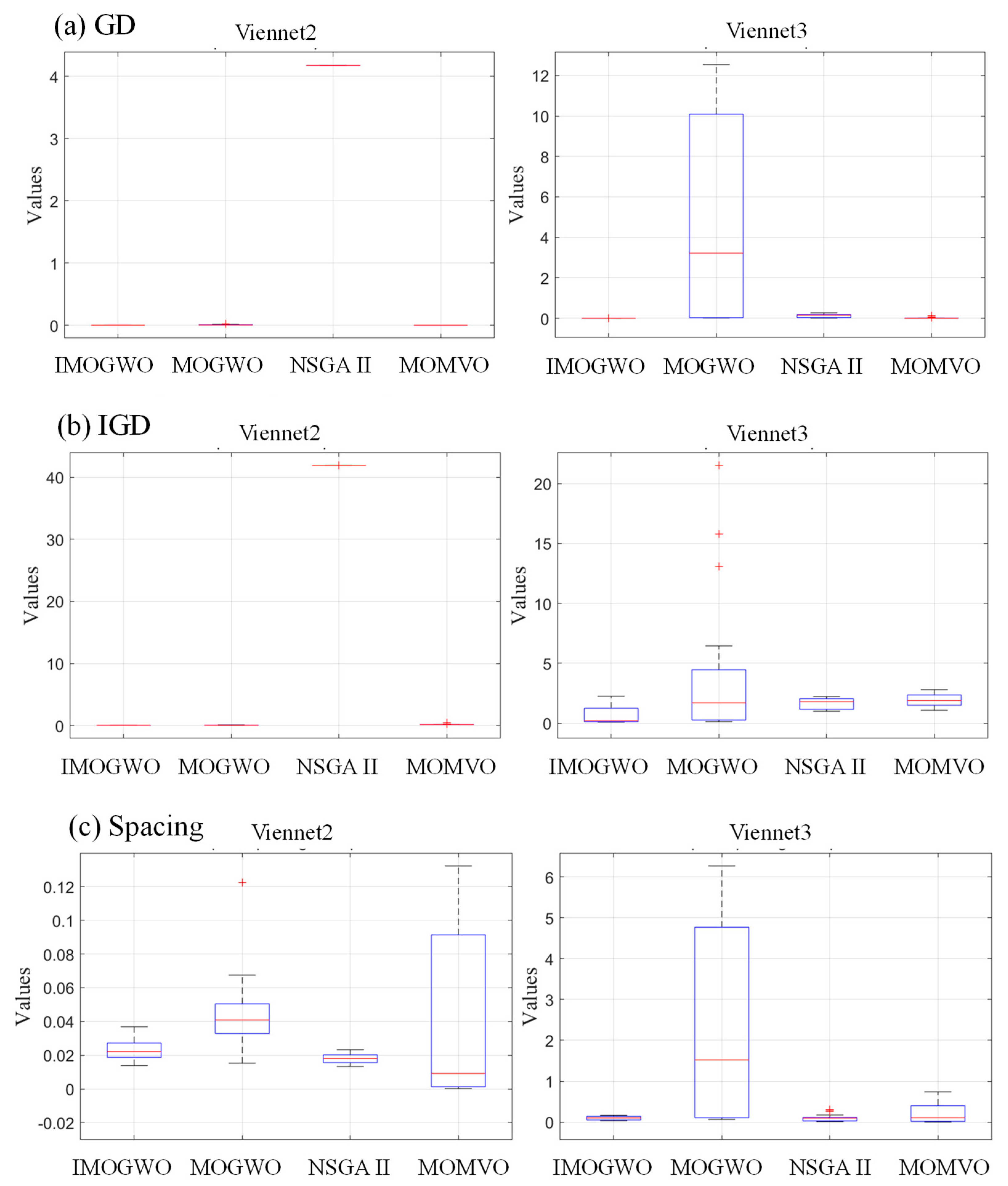
• For three-objective benchmark functions (Vinnet2 and Vinnet3), the three performance indicators (GD, IGD, and Spacing) generally also proved the IMOGWO outperforms MOGWO, NSGA II, and MOMVO. The IMOGWO has an improvement in convergency accuracy and coverage. It can deal with both continuous and discontinuous optimization problems efficiently.
• The multi-objective optimization method integrated with CFD and the IMOGWO increased the total pressure efficiency and pressure rise by 3.2% and 2.75%, respectively, at the design point. It implied that the proposed IMOGWO was able to solve real engineering problems.

For future studies, it is planned to further explore the potential capabilities of the IMOGWO in solving more complex benchmark functions (such as four-objective optimization problems) and develop adaptive parameter control mechanisms to evaluate hybridization with other optimization frameworks. In addition, although the computational cost is reduced compared with the original MOGWO, it may still limit scalability in real-world engineering problems with higher complexity and scalability demands. Therefore, it is also important to further improve computational efficiency.

References

1. Hashim, F.A.; Hussien, A.G. Snake Optimizer: A novel meta-heuristic optimization algorithm. Knowl.-Based Syst. 2022, 242, 108320. [Google Scholar] [CrossRef]
2. Nadimi-Shahraki, M.H.; Taghian, S.; Mirjalili, S. An improved grey wolf optimizer for solving engineering problems. Expert Syst. Appl. 2021, 166, 113917. [Google Scholar] [CrossRef]
3. Kalyanmoy, D.; Amrit, P.; Sameer, A.M.T. A Fast and Elitist Multiobjective Genetic Algorithm: NSGA-II. IEEE Trans. Evol. Comput. 2002, 6, 182–197. [Google Scholar]
4. Deb, K.; Jain, H. An Evolutionary Many-Objective Optimization Algorithm Using Reference-Point-Based Nondominated Sorting Approach, Part I: Solving Problems with Box Constraints. IEEE Trans. Evol. Comput. 2014, 18, 577–601. [Google Scholar] [CrossRef]
5. Shen, J.; Tang, S.; Ariffin, M.K.A.M.; As’Arry, A.; Wang, X. NSGA-III algorithm for optimizing robot collaborative task allocation in the internet of things environment. J. Comput. Sci. 2024, 81, 102373. [Google Scholar] [CrossRef]
6. Fan, M.; Chen, J.; Xie, Z.; Ouyang, H.; Li, S.; Gao, L. Improved multi-objective differential evolution algorithm based on a decomposition strategy for multi-objective optimization problems. Sci. Rep. 2022, 12, 21176. [Google Scholar] [CrossRef]
7. Hassanzadeh, H.R.; Rouhani, M. A Multi-Objective Gravitational Search Algorithm. In Proceedings of the 2010 2nd International Conference on Computational Intelligence, Communication Systems and Networks, Liverpool, UK, 28–30 July 2010; pp. 7–12. [Google Scholar]
8. Junsittiwate, R.; Srinophakun, T.R.; Sukpancharoen, S. Multi-objective atom search optimization of biodiesel production from palm empty fruit bunch pyrolysis. Heliyon 2022, 8, e09280. [Google Scholar] [CrossRef]
9. Beirami, A.; Vahidinasab, V.; Shafie-Khah, M.; Catalão, J.P. Multiobjective ray optimization algorithm as a solution strategy for solving non-convex problems: A power generation scheduling case study. Int. J. Electr. Power Energy Syst. 2020, 119, 105967. [Google Scholar] [CrossRef]
10. Jangir, P.; Mirjalili, S.Z.; Saremi, S.; Trivedi, I.N. Optimization of problems with multiple objectives using the multi-verse optimization algorithm. Knowl.-Based Syst. 2017, 134, 50–71. [Google Scholar] [CrossRef]
11. Coello, C.A.C.; Toscano-Pulido, G.T.; Lechuga, M.S. Handling multiple objectives with particle swarm optimization. IEEE Trans. Evol. Comput. 2004, 8, 256–279. [Google Scholar] [CrossRef]
12. Pradhan, P.M.; Panda, G. Solving multiobjective problems using cat swarm optimization. Expert Syst. Appl. 2012, 39, 2956–2964. [Google Scholar] [CrossRef]
13. Mirjalili, S.; Saremi, S.; Mirjalili, S.M.; Coelho, L.d.S. Multi-objective grey wolf optimizer: A novel algorithm for multi-criterion optimization. Expert Syst. Appl. 2016, 47, 106–119. [Google Scholar] [CrossRef]
14. Gaidhane, P.J.; Nigam, M.J. A hybrid grey wolf optimizer and artificial bee colony algorithm for enhancing the performance of complex systems. J. Comput. Sci. 2018, 27, 284–302. [Google Scholar] [CrossRef]
15. Vijay, R.K.; Nanda, S.J. A Quantum Grey Wolf Optimizer based declustering model for analysis of earthquake catalogs in an ergodic framework. J. Comput. Sci. 2019, 36, 101019. [Google Scholar] [CrossRef]
16. Panwar, K.; Deep, K. Transformation operators based grey wolf optimizer for travelling salesman problem. J. Comput. Sci. 2021, 55, 101454. [Google Scholar] [CrossRef]
17. Nadimi-Shahraki, M.H.; Taghian, S.; Mirjalili, S.; Zamani, H.; Bahreininejad, A. GGWO: Gaze cues learning-based grey wolf optimizer and its applications for solving engineering problems. J. Comput. Sci. 2022, 61, 101636. [Google Scholar] [CrossRef]
18. Al-Tashi, Q.; Abdulkadir, S.J.; Rais, H.M.; Mirjalili, S.; Alhussian, H.; Ragab, M.G.; Alqushaibi, A. Binary Multi-Objective Grey Wolf Optimizer for Feature Selection in Classification. IEEE Access 2020, 8, 106247–106263. [Google Scholar] [CrossRef]
19. Lu, C.; Xiao, S.; Li, X.; Gao, L. An effective multi-objective discrete grey wolf optimizer for a real-world scheduling problem in welding production. Adv. Eng. Softw. 2016, 99, 161–176. [Google Scholar] [CrossRef]
20. Sreenu, K.; Malempati, S. Aggressive Packet Combining Scheme with Packet Reversed and Packet Shifted Copies for Improved Performance. IETE J. Res. 2018, 65, 141–147. [Google Scholar]
21. Sreenu, K.; Malempati, S. FGMTS: Fractional grey wolf optimizer for multi-objective task scheduling strategy in cloud computing. J. Intell. Fuzzy Syst. 2018, 35, 831–844. [Google Scholar] [CrossRef]
22. Yang, Y.; Yang, B.; Wang, S.; Jin, T.; Li, S. An enhanced multi-objective grey wolf optimizer for service composition in cloud manufacturing. Appl. Soft Comput. 2020, 87, 106003. [Google Scholar] [CrossRef]
23. Liu, J.; Yang, Z.; Li, D. A multiple search strategies based grey wolf optimizer for solving multi-objective optimization problems. Expert Syst. Appl. 2020, 145, 113134. [Google Scholar] [CrossRef]
24. Javidsharifi, M.; Niknam, T.; Aghaei, J.; Mokryani, G.; Papadopoulos, P. Multi-objective day-ahead scheduling of microgrids using modified grey wolf optimizer algorithm. J. Intell. Fuzzy Syst. 2019, 36, 2857–2870. [Google Scholar] [CrossRef]
25. Eappen, G.; Shankar, T. Multi-Objective Modified Grey Wolf Optimization Algorithm for Efficient Spectrum Sensing in the Cognitive Radio Network. Arab. J. Sci. Eng. 2020, 46, 3115–3145. [Google Scholar] [CrossRef]
26. Zhang, Z.; Xu, T.; Zou, K.; Tan, S.; Sun, Z. Multi-Objective Grey Wolf Optimizer Based on Improved Head Wolf Selection Strategy. In Proceedings of the 43rd Chinese Control Conference (CCC), Kunming, China, 28–31 July 2024; pp. 1922–1927. [Google Scholar]
27. Liu, J.; Liu, Z.; Wu, Y.; Li, K. MBB-MOGWO: Modified Boltzmann-Based Multi-Objective Grey Wolf Optimizer. Sensors 2024, 24, 1502. [Google Scholar] [CrossRef] [PubMed]
28. Liu, X.; Liu, X. Quantum Particle Swarm Optimization Based on Bloch Coordinates of Qubits. In Proceedings of the 2013 Ninth International Conference on Natural Computation (ICNC), Shenyang, China, 23–25 July 2013. [Google Scholar]
29. Zhao, W.; Zhang, Z.; Wang, L. Manta ray foraging optimization: An effective bio-inspired optimizer for engineering applications. Eng. Appl. Artif. Intell. 2020, 87, 103300. [Google Scholar] [CrossRef]
30. Heidari, A.A.; Aljarah, I.; Faris, H.; Chen, H.; Luo, J.; Mirjalili, S. An enhanced associative learning-based exploratory whale optimizer for global optimization. Neural Comput. Appl. 2019, 32, 5185–5211. [Google Scholar] [CrossRef]
31. Chase, N.; Rademacher, M.; Goodman, E. A benchmark study of multi-objective optimization methods. BMK-3021 Rev 2009, 6, 1–24. [Google Scholar]
32. Li, J.; Guo, X.; Yang, Y.; Zhang, Q. A Hybrid Algorithm for Multi-Objective Optimization—Combining a Biogeography-Based Optimization and Symbiotic Organisms Search. Symmetry 2023, 15, 1481. [Google Scholar] [CrossRef]
33. Liao, Q.; Sheng, Z.; Shi, H.; Zhang, L.; Zhou, L.; Ge, W.; Long, Z. A Comparative Study on Evolutionary Multi-objective Optimization Algorithms Estimating Surface Duct. Sensors 2018, 18, 4428. [Google Scholar] [CrossRef]
34. Adjei, R.A.; Fan, C. Multi-objective design optimization of a transonic axial fan stage using sparse active subspaces. Eng. Appl. Comput. Fluid Mech. 2024, 18, 2325488. [Google Scholar] [CrossRef]
Figure 1. Bloch sphere representation of a qubit.
Applsci 15 05197 g001
Figure 2. The structure of the encoded individual [28].
Applsci 15 05197 g002
Figure 3. A comparison of the original and improved value of a, T m a x = 100 .
Applsci 15 05197 g003
Figure 4. A flow chart of the IMOGWO algorithm.
Applsci 15 05197 g004
Figure 5. The effects of G r i d α , G r i d β , and G r i d n for the IMOGWO and MOGWO.
Applsci 15 05197 g005
Figure 6. The true and calculated Pareto fronts of ZDT1.
Applsci 15 05197 g006
Figure 7. The true and calculated Pareto fronts of ZDT2.
Applsci 15 05197 g007
Figure 8. The true and calculated Pareto fronts of ZDT3.
Applsci 15 05197 g008
Figure 9. The true and calculated Pareto fronts of Vienet2.
Applsci 15 05197 g009
Figure 10. The true and calculated Pareto fronts of Viennet3.
Applsci 15 05197 g010
Figure 11. Boxplot of the statistical results for GD, IGD, Spacing, and HV—two objectives.
Applsci 15 05197 g011
Figure 12. Boxplot of the statistical results for GD, IGD, and Spacing—three objectives.
Applsci 15 05197 g012
Figure 13. A comparison of computing time between the IMOGWO and MOGWO.
Applsci 15 05197 g013
Figure 14. The multi-objective optimization process based on the IMOGWO.
Applsci 15 05197 g014
Figure 15. Single-passage fluid computation domain.
Applsci 15 05197 g015
Figure 16. Convergence history: (a) normalized pressure rise and (b) normalized total pressure efficiency.
Applsci 15 05197 g016
Figure 17. Pareto front calculated by the IMOGWO.
Applsci 15 05197 g017
Figure 18. Aerodynamic performance of the baseline and optimized designs.
Applsci 15 05197 g018
Figure 19. Pressure distributions of the baseline and optimized designs at the LE and TE.
Applsci 15 05197 g019
Figure 20. Comparison of pressure distribution along the streamwise location.
Applsci 15 05197 g020
Figure 21. The 3D streamlines near the blade root and tip.
Applsci 15 05197 g021