Efficient Probabilistic Evaluation and Sensitivity Analysis of Load Supply Capability for Renewable-Energy-Based Power Systems

Abstract

In renewable energy generation, uncertainties mainly refer to power output fluctuations caused by the intermittency, variability, and forecasting errors of wind and photovoltaic power. These uncertainties have adverse effects on the secure operation of the power systems. Probabilistic load supply capability (LSC) serves as an effective perspective for evaluating power system security under uncertainties. Therefore, this paper studies the influence of renewable energy generation on probabilistic LSC to quantify the impact of these uncertainties on the secure operation of the power systems. Global sensitivity analysis (GSA) is introduced for the first time into probabilistic LSC evaluation. It can quantify the impact of renewable energy generation on the system’s LSC and rank the importance of renewable energy power stations based on GSA indices. GSA necessitates multiple rounds of probabilistic LSC evaluation, which is computationally intensive. To address it, this paper introduces a novel probabilistic repeated power flow (PRPF) algorithm, which employs a basis-adaptive sparse polynomial chaos expansion (BASPCE) model as a surrogate model for the original repeated power flow model, thereby accelerating the probabilistic LSC evaluation. Finally, the effectiveness of the proposed methods is verified through case studies on the IEEE 39-bus system. This study provides a practical approach for analyzing the impact of renewable generation uncertainties on power system security, contributing to more informed planning and operational decisions.

1. Introduction

As global attention to environmental protection and sustainable development increases, traditional fossil fuel-based power generation is gradually being replaced by renewable energy sources [1]. The uncertainty introduced by renewable energy generation significantly impacts the security and stability of power systems [2,3]. Load supply capability (LSC) is a crucial aspect of evaluating the security and stability of a power system, as adequate LSC is fundamental to its safe and stable operation [4]. In this view, it is necessary to study how to quantify the influence of renewable energy generation on LSC, which can provide a reference for the planning of renewable energy installations and the real-time dispatch of renewable energy generation.

Many studies have been conducted on the evaluation of the LSC. However, the terms used in these studies are not consistent [5]. In order to avoid confusion, a review of the existing works is provided herein. First of all, the term “load capability”, first introduced in 2000, is defined as the maximum percentage load increase given an arbitrary load growth pattern before encountering electrical or operational constraint violations [6]. In subsequent studies, the concept is also referred to as “available load supply capability (ALSC)” [4,7,8]. More specifically, reference [4] applied the Latin hypercube sampling-Monte Carlo simulation (LHS-MCS) method for a probabilistic evaluation of ALSC. Reference [7] studied the impact of power flow entropy on probabilistic ALSC. Reference [8] combined renewable energy power forecasting with probabilistic ALSC evaluation, achieving probabilistic forecasting of ALSC. Secondly, the term “total supply capability (TSC)”, also called as “power supply capability (PSC)” [9,10], was proposed in 2011 by Xiao et al. [11]. It is defined as the maximum load that a distribution system can provide under the N-1 security criterion. The two main differences between TSC and load capability are that load capability focuses on operational constraints, whereas TSC focuses on N-1 security constraints, and TSC does not specify a load growth pattern. Xiao et al. subsequently conducted a series of studies to supplement and refine the TSC family indices. For instance, reference [5] improved the ASC index within the TSC family, and reference [10] examined the TSC evaluation primarily considering user reliability requirements constraints. The third term is “loadability”, which lacks a unified definition and carries different meanings in various studies. For example, reference [12] defined loadability as a knee or turning point of the power flow solution curve, which can be obtained through a robust two-stage algorithmic framework proposed in the study. In reference [13], loadability refers to the system’s capability to accommodate added load, and it is derived through an optimization procedure. In reference [14], loadability is defined as an index calculated based on network parameters and system states.

In summary, despite the different terms used, studies on LSC consistently aim to determine the maximum load the power system can support. The studies vary by considering different decision variables and constraints tailored to specific scenarios and applications. As for solving algorithms, the optimization problem defined by load capability (also referred to as ALSC) is relatively simple and can be solved using the repeated power flow (RPF) method [4,8]. On the other hand, the problems involving TSC or loadability without a specified load growth pattern are more complex and often solved using the optimal power flow (OPF) method [14]. The continuation power flow (CPF) method is frequently used to address loadability problems that account for static voltage stability constraints [15]. In this paper, ALSC and RPF are chosen because we focus more on operational constraints and computational convenience.

All the above works have made a significant contribution to the evaluation of the LSC. However, there are two main research gaps in the existing studies. The first gap is that no work has studied how to improve the computational efficiency of the probabilistic evaluation of the LSC. 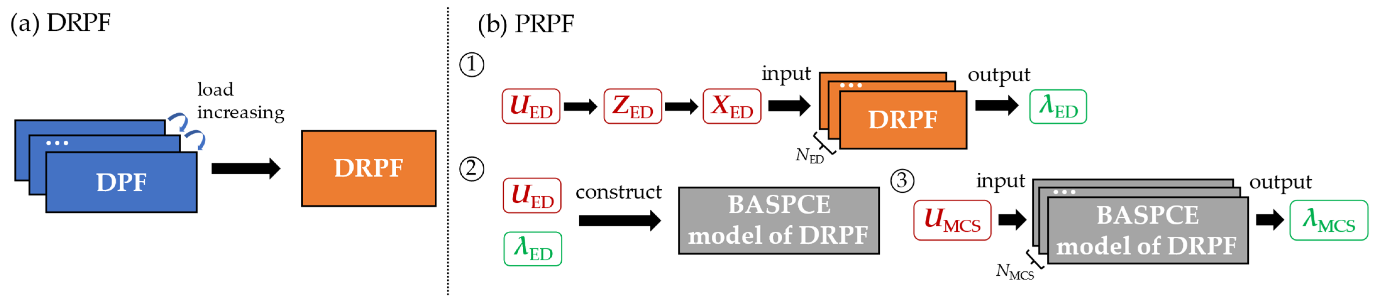In recent years, with the rapid increase in the number of uncertainty sources in power systems, there has been a growing interest in the uncertainty quantification of the LSC evaluation [4,7,8]. As to the authors’ knowledge, most existing works use the simulation methods to calculate the probabilistic RPF (PRPF), which require enormous rounds of deterministic calculations to ensure the convergence. This necessitates significant data storage and computational resources, which are not conducive to real-time grid dispatch and analysis. Therefore, improving the efficiency of probabilistic LSC evaluation is a meaningful but overlooked problem.

Polynomial chaos expansion (PCE) is a commonly used method for enhancing computational efficiency in uncertainty quantification, which has been successfully applied in various fields such as optimal power flow [16], fault location [17], and economic dispatch [18]. The fundamental idea of PCE is to use a set of orthogonal polynomials to approximate the original system model. Basis-adaptive sparse polynomial chaos expansion (BASPCE) is an advanced method that employs the basis-adaptive procedure to automatically select the appropriate truncation strategy and uses a sparse-adaptive scheme to address the curse of dimensionality. Therefore, this paper employs BASPCE to establish a surrogate model for the whole process of the ALSC evaluation to enhance the computational efficiency of probabilistic ALSC evaluation.

The second research gap is that no studies have yet analyzed the impact of renewable energy generation on the system’s LSC. Existing works typically focus on the LSC of the power system or distribution systems, and even though the systems they studied include renewable energy generation, they do not quantify this impact. The inherent uncertainty of renewable energy generation can affect the system’s LSC, making it essential to use specific indices to quantify and evaluate this impact. These indices can also serve as the LSC indices for renewable energy power stations (currently, only the system’s LSC indices exist), providing valuable references for the planning and dispatch of renewable energy generation. In other words, shifting the research focus from the power system to a specific renewable energy power station is highly significant.

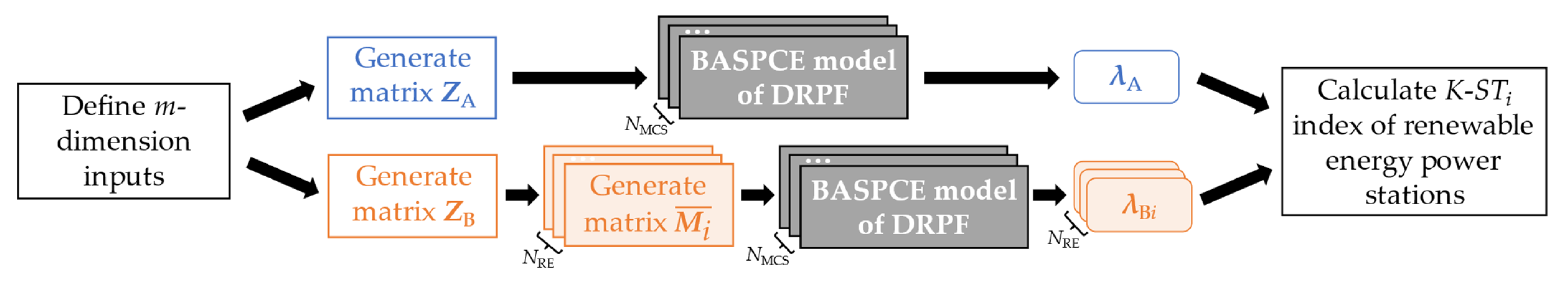
Global sensitivity analysis (GSA) is a method capable of analyzing the impact of renewable energy generation on the system’s LSC. This technique measures the influence of input random variables on the probabilistic characteristics of the target output variable [19,20]. Specifically, the outputs of renewable energy power stations can be considered as input random variables, and their GSA indices can be computed with respect to the LSC. Based on the results of the GSA indices, the importance of each renewable energy power station can be ranked. In engineering practice, specific operational strategies can be formulated for the controllable equipment of the important renewable energy power stations based on these rankings, thereby enhancing the performance of the LSC.

In general, the research aim of this paper is to study the influence of the uncertainties caused by renewable energy generation on the power system’s LSC. The main innovations and contributions of this paper are summarized as follows:

(1)

A novel PRPF method is proposed for the probabilistic evaluation of ALSC. This method works based on BASPCE, which can enhance computational efficiency while holding high accuracy.

(2)

The GSA is introduced systematically into the LSC evaluation to rank the importance of renewable energy power stations in contributing to the system’s LSC.

(3)

To validate the effectiveness of the proposed method, experiments are conducted on the modified IEEE 39-bus system. Various scenarios are designed to analyze the influence of load growth direction and correlation on the test results.

The framework of this paper is as follows. Section 2 introduces the probabilistic modeling of uncertainty sources. Section 3 describes the PRPF method based on BASPCE for the probabilistic evaluation of ALSC. Section 4 presents the GSA method in the probabilistic evaluation of ALSC. The proposed method is verified on the IEEE 39-bus system in Section 5, while conclusions are summarized in Section 6.

2. Probabilistic Modeling of Uncertainty Sources

This paper chooses the probability distribution method [21] for modeling uncertainty sources. Uncertainty modeling of random variables is performed based on measured data. The uncertainty sources in this paper include wind power stations, photovoltaic power stations, and loads.

2.1. Marginal Distribution Modeling of Uncertainty Sources

The calculation formula for the power output forecasting error of uncertainty sources is as follows:

$$\Delta P_{\mathrm{U},t}=P_{\mathrm{U},t}^F-P_{\mathrm{U},t}$$

(1)

where ΔP_U,t is the forecasting error of uncertainty sources at time t; $P_{\mathrm{U},t}^F$ and P_U,t are the power forecasting value and measured value of uncertainty sources, respectively.

Let $f\left(\chi \right)$ be the probability density function of the random variable $\chi$, its kernel density estimation formula is as follows [22]:

$$f(\chi )={\displaystyle \frac{1}{nw}}{\displaystyle \sum _{i=1}^{n}K(\frac{\chi -{\chi }_i}{w})}$$

(2)

where w is bandwidth; K(·) is kernel function; n is sample size; ${\chi }_i$ is the i-th random sample.

2.2. Random Sampling Considering the Correlation of Random Variables

Due to the correlation amongst variables, direct sampling from correlated samples is not feasible. Therefore, this paper first extracts the Spearman rank correlation coefficients from the measured data and then generates random samples that are mutually independent and follow a standard normal distribution; and finally, based on Cholesky decomposition and the equiprobability principle, these samples are converted into random samples that are correlated and follow the original distribution.

When the marginal distribution of the random variables changes, the Spearman rank correlation coefficient in the standard normal domain is equal to the correlation coefficient in the original domain. The relationship between the Pearson correlation coefficient and the Spearman rank correlation coefficient in the standard normal domain is as follows [23]:

$${\rho }_{z_{ij}}=2\sin ({\displaystyle \frac{\pi }{6}}{\rho }_{s,z_{ij}})$$

(3)

where ${\rho }_{z_{\mathrm{ij}}}$ and ${\rho }_{{\mathrm{s},z}_{\mathrm{ij}}}$ are the elements in the i-th row and j-th column of the Pearson correlation coefficient matrix C_z and the Spearman rank correlation coefficient matrix C_s,z in the standard normal domain, where z denotes the standard normal domain.

To generate m × N random sample matrix X = [x₁,x₂,…,x_m]^T, it is first necessary to generate m × N independent standard normal sample matrix U = [u₁,u₂,…,u_m]^T and then convert U into a standard normal sample matrix Z = [z₁,z₂,…,z_m]^T that incorporates the correlation of the measured data [7]:

$$\mathit{Z}=\mathit{L}\mathit{U}$$

(4)

where L is the matrix obtained by performing Cholesky decomposition on the correlation coefficient matrix C_z as follows [24]:

$${\mathit{C}}_z=\mathit{L}{\mathit{L}}^T$$

(5)

Finally, for the k-th dimensional random variables x_k and z_k, the random samples that satisfy the original domain distribution can be obtained according to the following equation [25].

$$x_k=F^{-1}(\Phi (z_k))$$

(6)

where $\Phi$(·) is the standard normal cumulative distribution function; F⁻¹ is the inverse of the original cumulative distribution function.

3. Probabilistic Evaluation of ALSC Based on BASPCE

In this section, we first introduce the deterministic ALSC evaluation, including its mathematical formulation and solution methods. After that, the theories of BASPCE are presented. In the end, the PRPF method based on BASPCE for probabilistic evaluation of ALSC is introduced.

3.1. Deterministic Evaluation of ALSC

The load increasing multiple $\lambda$ can be used to quantify the ALSC. The $\lambda$ is determined by gradually increasing the load until encountering any electrical or operational constraint violation. The deterministic ALSC problem can be mathematically formulated as follows [6]:

Objective:

$$\max \lambda$$

(7)

Subject to:

$$\left\{\begin{array}{l}f(x)+\lambda b=0\\ U_{i\min }\le U_i\le U_{i\max }\\ S_{ij}\le S_{ij\max }\\ P_{Gi}\le P_{Gi\max }\end{array}\right.$$

(8)

where f(x) represents the power flow equation; b is the load growing vector; $U_i$ is the nodal voltage amplitude of bus i; $U_{i \min }$ and $U_{i \max }$ are the minimum and the maximum nodal voltage amplitude limitation of bus i, respectively; $S_{ij}$ is the apparent power of the branch between bus i and bus j, and $S_{ij \max }$ is the maximum apparent power; $P_{\mathrm{G}i}$ is the active power output of the generator at bus i, and $P_{\mathrm{G}i \max }$ is the maximum power output limitation of the generator at bus i.

RPF is a commonly used method for solving deterministic ALSC problems. Its basic principle involves starting from the initial conditions and gradually increasing the load according to a specified load growth pattern, repeatedly performing deterministic power flow (DPF) calculations until any electrical constraint is violated. The detailed calculation steps of deterministic ALSC evaluation by RPF can be found in reference [8].

3.2. Theory of BASPCE [26]

Assume that ξ = [ξ₁,ξ₂,...,ξ_m] is an m-dimensional independent input random vector with a known joint probability density function. Appropriate orthogonal polynomials can be selected corresponding to each input random variable. The original model output response Y_s = g_s(ξ) can then be approximated by the sum of these orthogonal polynomial expansions.

$$g_s(\mathit{\xi })\approx {\displaystyle \sum _{\mathit{\alpha }\in \mathrm{\Theta }}{\gamma }_{\mathit{\alpha }}}{\mathrm{\Psi }}_{\mathit{\alpha }}(\mathit{\xi })$$

(9)

where Θ$\subset {\mathbb{N}}^m$ represents the truncation scheme contained within the m-dimensional natural number spherical domain; Ψ_α(ξ) denotes the multivariate polynomial basis functions; γ_α is the expansion coefficient corresponding to the basis function Ψ_α(ξ).

For the multivariate polynomial basis functions Ψ_α(ξ), they are formed by the tensor product of univariate orthogonal polynomial basis functions.

$${\mathrm{\Psi }}_{\mathit{\alpha }}(\mathit{\xi })={\displaystyle \prod _{i=1}^m{\varphi }_{{\alpha }_i}^{(i)}({\xi }_i)}$$

(10)

where ${\varphi }_{{\alpha }_i}^{\left(i\right)}\left({\xi }_i\right)$ represents the α-th order orthogonal polynomial corresponding to the variable ξ_i.

The choice of the orthogonal polynomial basis function for a given input random variable is related to the type of probability distribution of that variable. The relationship between several classical types of input random variable probability distributions and their corresponding optimal univariate orthogonal polynomial basis functions is shown in Appendix A. For a random variable ξ_i following an arbitrary distribution type, the corresponding univariate orthogonal polynomials can be constructed using the recurrence relation in [27].

For the truncation scheme, the expansion terms in (3) are typically truncated based on a truncation criterion parameter p, resulting in a total number of non-zero terms in the truncated PCE model given by:

$$K^{m,p}=\left(\begin{array}{c}m+p\\ p\end{array}\right)={\displaystyle \frac{(m+p)!}{m!p!}}$$

(11)

This truncation scheme is denoted as Θ^m,p = {$\mathit{\alpha }\in {\mathbb{N}}^m$: |α| ≤ p}, referred to as the standard truncation scheme for generalized PCE. The total number of terms in the truncated expansion is K^m,p + 1. However, not every term in the expansion has a significant impact on the output response; only a subset of the expansion terms corresponding to certain input random variables is crucial, known as the sparsity-of-effects principle. Based on this principle, a hyperbolic truncation scheme can be introduced, which effectively excludes higher-order interaction terms [28].

$${\mathrm{\Theta }}_q^{m,p}=\left\{\mathit{\alpha }\in {\mathrm{\Theta }}^{m,p}:{‖\mathit{\alpha }‖}_q={\left({\displaystyle \sum _{i=1}^m{({\alpha }_i)}^q}\right)}^{{\displaystyle \raisebox{1ex}{$1$}\!\left/ \!\raisebox{-1ex}{$q$}\right.}}\le p,q\in (0,1]\right\}$$

(12)

where q is the truncation norm used to adjust the sparsity. Under this truncation scheme, the total number of terms in the expansion is denoted as K_q^m,p + 1. When q = 1, the hyperbolic truncation is fully equivalent to the standard truncation scheme. When 0 < q < 1, the expansion terms under hyperbolic truncation include all high-order univariate terms but exclude higher-order interaction terms; furthermore, the smaller the value of q, the fewer higher-order interaction terms are included in the expansion.

Additionally, the estimated values of the expansion coefficients γ_α can be determined using the least squares method. By generating a sample set of input random variables {${\mathit{\chi }}_1$,...,${\mathit{\chi }}_{N_{\mathrm{ED}}}$} through random sampling, this set is generally referred to as the experimental design (ED) sample set, and N_ED is the ED sample size. Substituting the obtained ED sample set into the original model allows for the calculation of the corresponding output sample vector Y = [g_s(${\mathit{\chi }}_1$),..., g_s(${\mathit{\chi }}_{N_{\mathrm{ED}}}$)]^T. Thus, the least squares problem for calculating the expansion coefficients can be formulated as follows:

$$\min {\displaystyle \sum _{l=1}^{N_{\mathrm{ED}}}{[g_s({\mathit{\chi }}_l)-{\mathit{\gamma }}^T\mathit{J}({\mathit{\chi }}_l)]}^2}$$

(13)

where γ = [γ₀,…,${\gamma }_{K_q^{m,p}}$]^T represents the coefficient vector under the hyperbolic truncation scheme, and J(${\mathit{\chi }}_{\mathrm{l}}$) = [Ψ₀(${\mathit{\chi }}_{\mathrm{l}}$),…, ${\mathrm{\Psi }}_{K_q^{m,p}}\left({\mathit{\chi }}_l\right)$]^T is the polynomial matrix corresponding to the experimental design sample point χ_l. Let J = [J(${\mathit{\chi }}_1$), J(${\mathit{\chi }}_2$),…, J(${\mathit{\chi }}_l$),…,J(${\mathit{\chi }}_{N_{\mathrm{ED}}}$)]^T, then the solution to (13) can be obtained using the following expression:

$$\widehat{\mathit{\gamma }}={({\mathit{J}}^T\mathit{J})}^{-1}{\mathit{J}}^T\mathit{\gamma }$$

(14)

In order to further reduce the higher-order interaction terms in the expansion under the hyperbolic truncation scheme, a penalty term can be introduced based on (13):

$$\min \left\{{\displaystyle \sum _{l=1}^{N_{\mathrm{ED}}}{[g_s({\mathit{\chi }}_l)-{\mathit{\gamma }}^T\mathit{J}({\mathit{\chi }}_l)]}^2}+\lambda {\displaystyle \sum _{\mathit{\alpha }\in {\mathrm{\Theta }}_q^{m,p}}|{\gamma }_{\mathit{\alpha }}|}\right\}$$

(15)

where λ is the penalty factor. Several algorithms can solve the penalized minimization problem in (15), including the LASSO method [29], forward stagewise regression [30], and least angle regression (LAR) [31], with the LAR method being successfully applied in [32] to obtain sparse PCE models.

To sum up, it is necessary to set the value of p, followed by determining the orthogonal basis functions, selecting the truncation strategy, and calculating the expansion coefficients to build the PCE model. However, the value of p corresponding to the PCE model with acceptable accuracy is typically unknown in advance. Therefore, combining the concept of adaptive algorithms with sparse PCE leads to the development of the BASPCE method. This method aims to select the most suitable value of p by using the leave-one-out (LOO) cross-validation error e_LOO as shown below.

$$e_{\mathrm{L}\mathrm{O}\mathrm{O}}={\displaystyle \frac{{\displaystyle \sum _{l=1}^{N_{\mathrm{ED}}}{(g_s({\mathit{\chi }}_l)-g_s^{\mathrm{PCE}(l)}({\mathit{\chi }}_l))}^2}}{{\displaystyle \sum _{l=1}^{N_{\mathrm{ED}}}{(g_s({\mathit{\chi }}_l)-\frac{1}{N_{\mathrm{ED}}}{\displaystyle \sum _{l=1}^{N_{\mathrm{ED}}}{g}_s({\mathit{\chi }}_l)})}^2}}}$$

(16)

where g_s^PCE(l)(∙) denotes the PCE model constructed based on the new sample set {χ_j: j = 1,2,..., N_ED, j ≠ l}, obtained by removing the l-th sample from the experimental design sample set.

3.3. PRPF Calculation Method Based on BASPCE

In order to conduct the probabilistic evaluation of ALSC, the PRPF method based on BASPCE is proposed. First, it is necessary to construct the BASPCE model of deterministic RPF (DRPF). As illustrated in Figure 1a, DRPF consists of multiple deterministic power flow (DPF) calculations. It is worth noting that the BASPCE model constructed is for DRPF, not for DPF. As shown in Figure 1b. Once the BASPCE model of DRPF is obtained, it can be used to perform PRPF to conduct the probabilistic evaluation of ALSC. Figure 1b illustrates three processes, which are in order: ① obtaining ED samples, ② constructing the BASPCE model, ③ performing PRPF using the BASPCE model. The detailed procedure is outlined as follows:

Procedure 1: PRPF Calculation Method Based on BASPCE

1. Read the parameters of random inputs, including the dimension m, distribution types, and parameters;

2. Generate m × NED sampling matrix XED, during which process, corresponding m × NED independent standard Gaussian distributed matrix UED and m × NED correlated standard Gaussian distributed matrix ZED, as shown in Section 2.2;

3. Execute a batch of DRPFs with XED and obtain the output load increasing multiple matrix ${\mathit{\lambda }}_{\mathrm{ED}}=[{\lambda }_1, {\lambda }_2,\dots ,{\lambda }_{N_{\mathrm{ED}}}$];

4. Construct the BASPCE model with UED and λED;

5. Generate a m × NMCS sampling matrix XMCS of the random inputs, during which process, corresponding UMCS and ZMCS;

6. Execute sampling matrix UMCS through the constructed BASPCE model;

7. Get the results of the probabilistic evaluation of ALSC λMCS.

4. The GSA in Probabilistic Evaluation of ALSC

4.1. Theory of GSA

4.1.1. The Idea of GSA

The ANOVA is introduced in [33] to quantify the contribution of each independent variable X_i (i = 1, 2,…,m) to the variance of the output. This method measures the influence of X_i on the output variable Y_s by the reduction in output variance when X_i is set to a fixed value. When X_i is assigned a specific value x_i*, the conditional variance of the output can be expressed as V(Y_s|X_i = x_i*). Since this conditional variance depends on x_i*, to account for the impact of X_i when it is fixed at all possible values, the expected value of the conditional variance $E_{X_i}\left[V\right(Y_s|X_i\left)\right]$ needs to be calculated. Combining this with the law of total variance from probability and statistics theory:

$$V(Y_s)=V_{X_i}[E(Y_s|X_i)]+E_{X_i}[V(Y_s|X_i)]$$

(17)

The first-order sensitivity index (FSI) of the input variable X_i is defined as follows:

$$S_i={\displaystyle \frac{V(Y_s)-E_{X_i}[V(Y_s|X_i)]}{V(Y_s)}}={\displaystyle \frac{V_{X_i}[E(Y_s|X_i)]}{V(Y_s)}}$$

(18)

In addition, the total sensitivity index (TSI) is defined as follows [34]:

$$S{T}_i={\displaystyle \frac{E_{{\mathit{X}}_{~i}}[V(Y_s|{\mathit{X}}_{~i})]}{V(Y_s)}}=1-{\displaystyle \frac{V_{{\mathit{X}}_{~i}}[E(Y_s|{\mathit{X}}_{~i})]}{V(Y_s)}}$$

(19)

where X_~i represents the vector composed of the remaining m−1 dimensional input random variables, excluding X_i. The first-order sensitivity index S_i reflects the impact of a single variable on the output variance, but it is infeasible to explore the joint effects between different input variables. In contrast, the total sensitivity index ST_i reflects the combined influence of the input variable X_i as well as the interaction between X_i and all other input variables on the output variance. Therefore, the total sensitivity index is the main focus of this paper. These indices are called Sobol indices. More details of the Sobol indices can be found in [26].

4.1.2. The Definition of Kucherenko Index

The Kucherenko index can be considered as the extension of the Sobol indices for the case, where input variables are correlated. Given an m-dimension input random vector X = [X_v, X_w], for any subvector ${\mathit{X}}_{\mathit{v}}=\left[{\mathit{X}}_{i_1},\dots ,{\mathit{X}}_{i_d}\right]$ and its complementary subvector ${\mathit{X}}_w=\left[{\mathit{X}}_{i_{d+1}},\dots ,{\mathit{X}}_{i_m}\right]$, the variance of the output variable Y_s can be decomposed in a manner similar to (17) as follows:

$$g_{s,0}=E(Y_s)={\displaystyle \int g_s(\mathit{X})}\mathrm{d}\mathit{X}$$

(20)

$$V(Y_s)=V_{{\mathit{X}}_v}[E_{{\overline{\mathit{X}}}_w}(Y_s|{\mathit{X}}_v)]+E_{{\mathit{X}}_v}[V_{{\overline{\mathit{X}}}_w}(Y_s|{\mathit{X}}_v)]$$

(21)

$$V_{{\mathit{X}}_v}[E_{{\overline{\mathit{X}}}_w}(Y_s|{\mathit{X}}_v)]={\displaystyle \underset{R^d}{\int }{f}_{{\mathit{X}}_v}({\mathit{x}}_v)}\mathrm{d}{\mathit{x}}_v{\left[{\displaystyle \underset{R^{m-d}}{\int }{g}_s({\mathit{x}}_v,{\overline{\mathit{x}}}_w)f_{{\overline{\mathit{X}}}_w}({\overline{\mathit{x}}}_w|{\mathit{x}}_v)\mathrm{d}{\overline{\mathit{x}}}_w}\right]}^2-g_{s,0}^2$$

(22)

$$E_{{\mathit{X}}_v}[V_{{\overline{\mathit{X}}}_w}(Y_s|{\mathit{X}}_v)]={\displaystyle \underset{R^d}{\int }{f}_{{\mathit{X}}_v}({\mathit{x}}_v)}\mathrm{d}{\mathit{x}}_v{\left[{\displaystyle \underset{R^{m-d}}{\int }{\left(g_s({\mathit{x}}_v,{\overline{\mathit{x}}}_w)\right)}^2{f}_{{\overline{\mathit{X}}}_w}({\overline{\mathit{x}}}_w|{\mathit{x}}_v)\mathrm{d}{\overline{\mathit{x}}}_w-g_{s,0}^2}\right]}^2$$

(23)

where g_s denotes the original model; x_v represents a set of sampling values of the subvector X_v; $f_{{\mathit{X}}_v}\left({\mathit{x}}_v\right)$ is the marginal probability density function of X_v; the complementary subvector under the condition X_v = x_v denoted as ${\stackrel{-}{\mathit{X}}}_w$, and ${\stackrel{-}{\mathit{x}}}_w$ as a set of sampling values of ${\stackrel{-}{\mathit{X}}}_w$.

According to the law of total variance shown in (21), Kucherenko et al. defined the following total sensitivity index (hereafter, it will be referred to as the K-ST index in this paper) [35]:

$$K\text{-}S{T}_i={\displaystyle \frac{E_{{\mathit{X}}_{~i}}[V_{{\overline{X}}_i}(Y_s|{\mathit{X}}_{~i})]}{V(Y_s)}}$$

(24)

4.1.3. Computational Strategy

According to the idea of single-loop Monte Carlo (SMC) [36], Kucherenko et al. provided estimation formula for (24) [35].

$$K\text{-}S{T}_i={\displaystyle \frac{1}{2N_{\mathrm{sam}}\widehat{V}(Y_s)}}{\displaystyle \sum _{j=1}^{N_{\mathrm{sam}}}{\left[g_s({\mathit{x}}^{(j)})-g_s({\overline{x}}_i^{(j)},{\mathit{x}}_{~i}^{(j)})\right]}^2}$$

(25)

where M_A = {${\mathit{x}}^{\left(1\right)}$, ${\mathit{x}}^{\left(2\right)}$…, ${\mathit{x}}^{\left(N_{\mathit{sam}}\right)}$} and M_B = {${\mathit{x}}^{’\left(1\right)}$, ${\mathit{x}}^{’\left(2\right)}$…, ${\mathit{x}}^{’\left(N_{\mathit{sam}}\right)}$} are two different input sample sets generated from the joint probability density function of the input random variables X; ${\stackrel{\mathrm{-}}{\mathit{x}}}_{~i}^{\left(j\right)}$ is generated from the conditional probability density function when $X_i=x_i^{\left(j\right)}$; $\widehat{V}(Y_s)$ is the estimated value of the output variance.

Moreover, when the input variables are correlated, it is necessary to discuss the conditional distribution of the input vector ${\stackrel{\mathrm{-}}{\mathit{X}}}_w$ when X_v takes a fixed value. For simplicity, we first analyze correlated standard normal distribution variables. Assume that the variable Z = [Z₁,..., Z_m] = [Z_i, Z_~i] follows a standard normal distribution with mean vector μ and covariance matrix Σ. The components Z_i and Z_~i also follow standard normal distributions with mean vectors μ_i and μ_~i, and covariance matrices Σ_i and Σ_~i, respectively. Consequently, the mean vector μ and covariance matrix Σ can be expressed as follows:

$$\mathit{\mu }=\left[\begin{array}{c}{\mu }_i\\ {\mathit{\mu }}_{~i}\end{array}\right],\hspace{1em}\Sigma =\left[\begin{array}{cc}{\Sigma }_i& {\mathit{\Sigma }}_{i,~i}\\ {\mathit{\Sigma }}_{~i,i}& {\mathit{\Sigma }}_{~i}\end{array}\right]$$

(26)

Let the variable ${\stackrel{\mathrm{-}}{Z}}_i$ represent the conditional variable when Z_~i takes a fixed value z_~i. Then, the variable ${\stackrel{\mathrm{-}}{Z}}_i$ will follow a normal distribution with a mean ${\stackrel{\mathrm{-}}{\mu }}_i$ and covariance ${\stackrel{\mathrm{-}}{\Sigma }}_i$, where ${\stackrel{\mathrm{-}}{\mu }}_i$ and ${\stackrel{\mathrm{-}}{\Sigma }}_i$ are given by:

$${\overline{\mu }}_i={\mu }_i+{\mathit{\Sigma }}_{~i,i}{\mathit{\Sigma }}_{~i}^{-1}({\mathit{z}}_{~i}-{\mathit{\mu }}_{ ~i})$$

(27)

$${\overline{\mathit{\Sigma }}}_i={\Sigma }_i-{\mathit{\Sigma }}_{i,~i}{\mathit{\Sigma }}_{~i}^{-1}{\mathit{\Sigma }}_{~i,i}$$

(28)

According to (25), to obtain the first-order sensitivity indices and total sensitivity indices corresponding to all input random variables, a total of N_sim = N_MCS + m × N_MCS = (m + 1)N_MCS model evaluations are required, where N_MCS is the Monte Carlo simulation number. Since N_MCS typically needs to be a large value to ensure the convergence of the probabilistic calculation results, the computational burden of the SMC method becomes particularly significant in power system analysis applications with high-dimensional input variables.

4.2. GSA for PRPF Based on BASPCE

GSA is introduced into the PRPF to analyze the global sensitivity of the power of renewable energy power stations on the system’s LSC. Specifically, the K-ST index in Section 4.1.2 is calculated, and based on the magnitude of the K-ST, the importance of renewable energy power stations can be ranked. The BASPCE model is combined with the computational strategy outlined in Section 4.1.3, as shown in Figure 2. The detailed procedure is as follows:

Procedure 2: GSA for PRPF Based on BASPCE

1. Read the parameters of random inputs, including the dimension m, distribution types, and parameters;

2. Generate a m × NMCS matrix ZA and a m × NMCS matrix ZB (correlated standard Gaussian);

3. Execute sampling matrix ZA through the BASPCE model and obtain the output λA;

4. According to (21)–(22) and ZB, generate the conditional sampling matrix $\overline{{\mathit{M}}_i}$ for the i-th input random variables;

5. Execute sampling matrix $\overline{{\mathit{M}}_i}$ through the BASPCE model and obtain the output λBi;

6. According to λA and λBi and (19), calculate the K-STi index for the i-th input random variables; 7. Repeat steps 4 to 6, traversing i from 1 to NRE (number of renewable energy power stations) to calculate the K-ST index for all renewable energy power stations.

5. Test Results and Discussion

In this section, the proposed methods are applied to the modified IEEE 39-bus system in view of the procedure as detailed explained in Section 3. The work is carried out in MATLAB R2023b. The computer used for simulation is equipped with an Intel i5-13400 2.50 GHz CPU at 3.40 GHz with 32 GB RAM. MATPOWER is used to calculate the DPF [37], and toolbox UQLab is adopted for BASPCE [38].

5.1. Test Setups

As shown in Figure 3, two wind power stations are connected to nodes 18 and 19 in the standard IEEE 39-bus system (denoted as W1 and W2), while three photovoltaic (PV) power stations are connected to nodes 23, 24, and 25 (denoted as PV1, PV2, and PV3). The penetration rate of renewable energy is 15%. The detailed information on the renewable energy power station is shown in Appendix B. The base load is increased to 1.2 times the value in the standard IEEE 39-bus system. The uncertainties in the PV and wind power generation, as well as the load, are derived from the data in the Belgian grid dataset [39]. The dataset contains measured and forecasting data for renewable energy power stations and load, from which the forecasting error data can be calculated. Then, non-parametric kernel density estimation can be used to model the marginal distribution of source and load power forecasting errors. The detailed steps for modeling the uncertainty of source and load power can be found in Appendix B. The wind farms are set with a leading power factor of 0.98 [4], the PV power stations are set with zero reactive power [40], and the loads maintain their original power factors. The correlation between loads is set to 0.7 [4], while the other correlations are calculated using the Spearman correlation coefficients based on the Belgian grid dataset. The truncation criterion parameter p of BASPCE is set to 1~6, and the truncation norm q is set to 0.8 [41]. The ED sample size N_ED is 1000. The other parameters setting of the system is shown in Appendix B. The load growth pattern vector in RPF is set as 5% of the base load.

To conduct an in-depth analysis of the experimental results, three different scenarios are designed, as shown in

Table 1. Setting of the test scenarios.

Scenarios	Descriptions
S1	Default setting in Section 5.1.
S2	Penetration rate of renewable energy rises to 30%.
S3	The correlation coefficients among WPS, among PVS, between WPS and loads, between PVS and loads, and between WPS and PVS are set to 0.7, 0.7, −0.2, 0.7, −0.2.

. The penetration rate of renewable energy is a critical issue in modern energy systems. As the development of renewable energy continues, its penetration rate is expected to increase. Therefore, in S2, the installed capacity of each renewable energy station is proportionally scaled up, raising the penetration rate of renewable energy from 15% to 30%, while keeping all other settings consistent with S1. In addition, the correlation among renewable sources, as well as between renewable sources and load, may vary in practice. To investigate the impact of correlation on the results, S3 modifies the correlation coefficients as follows: wind power stations (WPS) and photovoltaic stations (PVS) to 0.7, WPS and load to −0.2, PVS and load to 0.7, and WPS and PVS to −0.2. All other settings in S3 are kept the same as in S1.

5.2. Tests on Accuracy and Efficiency of BASPCE for PRPF

To evaluate the accuracy and computational speed of BASPCE, a total of eight uncertainty quantification methods, as listed in

Table 2. Statistical results of the ALSC evaluation with different methods in S1.

Methods	FHSI/%	${\mathit{\epsilon }}_{\mathit{E}}$/%	${\mathit{\epsilon }}_{\mathit{S}}$/%	T/s	T1/s	T2/s
SRS-MCS 104	97.53	0.04	1.60	1081.14	-	1081.14
LHS-MCS 104	97.74	0.03	2.77	1064.69	-	1064.69
SRS-MCS 103	92.91	0.21	5.29	121.33	-	121.33
LHS-MCS 103	93.84	0.12	4.94	120.16	-	120.16
SRS-BASPCE 104	97.51	0.04	6.00	118.62	118.50	0.12
LHS-BASPCE 104	97.40	0.12	3.63	118.65	118.50	0.15
SRS-BASPCE 105	98.59	0.10	3.53	118.76	118.50	0.26
LHS-BASPCE 105	98.48	0.13	5.58	118.78	118.50	0.28

,

Table 3. Statistical results of the ALSC evaluation with different methods in S2.

Methods	FHSI/%	${\mathit{\epsilon }}_{\mathit{E}}$/%	${\mathit{\epsilon }}_{\mathit{S}}$/%	T/s	T1/s	T2/s
SRS-MCS 104	98.68	0.06	0.93	836.93	-	836.93
LHS-MCS 104	98.47	0.05	0.78	857.27	-	857.27
SRS-MCS 103	93.59	0.22	5.71	88.27	-	88.27
LHS-MCS 103	94.13	0.14	3.25	84.88	-	84.88
SRS-BASPCE 104	98.42	0.05	1.86	84.28	84.14	0.14
LHS-BASPCE 104	98.10	0.10	2.48	84.27	84.14	0.13
SRS-BASPCE 105	98.71	0.11	2.80	84.46	84.14	0.32
LHS-BASPCE 105	99.11	0.09	2.21	84.47	84.14	0.33

and

Table 4. Statistical results of the ALSC evaluation with different methods in S3.

Methods	FHSI/%	${\mathit{\epsilon }}_{\mathit{E}}$/%	${\mathit{\epsilon }}_{\mathit{S}}$/%	T/s	T1/s	T2/s
SRS-MCS 104	97.37	0.16	0.41	892.19	-	892.19
LHS-MCS 104	97.80	0.04	0.83	890.06	-	890.06
SRS-MCS 103	91.02	0.21	2.51	87.95	-	87.95
LHS-MCS 103	92.12	0.13	1.75	88.64	-	88.64
SRS-BASPCE 104	97.23	0.11	2.54	88.75	88.59	0.16
LHS-BASPCE 104	97.30	0.05	0.11	88.74	88.59	0.15
SRS-BASPCE 105	98.84	0.10	0.52	89.02	88.59	0.43
LHS-BASPCE 105	98.76	0.05	1.01	88.91	88.59	0.32

, are studied depending on two sampling techniques: simple random sampling (SRS) and Latin hypercube sampling (LHS). The number following each method’s name denotes the sample size. MCS-SRS with 10⁵ samples is adopted as the reference. The ALSC probabilistic evaluation results for the seven methods in three scenarios are shown in Figure 4, Figure 5 and Figure 6.

The frequency histograms of ALSC show that, except for SRS-MCS and LHS-MCS with 1000 samples, the frequency histograms of the other six methods closely match the contour of the reference results in all three scenarios. This indicates that BASPCE achieves the expected good accuracy and can handle over the RPF, with nearly the same accuracy as MCS. To further evaluate the test results, the frequency histogram similarity index (FHSI) is used to quantitatively describe the accuracy of uncertainty quantification methods. FHSI represents the degree of overlap between two frequency histograms; the higher the FHSI value, the greater the accuracy of the uncertainty quantification. The definition and parameters setting of the FHSI are as follows [42]:

$$\mathrm{FHSI}=(1-{\displaystyle \frac{1}{2}}{\displaystyle \sum _{i=1}^{N_b}\left|b_{\mathrm{test},i}-b_{\mathrm{ref},i}\right|})$$

(29)

where N_b is the number of bins in the frequency histogram of the reference results; b_test,i and b_ref,i represent the heights of the i-th bin in the frequency histograms of test results and reference results, respectively. Note that (29) requires the two frequency histograms to have the same number of bins and identical bin positions.

The numerical results in Table 2, Table 3 and Table 4 quantitatively support the conclusion that BASPCE can achieve frequency histograms very close to those obtained using the MCS method. In S1, except for the lower FHSI of SRS-MCS 10³ and LHS-MCS 10³, which is regarded as inaccurate, the FHSIs for the other methods are all above 97%, qualifying these methods as accurate. Moreover, the FHSIs of SRS-BASPCE 10⁴ and LHS-BASPCE 10⁴ are very close to those of SRS-MCS 10⁴ and LHS-MCS 10⁴, with only a slight reduction, indicating that BASPCE achieves significantly higher computational speed (to be discussed later) with only a minimal loss in accuracy. Furthermore, it is evident that the sample size has a significant impact on accuracy: The more samples, the higher the FHSI for any method, which explains the poorer results obtained by the LHS-MCS 10³ method with fewer samples. Notably, the FHSIs of SRS-BASPCE 10⁵ and LHS-BASPCE 10⁵ already exceed those of SRS-MCS 10⁴ and LHS-MCS 10⁴, indicating that BASPCE-based methods have the potential to achieve higher FHSIs than MCS-based methods by increasing the sample size. The same conclusions can be drawn from the results in S2 and S3; therefore, they will not be reiterated here. Overall, both the graphical results and the numerical results support the conclusion that BASPCE achieves high accuracy in probabilistic ALSC evaluation. The high accuracy of BASPCE may primarily stem from its regularization strategy, adaptive sparse modeling capability, and efficiency in handling high-dimensional uncertainty quantification [41].

In addition to the accuracy of the frequency histograms, the accuracy of probabilistic indices is also crucial. The relative errors of the mean and standard deviation obtained by each method compared to the reference results are calculated. The calculation method for relative error is as follows:

$$\epsilon =\left|{\displaystyle \frac{I_{\mathrm{test}}-I_{\mathrm{ref}}}{I_{\mathrm{ref}}}}\right|\times 100\%$$

(30)

where I_test and I_ref denote the indices of test results and reference results, respectively.

The relative errors of the mean ${\epsilon }_E$ and the relative errors of the standard deviation ${\epsilon }_S$ are shown in Table 2, Table 3 and Table 4. For the mean value, BASPCE-based methods generally exhibit high accuracy, with ${\epsilon }_E$ values being 0.04%~0.13% in S1, 0.05%~0.11% in S2, and 0.05%~0.11% in S3. While the MCS-based methods’ ${\epsilon }_E$ are 0.04%~0.21% in S1, 0.05%~0.22% in S2, and 0.04%~0.21% in S3, it is evident that the BASPCE-based methods do not lag behind the MCS-based methods in terms of the accuracy of mean estimation. For the standard deviation, the ${\epsilon }_S$ values of MCS-based methods drop in the range of 1.60%~5.29% in S1, 0.78%~5.71% in S2, and 0.41%~2.51% in S3, while the ${\epsilon }_S$ values of BASCE-based methods drop in the range of 3.53%~6.00% in S1, 1.86%~2.80% in S2, and 0.11%~2.54% in S3. The two methods exhibit comparable accuracy in the estimation of standard deviation. Overall, BASPCE can replace the original RPF model with a high level of accuracy.

Another point worth discussing is that Figure 4, Figure 5 and Figure 6 show that the distribution of ALSC varies across the three different scenarios, indicating that both penetration rate and correlation can influence the ALSC. However, BASPCE consistently maintains good accuracy under all scenarios.

The computational speed is quantified by the total computation time T, which can be divided into two components: the time spent on surrogate model construction T₁ (absent for MCS-based methods) and the time spent on model evaluation T₂ (for MCS-based methods, this refers to the original model, while for BASPCE-based methods, it refers to the surrogate model). By comparing SRS-BASPCE 10⁴ and LHS-BASPCE 10⁴ with SRS-MCS 10⁴ and LHS-MCS 10⁴, it can be observed that, under the same sample size, the total computation time for BASPCE-based methods is significantly lower than that for MCS-based methods. Combined with the accuracy analysis above, this indicates that BASPCE-based methods require less time to achieve the same level of accuracy. Moreover, the total computation time for SRS-BASPCE 10⁴ and LHS-BASPCE 10⁴ is approximately the same as that of SRS-MCS 10³ and LHS-MCS 10³. However, as previously concluded, SRS-BASPCE 10⁴ and LHS-BASPCE 10⁴ demonstrate higher accuracy than SRS-MCS 10³ and LHS-MCS 10³. This highlights that, under the same computation time, BASPCE-based methods can achieve more accurate results. Overall, BASPCE can significantly improve computational speed while maintaining accuracy. The high computational efficiency of BASPCE is mainly due to its sparse modeling strategy and ability to achieve accurate results with fewer samples [41].

Notably, in BASPCE-based methods, T₁ is significantly greater than T₂, indicating that most of the computation time is spent on constructing the surrogate model, while the evaluation based on the surrogate model requires almost negligible time. Consequently, even when the sample size increases by an order of magnitude, the total computation time of BASPCE-based methods only increases by approximately 0.15 s. Thus, as the sample size grows or multiple rounds of MCS are required (e.g., in GSA), the speed advantage of BASPCE becomes more pronounced. Moreover, BASPCE-based methods can leverage an increased sample size to achieve higher accuracy without computational burden. In addition, according to Table 2, Table 3 and Table 4, the computational speed of PRPF exhibits slight variations across different scenarios, which may be attributed to differences in the number of iterations required for convergence under each scenario.

5.3. Test Results on GSA

In this subsection, BASPCE, MCS (with 10⁴ samples), and Hong’s point estimate method (HPEM) are adopted to calculate the K-ST index for the GSA of PRPF, where the accuracy and the efficiency are compared. The reference results are obtained by MCS with 10⁵ samples. The K-ST index results calculated by different methods in three scenarios are shown in Figure 7, Figure 8 and Figure 9.

The primary goal of GSA is to obtain the importance ranking of input random variables, making the accuracy of the importance ranking the most critical aspect. From Figure 7, in S1, it can be observed that both BASPCE and MCS achieve the same importance ranking results as the reference method: P_PV1 > P_PV2 > P_W2 > P_W1 > P_PV3. This demonstrates that BASPCE can accurately determine the importance ranking of random input variables for the target output. In contrast, the HPEM method produces incorrect results: P_PV1 > P_W1 > P_W2 > P_PV2 > P_PV3. A correct importance ranking is highly meaningful. For example, if it is determined that PV1 has the highest sensitivity to ALSC, indicating that PV1 is the most critical factor, priority should be given to adjusting the PV1 station when ALSC is low (indicating insufficient load supply capability). Such measures could include adjusting the control strategy of the energy storage system, regulating the power output of inverters, etc. The same conclusion can be drawn from S2 and S3: Both BASPCE and MCS are capable of generating the correct importance ranking, whereas HPEM yields a wrong importance ranking. Moreover, it can be observed that the ranking of the importance of renewable energy stations varies across different scenarios. Nevertheless, the BASPCE model consistently demonstrates the ability to obtain accurate rankings under all conditions.

As for the accuracy of the exact values of the K-ST index, it can be evaluated based on the relative errors labeled on each bar. The relative errors of the BASPCE and MCS methods for the five input random variables are similar, indicating that they have almost the same accuracy. However, HPEM produces some ridiculous results. Specifically, in S1, the relative error of BASPCE ranges from −6.9% to +6.0%, that of MCS from −4.2% to +6.4%, and that of HPEM from −95.5% to +14.8%. In S2, the relative error of BASPCE spans from −10.8% to +35.4%, MCS from −24.4% to +17.7%, and HPEM from −98.9% to +424.4%. In S3, the relative error of BASPCE is between −32.7% and +2.0%, MCS between −28.9% and +1.8%, and HPEM between −82.3% and +4.3%. The low accuracy of HPEM likely stems from its inaccurate probabilistic evaluation of ALSC. For instance, the reference variance value for ALSC is 0.0140 in S1, whereas HPEM estimates the variance to be 0.0008, with this error propagating and amplifying in the GSA analysis. In other words, the HPEM method is unsuitable for PRPF.

The computation time of GSA based on the three methods is shown in

Table 5. Computation time of GSA based on different methods.

Methods	BASPCE	MCS	HPEM
Time/s	219.46	6548.95	133.82

. Due to the multiple rounds of MCS required by GSA, the MCS method takes significantly more time than the other two methods. Although HPEM requires the shortest computation time, its low accuracy renders it unsuitable for GSA. BASPCE effectively balances accuracy and efficiency, achieving a fast GSA with high accuracy.

6. Conclusions

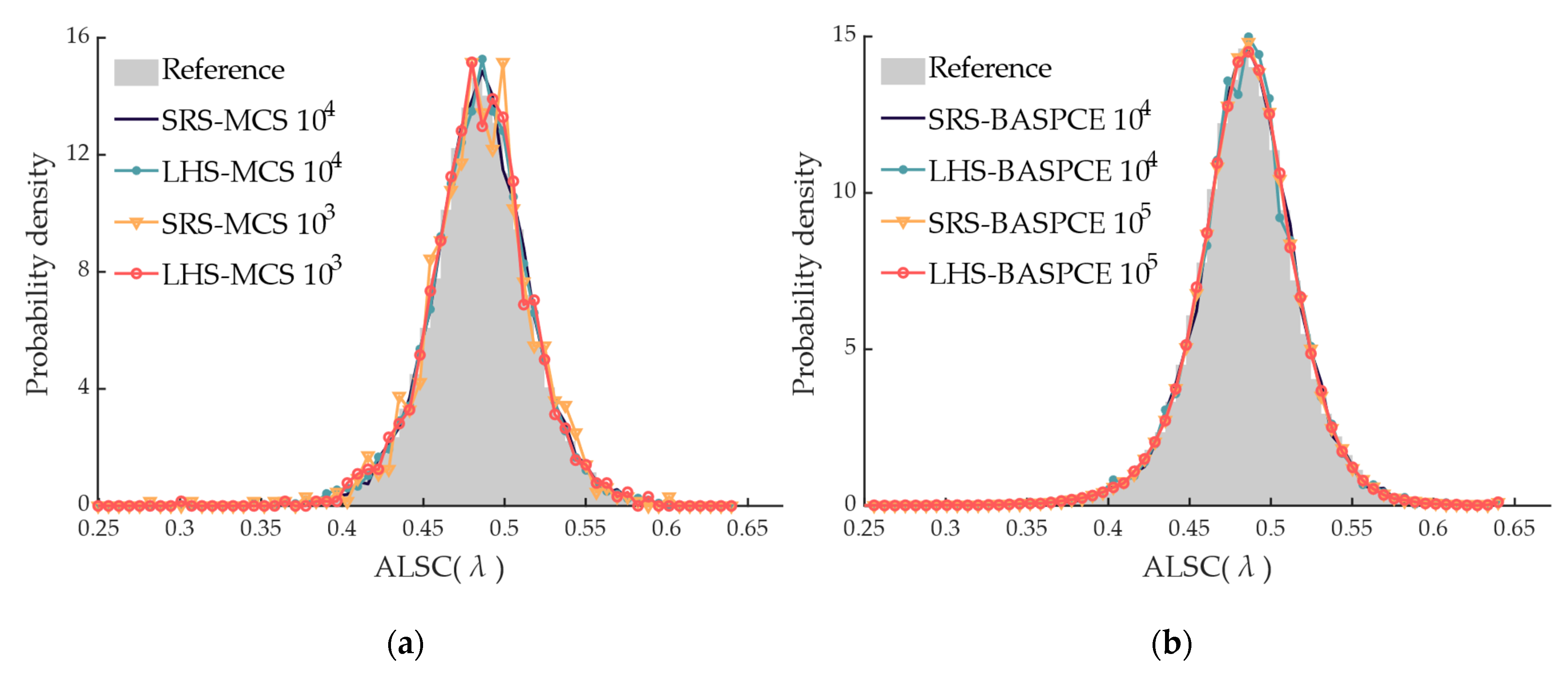
This paper systematically applies the BASPCE surrogate model to PRPF. Moreover, the GSA based on BASPCE is introduced in the ALSC evaluation to analyze the impact of power stations on the system’s LSC. The test results on the IEEE 39-bus system validate the feasibility and effectiveness of the proposed method. Detailed conclusions are drawn below.

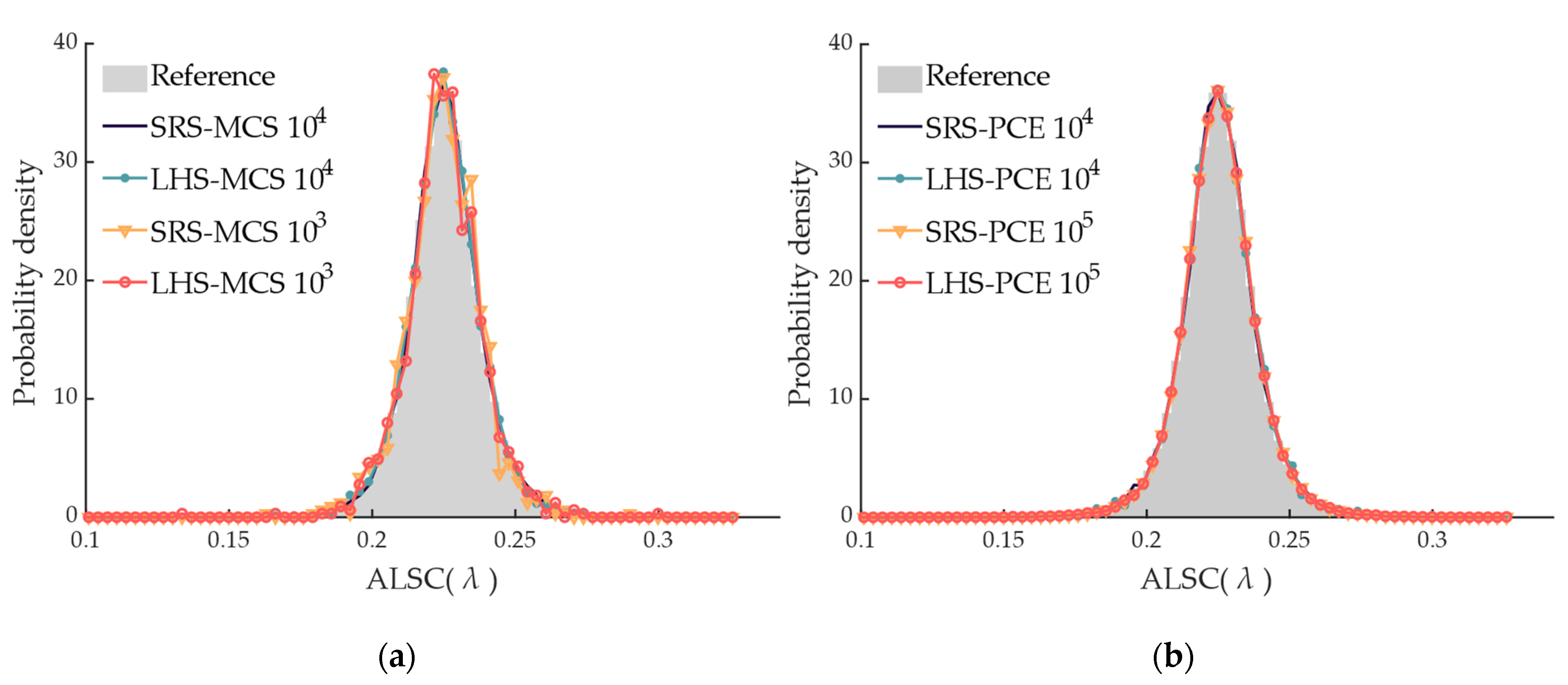
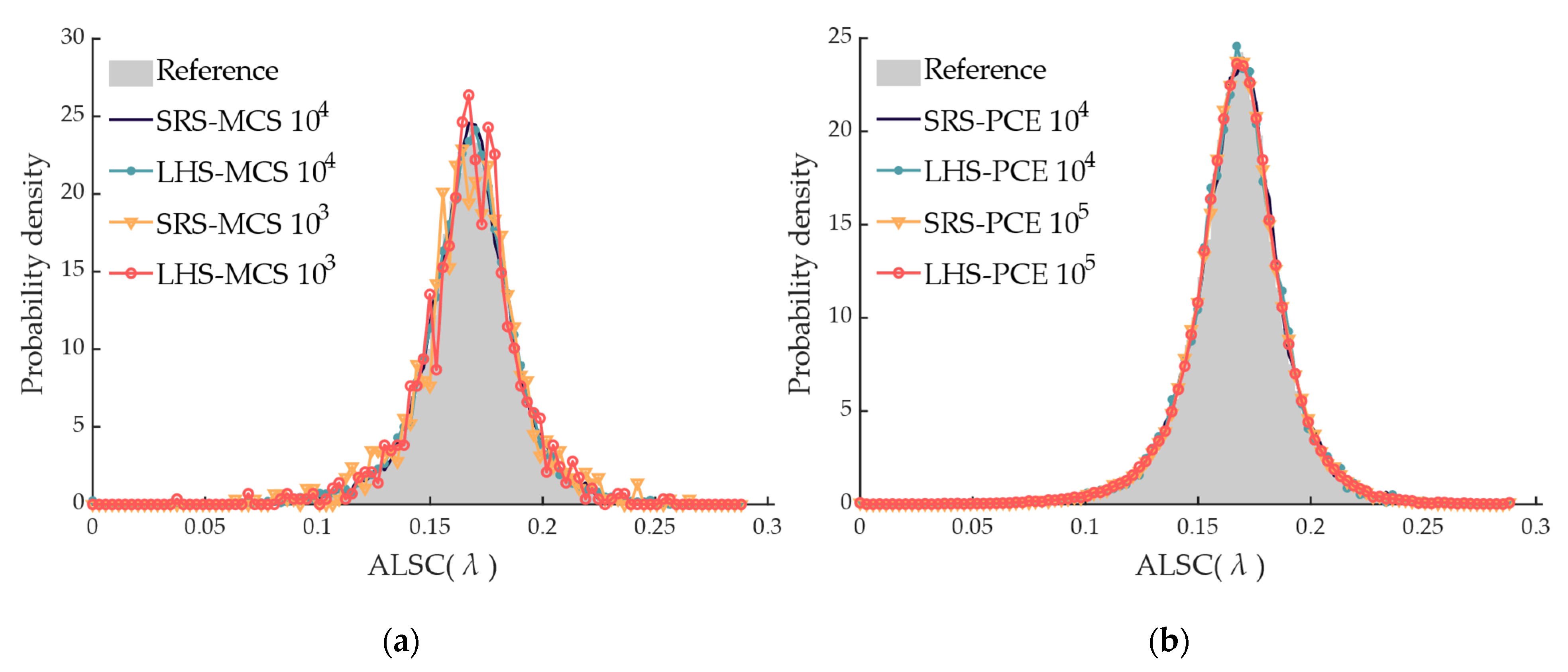
The BASPCE model can efficiently handle RPF with high accuracy and speed for probabilistic ALSC evaluation, as well as GSA based on RPF. More specifically, the distribution of ALSC obtained by the BASPCE is more than 97% similar to the reference. Furthermore, for ALSC evaluation, compared with the PRPF based on the original model, the PRPF based on BASPCE can reduce computation time by approximately tenfold without compromising accuracy. For GSA, since more rounds of MCS are required, the speed advantage of BASPCE becomes more pronounced, thus reducing computation time by over 30 times.

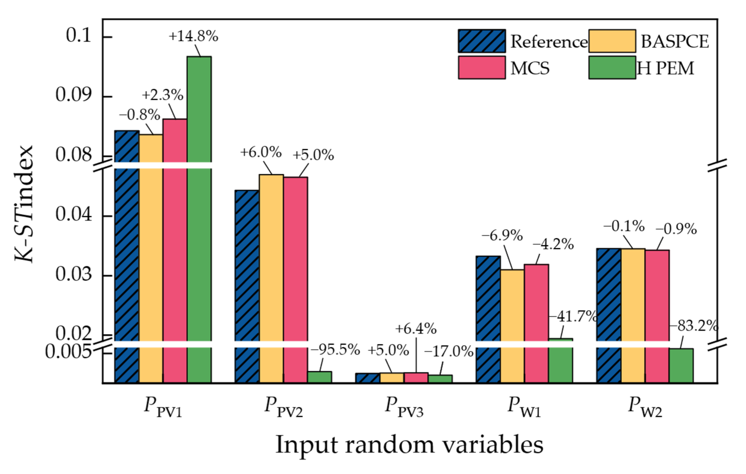
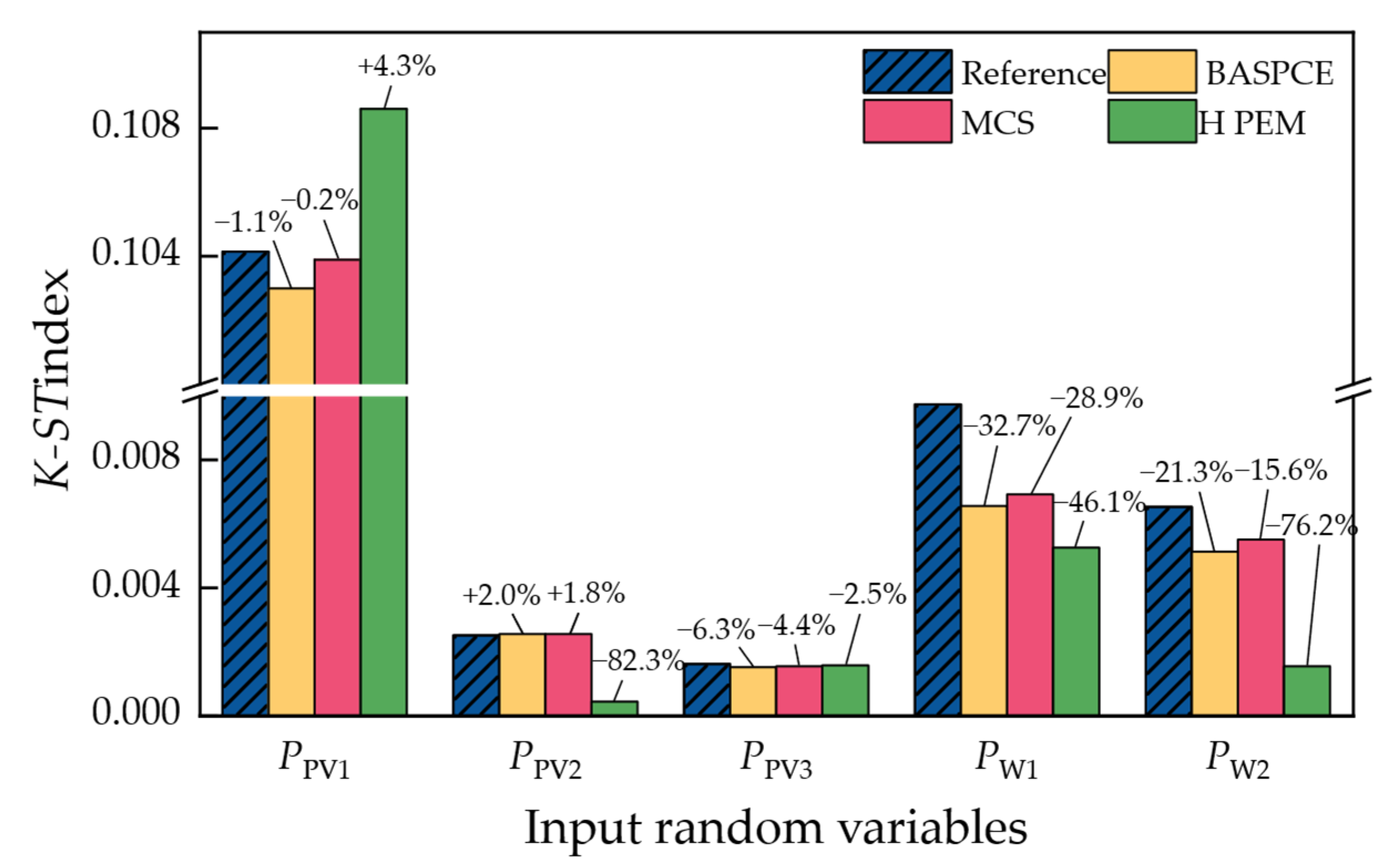
The results of the GSA can quantify the impact of uncertainties in renewable energy stations on LSC, and the ranking derived from GSA indices can assist in identifying the most critical renewable energy power stations.

The limitations of this study mainly lie in two aspects: first, the limitation of the RPF approach. RPF is a simple and effective approach for evaluating ALSC; however, its underlying assumption, a fixed load growth direction, may prevent it from identifying the maximum loading point. Therefore, developing more flexible methods that can account for varying load growth directions represents an important direction for future research.

Second, the limitation of the GSA indices: The GSA indices lack physical interpretability and only provide a relative ranking of influence. Therefore, a promising future direction is to develop a physically meaningful, station-level LSC index.

References

1. REN21. Renewables 2024 Global Status Report. REN21 Secretariat. 2024. Available online: https://www.lerenovaveis.org/contents/lerpublication/2024_abr_ren21_renewables-2024--global-status-report.pdf (accessed on 2 May 2025).
2. Ali, M.A.; Kamel, S.; Hassan, M.H.; Ahmed, E.M.; Alanazi, M. Optimal Power Flow Solution of Power Systems with Renewable Energy Sources Using White Sharks Algorithm. Sustainability 2022, 14, 6049. [Google Scholar] [CrossRef]
3. Rubino, L.; Rubino, G.; Esempio, R. Linear Programming-Based Power Management for a Multi-Feeder Ultra-Fast DC Charging Station. Energies 2023, 16, 1213. [Google Scholar] [CrossRef]
4. Zhang, S.; Cheng, H.; Zhang, L.; Bazargan, M.; Yao, L. Probabilistic Evaluation of Available Load Supply Capability for Distribution System. IEEE Trans. Power Syst. 2013, 28, 3215–3225. [Google Scholar] [CrossRef]
5. Xiao, J.; Lin, X.; Jiao, H.; Song, C.; Zhou, H.; Zu, G.; Zhou, C.; Wang, D. Model, Calculation, and Application of Available Supply Capability for Distribution Systems. Appl. Energy 2023, 348, 121489. [Google Scholar] [CrossRef]
6. Miu, K.N.; Chiang, H.-D. Electric Distribution System Load Capability: Problem Formulation, Solution Algorithm, and Numerical Results. IEEE Trans. Power Deliv. 2000, 15, 436–442. [Google Scholar]
7. Ou, Z.; Lou, Y.; Wang, J.; Li, Y.; Yang, K.; Peng, S.; Tang, J. The Effect of Power Flow Entropy on Available Load Supply Capacity under Stochastic Scenarios with Different Control Coefficients of UPFC. Sustainability 2023, 15, 6997. [Google Scholar] [CrossRef]
8. Shao, Q.; Liu, S.; Xie, Y.; Zhu, X.; Zhang, Y.; Wang, J.; Tang, J. Probabilistic Forecasting of Available Load Supply Capacity for Renewable-Energy-Based Power Systems. Appl. Sci. 2023, 13, 8860. [Google Scholar] [CrossRef]
9. Xu, Z.; Li, J.; Liu, H.; Ge, S.; Wang, B.; Wen, Z. Reliability-Based Power Supply Capability Evaluation of Power Distribution Networks Considering Interruptible Loads after Contingencies. Sustain. Energy Technol. Assess. 2024, 69, 103876. [Google Scholar] [CrossRef]
10. Xu, Z.; Liu, H.; Sun, H.; Ge, S.; Wang, C. Power Supply Capability Evaluation of Distribution Systems with Distributed Generations under Differentiated Reliability Constraints. Int. J. Electr. Power Energy Syst. 2022, 134, 107344. [Google Scholar] [CrossRef]
11. Xiao, J.; Li, F.; Gu, W.Z.; Wang, C.S.; Zhang, P. Total Supply Capability and Its Extended Indices for Distribution Systems: Definition, Model Calculation and Applications. IET Gener. Transm. Distrib. 2011, 5, 869–876. [Google Scholar] [CrossRef]
12. Ali, M.; Ali, M.H.; Gryazina, E.; Terzija, V. Calculating Multiple Loadability Points in the Power Flow Solution Space. Int. J. Electr. Power Energy Syst. 2023, 148, 108915. [Google Scholar] [CrossRef]
13. Kumar, S.; Ali, I.; Siddiqui, A.S. Energy Management in a Grid-Connected Microgrid Using Hybrid Golden Jackal Optimization and Gradient Descent Optimization and the Concept of Loadability. E-Prime—Adv. Electr. Eng. Electron. Energy 2024, 9, 100763. [Google Scholar] [CrossRef]
14. Kumar, A.; Deng, Y.; He, X.; Singh, A.R.; Kumar, P.; Bansal, R.; Bettayeb, M.; Ghenai, C.; Naidoo, R. Impact of Demand Side Management Approaches for the Enhancement of Voltage Stability Loadability and Customer Satisfaction Index. Appl. Energy 2023, 339, 120949. [Google Scholar] [CrossRef]
15. Pourbagher, R.; Derakhshandeh, S.Y.; Golshan, M.E.H. An Adaptive Multi-Step Levenberg-Marquardt Continuation Power Flow Method for Voltage Stability Assessment in the Ill-Conditioned Power Systems. Int. J. Electr. Power Energy Syst. 2022, 134, 107425. [Google Scholar] [CrossRef]
16. Yurtseven, K.; Ergun, H.; Van Hertem, D. Risk-Based Stochastic Optimal Power Flow for AC/DC Grids Using Polynomial Chaos Expansion. In Proceedings of the 2024 IEEE PES Innovative Smart Grid Technologies Europe (ISGT EUROPE), Srebreno, Croatia, 14–17 October 2024; pp. 1–5. [Google Scholar]
17. He, S.-Y.; Song, Y.; Cozza, A.; Xie, Y.-Z.; Wang, Z.-Y. A Fault Location Method Based on Polynomial Chaos Expansion for Non-Uniform Power Transmission Lines With Uncertainty Parameters. IEEE Trans. Electromagn. Compat. 2024, 66, 1665–1678. [Google Scholar] [CrossRef]
18. Rawal, K.; Ahmad, A. Stochastic Economic Dispatch with Advanced Polynomial Chaos Expansion. IFAC-Pap. 2024, 57, 155–160. [Google Scholar] [CrossRef]
19. De Mel, I.A.; Demis, P.; Dorneanu, B.; Klymenko, O.V.; Mechleri, E.D.; Arellano-Garcia, H. Global Sensitivity Analysis for Design and Operation of Distributed Energy Systems: A Two-Stage Approach. Sustain. Energy Technol. Assess. 2023, 56, 103064. [Google Scholar] [CrossRef]
20. Gao, Y.; Xu, X.; Yan, Z.; Wang, H.; Ping, J.; Yang, B.; Guan, X. Analytical Probabilistic Power Flow and Global Sensitivity Analysis of Distribution Systems Based on Gaussian Mixture Model of Input-Output Variables. IEEE Trans. Power Syst. 2024, 39, 5283–5296. [Google Scholar] [CrossRef]
21. Nikpour, A.; Nateghi, A.; Shafie-khah, M.; Catalão, J.P.S. Day-Ahead Optimal Bidding of Microgrids Considering Uncertainties of Price and Renewable Energy Resources. Energy 2021, 227, 120476. [Google Scholar] [CrossRef]
22. Parzen, E. On Estimation of a Probability Density Function and Mode. Ann. Math. Stat. 1962, 33, 1065–1076. [Google Scholar] [CrossRef]
23. Peng, S.; Tang, J.; Li, W. Probabilistic Power Flow for AC/VSC-MTDC Hybrid Grids Considering Rank Correlation Among Diverse Uncertainty Sources. IEEE Trans. Power Syst. 2017, 32, 4035–4044. [Google Scholar] [CrossRef]
24. Chen, Y.; Wen, J.; Cheng, S. Probabilistic Load Flow Method Based on Nataf Transformation and Latin Hypercube Sampling. IEEE Trans. Sustain. Energy 2013, 4, 294–301. [Google Scholar] [CrossRef]
25. Liu, P.-L.; Der Kiureghian, A. Multivariate Distribution Models with Prescribed Marginals and Covariances. Probabilistic Eng. Mech. 1986, 1, 105–112. [Google Scholar] [CrossRef]
26. Ni, F.; Nijhuis, M.; Nguyen, P.H.; Cobben, J.F.G. Variance-Based Global Sensitivity Analysis for Power Systems. IEEE Trans. Power Syst. 2018, 33, 1670–1682. [Google Scholar] [CrossRef]
27. Ernst, O.G.; Mugler, A.; Starkloff, H.-J.; Ullmann, E. On the Convergence of Generalized Polynomial Chaos Expansions. ESAIM: Math. Model. Numer. Anal. 2012, 46, 317–339. [Google Scholar] [CrossRef]
28. Marelli, S.; Lamas, C.; Konakli, K.; Mylonas, C.; Wiederkehr, P.; Sudret, B. UQLab User Manual—Sensitivity Analysis; Chair of Risk, Safety and Uncertainty Quantification; ETH Zurich: Zürich, Switzerland, 2024. [Google Scholar]
29. Tibshirani, R. The lasso method for variable selection in the Cox model. Stat. Med. 1997, 16, 385–395. [Google Scholar] [CrossRef]
30. Veras, M.B.A.; Mesquita, D.P.P.; Gomes, J.P.P.; Souza Junior, A.H.; Barreto, G.A. Forward Stagewise Regression on Incomplete Datasets. In Proceedings of the Advances in Computational Intelligence; Rojas, I., Joya, G., Catala, A., Eds.; Springer International Publishing: Cham, Switzerland, 2017; pp. 386–395. [Google Scholar]
31. Zhao, W.; Beach, T.H.; Rezgui, Y. Efficient Least Angle Regression for Identification of Linear-in-the-Parameters Models. Proc. R. Soc. A: Math. Phys. Eng. Sci. 2017, 473, 20160775. [Google Scholar] [CrossRef]
32. Blatman, G.; Sudret, B. Adaptive Sparse Polynomial Chaos Expansion Based on Least Angle Regression. J. Comput. Phys. 2011, 230, 2345–2367. [Google Scholar] [CrossRef]
33. Efron, B.; Stein, C. The Jackknife Estimate of Variance. Ann. Stat. 1981, 9, 586–596. [Google Scholar] [CrossRef]
34. Homma, T.; Saltelli, A. Importance Measures in Global Sensitivity Analysis of Nonlinear Models. Reliab. Eng. Syst. Saf. 1996, 52, 1–17. [Google Scholar] [CrossRef]
35. Kucherenko, S.; Tarantola, S.; Annoni, P. Estimation of Global Sensitivity Indices for Models with Dependent Variables. Comput. Phys. Commun. 2012, 183, 937–946. [Google Scholar] [CrossRef]
36. Janon, A.; Klein, T.; Lagnoux, A.; Nodet, M.; Prieur, C. Asymptotic Normality and Efficiency of Two Sobol Index Estimators. ESAIM: Probab. Stat. 2014, 18, 342–364. [Google Scholar] [CrossRef]
37. Zimmerman, R.D.; Murillo-Sánchez, C.E.; Thomas, R.J. MATPOWER: Steady-State Operations, Planning, and Analysis Tools for Power Systems Research and Education. IEEE Trans. Power Syst. 2011, 26, 12–19. [Google Scholar] [CrossRef]
38. Marelli, S.; Sudret, B. UQLab: A Framework for Uncertainty Quantification in Matlab. In Vulnerability, Uncertainty, and Risk; American Society of Civil Engineers: Reston, VA, USA, 2011; pp. 2554–2563. [Google Scholar]
39. Open Power System Data. Available online: http://Www.Open-Power-System-Data.Org/ (accessed on 2 May 2025).
40. Sheng, H.; Wang, X. Probabilistic Power Flow Calculation Using Non-Intrusive Low-Rank Approximation Method. IEEE Trans. Power Syst. 2019, 34, 3014–3025. [Google Scholar] [CrossRef]
41. Ni, F.; Nguyen, P.H.; Cobben, J.F.G. Basis-Adaptive Sparse Polynomial Chaos Expansion for Probabilistic Power Flow. IEEE Trans. Power Syst. 2017, 32, 694–704. [Google Scholar] [CrossRef]
42. Tang, J.; Ni, F.; Ponci, F.; Monti, A. Dimension-Adaptive Sparse Grid Interpolation for Uncertainty Quantification in Modern Power Systems: Probabilistic Power Flow. IEEE Trans. Power Syst. 2016, 31, 907–919. [Google Scholar] [CrossRef]
Figure 1. Schematic diagram of (a) DRPF and (b) PRPF.
Applsci 15 05169 g001
Figure 2. Schematic diagram of GSA for PRPF.
Applsci 15 05169 g002
Figure 3. Modified IEEE 39-bus system.
Applsci 15 05169 g003
Figure 4. Frequency histograms of ALSC using different methods in S1: (a) MCS-based methods and (b) BASPCE-based methods.
Applsci 15 05169 g004
Figure 5. Frequency histograms of ALSC using different methods in S2: (a) MCS-based methods and (b) BASPCE-based methods.
Applsci 15 05169 g005
Figure 6. Frequency histograms of ALSC using different methods in S3: (a) MCS-based methods and (b) BASPCE-based methods.
Applsci 15 05169 g006
Figure 7. K-ST index results calculated by different methods in S1.
Applsci 15 05169 g007
Figure 8. K-ST index results calculated by different methods in S2.
Applsci 15 05169 g008
Figure 9. K-ST index results calculated by different methods in S3.
Applsci 15 05169 g009