Research on the Self-Drilling Anchor Pull-Out Test Model and the Stability of an Anchored Slope

Abstract

We systematically investigated the anchorage performance of self-drilling anchor bolts in strongly weathered dolomite through integrated field pull-out tests and FLAC3D numerical modeling. The study incorporates symmetry principles in both experimental design and numerical simulations to ensure balanced force distribution and model simplification. Experimental data collected from a slope reinforcement project demonstrated that grouting parameters of 0.8 MPa pressure and 0.8 water–cement ratio achieved an interfacial bond strength of 0.147 MPa, surpassing the recommended value by 22.5%. A modified FLAC3D pile element, calibrated against RS6-01 anchor bolt test data, exhibited improved alignment with load–displacement curves, converging to 272 kN ultimate capacity at 26.1 mm displacement. Symmetrical anchor configurations in the numerical model reduced computational complexity while maintaining accuracy in stress distribution analysis. Through orthogonal experimental design, symmetry-driven parameter optimization identified a 7 m bolt length, 30° installation angle, and 2 m spacing as the most effective configuration. This solution increased the slope safety factor by 19.98% while reducing displacements by 46–62%. The symmetry in anchor spacing and angular alignment contributed to uniform stress redistribution, enhancing slope stability. The findings highlight the synergy between symmetry principles and geotechnical reinforcement strategies.

1. Introduction

Slope stability is a key issue in geotechnical engineering. In complex geological conditions or loose and fractured rock masses, traditional support technologies have been widely applied. However, in certain challenging conditions, such as fill soils and soft soils, issues such as borehole collapse, necking, insufficient anchor length, and poor grouting quality may occur [1,2]. These problems increase construction difficulty and may even compromise the safety of support structures and slope stability. To address these challenges, self-drilling anchor bolts have been increasingly adopted [3,4,5,6]. As an advanced anchoring technique, self-drilling anchor bolts are well-suited for complex geological conditions and challenging construction environments. They integrate drilling, grouting, and anchoring into a single process, offering simple construction and high efficiency. Due to these advantages, they are widely used in slope reinforcement, unstable rock mass stabilization, deep excavation support, and tunnel support [7].

Currently, there are numerous practical applications of hollow self-drilling anchor bolts in engineering. Yang Bo et al. verified, through the engineering practice at the Xigu Hydropower Station fault fracture zone slope, that the hollow self-drilling anchor bolts, with their simultaneous grouting characteristic through the hollow shaft, significantly improved the anchoring capacity of the surrounding rock and addressed the technical bottleneck of difficult hole formation. Shao Hongyan, based on case studies of hydropower projects, systematically analyzed the hole-formation efficiency and grouting effectiveness of hollow self-drilling anchor bolts in loose rock–soil formations, pointing out that their “drilling-grouting-anchoring” integrated process could significantly enhance the overall integrity of support structures. Similarly, Wu Hongfu, in an engineering project at a deep foundation pit in the mountainous area of Southern Anhui, verified that the construction process of self-drilling anchor bolts reduced the difficulty of hole formation, especially demonstrating greater advantages in gravelly soil layers. These achievements highlight that hollow self-drilling anchor bolts, when used to replace traditional soil nails, anchor cables (or bolts) for slope protection in complex geological conditions and can effectively resolve problems such as difficult hole formation, hole collapse, and slow drilling in such strata [8]. Furthermore, due to the elimination of casing for wall protection during construction, the use of hollow self-drilling anchor bolts greatly improves construction efficiency, shortening the project timeline while reducing overall construction costs [9,10]. However, research on the application of hollow self-drilling anchor technology for reinforcing steep loose rock slopes is relatively scarce. Widely used case studies are mostly concentrated in tunnel and foundation pit projects, and there is insufficient accumulation of case analyses in loose fractured slopes. Therefore, this paper primarily focuses on the anchoring performance of self-drilling anchor bolts, conducting numerical simulation analysis of anchorage through experimental and numerical methods. Additionally, the Pile element model is refined to make its simulation results closer to reality, and actual engineering examples are used to validate the supporting performance of self-drilling anchor bolts, providing theoretical guidance and technical support for similar engineering projects.

2. Experimental Analysis of the Key Performance of Hollow Self-Drilling Anchor Bolts

2.1. Experimental Design

This study is based on the hollow self-drilling anchor used in the project, which is R38S (produced by Hengnuo Anchoring Technology Co., LTD., Luoyang, China), as shown in Figure 1. The shaft is made of a thick-walled seamless steel pipe, with standard threaded connections along its entire length. The yield force of this type of anchor is 450 kN, the tensile force is 550 kN, the cross-sectional area is 631 mm², and the elongation is 8%. The drill bit is a full-steel ball-tooth drill bit, which is suitable for fractured formations, soft sandstone, limestone, gravel, and soft rock layers. The coupling sleeve has the same strength as the hollow shaft. The cement used is 42.5 grade composite silicate cement, and the grouting pressure is selected as 0.8 MPa with a water–cement ratio of 0.8, as per the design specifications.

The experimental design follows the requirements of the Technical Code for Ground Anchorages and Soil Nails (CECS 22:2015) and the Technical Code for Retaining and Protection of Building Excavations (JGJ 120–2012) [11]. The study focuses on verifying the anchoring mechanism and load-bearing characteristics of self-drilling anchor bolts in complex rock formations. The drilling process of self-drilling anchor bolts is illustrated in Figure 2.

During the experimental loading process, a QF-100-100 type hollow hydraulic jack (produced by Dezhou Huali Hydraulic Press Co., LTD., Dezhou, China) was used, as shown in Figure 3. Additionally, high-precision load sensors were installed throughout the system to ensure the accuracy of load measurements. To comprehensively monitor the displacement variations during the experiment, a total of four displacement meters were installed, with an accuracy of up to 0.01 mm. The design of the entire loading system followed the requirements outlined in Appendix D of the “Technical Code for Building Foundation Pit Support” (JGJ 120—2012), adopting a single-cycle incremental loading mode. In this mode, the load steps were set as 0.1 P, 0.5 P, 0.7 P, 0.8 P, and 0.9 P, progressing until the load corresponding to the estimated ultimate bond strength, denoted as P, was reached. The value of P was selected based on the engineering design documents. To ensure the stability and accuracy of the data, the duration of each load step was no less than 5 min, and the initial displacement was recorded prior to the start of loading. During the loading process, data were collected every 30 min to monitor displacement changes. The loading system continued to monitor the displacement until the convergence criteria were met, i.e., the displacement increment within two consecutive 1-h intervals did not exceed 0.1 mm. Only then would the next load step be applied, ensuring the rigor of the experiment and the reliability of the results.

Three failure criteria were established as the basis for determining failure and stopping the test:

(1)

Displacement divergence criterion: The displacement rate continuously increases at a given load level and exceeds 0.5 mm within one hour;

(2)

Load-bearing failure criterion: A significant turning point appears in the load–displacement curve, and the residual deformation reaches 80% of the peak displacement;

(3)

Rod body fracture criterion: The anchor bolt exhibits necking or fracture.

Once any of these criteria are met, the test is immediately terminated. The load level preceding failure is recorded as the ultimate uplift bearing capacity.

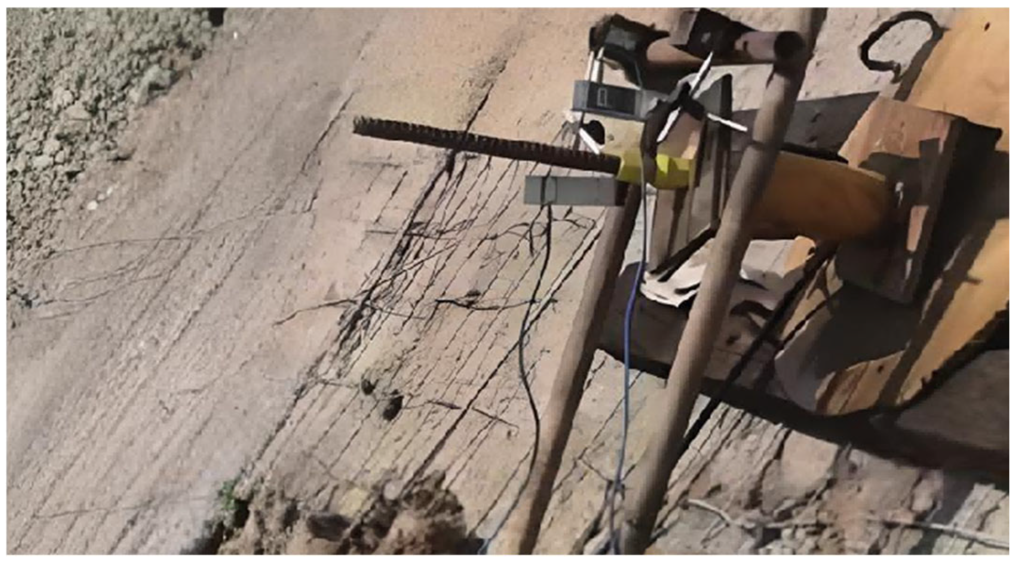
2.2. Overview of the Experimental Site Conditions

The experimental site is located in an open abandoned mine pit in the Jinpu New District of Dalian. Prolonged mining activities have resulted in multiple stages of artificial slopes with heights ranging from 30 to 50 m, presenting a stepped configuration. The slopes are primarily concave and straight, with some areas exhibiting irregular profiles. The slope angles vary between 35° and 60°. Due to geological and weathering effects, the rock mass is fragmented, with loose rock blocks accumulated and signs of slumping observed. The stratigraphy, from top to bottom, can be classified as follows: a gravelly sandy soil layer, a strongly weathered dolomite layer, and a weakly weathered dolomite layer. The site is unaffected by groundwater.

For the purpose of the experiment and to ensure the relative uniqueness of the variables, we selected a section of the slope with a thick exposure of the strongly weathered dolomite layer for the test. The slope inclination was artificially cut to 45° for the experiment.

The equipment layout for the field experiment is shown in Figure 4. The anchor bolts are arranged on the same slope surface. To minimize the influence of anchor bolt spacing on the test results, the anchor bolts are uniformly spaced at 3 m apart. Vertically, only two rows of anchor bolts are arranged, and the experiment is conducted using a method where the bolts are installed perpendicular to the slope surface.

2.3. Analysis of the Experimental Results

Through systematic uplift tests, a total of 24 sets of valid experimental data were obtained. When the anchor bolt models were RS4, RS6, RS8, and RS10, the measured values of their ultimate uplift capacity ranged from 178 to 208 kN, 257 to 383 kN, 289 to 367 kN, and 368 to 411 kN, respectively. The bond strength, which describes the bonding performance between the self-drilling anchor bolt anchorage body and the soil layer, is defined as the average bond stress at the interface between the anchorage body and the rock–soil mass within the anchoring section of the anchor bolt. It is calculated according to Equation (1).

$$\tau ={\displaystyle \frac{{{\displaystyle P}}_a}{\pi dl}}$$

(1)

In Equation (1), P_a represents the ultimate uplift strength of the anchor bolt (kN); l is the anchorage length (m); d is the diameter of the anchorage body (mm); and $\tau$ is the bond strength between the anchorage body and the surrounding soil (MPa).

According to

Table 1. Self-drilling anchor bolt test results.

Group	Number	Anchorage Length/m	Ultimate Uplift Capacity/kN	Bond Strength/MPa
RS4	RS4-01	3.66	178	0.155
	RS4-02	3.41	184	0.172
	RS4-03	3.89	197	0.161
	RS4-04	3.21	189	0.188
	RS4-05	3.93	208	0.169
	RS4-06	3.76	166	0.141
	Average	3.64	187	0.163
RS6	RS6-01	5.75	272	0.151
	RS6-02	5.53	257	0.148
	RS6-03	5.77	296	0.163
	RS6-04	5.84	269	0.147
	RS6-05	5.64	283	0.160
	RS6-06	5.57	269	0.154
	Average	5.68	274	0.154
RS8	RS8-01	7.12	289	0.129
	RS8-02	7.76	351	0.144
	RS8-03	7.66	333	0.138
	RS8-04	7.84	367	0.149
	RS8-05	7.54	347	0.147
	RS8-06	7.79	356	0.146
	Average	7.62	341	0.142
RS10	RS10-01	9.34	377	0.129
	RS10-02	9.68	389	0.128
	RS10-03	9.59	411	0.136
	RS10-04	9.83	368	0.119
	RS10-05	9.66	399	0.132
	RS10-06	9.79	403	0.131
	Average	9.65	391	0.129

The explanation of the meaning of the numbers in the table is the following (take RS4-01 as an example): RS stands for the self-drilling bolt model (taken from the bolt model RS38S in this test), the number 4 represents the length specification of the self-drilling bolt, and -01 represents the specific bolt number. The anchor solid diameter (hole size) of all bolts is uniformly 100 mm.

, the range and average values for each group of anchor bolts were obtained, from which the coefficient of variation for each group of anchor bolts was calculated as 22%, 14%, 23%, and 11%, respectively. The corresponding coefficient of the variation curve is shown in Figure 5a (blue curve). According to the criteria for data dispersion outlined in the “Technical Code for Foundation Pit Support” (JGJ120—2012) [11], which specifies that the range should not exceed 30% of the average value, the characteristic values of the ultimate uplift capacity for the four groups of anchor bolts can be taken as the average ultimate uplift capacity for each group, as recommended in the standard. These values are 187 kN, 274 kN, 341 kN, and 391 kN, respectively. Based on this, the relationship curve between anchorage length and average ultimate uplift capacity is plotted as the red curve in Figure 5a.

For the average bond strength of each group of anchor bolts, it is calculated using Equation (1) and the average ultimate uplift capacity values (187 kN, 274 kN, 341 kN, and 391 kN) determined according to the specifications mentioned earlier. After calculation, the average bond strengths for the four groups of anchor bolts are found to be 0.163 MPa, 0.142 MPa, 0.154 MPa, and 0.129 MPa, respectively. This bond strength value is derived from the average ultimate uplift capacity of each group of anchor bolts and directly reflects the relationship between the average ultimate uplift capacity and the average anchorage length for each group of anchor bolts. Although the standard does not provide explicit guidance on how to determine the bond strength for each group of anchor bolts, the results can be considered reliable. To ensure the rigor of the data, the coefficient of variation can also be introduced for verification. Generally, the coefficient of variation is used to compare the dispersion of different data sets. A smaller coefficient indicates lower dispersion and better data stability, while a larger coefficient suggests higher dispersion and poorer data stability. For continuous data, the normal range for the coefficient of variation is typically between 0% and 30%, while for discrete data, it generally ranges from 0% to 100%. Since the bond strength values for all anchor bolts are calculated using Equation (1), we consider the data to be relatively continuous. Consequently, the range for the coefficient of variation is also stricter in this case. The calculation of the coefficient of variation is illustrated using the data from the RS4 group as an example.

The average value (μ) for this set is calculated as follows:

$$\mu ={\displaystyle \frac{0.155+0.172+0.161+0.188+0.169+0.141}{6}}=0.163$$

(2)

The standard deviation (σ) is calculated as follows:

$$\sigma =\sqrt{{\displaystyle \frac{\begin{array}{l}(0.155-0.163{)}^2+(0.172-0.163{)}^2+(0.161-0.163{)}^2+\\ (0.188-0.163{)}^2+(0.169-0.163{)}^2+(0.141-0.163{)}^2\end{array}}{5}}}»0.016$$

(3)

From this, the coefficient of variation (C_v) can be obtained.

$$Cv={\displaystyle \frac{0.016}{0.163}}\times 100\%\approx 9.8\%$$

(4)

By following the same method, we can sequentially calculate the coefficient of variation for the experimental data of the four groups of anchor bolts. The coefficients of variation for RS4 to RS10 are 9.8%, 7.2%, 6.3%, and 4.7%, respectively. The coefficient of variation curve is shown in Figure 5b (blue curve). It can be seen that all the coefficient values are below 30%, which sufficiently demonstrates that the average bond strength values for each group of anchor bolts are reliable. Therefore, we can plot the red curve in Figure 5b using the average bond strength values of 0.163 MPa, 0.142 MPa, 0.154 MPa, and 0.129 MPa for the four groups of anchor bolts.

Taking the red curve in Figure 5a as the focus of the study, we can analyze the relationship between the ultimate uplift capacity of self-drilling anchor bolts and the anchorage length. Starting with the average anchorage length and ultimate uplift capacity of the first group of anchor bolts, we observe that as the average anchorage length increases from 3.64 m to 9.65 m, the ultimate uplift capacity increases from 187 kN to 391 kN. The ultimate uplift capacity of self-drilling anchor bolts increases nonlinearly with anchorage length. The curve shows that as the anchorage length increases, the growth rate of ultimate uplift capacity increases from 56% to 165%, while the growth rate of ultimate uplift capacity increases from 47% to 109%. This phenomenon can be explained by the mechanical mechanism at the anchorage interface: in loose and fractured strata, the shear resistance between the grouting material and the rock–soil mass is evenly distributed along the anchorage section, and the total uplift capacity is approximately the product of the anchorage length and the bond strength per unit length. This indicates that, within a specific range, increasing the anchorage length can effectively enhance the uplift performance of self-drilling anchor bolts.

As for bond strength, theoretical studies on the elastic shear transfer model [12,13,14,15] show that the bond strength distribution along the surface of the anchor bolt anchorage body is uneven. Simultaneously, by observing the blue curve in Figure 5b, we find that the coefficient of variation for longer anchorage sections is significantly lower than for shorter ones, suggesting that short anchorage sections are more affected by rock mass defects, whereas longer sections reduce randomness through spatial averaging effects. Moreover, as the anchorage length increases, the bond strength shows a decreasing trend, with the RS4 group exhibiting the highest bond strength and the RS10 group the lowest, indicating a significant negative correlation. This is consistent with the “effective anchorage length” theory, which suggests that simply increasing the anchorage length does not necessarily improve the load-bearing performance. Additionally, the non-uniformity of the spatial distribution of bond strength indicates that the average bond strength value obtained from traditional calculation formulas does not accurately reflect the actual stress field distribution. The shear stress at the interface of the anchorage section decays exponentially along the axis, with the maximum shear stress concentrated in the proximal region. As the anchorage length increases, the proportion of the effective load-bearing section decreases. Beyond the critical length, the distal section does not participate in load transfer, leading to an overall reduction in bond strength, particularly noticeable in soft rocks and fractured strata.

We calculated the increment in ultimate uplift capacity and the decrease in average bond strength between adjacent anchor bolt groups, from which we can plot the ultimate uplift capacity increment curve (blue curve) and the decrease in average bond strength curve (red curve).

From Figure 6, we can observe that as the anchorage length increases, particularly in the range of 6 to 10 m, the increment in the ultimate uplift capacity of the self-drilling anchor bolts shows a significant decrease, dropping from 46.5% to 14.7%. Correspondingly, the decrease in the average bond strength gradually increases from 5.9% to 9.3%. Although a comparison of the magnitude changes reveals that between anchorage lengths of 5.68 m and 9.65 m, the increase in the decrease in average bond strength is not significant, and it follows a nearly linear relationship with a relatively mild curve, the increment in the ultimate uplift capacity shows a diminishing trend with increasing anchorage length. For the 10-m group (RS10), the increment has rapidly decreased to 14.7%. This suggests that, from an efficiency perspective, the anchorage length of self-drilling anchor bolts in this type of soil layer should not exceed 8 m.

3. Self-Drilling Anchor Bolt Anchorage Mechanism Simulation Study

3.1. Selection of the Numerical Simulation Model

When simulating anchor bolts in FLAC3D 6.0 software, built-in anchor bolt units or pile units are generally used as linear structural elements. These units can effectively represent the structural response of a mechanical system composed of solid continuous media and supporting structures. It is worth noting that the pile unit can simulate the anchor bolt support characteristics by activating the “pile property rock bolt on” command. In this mode, the pile unit retains mechanical characteristics similar to those of the anchor bolt unit while also possessing unique functions: it can quantify the distribution of surrounding restraint stresses in the support body, characterize the strain softening properties between the anchor bolt and surrounding rock, and establish failure criteria for anchor bolt uplift and rupture. The pile unit in the software uses a one-dimensional linear model to simulate the axial mechanical behavior of the anchor bolt. Additionally, it employs a tangential and normal coupled spring mechanism to accurately reflect the bond and friction characteristics at the anchor bolt–anchorage–soil interface. The numerical simulation process for the anchor bolt’s action mechanism in the software is shown in Figure 7.

According to the software user manual, the shear force at the interface between the pile unit and the solid mesh unit is a function of the interface bond strength and the interface frictional force. Equation (5) describes the maximum shear force for a unit length pile, which can be used to estimate the relevant parameters. Additionally, FLAC3D software allows the definition of shear coupling springs through a table function programming, which models the softening of the cohesion and friction angle of the shear coupling springs. This, in turn, adjusts the effective lateral confinement stress defined by the parameters.

$${\displaystyle \frac{F_{T\max }}{L}}=s{c}_h+{\tau }_{\mathrm{u}}\times \tan (s{c}_f)\times perimeter$$

(5)

In the formula:

F_Tmax is the maximum shear force of the anchor body, N;

sc_h is the cohesion per unit length of the shear coupling spring, N/m;

τ_u is the shear strength of the anchor body, Pa;

sc_f is the friction angle within the shear coupling spring, in °;

perimeter is the outer perimeter length of the anchor body, m.

3.2. Model and Parameter Selection

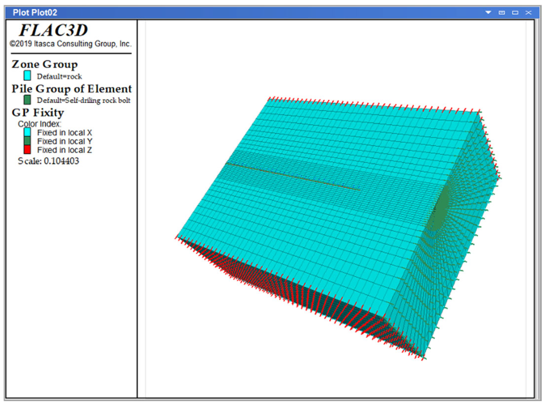
3.2.1. Numerical Model Construction

In FLAC3D software, the pile element nodes have six degrees of freedom, while the anchor bolt element only has axial degrees of freedom. Therefore, the pile element can accurately simulate the frictional interaction between the pile and the mesh elements and can be applied to simulate the complex mechanical behavior of anchor bolt pullout. Thus, in this study, the pile element is used to simulate the self-drilling anchor bolt uplift test. The size of the soil area for simulation is set to 3 × 3 × 8 m, and the Mohr–Coulomb constitutive model is used for simulation. It should be noted that, in reality, the soil is not a strict homogeneous body, and there may be local fractures and joints. However, to simplify the simulation, we assume that the soil is isotropic.

We take the direction from the bottom to the top of the soil layer as the positive Y-axis direction, and the geometric center of the model as the coordinate origin. The soil is modeled using the radial-cylinder command, and the discretization is achieved by changing the segments and ratio parameters. The mesh density decreases outward, ensuring that the mesh around the anchor bolt research object is the densest, while the mesh in the edge soil can be relatively sparse due to its relatively weak influence. Finally, the reflect command is used to mirror the soil to complete the construction of the overall soil area model. In FLAC3D, the built-in pile element is used to simulate the self-drilling anchor bolt, and it is automatically bound to the adjacent soil elements. The anchor bolt parameters are based on the RS6-01 anchor bolt, with a length of 6 m, a diameter of 0.038 m, an anchor solid diameter of 0.1 m, an outer circle circumference of 0.3142 m, and a length of 5.75 m. The soil area of the model generates a total of 36,480 zone element mesh nodes and 37,800 zone mesh elements. The pile element is divided into 23 elements using the segments command to ensure independent nodes. For the establishment of the boundary conditions of the computational model, the fix velocity command is used to apply displacement and velocity constraints in the xyz directions at the bottom of the model soil and in the normal direction around the soil. The top surface of the soil is set as a free surface without constraints. The model and the arrangement of the model mesh division and boundary constraints are shown in Figure 8.

3.2.2. Selection of Calculation Parameters

The formulas for calculating the grout cohesion and grout stiffness, which are essential for the numerical simulation, are as follows. These are defined as the tensile force per unit length applied to the anchor bolt and the slope of the force–displacement curve per unit length of the anchor bolt, respectively:

$${{\displaystyle C}}_g={\displaystyle \frac{{{\displaystyle P}}_a}{L}}=\pi dr$$

(6)

$${{\displaystyle K}}_g={\displaystyle \frac{{{\displaystyle C}}_g}{u}}$$

(7)

C_g is the grout cohesion, in N/m;

K_g is the grout stiffness, in N/m²;

P_a is the maximum uplift force applied to the anchor bolt during uplift, in N;

L is the anchorage length, in meters;

D is the anchor bolt diameter, in meters;

τ is the bond strength between the anchor bolt and the grout, in Pa;

u is the displacement length during the uplift of the anchor bolt, in meters.

The parameters of the anchorage system can be calculated using Equations (6) and (7), where the anchorage body diameter is D = 100 mm, the anchorage length of the self-drilling anchor bolt is L = 5.75 m, and the displacement length during anchor bolt uplift is u = 26.1 mm. The parameter values for the uplift simulation model of the self-drilling anchor bolt are shown in

Table 2. Parameters for the anchor system and geotechnical materials.

Anchor System Material Parameters				Soil Material Parameters
unit weight/(kg/m³)	7.18	Grouting cohesion/N·m−1	4.73 × 104	unit weight/kN·m−3	20.7
Elastic modulus/Pa	2.1 × 1011	Shear coupling spring internal friction angle/°	23	Bulk modulus/MPa	1915
Poisson’s ratio	0.3	Y-axis moment of inertia/m−4	3.21 × 10−9	shear modulus/MPa	885
Cross sectional area of the rod body/mm²	632	Z-axis moment of inertia/m−4	3.21 × 10−9	Poisson’s ratio	0.3
Anchor body circumference/m	0.314	polar moment of inertia/m−4	6.43 × 10−9	cohesion/Pa	24.2
Shear coupling spring stiffness/N·m−2	1.818 × 106	yield strength/kN	272	internal friction angle/°	26

.

3.3. Uplift Simulation of Self-Drilling Anchor Bolts

3.3.1. Initial Stress Equilibrium

Before simulating the uplift test, an initial equilibrium process must be carried out on the geotechnical strip to establish the initial stress and displacement fields and to eliminate any node displacements and node velocities generated during this process. Figure 9 and Figure 10, respectively, show the initial stress contour and the initial displacement contour.

3.3.2. Correction Method for Pile Elements

This study modifies the pile element based on a residual strength (strain-softening) model, which includes a three-segment post-peak softening model. The first segment represents the elastic deformation stage before the peak, the second segment represents the stress reduction stage after the peak, and the third segment represents the phase where the stress remains at a lower residual strength after a sharp drop, as shown in Figure 11. It should be noted that, from a practical engineering perspective, the interface stress model is not an absolute linear model but rather resembles the model shown in Figure 12. However, if we wish to extract data from all points, the only approach currently available is to consider it from a theoretical derivation standpoint, which also becomes the target direction for our next step of work.

Based on the above, the following effect can be achieved in FLAC3D. It is important to emphasize that in the modified pile element model, the implementation approach involves reading key points from the experiment, converting them into the anchorage interface unit cohesion (C_g) using Equation (6), and finally rewriting the linear curve in the Fish language. This curve is then assigned to the pile structural element using the table function to represent the characteristics of the anchorage interface. The method is universal for anchor bolts under different parameters, but the values assigned may differ. Therefore, this study focuses on simulating and analyzing the RS6-01 anchor bolt. As a result, we obtain the two curve models for the modified pile element shown in Figure 13. These curves describe the variation in unit bond strength at the interface and the ultimate uplift capacity of the anchor bolt. All subsequent simulation result analyses are based on this model.

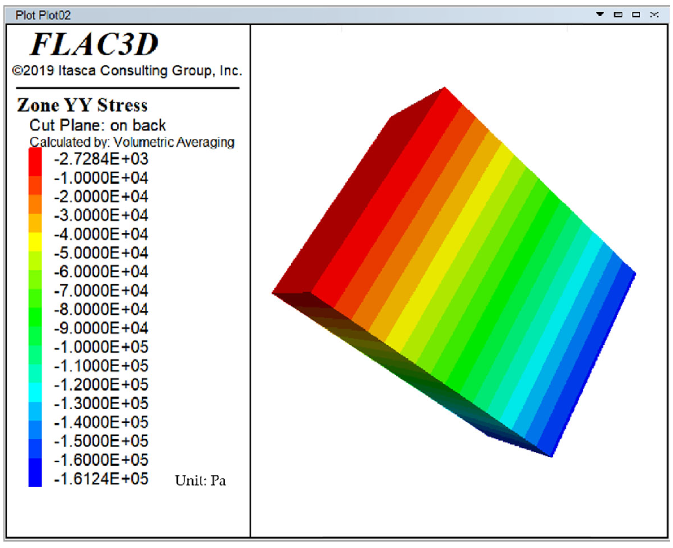
3.4. Analysis of Numerical Simulation Results

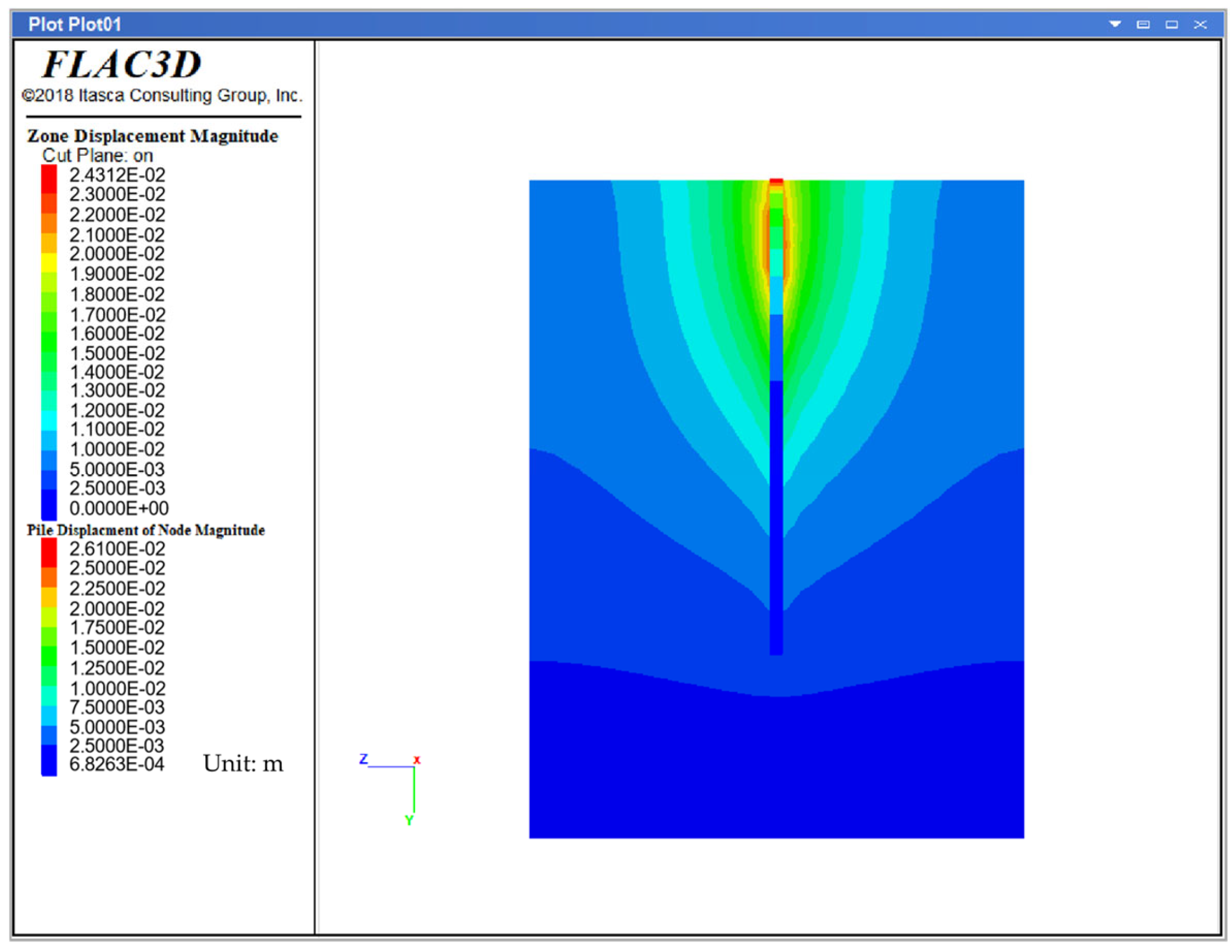
3.4.1. Displacement Result Analysis

Based on the initial stress field analysis, the “initial” command was used to set the velocity and displacement of all nodes in the model to zero along the XYZ axes, and then the uplift test of the self-drilling anchor bolt was simulated. A constant velocity boundary of 1 × 10⁻⁶ m/step along the Y-axis was applied to the exposed end nodes using the “initial” command, simulating the uplift process until the displacement reaches 26.1 mm, at which point the anchorage system fails. In the simulation, the displacement at the exposed end is the product of the constant velocity and the calculation step number. Meanwhile, the variations in axial force and shear stress during the uplift process were observed. Using the Fish language, the uplift load of the modified pile element at the corresponding displacement values was output based on the displacement values corresponding to each experimental data point. Under the condition of keeping the model soil parameters unchanged, the original unmodified pile element was also used to simulate the self-drilling anchor bolt. The resulting curve is shown in Figure 14.

By observing the three data curves in Figure 14, it is clear that the magenta curve for the unmodified pile element does not match the experimental curve at all, whereas the blue curve for the modified pile element shows a high degree of agreement with the experimental numerical curve. However, due to the ideal conditions under which the numerical model is established, the modified pile element shows a slight lag in the elastic phase. At the same displacement, the numerical values are slightly lower than the experimental values by 6–9 kN. Additionally, the modified pile element enters the plastic phase later than observed in the experiment. In the experiment, when the displacement reaches 8 mm and the ultimate uplift capacity is around 195 kN, the anchor bolt enters the plastic deformation phase. In contrast, the modified pile element enters the plastic phase at 9 mm and around 210 kN. Once in the plastic phase, due to the near-ideal simulation conditions, the simulation curve for the modified pile element deviates slightly from the experimental values, with the corrected value being about 1% to 6% higher than the experimental data. When the anchor bolt begins to enter the partial failure stage around 20 mm of displacement and continues until 26.1 mm, when the ultimate uplift capacity reaches 272 kN and the anchor bolt enters the complete failure state, the curve for the modified pile element closely overlaps with the experimental curve. Therefore, it can be concluded that the modified pile element provides a good representation of the actual behavior in the model.

The displacement contour plot at the ultimate uplift capacity of the self-drilling anchor can be seen in Figure 15. From Figure 15, it is evident that during the uplift process, a significant collaborative deformation phenomenon occurs between the pile unit anchor and the surrounding soil. Specifically, as the depth along the anchor centerline increases, the displacement of the soil also gradually increases. Moreover, the soil around the pile unit anchor exhibits a conical increase trend, resulting in an overall inverted conical shape in the displacement contour plot. This shape closely resembles the actual failure mode.

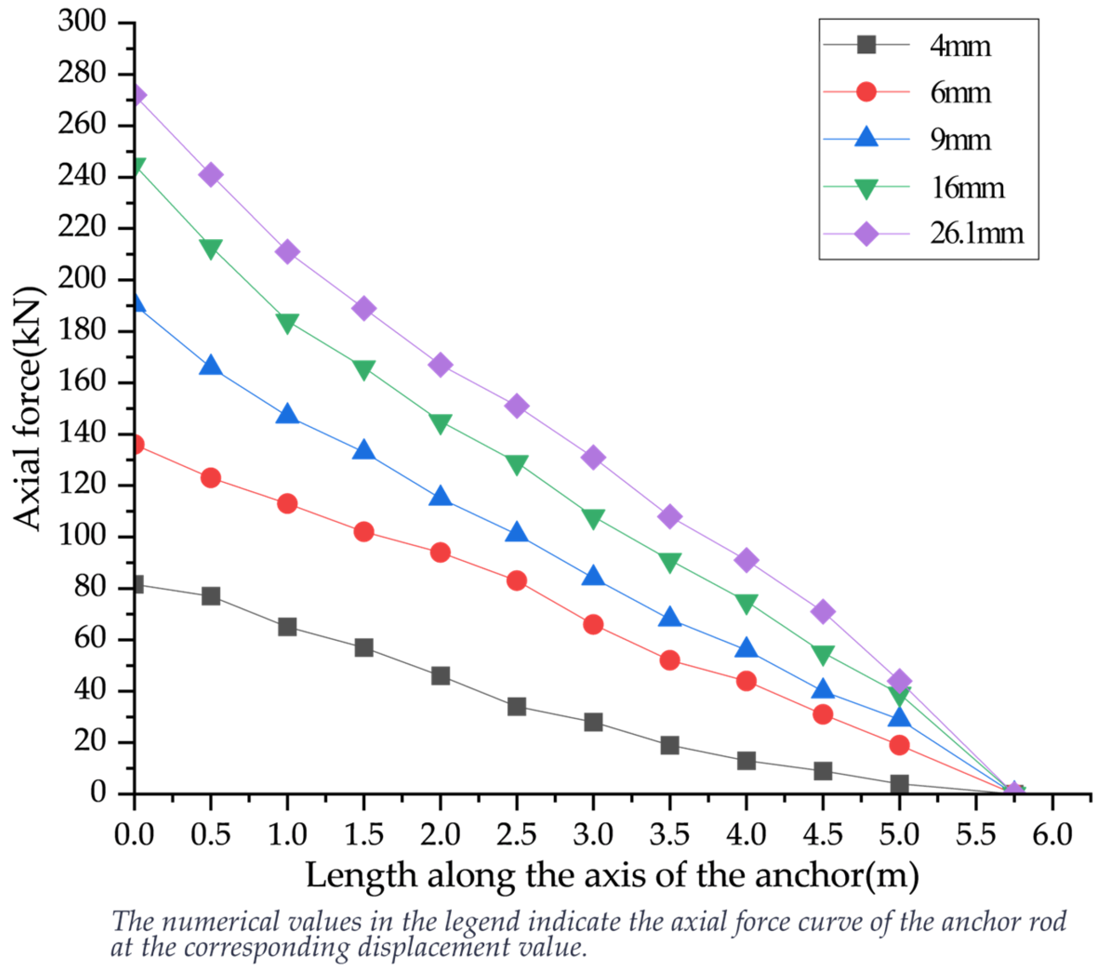
3.4.2. Anchor Axial Force Analysis

The curve in Figure 16 reflects the variation in axial force along the self-drilling anchor axis under different anchor displacements. As shown in Figure 16, the axial stress of the self-drilling anchor decreases gradually with increasing anchorage depth, with the limit of axial stress occurring at approximately 5.75 m. It can also be observed that when the applied load is less than 190 kN, the axial force curve of the self-drilling anchor follows a convex shape, indicating that the load decreases more gradually at the front end of the anchor, while the decay is more significant at the rear end. When the pullout load exceeds 190 kN, the curve begins to show a concave shape, with a significant reduction occurring in the 0–2 m range. This behavior is more intuitively reflected in the axial force contour plots of the anchor at different displacements in Figure 17. In these plots, the axial force is predominantly largest near the load application end and gradually decreases toward the far end along the anchor axis, following the same distribution pattern as the curve. Additionally, the axial force curve demonstrates that as the pullout load increases, relative slippage occurs, and the interface between the anchor and the surrounding soil will primarily rely on residual bond strength and friction to maintain its resistance. This results in the axial force shifting rapidly toward the deeper part of the anchor body, leading to a relatively rapid decay of the axial force.

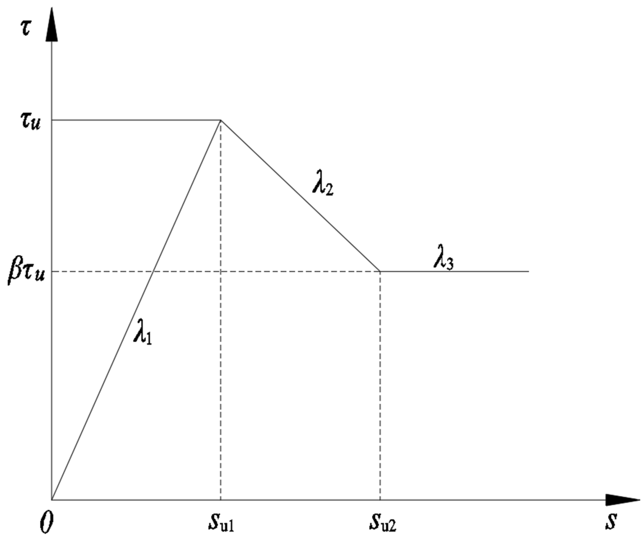
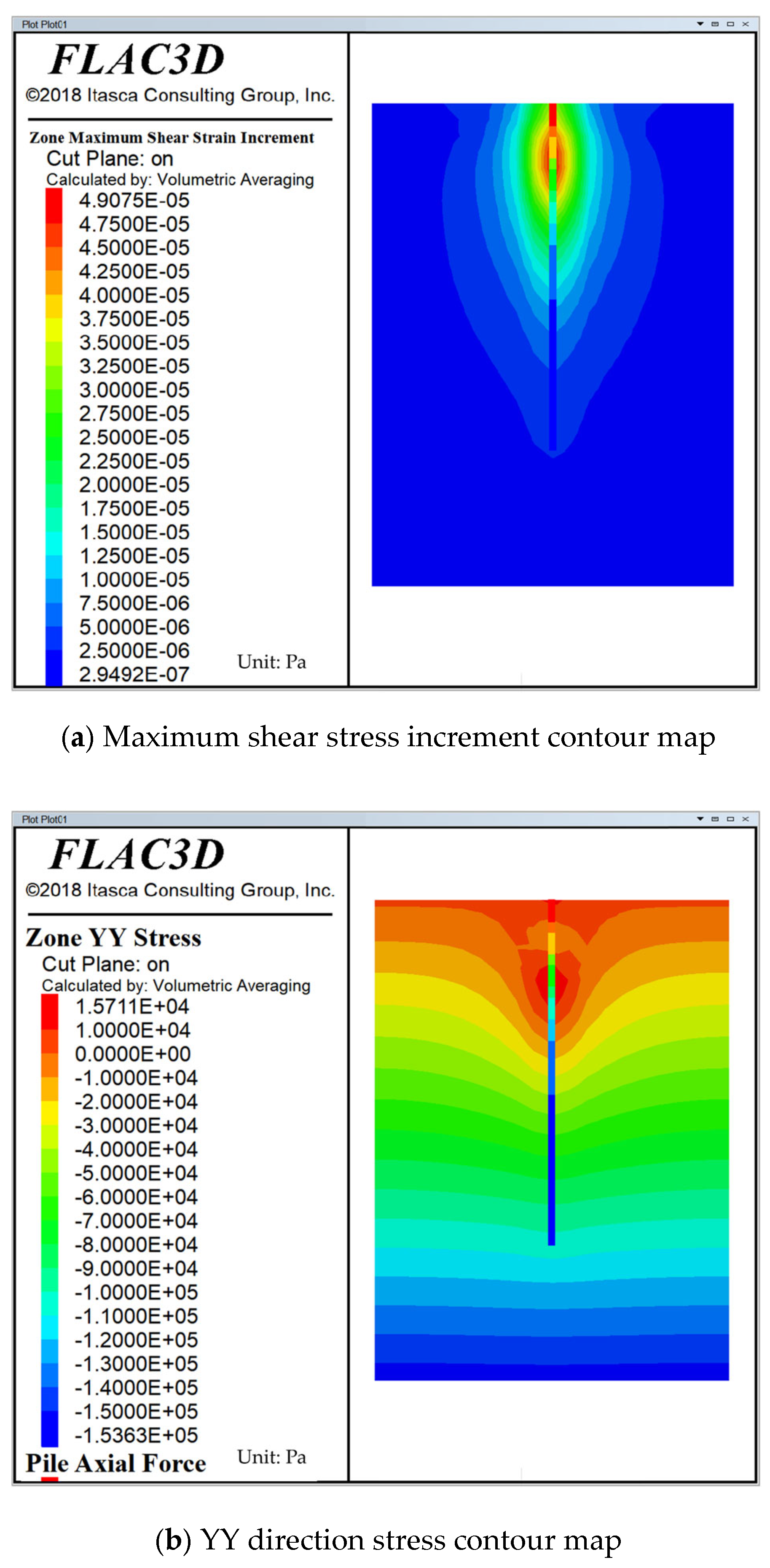
3.4.3. Interface Shear Stress Result Analysis

Figure 18 illustrates the stress distribution curve along the anchor–soil interface, extending along the length of the anchor rod. These values cannot be directly read but must be back-calculated using Equation (6) from earlier in the text. The curve demonstrates that the interface stress (or bond strength) is not uniformly distributed and, as the load increases, the maximum bond strength shifts deeper into the soil. Additionally, the maximum bond strength gradually increases until it reaches its peak value, which, for the RS6-01 anchor parameters, is 0.151 MPa. After the peak, the stress also increases with increasing displacement or ultimate pullout capacity of the anchor. As seen from the figure, the pre-peak stress reaches a plateau, with the displacement exceeding 16 mm before becoming nearly constant. This linear segment indicates that the bond effect at the front of the anchor has failed, and the stress present at the interface is now residual stress.

By analyzing the interface stress, it can be concluded that the equivalent bond strength parameter used in traditional homogenization theories cannot accurately describe the actual stress distribution along the anchor–soil interface. Systematic analysis of the pullout test results shows that the interface bond strength decays exponentially along the axial direction of the anchor. As the anchorage length increases, the proportion of the effective bearing section decreases non-linearly. Once the critical anchorage length is exceeded, the distal section becomes ineffective in transmitting stress, and the discontinuity at the interface leads to a reduction in the overall bond strength parameter.

Since pile elements are used for simulation, it is not possible to directly observe the interface stress between the anchor and the surrounding soil. However, we can indirectly derive the stress variation trend at the interface by analyzing the soil’s shear stress increments and the stress in the YY direction. Figure 19 presents the maximum shear stress increment and the stress in the YY direction for the surrounding soil when the self-drilling anchor reaches its ultimate pullout capacity. Upon examining the contour maps, it is evident that the peak soil stress and maximum shear stress increment are mainly concentrated at the front end of the anchor. This result aligns with the curve comparison, confirming its accuracy. Additionally, it can be observed in the contour map that the soil stress in the area of maximum axial force at the anchor’s front end is not high. This is because, when the ultimate pullout capacity is reached, the front end of the anchor undergoes failure and slip. Consequently, in this segment, it is assumed that only residual stress and the stress transmitted from the rear soil influence the region.

4. Self-Drilling Anchor Grouting Slope Simulation Analysis

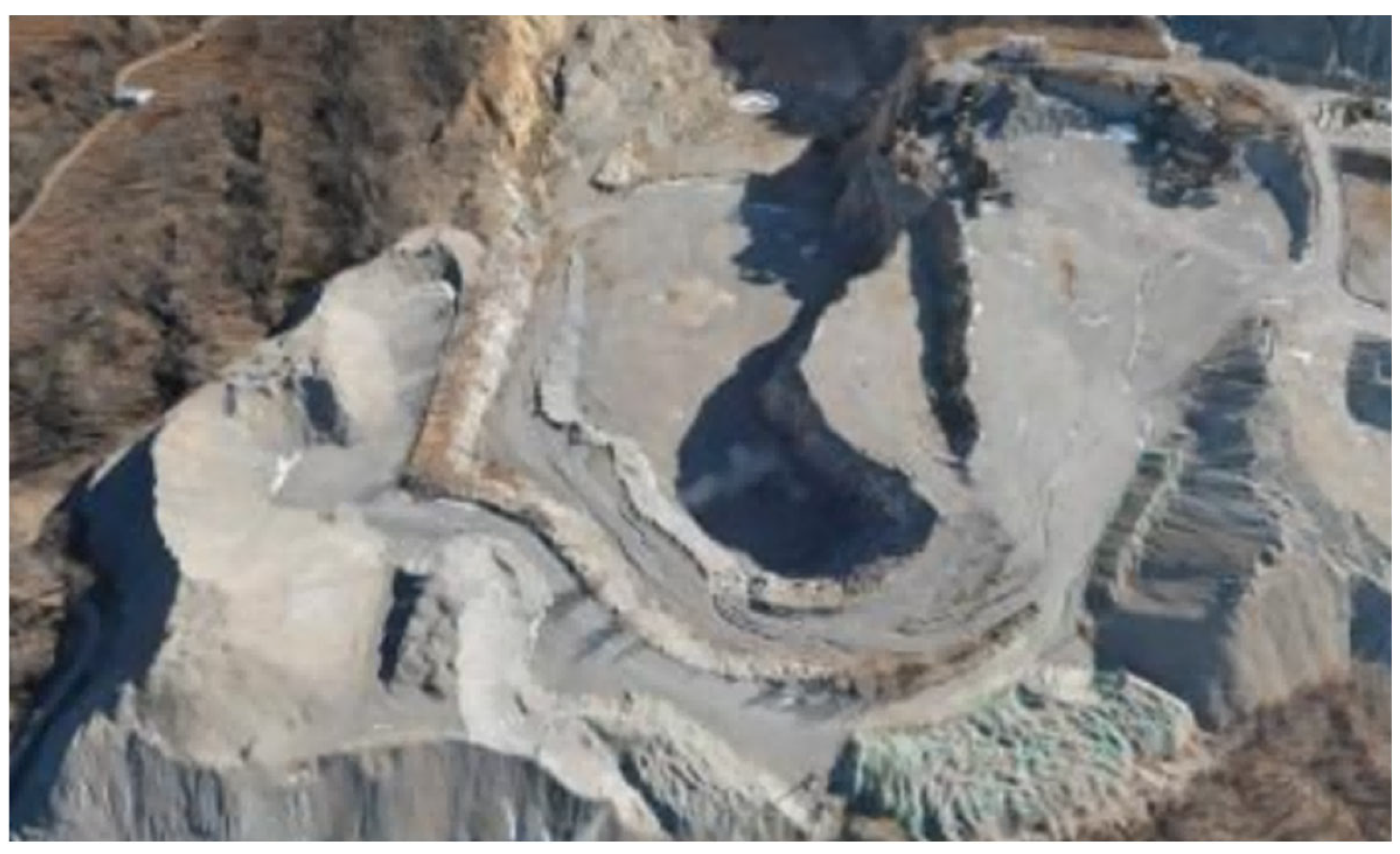
4.1. Project Overview

This section of the model is based on the reconstruction project of an abandoned open-pit mine in the Jinpu New Area of Dalian City, as shown in Figure 20. The mining area was originally a hilly landscape, with an elevation ranging from 80 to 180 m and a relative height difference of 50 to 100 m. The area slopes from north to south with a natural gradient of 15 to 25°, locally reaching over 30°. Long-term mining has resulted in multi-level artificial slopes with heights ranging from 30 to 50 m, forming a stepped structure. The slopes are predominantly concave and linear, with some irregular cross-sections. The slope angles range from 35° to 60°, and the rock mass is weathered and fractured due to geological and weathering processes, with loose rock fragments accumulating and evidence of sliding and collapse. The stratigraphy includes a surface layer of gravelly sandy soil, 4 to 8 m thick, with loose structure and high permeability; a highly weathered dolomitic limestone layer, 10 to 15 m thick, with a fragmented structure and well-developed joints and fractures; and a weakly weathered dolomitic limestone layer, with a relatively intact structure but with gently inclined structural planes.

4.2. Slope Model Optimization

4.2.1. Numerical Model and Calculation Parameters

A slope reduction scheme was implemented for the original slope to reduce the slope load. The slope reduction design is shown in Figure 21. The design adopts a three-tier slope reduction with a slope ratio of 1:1 and a 2-m-wide platform. Based on the engineering geological profile, the original slope and its reduction were simplified using AutoCAD2020 software, and the schematic diagram was imported into FLAC3D software. The Extrusion module was employed for the preprocessing of the slope model grid. The model’s coordinate system was defined such that the direction of horizontal sliding of the slope’s geotechnical body was the negative x-axis, and the z-axis positive direction was from the bottom to the top of the slope. The coordinate origin was located at the outer side of the slope’s toe. The model grid was divided at 1-m intervals. Boundary constraints were applied to the slope using the fix velocity command, with normal constraints applied to all surfaces of the slope except for the slope face, top, and bottom. The stratigraphy, boundary conditions, and model grid divisions are illustrated in Figure 22a for the original slope calculation model and Figure 22b for the slope calculation model after reduction.

In FLAC3D software, the soil is modeled by the Mohr–Coulomb constitutive model, which usually uses the bulk modulus (K) and shear modulus (G) instead of Young’s modulus (E) and Poisson’s ratio (ν). The bulk modulus (K) represents the material’s ability to resist volumetric changes, while the shear modulus (G) represents the material’s ability to resist shear strain. Since K and G provide a more accurate description of material deformation, E and ν need to be converted into K and G for numerical simulation calculations. The conversion formulas are as follows:

$$K={\displaystyle \frac{E}{3\left(1-2\nu \right)}}$$

(8)

$$G={\displaystyle \frac{E}{2\left(1+\nu \right)}}$$

(9)

In the equation:

E is the elastic modulus of the geotechnical material,

v is the Poisson’s ratio of the soil.

The model parameters are detailed in

Table 3. Soil parameters of the numerical model.

Type	Young’s Modulus (Pa)	Density (kg/m³)	Cohesion (Pa)	Internal Friction Angle (°)	Poisson’s Ratio	Bulk Modulus (Pa)	Shear Modulus (Pa)
Sandy soil with gravel	3.60 × 108	1.97	1.80 × 104	19	0.33	4.08 × 107	2.39 × 108
Strongly weathered dolomite	2.20 × 109	2.09	2.44 × 104	26	0.3	2.93 × 108	1.43 × 109
Weakly weathered dolomite	8.60 × 109	2.22	4.60 × 104	39	0.2	1.72 × 109	5.16 × 109

and

Table 4. Anchor parameters of the numerical model.

Anchor Bolt Type	Young’s Modulus (MPa)	Grouting Cohesion (N/m)	Grouting Stiffness Value (Pa)	Grouting Friction Angle	Drilling Diameter (mm)
Self-drilling anchor bolt	2.0 × 1011	48.2 × 103	11.4 × 106	30	100

.

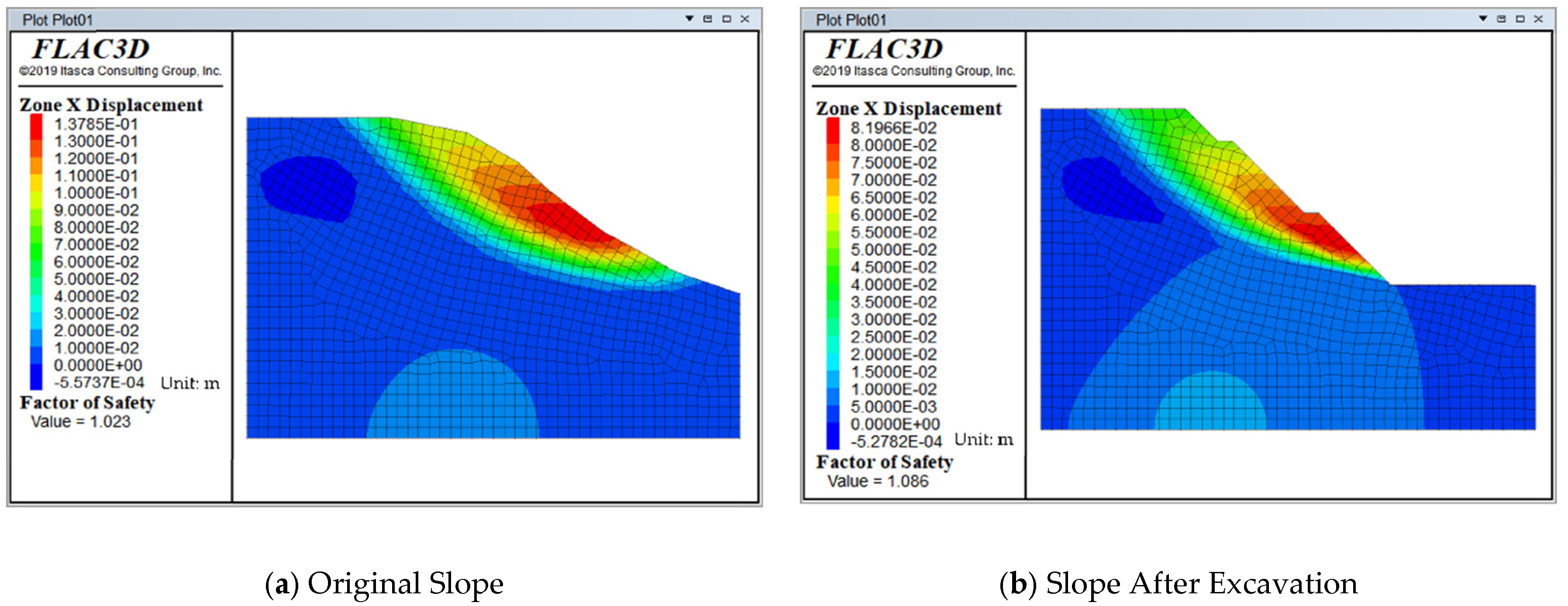
4.2.2. Slope Stability Analysis Before and After Grading

Numerical simulations were conducted using FLAC3D software for both the original slope and the graded slope. The displacement distribution contour maps in the x (horizontal) and z (vertical) directions before and after grading are shown in Figure 23 and Figure 24, respectively.

Based on the displacement monitoring results in Figure 23, the maximum horizontal displacement of the original slope was 13.78 cm (along the positive x-axis). After the excavation treatment, this value decreased to 8.19 cm. The spatial distribution of horizontal displacement shows that the maximum displacement occurred at the middle section of the front edge of the slope before and after the excavation, with the displacement decreasing in both directions from the front edge to the rear edge and from the slope surface to the deep part of the slope body. It is noteworthy that the displacement peak at the front edge of the original slope reached 1.68 times that of the post-excavation condition, indicating that the removal of surface soil at the front edge effectively restrained deformation of the surface layer of the slope.

The vertical displacement analysis in Figure 24 shows that the displacement field before and after excavation has similar spatial distribution characteristics. The maximum settlement is concentrated in the slope top region, with a gradient reduction from the slope top to the toe. Specifically, the maximum vertical displacement of the original slope was 12.77 cm (along the negative z-axis), which decreased to 8.69 cm after excavation, a reduction of 31.9%. Using the FLAC3D strength reduction method, the stability factor of the original slope was calculated as 1.023, which increased to 1.086 after excavation, a 6.15% increase. These data confirm that through slope angle adjustment and removal of surface soil at the front edge, the sliding thrust of the potential sliding mass was effectively reduced, while the stress distribution of the slope body was optimized. This engineering measure improved the overall stability safety margin of the slope by 0.063, creating a favorable support environment for the subsequent construction of the self-drilling anchor support system.

4.3. Analysis of the Supporting Performance of Self-Drilling Anchor Bolts

4.3.1. Orthogonal Experiment on the Impact of Different Support Parameters on Slope Stability

To investigate the influence of anchor rod installation angle, length, and spacing on the stability of slopes when using self-drilling anchor rods for slope reinforcement and to determine the optimal anchor rod support parameters, an orthogonal experiment was designed with three factors and five levels. Additionally, the number of anchor rods per meter of slope was used as the criterion for optimal selection. Numerical simulation analysis was performed using FLAC3D software to solve the slope stability factor. In the simulation, the modified pile element established in Chapter 3 of this study was used for self-drilling anchor rods. The results are shown in

Table 5. Orthogonal experiment scheme and results for different support parameters.

Test Number	Bolt Length (m)	Anchor Angle(°)	Anchor Rod Spacing (m)	Quantity of Anchor Rods (m/per m of Slope)	Safety Factor
1	6	25	1	102	1.3
2	6	30	1.5	68	1.305
3	6	35	2	51	1.294
4	6	40	2.5	40.8	1.287
5	6	45	3	34	1.28
6	7	25	1.5	79.3	1.302
7	7	30	2	59.5	1.303
8	7	35	2.5	47.6	1.301
9	7	40	3	39.7	1.293
10	7	45	1	119	1.4
11	8	25	2	68	1.31
12	8	30	2.5	54.4	1.309
13	8	35	3	45.3	1.311
14	8	40	1	136	1.41
15	8	45	1.5	90.7	1.403
16	9	25	2.5	61.2	1.309
17	9	30	3	51	1.311
18	9	35	1	153	1.416
19	9	40	1.5	102	1.423
20	9	45	2	76.5	1.383
21	10	25	3	56.7	1.313
22	10	30	1	170	1.422
23	10	35	1.5	113.3	1.43
24	10	40	2	85	1.4
25	10	45	2.5	68	1.375

.

4.3.2. Selection of a Support Scheme

The design of anchor rod parameters requires a dynamic balance between safety and economy. For a safety-prioritized solution, it is recommended to use long anchor rods, a moderate angle, and small spacing. For example, the design in experiment No. 23, with a 10-m anchor rod length, 35-degree angle, and 1.5-m spacing, yields a corrected safety factor of 1.430. However, the number of anchor rods is relatively high, reaching 113.3, making it suitable for high-risk slope projects. For an economy-prioritized solution, a combination of short anchor rods, a large angle, and wide spacing may be chosen, such as in experiment No. 5, with a 6-m anchor rod length, 45-degree angle, and 3-m spacing. This results in a lower safety factor of 1.280 but with a significantly reduced anchor rod usage of only 34.0, making it appropriate for low-risk temporary projects.

Considering both the anchor rod usage and safety, we selected the design with a 7-m anchor rod length, 30-degree angle, and 2-m spacing, corresponding to experiment No. 7. This solution achieves a safety factor of 1.303 and an anchor rod usage of 59.5, balancing reasonable safety with cost control.

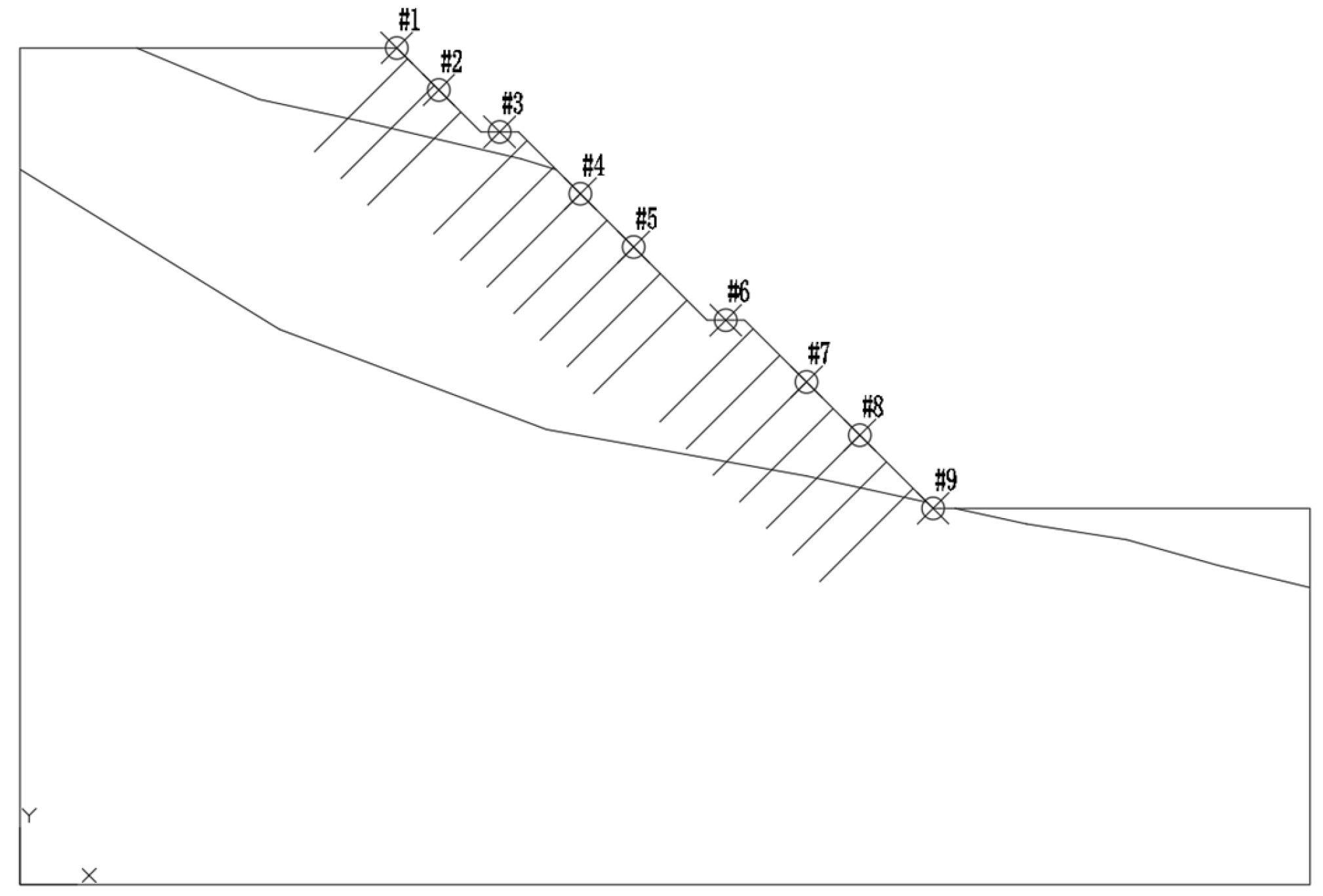
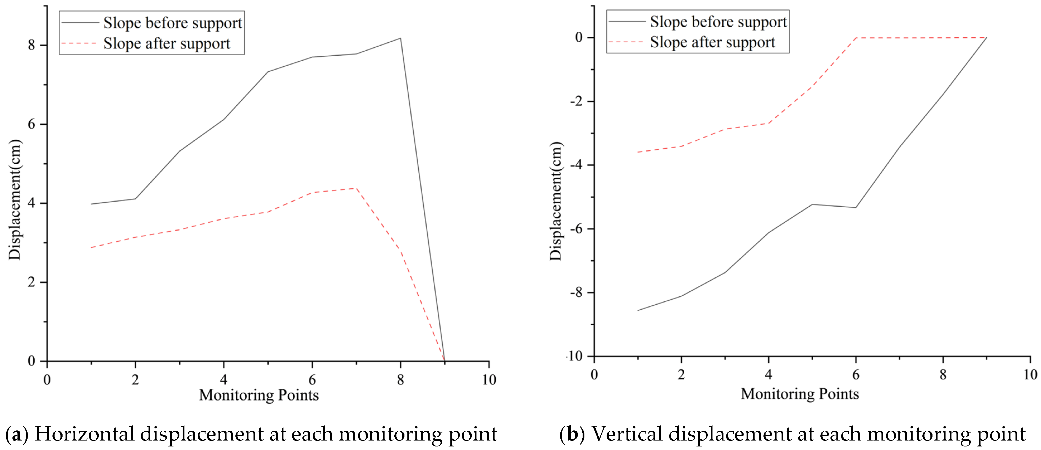
4.4. Stability Analysis of the Reinforced Slope with Self-Drilling Anchors: Displacement Results Analysis

4.4.1. Analysis of the Displacement Results

In the slope model, nine displacement monitoring points were selected along the slope surface, and two monitoring points were set near the slope toe to better analyze the displacement of the soil at the toe. The monitoring points were numbered from 1# to 9#, and the arrangement of model monitoring points is shown in Figure 25.

Numerical simulations were performed using FLAC3D software to analyze the displacement of the slope and self-drilling anchors after reinforcement. The displacement distributions of the slope soil in both the x (horizontal) and z (vertical) directions, along with the displacement changes at each monitoring point, are shown in Figure 26 and Figure 27, respectively.

Observing Figure 26 and Figure 27, it is evident that the displacement of the slope soil at all monitoring points was effectively controlled after the self-drilling anchor support was applied. The horizontal displacement increases as the monitoring points move higher from the slope toe, indicating that the self-drilling anchors significantly reduced the horizontal displacement of the slope soil. Before the support, the maximum horizontal displacement was 8.197 cm, which decreased to 4.408 cm (positive direction of the x-axis) after the support was applied. Notably, at monitoring point 8#, the displacement of the slope soil was considerable, reaching 8.28 cm before the support, with a significant difference in displacement between adjacent points. After the support, the displacement at this point reduced to 2.23 cm, and the displacement difference between adjacent points also decreased. At this point, the maximum displacement of the slope was observed near monitoring point 7, at 4.03 cm.

Figure 26 and Figure 27 also show that, under the support of the self-drilling anchor, the vertical displacement in the z-direction of the slope soil decreased with the elevation of the monitoring points, eventually tending to zero. Compared to the pre-support state, the change is significant. The maximum vertical displacement decreased from 8.694 cm before the support to 3.627 cm (negative direction of the z-axis). At monitoring point 1#, the vertical displacement decreased from 8.56 cm to 3.59 cm. Additionally, it can be observed that there was a sudden change in slope displacement near monitoring point 6# both before and after the support. However, the difference lies in the fact that before the support, the slope displacement gradually decreased as the location approached the slope toe, while under the self-drilling anchor support, the displacement near monitoring point 6# stabilized. This indicates that the self-drilling anchor successfully reduced the vertical displacement tendency of the slope soil, with a clear restraining effect on the soil. The self-drilling anchor support structure prevented the sliding of the slope soil, thereby effectively enhancing the stability of the slope.

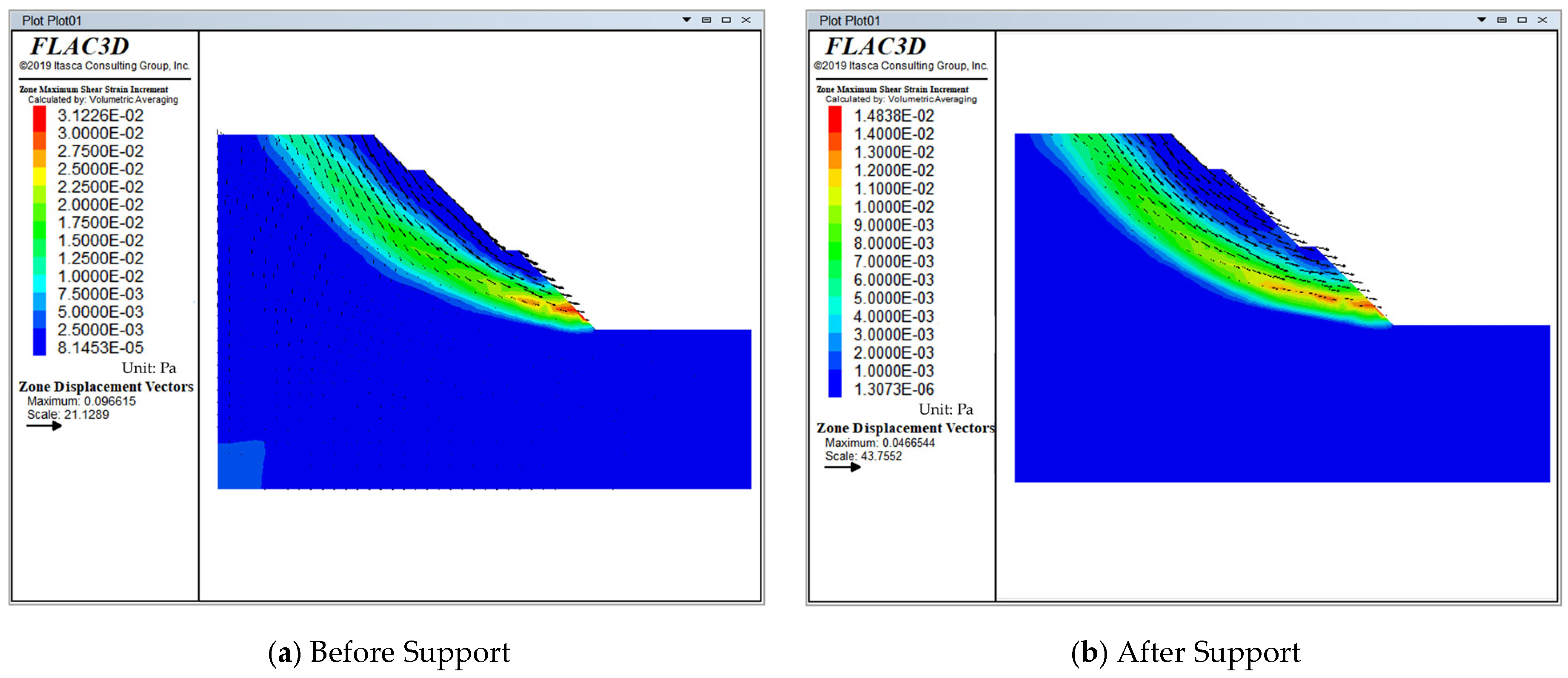
4.4.2. Shear Strain Increment and Velocity Vector Analysis

The distribution of the maximum shear strain increment in the slope soil reflects the stress state of the slope body. By analyzing the maximum shear strain increment distribution, potential sliding surfaces and possible instability modes of the slope soil can be identified. Numerical simulations were carried out using FLAC3D software, and the maximum shear strain increment under self-drilling anchor support was extracted, as shown in Figure 28.

As shown in Figure 28, the maximum shear strain increment of the self-drilling anchors supporting the slope is still distributed at the toe of the slope. However, compared to the unsupported slope, its maximum value decreases from 0.312 to 0.148, representing a 52.6% reduction. This greatly alleviates the sliding tendency of the slope soil, and the shear zone of the slope under the self-drilling anchor bolt support is not significantly penetrated. Additionally, the velocity vector diagram shows that the velocities of the grid points on the potential sliding surface of the slope have significantly decreased. This indicates that the self-drilling anchors support system can improve the distribution of the maximum shear strain increment of the slope, reducing the risk of shear failure at the slope toe, thereby providing a good reinforcing effect on the slope.

5. Conclusions

This study, based on the reconstruction project of an abandoned open-pit mine in Dalian, systematically analyzed the anchoring performance and reinforcement effects of self-drilling anchors in a strongly weathered dolomitic limestone layer using a combination of field pull-out tests and FLAC3D numerical simulations. The main conclusions are as follows:

(1)

The experiments revealed that, under the conditions of grouting pressure at 0.8 MPa and a water-to-cement ratio of 0.8, the average interface bond strength between the self-drilling anchor and the strongly weathered dolomitic limestone reached 0.147 MPa, significantly higher than the recommended value for this stratum (qsk = 0.12 MPa). The test results indicated that the interface shear stress along the anchorage section showed an exponential decay along the axis, with the effective bearing area concentrated near the anchor’s proximal end. The longer anchorage sections reduced randomness due to spatial averaging effects, but the bond strength showed a decreasing trend as the anchorage length increased, validating the “effective anchorage length” theory;

(2)

By incorporating a residual strength model to modify the pile unit in FLAC3D, a more realistic anchorage analysis model was developed. The modified model accurately reflects the nonlinear decay of anchor axial force with depth and the spatial distribution characteristics of interface shear stress. The simulation results closely matched the experimental data, with an error in the ultimate pullout capacity of less than 6%;

(3)

Numerical simulation analysis based on orthogonal experiments showed that anchor length, installation angle, and spacing significantly affected slope stability. Considering both safety and economic factors, it is recommended to use an anchor length of 7 m, an installation angle of 30°, and a spacing of 2 m as the support scheme, which results in an increase in the safety factor to 1.303 and an anchor consumption of 59.5 m/m. After the support, the maximum horizontal displacement of the slope decreased from 8.197 cm to 4.408 cm, and the maximum shear strain increment was reduced by 52.6%, significantly inhibiting the development of potential sliding surfaces.

Finally, we would like to emphasize the limitations of this work and the directions of our future research:

(1)

As the selected working conditions in this paper are highly weathered dolomite strata, which are relatively special, it is currently impossible to determine whether self-drilling anchor rods can have the same or better anchoring performance in other similar geological conditions. Therefore, in our next research, we will conduct studies on the anchoring performance of self-drilling anchor rods under different stratum conditions and multi-layer soil conditions and carry out numerical simulation analysis based on anisotropic stratum conditions. At the same time, the performance degradation of self-drilling anchor rods under the influence of seismic loads is also under consideration in our subsequent work;

(2)

The modified pile element does indeed have a good simulation performance in the simulation, but at the same time, the size effect of the anchor rod will also have a certain impact on the overall anchoring performance. Therefore, it is possible to attempt to use the Zone element combined with the interface method to study the overall anchoring performance of the anchor rod.

References

1. Shi, G.H. Application of self-drilling anchor bars in rock support for Gaomozan Dam. Water Resour. Hydropower Northeast. China 2011, 29, 14–16. [Google Scholar] [CrossRef]
2. Li, X.; Wang, S.S.; Xie, Z.W. Application of self-drilling anchor bars in foundation pit support. Railw. Eng. 2006, 5, 65–66. [Google Scholar]
3. Qi, R.A. Application of self-drilling anchor bars in deep foundation pit support. Constr. Technol. 2014, 43, 111–113. [Google Scholar]
4. Ma, L.; Xu, H. Application of large-diameter self-drilling anchor bars in subway foundation pits. Munic. Eng. Technol. 2014, 32, 129–131. [Google Scholar]
5. Xie, X.L.; Yang, G.Z.; Chen, B. Application of self-drilling anchor bars in slope fractured rock mass and shallow collapse bodies. Sichuan Water Power 2007, 2, 90-92+132. [Google Scholar]
6. Yang, B.; He, B. Application of hollow self-drilling grouting anchor bars in slope support. Sichuan Water Power 2010, 29, 36-38+168. [Google Scholar]
7. Shao, H.Y. Analysis of hollow self-drilling anchor bar technology in slope support engineering. Henan Water Resour. South North Water Divers. 2012, 16, 82–83. [Google Scholar]
8. Wu, H.F. Application of self-drilling anchor bar technology in deep foundation pit support in a mountainous area of southern Anhui. Resour. Inf. Eng. 2023, 38, 79–82. [Google Scholar] [CrossRef]
9. Li, Y.C. Application of self-drilling anchor bars in sand-gravel layer slopes. Site Investig. Sci. Technol. 2012, 6, 24-25+29. [Google Scholar]
10. Ma, W.X.; Xu, Y.B.; Xiao, Z.G.; Fang, Y.M.; Xu, Z.B. Application of self-advancing pipe-roof construction technology in tunnels with weak surrounding rock. Railw. Eng. 2020, 60, 69–72. [Google Scholar]
11. Ministry of Housing and Urban-Rural Development of China. Technical Specification for Retaining and Protection of Building Foundation Excavations (JGJ 120-2012); China Architecture and Building Press: Beijing, China, 2012. [Google Scholar]
12. Tao, Y.W.; Du, Z.G.; Ding, W.X.; Dai, Z.W.; Fu, X.L.; Guo, J.J.; Wei, Y.Q. Experimental study on anchorage bonding performance of BFRP mortar anchor bars. Concrete 2022, 4, 170–175. [Google Scholar]
13. Bai, X.Y.; Zhang, M.Y.; Kuang, Z.; Wang, Y.H.; Yan, N. Load distribution function model for fully-bonded GFRP anti-floating anchor bars. J. Cent. South Univ. (Nat. Sci. Ed.) 2020, 51, 1977–1988. [Google Scholar]
14. Bai, X.Y.; Zhang, M.Y.; Zhu, L.; Wang, Y.H.; Zhao, T.Y.; Chen, X.Y. Experimental study on interfacial shear characteristics of fully-bonded GFRP anti-floating anchor bars. Chin. J. Rock Mech. Eng. 2018, 37, 1407–1418. [Google Scholar] [CrossRef]
15. You, Z.J.; Fu, H.L.; You, C.A.; Zhang, J.; Shao, H.; Bi, D.B.; Shi, J. Stress transfer mechanism in soil anchor systems. Rock Soil Mech. 2018, 39, 85-92+102. [Google Scholar] [CrossRef]
Figure 1. Structural diagram of a self-drilling anchor bolt.
Applsci 15 05132 g001
Figure 2. Drilling process of a hollow self-drilling anchor bolt.
Applsci 15 05132 g002
Figure 3. Qf100-100t hollow hydraulic jack.
Applsci 15 05132 g003
Figure 4. Field test diagram.
Applsci 15 05132 g004
Figure 5. Experimental analysis curves for each set of anchor bolts.
Applsci 15 05132 g005
Figure 6. Graph of the relationship between the increase in ultimate uplift capacity and the decrease in bonding strength.
Applsci 15 05132 g006
Figure 7. Schematic diagram of the mechanism of the pile unit.
Applsci 15 05132 g007
Figure 8. Numerical simulation model diagram.
Applsci 15 05132 g008
Figure 9. Initial displacement cloud.
Applsci 15 05132 g009
Figure 10. Initial stress contour map.
Applsci 15 05132 g010
Figure 11. Residual strength (strain-softening) model.
Applsci 15 05132 g011
Figure 12. Shear stress–displacement curve.
Applsci 15 05132 g012
Figure 13. Modified relationship between ultimate uplift capacity and unit bond strength in pile elements.
Applsci 15 05132 g013
Figure 14. Ultimate uplift capacity–displacement curve.
Applsci 15 05132 g014
Figure 15. Displacement contour map at the ultimate uplift bearing capacity.
Applsci 15 05132 g015
Figure 16. Distribution curve of axial force of anchor rod body.
Applsci 15 05132 g016
Figure 17. Contour plot of anchor axial force at different displacements.
Applsci 15 05132 g017
Figure 18. Stress distribution curve of the anchor–soil interface.
Applsci 15 05132 g018
Figure 19. Soil stress contour map.
Applsci 15 05132 g019
Figure 20. Site exploration map.
Applsci 15 05132 g020
Figure 21. Slope design diagram.
Applsci 15 05132 g021
Figure 22. Numerical Calculation Model.
Applsci 15 05132 g022
Figure 23. Displacement contour in the X direction.
Applsci 15 05132 g023
Figure 24. Displacement contour in the Z direction.
Applsci 15 05132 g024
Figure 25. Layout of displacement monitoring points.
Applsci 15 05132 g025
Figure 26. Displacement cloud maps of the reinforced slope.
Applsci 15 05132 g026
Figure 27. Displacement at monitoring points.
Applsci 15 05132 g027
Figure 28. Maximum shear strain increment and velocity vector diagram of the slope before and after support.
Applsci 15 05132 g028