G-Pre: A Graph-Theory-Based Matrix Preconditioning Algorithm for Finite Element Simulation Solutions

Abstract

In finite element simulation and analysis, increasing simulation scales place high demands on the preconditioning and solution process of linear matrices. However, the most commonly used preconditioning methods for incomplete LU factorization usually increase data access and computation due to data padding and forward/backward operations, as well as affect parallel computing design. To address these challenges, this study proposes a graph–theory-based matrix preconditioning algorithm called G-Pre. In this method, by introducing a graph partitioning algorithm and a graph rearrangement algorithm before ILU factorization, the matrix is partitioned into regions and the elements are rearranged, which improves the ease of data access for matrix computation and facilitates parallel computation. The results of numerical experiments show that in terms of solution efficiency, the solver based on the G-Pre preconditioning algorithm achieved an average speedup ratio of 2.1 and 4.3 times that of the solver based on ILU factorization and the direct solver, respectively. At the same time, the algorithm computed the results with an error of no more than 2%. This method is a novel technique for the matrix preconditioning of finite element solvers and a powerful algorithmic tool to cope with the increasing computational demands of finite element simulations.

1. Introduction

The finite element method (FEM) is a powerful numerical computation technique that is utilized to address complex engineering and physical problems. At its core, the FEM involves discretizing the continuous solution domain into a finite number of elements, establishing approximate solutions within these elements, and employing mathematical tools such as the variational principle or weighted residual method to derive an overall approximate solution for the entire domain. The advancement of electronic computers has facilitated the rapid development of the FEM into a sophisticated computational approach, leading to the emergence of a substantial market for finite element analysis software. In finite element analysis (FEA), many scientific computational projects and practical engineering applications often boil down to solving a system of linear equations with one or more large sparse matrices as the coefficient matrices. The physical properties of the problem and the numerical discretization method determine whether these matrices are symmetric. Symmetric matrices typically arise in problems with symmetric physical properties, such as stiffness matrices in elasticity mechanics, where material–eigen–structure relations are usually invertible and symmetric. Asymmetric matrices generally originate from fluid dynamics problems [1], e.g., convection-dominated problems (CDPs) [2]. When significant convective effects are present (e.g., a high-velocity fluid flow), the discretization of convective terms leads to asymmetry. Additionally, nonlinear Navier–Stokes convective terms can disrupt matrix symmetry. Matrix solution problems are now an essential component of finite element simulation and analysis across various fields, including the automotive [3], aerospace [4], construction [5], semiconductor [6], materials [7], agriculture and forestry [8], and medicine [9] industries. Therefore, efficiently solving the system of linear equations discretized using the finite element method remains a focal point of research in FEA.

At present, many research institutions and scholars, both at home and abroad, have invested a lot of resources in carrying out in-depth research on algorithms for solving systems of linear equations [10,11,12,13,14,15]. The solution algorithms are mainly categorized into two main groups—direct methods [16,17] and iterative methods [18]. The direct method is a numerical method for finding the exact solution of a system of linear equations via finite-step arithmetic operations. However, with the gradual increase in the size of the solving matrix, the conventional direct method is now no longer applicable, and the iterative method is usually used [19]. For cases where the coefficient matrices are symmetric, the conjugate gradient (CG) method is typically applied. This well-known iterative method is effective for solving large sparse symmetric matrix problems [20]. In contrast, when dealing with asymmetric coefficient matrices, the solution approach differs from that used for symmetric matrices. The commonly adopted algorithm in this scenario is the generalized minimal residual (GMRES) method, which is an iterative technique that is specifically designed for solving large sparse asymmetric linear systems [21,22]. However, the convergence behavior of the iterative algorithm depends heavily on the size of the condition number of the correlation matrix [23].

To enhance the stability and speed of the iterative convergence process, matrix preconditioning techniques are often applied [24,25]. This technique transforms the initial system of linear equations by constructing a preprocessor M, which is equivalent to the initial system of linear equations; then, the resulting new system of linear equations for computation is solved [26]. This conversion process aims to make the distribution of the eigenvalues of the coefficient matrix of the new system of equations more centralized, which, in turn, speeds up the convergence rate. The preconditioning technique is crucial for the successful application of the iterative method in real-world problems and has become one of the research hotspots for the efficient solution of sparse linear systems of equations [27]. There are various methods for constructing preprocessors, including incomplete LU (ILU) factorization preconditioning [28], sparse approximate inverse (SPAI) [29], polynomial preconditioning, classical iteration-based Jacobi [30], and symmetric successive over-relaxation (SSOR) [31] preconditioning. Among these methods, ILU factorization preconditioning has the advantages of low construction costs and a wide range of applications, and it can be adjusted by filling the parameters; however, it also encounters problems, whereby some indeterminate matrices cannot be applied and the storage computation is difficult to predict. The advantages of approximate inverse preconditioning are its good convergence and parallelism, as well as its ease of applicability; however, the construction and storage costs are too high and are not suitable for large-scale matrices. The advantages of polynomial preconditioning are that it is simple and easy to implement, and no matrix factorization is needed; however, the preconditioning effect is general and the convergence speed is slow. The advantages of the Jacobi method are that it is simple and easy to implement, but its convergence speed is slow, its preconditioning effect is limited, and it is only applicable in the case of the diagonal dominance of matrices. The advantages of the SSOR method are that it accelerates the convergence through the introduction of the relaxation factor w and that the iteration process is more stable, but it introduces additional computational effort, which is not suitable in the case of large-scale matrices. However, it introduces additional computational effort, which may lead to longer computation times when encountering large-scale matrix computation and is not suitable for asymmetric matrices. In practice, ILU factorization has become one of the most widely used preconditioning methods due to its good balance and scalability, wide range of applications, and mature technology development [32].

ILU factorization is a commonly used preconditioning technique, developed on the basis of standard LU factorization. The method reduces the computation and storage space by retaining only some non-zero elements in the factorization process, before obtaining the product of the lower triangular matrix L and the upper triangular matrix U in order to approximate the original matrix A. ILU factorization has a good preconditioning effect for both symmetric and asymmetric matrices. In practice, by discarding some elements, ILU factorization effectively weakens the fill-in phenomenon in the factorization process, further reducing the use of storage space. Among them, the commonly used ILU factorization has various forms. One of the standard and widely adopted padding selection methods is ILU (0) [33], which fills in zeros during the factorization process. Krylov subspace iterative solvers preprocessed with ILU (0) are extensively used across various engineering disciplines. Other commonly utilized padding selection methods include ILUT and ILUC [34,35]. Additionally, ILUB, which leverages single instruction–multiple data (SIMD) instructions for enhanced performance, has been proposed [36]. However, in practice, conventional ILU factorization is difficult to parallelize and does not meet the demands of modern large-scale computation. The ILU factorization method with increased padding levels may change in accordance with the padding level, which, in turn, leads to a large change in the amount of storage and operations, making it difficult to control the factorization effectively. If zero padding is used, the element rounding of the matrix will also be further increased, which, in turn, amplifies the error of the factorization matrix. To address these problems, there is an urgent need to develop new techniques to optimize the effect of ILU factorization, reduce the error, and achieve parallel computing, enabling effective control of changes in storage and computation.

With the widespread application of graph theory techniques in matrix processing, numerous matrix preconditioning algorithms based on graph–theoretic methods have been developed, which has also led to research in the direction of solving the above problems. For instance, Daniel Osei-Kuffuor et al. [37] introduced an efficient graph reordering algorithm that is grounded in graph theory. This algorithm optimizes matrices following ILU decomposition preconditioning through a multilevel graph coarsening strategy, significantly enhancing solution stability and processing speed. However, the method is somewhat limited in terms of applicability, and to apply it to a wider range of problems would require adjusting the parameter settings and increasing the complexity, which contradicts our idea of wanting to simplify preconditioning. Subsequently, Zheng Qingqing et al. [38] proposed a graph–theoretic method for matrix reordering. Their approach effectively reorders sparse matrices by constructing a two-layer chunked diagonal framework through the poly-chromatic coloring of subdomain adjacency graphs. However, its current applicability is still insufficient for the vast majority of symmetric and asymmetric problems. In this paper, an efficient matrix preconditioning algorithm, G-Pre, is developed by adding a graph partitioning algorithm and a graph reordering algorithm before the ILU factorization process. The algorithm implements the partitioning and concentration of non-zero elements of the matrix, which allows the ILU factorization to be executed in parallel in different partitions and improves the computational data access efficiency. The feasibility of the proposed algorithm is demonstrated through numerical experiments.

The rest of the paper is structured as follows. In Section 2, symmetric and asymmetric matrix solution problems are briefly introduced with examples of static analysis problems and fluid dynamics problems. Then, commonly used solution algorithms and preconditioning methods for symmetric and asymmetric matrices are reviewed. Section 3 presents the preconditioning algorithm based on graph theory. Section 4 details the numerical experimental procedure and an analysis of the results, testing the effectiveness of the preconditioning algorithm using an actual finite element simulation model. Finally, Section 5 discusses related work and concludes the study.

2. Methods

2.1. Problems in Solving Systems of Linear Equations in Finite Element Analysis

In FEA, many scientific computational projects and practical engineering applications are often reduced to solving a system of linear equations with one or more large sparse matrices as coefficient matrices, as follows:

$$\mathit{Ax}=\mathit{b},$$

(1)

where A represents the coefficient matrix of the system of linear equations, and b is a vector. The physical properties of the problem and the numerical discretization method determine whether the coefficient matrix is symmetric. For different types of coefficient matrices, distinct solution methods are employed.

2.1.1. Asymmetric Matrix Solution Problem

Asymmetric matrices generally appear in fluid problems. Fluid problems involve the study of fluid (liquid or gas) behavior and properties under various physical conditions through mathematical modeling and numerical calculations; they encompass application scenarios such as semiconductor devices [39,40], multiphysics field coupling [41,42], and complex geometries [43]. The complex and varied application scenarios, as well as the increasing interest in fluid problems, have put higher computational demands on asymmetric matrix solving. In addition, the complex working conditions in fluid problems also bring difficulties and challenges to asymmetric matrix solving. For example, in the convective dominance problem [2], a system of asymmetric linear equations is obtained by processing the finite element discretization of the convective term, as well as the partial integration of the diffusion term, in the convective diffusion equation [44], as follows:

$${\displaystyle \frac{\partial \mathit{u}}{\partial \mathit{t}}}+\mathrm{v} · \mathsf{\nabla }\mathit{u}=\mathsf{ϵ}{\mathsf{\nabla }}^{ 2}\mathit{u}+\mathit{f},$$

(2)

This leads to the following system of asymmetric linear equations:

$$\left(\mathrm{C}+\mathsf{ϵ}\mathrm{K}+\mathsf{\tau }{\mathrm{C}}_{\mathrm{stab}}\right)\mathrm{u}=\mathrm{F}+\mathsf{\tau }{\mathrm{F}}_{\mathrm{stab}},$$

(3)

where $\mathit{A} =\mathrm{C}+\mathsf{ϵ}\mathrm{K}+\mathsf{\tau }{\mathrm{C}}_{\mathrm{stab}}$ and $\mathit{b} =\mathrm{F}+\mathsf{\tau }{\mathrm{F}}_{\mathrm{stab}}$. The combination of these two gives the following linear system: Au = b. The complex matrix composition requires that the matrix preconditioning and solving methods must also be efficient and reasonable; only in this way can we meet the growing demand for solving asymmetric matrices. Consequently, developing efficient methods for solving asymmetric matrices is a key research direction in the simulation process.

2.1.2. Symmetric Matrix Solution Problem

Symmetric matrices are most commonly used in the static analysis of structures. Static analysis is a fundamental aspect of structural mechanics [45] and is widely employed in engineering to assess changes in structural response under static loads. In static analysis, solving the stiffness matrix that is obtained by discretizing the three fundamental equations of elasticity mechanics (equilibrium, constitutive, and geometric equations) is essential. The stiffness matrix is typically a large sparse matrix, with over 30% of its elements being zeros. This special matrix structure results in a low data access hit rate during the solving process, significantly affecting efficiency. However, it also provides opportunities for improving memory access continuity, which can accelerate the solving process. Directly applying solution algorithms without considering these characteristics often leads to prolonged solution times, poor convergence performance in iterative processes, and a slow simulation process. Therefore, the preconditioning of sparse matrices must consider the effects of matrix sparsity to optimize performance.

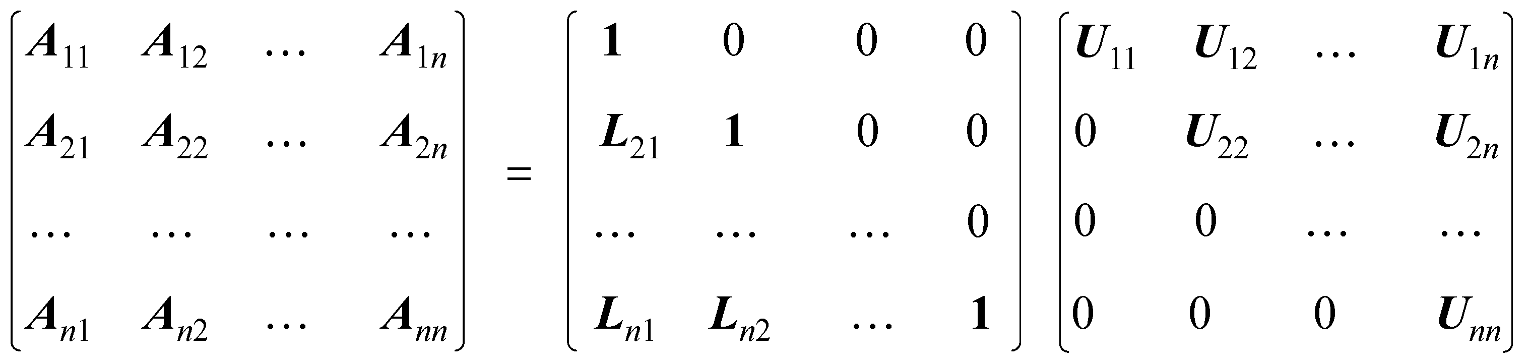
2.2. Matrix Solving Algorithm

Many solution methods have been developed for matrix solving problems. Among them, iterative methods are more suitable for large-scale matrix solving problems due to the advantages of low storage requirements and the easy implementation of algorithms. Commonly used iterative methods for solving symmetric matrices include the CG method [46], the Jacobi iteration method [30], the Gauss–Seidel iteration method [47], and the successive over-relaxation (SOR) iteration method [31]. The Jacobi iteration method has the advantage of simplicity and ease of implementation, but its convergence speed is slower, and it is only suitable for the case of the diagonal dominance of the matrices. The Gauss–Seidel iteration method usually converges faster than the Jacobi iteration method, but it requires more time and computation to implement the algorithm. The SOR method requires the selection of a suitable relaxation factor w in order to effectively improve the convergence speed. The conjugate gradient method is an efficient stepwise approximation method that only needs to utilize the first-order derivative information and does not need to compute and store the Hesse matrix and its inverse matrix, thus reducing the high computational cost of Newton’s method. At the same time, it overcomes the disadvantage of the slow convergence of the most rapid descent method, which is a very effective approach to solve large sparse symmetric matrix solution problems [20]. In asymmetric matrix solving problems, the most commonly used methods include the QR decomposition method [48], GMRES [21,22], and the biconjugate gradient stabilized (BiCGStab) method [49]. Among these, the former has a high computational complexity, usually O (n³), and a low computational efficiency, which is not applicable for solving large-scale matrices. Although the stabilized dual conjugate gradient method converges faster, it is prone to the phenomenon of iterative oscillation and abnormal residual values, relying less on the preconditioning technology, which cannot effectively reflect the practical effect of the preconditioning algorithm proposed in this paper. As a mature iterative method, the generalized minimum residual method has better applicability and convergence, and the iterative process is more stable. Therefore, in this test study, CG and GMRES were used in order to fully verify the effectiveness of the preconditioning algorithm G-Pre that is proposed in this study.

GMRES is an iterative technique for solving large sparse asymmetric linear systems of the form Au = b. The core idea is to find an approximate solution that minimizes the residual $r=‖b-\mathit{Au}‖$ by constructing the Krylov subspace ${\mathit{K}}_{\mathit{m}}\left(\mathit{A}, {\mathit{r}}_0\right)=\mathit{span}\left\{{\mathit{r}}_0, \mathit{A}{\mathit{r}}_0,{\mathit{A}}^2{\mathit{r}}_0,\dots ,{\mathit{A}}^{\mathit{m}-1}{\mathit{r}}_0\right\}$ within this subspace [21,22]. The flow of the GMRES algorithm is as follows.

It starts with an initial estimate of the solution u₀ and computes the following initial residual:

$$r_0=b - A{u}_0.$$

(4)

Let $\mathsf{\beta }=\left|\right|r_0\left|\right|$ and set the basis vector as follows:

$$v_1=r_0/\mathsf{\beta }.$$

(5)

The Arnold process is performed to construct orthogonal bases. For j = 1, 2, …, m, the following is computed:

$$w =A{v}_j.$$

(6)

Orthogonalizing w with all previously generated basis vectors v₁, …, v_j using the modified Gram–Schmidt process, we obtain the following:

$$h_{i,j}=v_i^{j}w,$$

(7)

$$w=w - h_{i,j}{v}_i, (i=1,2,\dots ,j).$$

(8)

Computing $h_{j+1,j}=‖w‖$ and normalizing, we obtain the following new basis vector:

$$v_{j+1}=w/h_{j+1,j}.$$

(9)

Then, we construct the upper Hessenberg matrix $H_m\in R^{\left(m+1\right)\times m}$ (consisting of h_i,j) and minimize the residuals by solving the following least squares problem:

$$y_m=\mathit{arg}\underset{y}{\mathit{min}}\mathsf{}‖\mathsf{\beta }{e}_1-H_{m}y‖,$$

(10)

where $e_1={\left[1,0,\dots ,0\right]}^{\mathrm{T}}\in {\mathrm{R}}^{m+1}$.

Updating the solution, we obtain the following approximate solution:

$$u_m=u_0+V_m{y}_m,$$

(11)

where $V_m=\left[v_1,v_2,\dots ,v_m\right]$. If the iterative process does not converge, the iteration is restarted by resetting the subspace dimension m with u_m as the new initial solution.

By following these steps, GMRES iteratively refines the solution until the desired accuracy is achieved. The algorithm implementation is shown in Algorithm 1.

Algorithm 1: GMRES.

Input: Initial value u0, Convergence boundary Ɛ > 0, Maximum number of iterations IterMax 1: r0 = b − Au0, β = ||r0||2 2: υ1 = r0/β 3: for j = 1, …, IterMax: 4:   w = Avj 5:   for i = 1, …, j: 6:      hi,j = (vj,w) 7:      w = w − hi,j vi 8:   end for 9:  hj+1,j = ||w||2 10:   if hj+1,j = 0: 11:      m = j, break 12:   end if 13:   vj+1 = w/hj+1,j 14:   relres = ||rj||2/β 15:   if relres < Ɛ: 16:    m = j, break 17:  end if 18: end for

The CG method is a well-known iterative algorithm for solving large sparse symmetric matrix problems. The algorithm begins with an initial estimate x₀ of the vector x and iteratively generates a series of approximate solutions within the Krylov subspace. The flow of the algorithm proceeds as follows.

An initial estimation of the solution u₀, as well as the calculation of residuals and initial search direction, is as follows:

$$r_0=A{x}_0 - b,$$

(12)

$$P_0=-r_0.$$

(13)

The calculation factor α is as follows:

$${\mathsf{\alpha }}_k={\displaystyle \frac{r_k^T·r_k}{P_k^T·A·P_k}}.$$

(14)

Updating the solutions and residuals, we obtain the following:

$$x_{k+1}=x_k+{\mathsf{\alpha }}_k·P_k,$$

(15)

$$r_{k+1}=r_k+{\mathsf{\alpha }}_k·P_k.$$

(16)

Then, the coefficient β and the new search direction are calculated, as follows:

$${\mathsf{\beta }}_k={\displaystyle \frac{r_{k+1}^T·r_{k+1}}{r_k^T·r_k}},$$

(17)

$$P_{k+1}=-r_{k+1}+{\mathsf{\beta }}_k·P_k.$$

(18)

The relative residuals are then calculated and compared with the convergence bounds, as follows:

$$r^{’}={\displaystyle \frac{b -A{x}_k}{b}}.$$

(19)

where k = 0, 1, 2, … denotes the number of iterations. The specific algorithmic procedure is shown in Algorithm 2.

Algorithm 2: CG.

Input: stiffness matrix A, load vector b, initial value x0, convergence bound Ɛ, Maximum number of iterations IterMax. 1: r0 = Ax0 − b, P0 = − r0 2: α0 = ||r0||/P0TAP0 3: while || Axk − b ||/||rk|| > Ɛ: 4:   for k = 1, …, IterMax: 5:      xk = xk−1 + αk−1Pk−1 6:      rk = rk−1 − αk−1APk−1 7:      βk−1 = ||rk||/||rk−1|| 8:      Pk = rk + βk−1Pk−1 9:   end for 10: end while

2.3. Matrix Preconditioning Algorithm

To solve large sparse matrices, iterative methods are a better choice. However, the large condition number of large sparse matrices significantly affects the stability, efficiency, and convergence of these iterative methods, which seriously hinders their application in finite element simulation. The convergence characteristics of iterative methods are generally related to the distribution of the eigenvalues of the coefficient matrix of a system of linear equations, especially for Krylov subspace methods. The convergence of these methods is closely related to the density of the eigenvalues of the coefficient matrix; the more concentrated the distribution, the faster the convergence speed [50]. Preconditioning techniques are acceleration methods that are designed to improve the convergence characteristics of iterative methods. These techniques construct a preconditioner M through the incomplete factorization of matrix A, transforming the original system of linear equations into an equivalent new system. This transformation makes the distribution of the eigenvalues of the coefficient matrix in the new system more concentrated, thereby improving the convergence performance of the iterative solver. Preconditioning techniques are crucial for the successful application of iterative methods in practical problems and have become one of the hot spots in the research of the efficient solving of sparse linear equations [27]. Additionally, the combination of preconditioning techniques and Krylov subspace projection methods is considered to be the best “general” iterative solving method [34].

For commonly used iterative algorithms, it is essential to establish a suitable preconditioner to improve the condition number of the coefficient matrix A. This improves the number of iterations required, accelerates convergence, makes the iterative process more stable, and reduces computational cost. Preconditioning technology is the core means to accelerate the convergence of iteration. The most commonly used preconditioning method is ILU factorization.

ILU factorization is an enhancement of LU factorization, as illustrated in Figure 1. ILU is a preconditioning method that reduces computational and storage overhead by retaining only some non-zero elements, while decomposing matrix A into an approximate product of a lower triangular matrix L and an upper triangular matrix U. This method can effectively mitigate the fill-in phenomenon and reduce memory requirements.

Generally, there are two main approaches to preconditioning using incomplete LU factorization.

• Multilevel incomplete factorization (ILU(l)): This approach, denoted as ILU(l), is based on symbolic factorization, which computes the hierarchical level l of the non-zero elements in the factorization from the non-zero structure of the original matrix A. Elements with a hierarchical level l greater than a specified threshold are discarded [51]. The hierarchical value of the non-zero elements in the factorization is solely dependent on the distribution of the non-zero elements in A and is independent of their actual values. If matrix A is diagonally dominant, the elements at higher levels in the factorization tend to have smaller absolute values during LU factorization. Thus, in incomplete factorization, elements with level values exceeding a given threshold can be discarded [50]. However, for matrices without diagonal dominance, this relationship does not hold, and discarding elements based purely on their hierarchical level may result in unreliable preconditioners due to ignoring the impact of element values [34].
• Threshold rounding strategy: Another approach involves using a threshold rounding strategy based on the numerical magnitude of the elements in the factorization [52]. Given a threshold value τ > 0, non-zero elements in the factorization are discarded if their absolute value is less than τ; otherwise, they are retained. Although the relationship between the magnitude of discarded elements and the number of iterative steps required for convergence is complex, generally, discarding fill-in elements with smaller absolute values produces higher-quality preconditioners compared to discarding elements with larger values [27].

It should be noted that both methods of constructing preconditioners face challenges related to unpredictable amounts of fill-in data, leading to increased computational effort.

Preconditioning technology is key to efficiently solving systems of linear equations. We designed a G-Pre preconditioning algorithm based on graph partitioning, graph reordering, and ILU factorization, which combines graph partitioning suitable for parallelism, as well as a graph reordering algorithm focusing on non-zero elements to speed up the computation. We also used ILU factorization, which is suitable for solving linear systems. The computational cost and memory requirements are lower and can accelerate the convergence speed of the iterative method effectively in order to improve the convergence speed of the method and the stability of the iterative process.

3. Graph Theory and G-Pre Preconditioning Algorithm Design

3.1. Graph Theory

Graphs are ubiquitous in scientific computing. For example, a discretized lattice of partial differential equations can be conceptualized as a graph. Similarly, the sparse structure of a sparse matrix can be represented graphically. Graph partitioning and reordering are important problems in various fields, including scientific computing, VLSI design, geographic information systems, operations research, and mission planning [53]. During the iterative solution of systems of linear equations in finite element methods, a key step in each iteration involves the product of sparse matrices and dense vectors. However, the sparse structure of the stiffness matrix and the intrinsic algorithmic properties of sparse matrix vector multiplication (SpMV) result in significant data storage requirements and low cache hit rates. This situation provides an opportunity to increase computational speed by enhancing the continuity of memory access. The SpMV process for sparse matrices is shown in Figure 2, where the black squares represent non-zero elements in the vector and a row of the matrix, and the light-colored areas represent a row of the matrix and a column of the vector. For each calculation, a single row of matrix M is multiplied by the elements in vector V. The relevant data are read according to the position of the non-zero elements in the rows of matrix M. The vector T is then obtained by multiplication and accumulation. The challenge of graph partitioning arises when solving the sparse system Ax = b in parallel. Graph partitioning is a crucial preconditioning stage in high-performance parallel computing. Efficient graph partitioning and the reordering of the graph associated with matrix A can distribute the computational workload evenly across computing nodes and significantly reduce communication overhead during parallel SpMV operations [54].

In this study, the graph partitioning algorithm METIS [53] was utilized. METIS is a well-known algorithm that divides graph nodes into cohesive clusters to effectively minimize edge cuts (defined as the number of edges connecting different clusters). The overall graph partitioning phase consists of three stages—coarsening, division, and refinement. In the reordering phase, the graph is partitioned using a multilevel full set of dissection strategies, and the number of partitions divided depends on the actual situation. Taking a graph divided into two subdomains as an example, as shown in Figure 3. The original graph region contains seven nodes, and the nodes are connected with edges. When the graph is divided and rearranged, each node has a different sequence number, the node with the most connected edges (the red node in Figure 3) is usually selected for division. When the graph is divided into two different subdomains, the nodes within the same subdomain are sequentially renumbered to create a reordered mapping to minimize the filling of sparse matrices [55]. As shown in Figure 4, graph reordering can be categorized as full graph reordering or partition reordering. Figure 4b represents full graph rearrangement, i.e., the rearrangement of elements in the entire graph. Full graph rearrangement results in a tightly arranged block of non-zero elements, and although it also centralizes the non-zero elements, having only one block of elements is not conducive to parallel computation. Figure 4c represents partitioned rearrangement, where the graph is first partitioned and then subdivided so that tightly arranged blocks of elements can be obtained in different partitions; this is favorable for parallel computation. Through graph partitioning and reordering, a reordered matrix with multiple partitions is obtained, where non-zero elements are tightly arranged. This arrangement facilitates the subsequent iterative solving process. In the pre-factorization and solving stage, the challenge of parallelism due to forward/backward substitution during the ILU factorization process is effectively mitigated by assigning matrix blocks from different partitions to different processor cores for factorization and solving computations. To address communication issues between different partitions, boundary node communication can be employed. Specifically, each partition’s boundary nodes interact with neighboring partitions through transfer interfaces such as MPI, ensuring efficient data exchange and synchronization.

3.2. G-Pre Preconditioning Algorithm Design

The speed of the solution iteration significantly determines the overall efficiency of the simulation and analysis. However, the iterative convergence process is influenced by various factors, with the preconditioning effect on the coefficient matrix being one of the key determinants. To enhance the preconditioning effect, this section introduces a preconditioning algorithm called G-Pre. It consists of the following three main stages:

• Preconditioning division and reordering stage: This stage divides and reorders the matrix using a graph partitioning algorithm.
• Preconditioning factorization stage: In this phase, the ILU algorithm is employed to factorize the matrix.
• Parallel solving stage: The preprocessed matrix is then solved through parallel iterations.

By integrating graph theory algorithms with ILU factorization, the matrix structure can be effectively improved, facilitating parallel computation and enhancing the efficiency of matrix solving. These improvements will be demonstrated through numerical experiments in Section 4.

An efficient preconditioning algorithm named G-Pre has been developed for solving systems of finite element linear equations by integrating three methodologies—graph partitioning, graph reordering, and ILU factorization. The G-Pre algorithm comprises three main stages—a partitioning stage, a matrix reordering stage, and a factorization stage; these are followed by an iterative solving stage, where the final solution to the original matrix is obtained through iterative computations. The partitioning stage utilizes a graph partitioning algorithm to divide the computational domain into cohesive subdomains, minimizing edge cuts between different clusters. This step ensures balanced workload distribution across processors in parallel computing environments. The matrix reordering stage applies a graph reordering algorithm to sequentially renumber nodes within each subdomain, aiming to reduce fill-in during the subsequent factorization process. Finally, the factorization stage employs ILU factorization to prepare the matrix for efficient iterative solving. Algorithm 3 illustrates the code implementation process of the G-Pre preconditioning algorithm, using the GMRES algorithm as an example to demonstrate how these stages are integrated to solve the system of linear equations iteratively.

Algorithm 3: G-Pre code process.

Input: Non-symmetric matrix A, right-hand side vector b, initial guess x0, tolerance tol, max iterations max_iter Output: Approximate solution x 1: Step 1: Graph theory preconditioning 2: function preprocess_with_METIS(A): 3: graph = extract_graph(A) 4:  n_partitions = calculate_optimal_partitions(A) 5:  partition_result = METIS_PartGraph(graph, n_partitions) 6:  P = construct_permutation_matrix(partition_result) 7:  A_permuted = P.T @ A @ P 8:  preconditioners = [] 9:  for i in 0 to n_partitions − 1: 10:   block = extract_block(A_permuted, i) 11:   M_i = ILU(block) 12:   preconditioners.append(M_i) 13:  return P, preconditioners 14: Step 2: Preconditioned GMRES solver 15: function METIS_preconditioned_GMRES(A, b, x0, tol, max_iter): 16: P, preconditioners = preprocess_with_GRF(A) 17: b_permuted = P.T @ b 18: x = P.T @ x0 19: r = b_permuted − A_permuted @ x 20: beta = norm(r) 21: Q = [r/beta] 22: H = empty_matrix 23: for j in 0 to max_iter − 1: 24:  v = apply_preconditioner(Q[j], preconditioners) 25:  w = A_permuted @ v 26:    for i in 0 to j: 27:   H[i, j] = dot(Q[i], w) 28:   w = H[i, j] ∗ Q[i] 29:    H[j + 1, j] = norm(w) 30:    Q.append(w/H[j + 1, j]) 31:    e1 = [beta, 0, …, 0].T 32:    y = solve_least_squares(H [0:j + 2, 0:j + 1], e1) 33:    residual = norm(H [0:j + 2, 0:j + 1] @ y − e1) 34:    if residual < tol: 35:   break 36: x_update = P @ (Q [0:j + 1] @ y) 37: x = x0 + x_update 38: return x 39: function apply_preconditioner(v, preconditioners): 40:    z = zeros_like(v) 41:    for i in 0 to len(preconditioners) − 1: 42:   block_indices = get_block_indices(i) 43:   z[block_indices] = preconditioners[i].solve(v[block_indices]) 44:    return z

4. Numerical Experimental Simulation and Analysis

After developing the G-Pre preconditioning algorithm, numerical experimental simulations were conducted to evaluate its performance by comparing it with the ILU factorization solution process. In this section, we present the findings in detail. Firstly, the effectiveness of the G-Pre algorithm was verified and analyzed using asymmetric matrices. Subsequently, the G-Pre algorithm was integrated into the finite element simulation process of a real model and was tested using a realistic mesh model under static analysis conditions. The G-Pre algorithm was implemented in C++. All experiments were performed on a system equipped with a 12-core Intel Core i7-12700 processor and 32 GB of RAM (Intel, Santa Clara, CA, USA). The results, as shown in the related graphs, illustrate the running times of the corresponding experiments. Unless otherwise stated, the relative tolerance convergence bounds for all iterative algorithms in the numerical experiments were set to 10⁻⁵.

4.1. Introduction to Test Models

To evaluate the effectiveness of the proposed G-Pre preconditioning algorithm and to simplify the testing process, we selected a total of four asymmetric matrix solver models with varying scales. These models were used to assess the solving performance of the G-Pre algorithm. The relevant information for each model is summarized in

Table 1. Model and matrix information.

No.	Matrix Dimension	Non-Zero Elements
1	1565	78,425
2	26,742	1,362,615
3	475,750	24,262,002
4	3,843,405	196,012,424

.

4.2. Comparison of Results

In the matrix solving process, several factors influence the solution efficiency, stability, and convergence. These factors include the following:

• A comparison and analysis of condition numbers;
• Solving time comparisons;
• Analysis of the distribution of matrices after preconditioning;
• Convergence performance during the matrix solving process;
• Accuracy of the matrix solving results.

To ensure the stability and reliability of the solving tests, the same model was solved multiple times under each solving condition. Relevant data were recorded across these runs, and the results were compared and analyzed using their average values.

4.3. Algorithm Performance Analysis

4.3.1. Comparison of Matrix Condition Numbers

In the solution process of a linear system, the size of the condition number can be used to measure the stability of the matrix under numerical operations. The larger the condition number, the more unstable the matrix A becomes during numerical computation; that is, a small change in the input data may lead to a significant change in the output result. For a given matrix A, the condition number is defined as follows:

$$\mathsf{\kappa }\left(\mathit{A}\right)=‖\mathit{A}‖·‖{\mathit{A}}^{-1}‖$$

(20)

where ||A|| is some norm of matrix A (usually Manhattan, Euclidean, or maximal), and ||A⁻¹|| is the corresponding norm of the inverse matrix of A. The condition number κ(A) can be any positive real number, including infinity.

The condition numbers of the matrix A in its initial state were compared with those after preconditioning using ILU and G-Pre, respectively. The results are shown in

Table 2. Comparison of matrix condition numbers.

Matrix	Original	ILU	G-Pre
Matrix 1	1.2297 × 108	7.8489 × 105	6.5499 × 102
Matrix 2	2.5738 × 1029	1.3881 × 1021	9.8851 × 104
Matrix 3	4.6577 × 1043	3.5248 × 1032	1.3415 × 1015

. In the initial case, the condition numbers of the different matrices were very large, leading to instability during numerical computation. However, after preconditioning, the condition numbers of the matrices were reduced to some extent. Specifically, the G-Pre preconditioning algorithm significantly outperformed ILU factorization in optimizing the condition numbers. For several matrices in this test, the G-Pre preconditioning algorithm improved the condition number by an average factor of 2.6 compared to that of ILU factorization. Lower condition numbers also imply higher stability in the solving iteration process for G-Pre, as will be demonstrated in the convergence performance comparison during the matrix solving process.

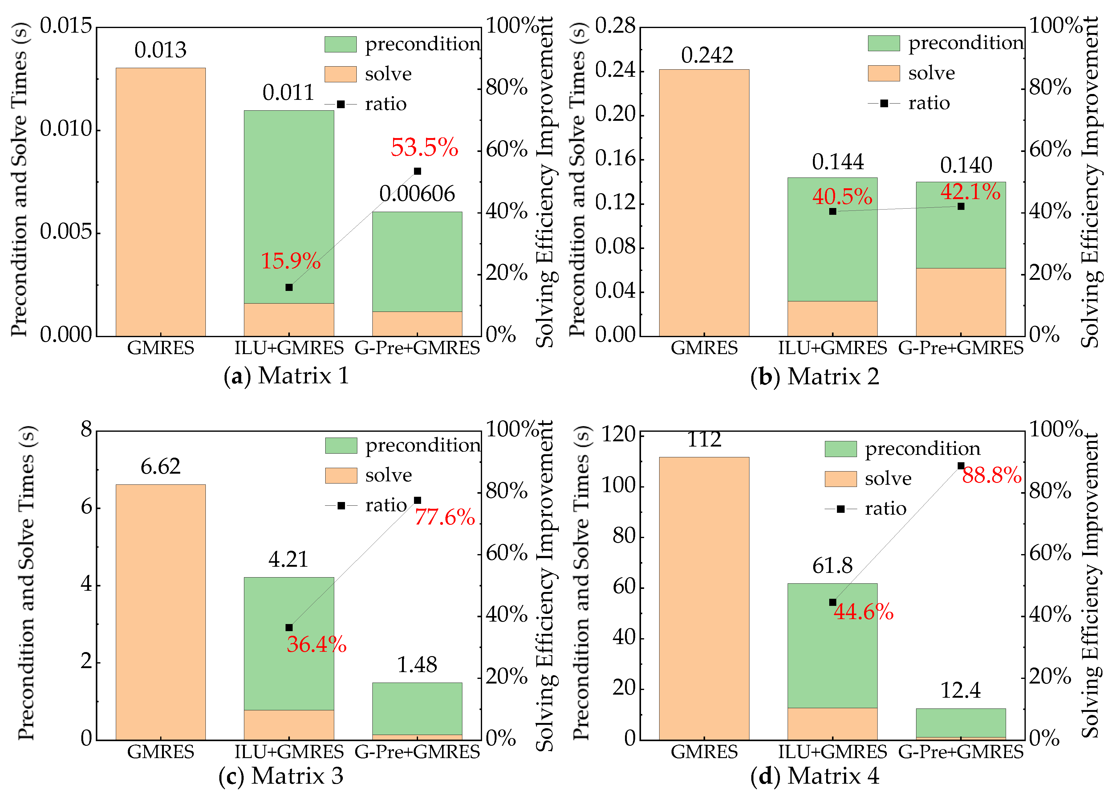
4.3.2. Comparative Analysis of Solving Time After Preconditioning Optimization

Solution efficiency is a crucial metric for assessing the performance of a solver, with the duration of the solving time directly impacting the progress of simulation projects. The most straightforward way to compare solution efficiency is by directly comparing the solving times. For methods that use iterative solvers without preconditioning, the total time consists solely of the matrix iteration solving time. In contrast, for solvers that incorporate preconditioning, the total time includes two components—the preconditioning time and the subsequent matrix solving time. The effectiveness of the preconditioning step depends on whether the sum of the preconditioning time and the matrix solving time can outperform direct solving using an iterative method.

To evaluate the effectiveness of the G-Pre in accelerating the solution of matrix problems, we compared the total solving time, preconditioning time, and solving time with those of two different cases—no preconditioning and ILU factorization. Solving experiments were performed on the four matrices described in Section 4.1, and the results are presented in Figure 5. The efficiency of matrix solving was significantly improved with preconditioning, and both the overall time and the solving time for G-Pre preconditioning and ILU factorization were considerably reduced compared to the case without preconditioning.

In the four matrix-solving tests, the efficiency of G-Pre solving improved by 53.5%, 42.1%, 77.6%, and 88.8%, respectively, compared to solving directly with GMRES, and improved by 44.9%, 2.8%, 64.8%, and 79.9%, respectively, compared to solving with ILU factorization. Comparing G-Pre preconditioning and ILU factorization, G-Pre preconditioning exhibited greater speedup, more than doubling the performance for matrices 3 and 4, indicating higher solution efficiency in G-Pre.

However, when comparing matrices 1 and 2, the solving times were similar for both methods when the matrix size was small. In addition, in the case of Matrix 2, the ILU factorization solving time was significantly shorter than that of G-Pre preconditioning. This discrepancy may be due to the influence of graph partitioning and subsequent parallelism on solving, leading to the lower-than-expected solution efficiency in small-scale matrix computations. Additionally, larger-scale matrix solving experiments demonstrated that G-Pre provides a higher optimization of solution efficiency. In large-scale matrix solving, graph partitioning and rearrangement make the non-zero elements of the matrix more concentrated, improving the cache hit rate and enhancing the parallel processing effect.

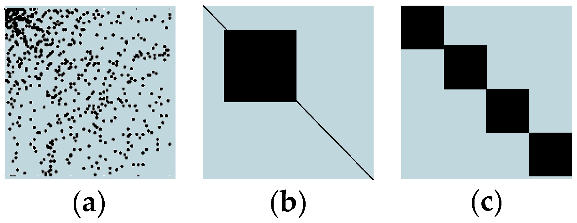
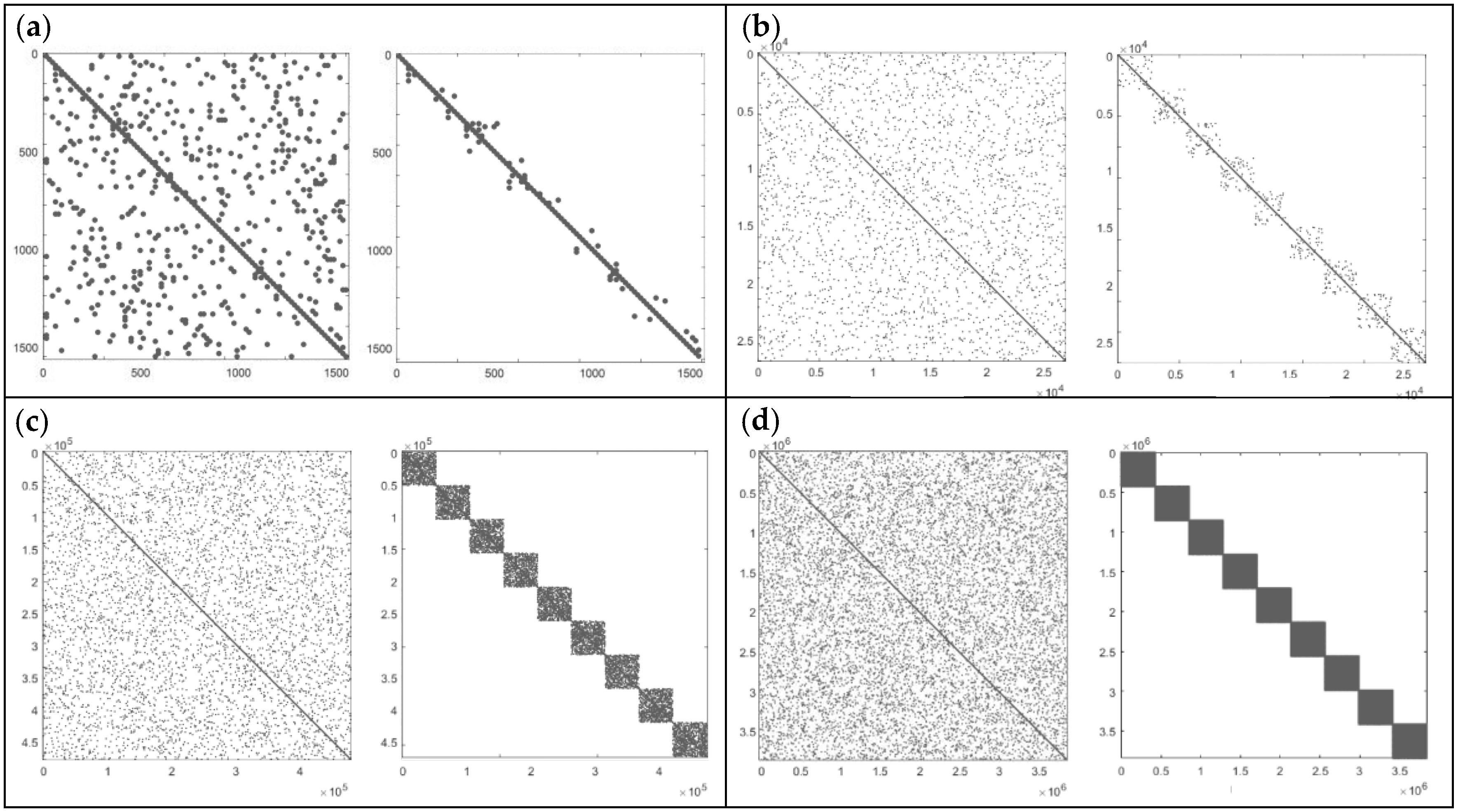
4.3.3. Comparison of Distribution Change After Matrix Preconditioning

Due to the characteristics of sparse matrices, where most elements are zero and the distribution of non-zero elements is highly scattered, this poses a significant challenge to matrix solution efficiency. The G-Pre used in this section optimizes the matrix structure by employing a graph theory preconditioner, which adjusts the distribution of non-zero elements to concentrate them, thereby facilitating the solving operation. The changes in the distribution of the matrix before and after G-Pre preconditioning are illustrated in Figure 6.

From the changes observed in different matrices, it can be seen that chunk map reordering made the non-zero elements appear in blocks of consecutive rows, with similar densities across these rows. This significantly improved the spatial locality of memory access patterns and promoted a balanced load distribution during parallel computation across different blocks. Particularly in Matrix 4, the reordered elements were closer to those of a dense matrix, which is advantageous for computational solving.

However, in Matrices 1, 2, and 3, the preconditioning effect was less satisfactory. In the first two matrices, the distribution of elements after preconditioning remained relatively scattered, which hindered the improvements to the solution efficiency. This observation highlights that the current G-Pre preconditioning algorithm still has areas that require enhancement. Specifically, efficiently preconditioning small-sized matrices to achieve optimal results remains a key area for future improvement.

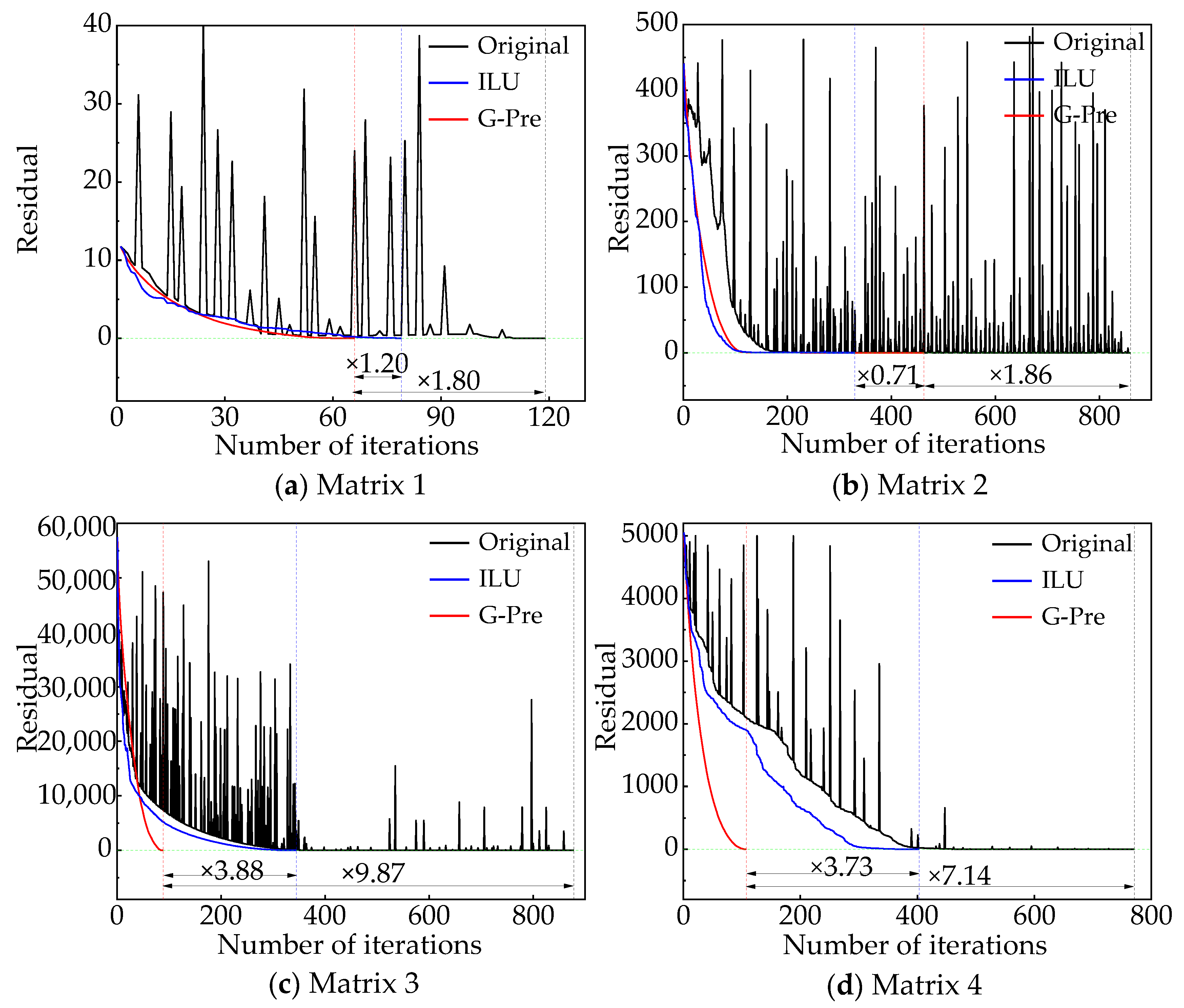
4.3.4. Comparison of the Convergence Performance in the Matrix Solving Process

Due to the prevalence of sparse matrices in practical applications, which significantly affect the stability of the matrix solving process, oscillations often occur during iterative solving. Specifically, the residual values during iteration do not maintain a monotonically decreasing trend and may exhibit occasional spikes or inverse biases. The presence of such oscillations indicates poor disturbance resistance in the linear system, leading to larger responses to potential perturbations, thereby impacting the efficiency and stability of the linear system.

Optimizing the matrix condition number and structure using preconditioning can mitigate these oscillations during the iterative process. Both the convergence performance and stability during the solution process are illustrated in Figure 7 for numerical experiments involving four matrices. It is important to note that for a better comparison during the iteration process, the shown solution iteration processes do not necessarily correspond to those with the fastest solving times and thus may not directly reflect the solving times discussed in the previous section.

Without preconditioning, the residuals in the matrix iteration process frequently exhibit abnormal fluctuations, resulting in extremely large values—an indication of oscillation. This makes the matrix iteration convergence process less stable. The root cause of this oscillation is the high condition number of the matrix, i.e., the matrix is “ill-conditioned”, making it highly sensitive to small perturbations in input data, which amplifies numerical errors during the solving process, affecting both efficiency and convergence performance.

After applying G-Pre and ILU preconditioning, the matrix condition numbers were reduced, and the iteration process became more stable, leading to an improved convergence performance. As shown in the condition number comparisons, G-Pre further reduced the number of iterations by factors of 2.4 and 5.2, respectively. Additionally, when combined with the solving time comparisons, it was evident that G-Pre did not show a significant advantage in Matrices 1 and 2. However, the reduction in the number of iterations also led to a decrease in solving time. It should be noted that the speedup ratio in terms of the number of iterations did not directly translate to the speedup ratio in solving time. This is because the number of iterations in the solving process is not linearly related to time; fewer iterations merely indicate a better convergence performance.

4.3.5. Comparison of the Accuracy of Matrix Solving Results

Both the result accuracy and solution efficiency are crucial metrics in matrix solving. The accuracy of the results determines whether the final simulation outcomes can accurately reflect real-world situations. It is essential for a solver to produce accurate results while maintaining high solution efficiency, which is vital for the comprehensive evaluation of the solution process. To further investigate whether the G-Pre solving process affects the matrix results, this section compares its solving results with the original results. The error analysis, which is presented in Figure 8, shows that the errors in the results obtained from G-Pre remained at around 1%. This indicates that using G-Pre has minimal impact on the matrix results, thereby validating the feasibility and effectiveness of the G-Pre algorithm. The low error rate demonstrates that G-Pre not only achieved a high solution efficiency but also maintained a high level of accuracy. These findings reinforce the suitability of G-Pre for practical applications where both precision and performance are critical. However, it is also easy to see from Figure 8 that the error rate of the results of the small-scale Matrix 3 was higher than that of the large-scale Matrix 4. This is contrary to the difference in dimensions between Matrix 3 and Matrix 4. To analyze why the difference occurred, it can be compared with the iterative convergence process of the matrices in Figure 7. As can be seen in Figure 7, the residuals at the beginning of the iteration for Matrix 3 were much larger than the initial residuals for Matrix 4. This was due to the difference between the initial solution determined at the beginning stage of the iterative method and the actual solution, whereby the initial solution assumed for Matrix 3 had a larger error from the actual solution. This also affected the greater error in the approximate solution that was eventually obtained, resulting in a different value of the residuals of the two matrices from the convergence bounds when the convergence bounds were reached, which, in turn, made the error in the results of Matrix 3 greater.

4.4. Application Testing

In order to evaluate the effectiveness of the proposed G-Pre preconditioning algorithm in practical applications, a total of four static analysis models were selected in this paper; their detailed information is shown in

Table 3. Model information.

Model	Model File Size	Nodes	Matrix Dimension	Non-Zero Elements	Matrix File Size
Model 1	6 KB	60	180	6298	190 KB
Model 2	965 KB	10,863	32,589	1,996,613	67.4 MB
Model 3	20 MB	463,874	532,146	38,501,924	1.34 GB
Model 4	205 MB	3,648,656	4,824,972	371,365,956	13.6 GB

. Figure 9 shows a visual schematic of each model, where the red arrows indicate the forces applied to the finite element model, and the black arrows indicate the fixed constraints of the model. It should be noted that while the scale of each model only represents the size of its basic constituent finite element mesh, there were also encrypted meshes within the different models that were smaller in size. A brief description of the different models is given below. Model 1 represents a simple cantilever beam with one end fixed and the other end subjected to a static load. Model 2 depicts a perforated plate structure with one end fixed and the other end subjected to a static tensile force aligned with the surface of the plate. Model 3 is a simple printed circuit board with two sides and a fixed through-hole; there is a static force acting on one corner of the board. Model 4 is a BGA circuit board with the bottom edge, holes, and two sides held stationary, and a static force acting on one side of the board.

A comparison of solution times for the corresponding models is shown in

Table 4. Comparison of solution times for finite element simulation models.

Model	Original	ILU	G-Pre
Model 1	0.0692	0.0227	0.0396
Model 2	0.327	0.242	0.155
Model 3	15.2	4.56	1.45
Model 4	64.8	49.6	28.1

. It can be observed that the characteristics of the G-Pre preconditioning algorithm were consistent with those analyzed in previous matrix experiments within the real simulation model. Firstly, it was evident that the G-Pre preconditioning algorithm improved the efficiency of solving the models. Furthermore, the optimization effect of the G-Pre preconditioning algorithm became increasingly prominent as the model size increased. Specifically, for Models 3 and 4, improvements of 1.29- and 2.41-fold, respectively, were achieved compared to ILU preconditioning. However, for small-scale simulation models, such as Model 1, the optimization effect brought about by the G-Pre preconditioning algorithm was not as significant. In fact, there was even a slight deterioration in solution efficiency when compared to ILU preconditioning. This suggests that the limitations of the G-Pre preconditioning algorithm in handling small-scale models may become more apparent in practical applications, highlighting an area for improvement in future research.

5. Conclusions

Traditionally, the preconditioning of solution algorithms for linear systems of equations discretized using the finite element method has relied on the conventional ILU factorization method. This approach often results in unsatisfactory preconditioning effects, accompanied by increased computational costs and challenges in achieving parallelism. To address these issues, we propose a preconditioning algorithm named G-Pre, which is based on graph–theoretic methods, to enhance the efficiency of solving linear systems of equations. In the proposed method, a combination of graph partitioning, graph reordering, and ILU factorization was employed to concentrate the non-zero elements of the coefficient matrix, thereby improving data access efficiency and facilitating parallelism through matrix partitioning. Numerical experiments were conducted using test matrices, and an actual finite element model was utilized for further testing. The results demonstrated that the G-Pre preconditioning algorithm proposed in this paper can improve the condition number optimization by 2.6-fold compared with that of ILU preconditioning; the solution efficiency can be improved 2.1- and 4.3-fold compared with ILU preconditioning and direct solvers. In terms of iterative convergence performance, the number of iterations can be reduced by an average of 30.8% compared with ILU preconditioning. Meanwhile, the resultant error can be maintained at 1%. It has been proven that the G-Pre preconditioning algorithm can improve the convergence performance of the solver and shorten the solution time.

However, the current G-Pre preconditioning algorithm still has some shortcomings. First, there is no clear optimization effect of the algorithm in the small-scale matrix solving process, and in some situations, it is not as good as ILU preconditioning. Secondly, the initial solution of the algorithm needs to be further optimized so that the initial residuals are too large, which affects the iterative convergence process and the error of the results. Finally, the possibility of combining more solution algorithms and preconditioning algorithms should be considered to further broaden the applicability of the G-Pre preconditioning algorithm. In future work, further refinement is planned to address the shortcomings of the current algorithm in order to improve its performance. First, the performance of the G-Pre preconditioning algorithm in small-scale matrices needs to be improved, and the introduction of an adaptive algorithm can be considered to reduce the time cost of the graph algorithm in small-scale matrices. In addition, the setting of the initial solution needs to be further optimized to reduce the impact on iterative convergence. Meanwhile, a supervised optimization procedure can also be considered to judge the quality of the initial solution and to reset it if it does not meet the requirements. Finally, introducing more advanced techniques such as a graph neural network in the preconditioning algorithm can also further improve its efficiency. Further research will be carried out in future work to make continuous efforts to realize an efficient G-Pre preconditioning algorithm.

References

1. Tan, X.; Chen, T. A Mixed Finite Element Approach for A Variational-Hemivariational Inequality of Incompressible Bingham Fluids. J. Sci. Comput. 2025, 103, 36. [Google Scholar] [CrossRef]
2. Caucao, S.; Gatica, G.N.; Gatica, L.F. A posteriori error analysis of a mixed finite element method for the stationary convective Brinkman–Forchheimer problem. Appl. Numer. Math. 2025, 211, 158–178. [Google Scholar] [CrossRef]
3. Rahman, H.A.; Ghani, J.A.; Rasani, M.R.M.; Mahmood, W.M.F.W.; Yaaqob, S.; Abd Aziz, M.S. Application of Finite Element Analysis and Computational Fluid Dynamics in Machining AISI 4340 Steel. Tribol. Int. 2025, 207, 110616. [Google Scholar] [CrossRef]
4. Deng, G.; Chen, L.; Zhu, S.; Deng, G.; Chen, L.; Zhu, S.; Yun, Z.; Fan, H.; Chen, Y.; Hou, X.; et al. Preparation and quasi-static compressive behavior of fiber-reinforced truncated conical shells. Thin-Walled Struct. 2025, 210, 113035. [Google Scholar] [CrossRef]
5. Özdemir, A.M. Experimental evaluation and 3D finite element simulation of creep behaviour of SBS modified asphalt mixture. Constr. Build. Mater. 2025, 460, 139821. [Google Scholar] [CrossRef]
6. Wu, D.; Xue, Z.; Ni, Z.; Li, Y.; Chen, Z.; Zhu, X.; Xu, Y.; Lu, P.; Zhang, L.; He, J. Deformation Mechanisms of Nanoporous Oxide Glasses: Indentations and Finite Element Simulation. Acta Mater. 2025, 287, 120779. [Google Scholar] [CrossRef]
7. Jellicoe, M.; Yang, Y.; Stokes, W.; Simmons, M.; Yang, L.; Foster, S.; Aslam, Z.; Cohen, J.; Rashid, A.; Nelson, A.L. Continuous Flow Synthesis of Copper Oxide Nanoparticles Enabling Rapid Screening of Synthesis-Structure-Property Relationships. Small 2025, 21, 2403529. [Google Scholar] [CrossRef]
8. Lu, Y.; Hong, W.; Wu, W.; Zhang, J.; Li, S.; Xu, B.; Wei, K.; Liu, S. The impact of temperature regulation measures on the thermodynamic characteristics of bee colonies based on finite element simulation. Biosyst. Eng. 2025, 250, 306–316. [Google Scholar] [CrossRef]
9. Lee, J.S.; Ramos-Sebastian, A.; Yu, C.; Kim, S.H. A multi-focused electrospinning system with optimized multi-ring electrode arrays for the wasteless parallel fabrication of centimeter-scale 2D multilayer electrospun structures. Mater. Today Adv. 2025, 25, 100563. [Google Scholar] [CrossRef]
10. Fialko, S. Parallel Finite Element Solver for Multi-Core Computers with Shared Memory. Comput. Math. Appl. 2021, 94, 1–14. [Google Scholar] [CrossRef]
11. Wang, Y.; Wang, S.; Cai, Y.; Wang, G.; Li, G. Fully Parallel and Pipelined Sparse Direct Solver for Large Symmetric Indefinite Finite Element Problems. Comput. Math. Appl. 2024, 175, 447–469. [Google Scholar] [CrossRef]
12. Zheng, S.; Xu, R. ZjuMatrix: C++ Vector and Matrix Class Library for Finite Element Method. SoftwareX 2024, 27, 101825. [Google Scholar] [CrossRef]
13. Wang, Y.; Luo, S.; Gu, J.; Zhang, Y. Efficient Blocked Symmetric Compressed Sparse Column Method for Finite Element Analysis. Front. Mech. Eng. 2025, 20, 5. [Google Scholar] [CrossRef]
14. Jang, Y.; Grigori, L.; Martin, E.; Content, C. Randomized Flexible GMRES with Deflated Restarting. Numer. Algorithms 2024, 98, 431–465. [Google Scholar] [CrossRef]
15. Thomas, S.; Carson, E.; Rozložník, M.; Carr, A.; Świrydowicz, K. Iterated Gauss–Seidel GMRES. SIAM J. Sci. Comput. 2024, 46, S254–S279. [Google Scholar] [CrossRef]
16. Rump, S.M.; Ogita, T. Verified Error Bounds for Matrix Decompositions. SIAM J. Matrix Anal. Appl. 2024, 45, 2155–2183. [Google Scholar] [CrossRef]
17. Mejia-Domenzain, L.; Chen, J.; Lourenco, C.; Moreno-Centeno, E.; Davis, T.A. Algorithm 1050: SPEX Cholesky, LDL, and Backslash for Exactly Solving Sparse Linear Systems. ACM Trans. Math. Softw. 2025, 50, 1–29. [Google Scholar] [CrossRef]
18. Dai, S.; Zhao, D.; Wang, S.; Li, K.; Jahandari, H. Three-Dimensional Magnetotelluric Modeling in A Mixed Space-Wavenumber Domain. Geophysics 2022, 87, E205–E217. [Google Scholar] [CrossRef]
19. Meijerink, J.A.; Van, D.V. An Iterative Solution Method for Linear Systems of Which the Coefficient Matrix is a Symmetric M-Matrix. Math. Comput. 1977, 31, 148–162. [Google Scholar] [CrossRef]
20. Cerdán, J.; Marín, J.; Mas, J. A two-level ILU preconditioner for electromagnetic applications. J. Comput. Appl. Math. 2017, 309, 371–382. [Google Scholar] [CrossRef]
21. Li, W.; Chen, Z.; Ewing, R.E.; Huan, G.; Li, B. Comparison of the GMRES and ORTHOMIN for the black oil model in porous media. Int. J. Numer. Methods Fluids 2005, 48, 501–519. [Google Scholar] [CrossRef]
22. Saad, Y.; Schultz, M.H. GMRES: A generalized minimal residual algorithm for solving nonsymmetric linear systems. SIAM J. Sci. Statist. Comput. 1986, 7, 856–869. [Google Scholar] [CrossRef]
23. Zhang, X.F.; Xiao, M.L.; He, Z.H. Orthogonal Block Kaczmarz Inner-Iteration Preconditioned Flexible GMRES Method for Large-Scale Linear Systems. Appl. Math. Lett. 2025, 166, 109529. [Google Scholar] [CrossRef]
24. Wang, J.; Zuo, S.; Zhao, X.; Tian, M.; Lin, Z.; Zhang, Y. A Parallel Direct Finite Element Solver Empowered by Machine Learning for Solving Large-Scale Electromagnetic Problems. IEEE Trans. Antennas Propag. 2025, 73, 2690–2695. [Google Scholar] [CrossRef]
25. Hu, X.; Lin, J. Solving Graph Laplacians via Multilevel Sparsifiers. SIAM J. Sci. Comput. 2024, 46, S378–S400. [Google Scholar] [CrossRef]
26. Bioli, I.; Kressner, D.; Robol, L. Preconditioned Low-Rank Riemannian Optimization for Symmetric Positive Definite Linear Matrix Equations. SIAM J. Sci. Comput. 2025, 47, A1091–A1116. [Google Scholar] [CrossRef]
27. Luo, Z.; Zhong, Y.; Wu, F. A review of preprocessing techniques in the solution of sparse systems of linear equations. Comput. Eng. Sci. 2010, 32, 89–93. [Google Scholar]
28. Saad, Y. Iterative Methods for Sparse Linear Systems, 2nd ed.; SIAM: Philadelphia, PA, USA, 2003; pp. 326–330. [Google Scholar]
29. Benson, M.W.; Paul, O.; Frederickson. Iterative Solution of Large Sparse Linear Systems Arising in Certain Multidimensional Approximation Problems. Util. Math. 1982, 22, 127–140. [Google Scholar]
30. Wang, Z.D.; Huang, T.Z. Comparison Results Between Jacobi and Other Iterative Methods. J. Comput. Appl. Math. 2004, 169, 45–51. [Google Scholar] [CrossRef]
31. Lynn, M.S. On the Round-Off Error in the Method of Successive Over Relaxation. Math. Comput. 1964, 18, 36–49. [Google Scholar] [CrossRef]
32. Xu, T.; Li, R.P.; Osei, K.D. A two-level GPU-accelerated incomplete LU preconditioner for general sparse linear systems. Int. J. High Perform. Comput. Appl. 2025, 39, 10943420251319334. [Google Scholar] [CrossRef]
33. Van Der Vorst, H.A. Iterative Krylov Methods for Large Linear Systems; Cambridge University Press: Cambridge, UK, 2003; pp. 183–185. [Google Scholar]
34. Saad, Y. ILUT: A dual threshold incomplete LU factorization. Numer. Linear Algebra Appl. 1994, 1, 387–402. [Google Scholar] [CrossRef]
35. Li, N.; Saad, Y.; Chow, E. Crout versions of ILU for general sparse matrices. SIAM J. Sci. Comput. 2003, 25, 716–728. [Google Scholar] [CrossRef]
36. Suzuki, K.; Fukaya, T.; Iwashita, T. A novel ILU preconditioning method with a block structure suitable for SIMD vectorization. J. Comput. Appl. Math. 2023, 419, 114687. [Google Scholar] [CrossRef]
37. Osei-Kuffuor, D.; Li, R.; Saad, Y. Matrix reordering using multilevel graph coarsening for ILU preconditioning. SIAM J. Sci. Comput. 2015, 37, A391–A419. [Google Scholar] [CrossRef]
38. Zheng, Q.; Xi, Y.; Saad, Y. Multicolor low-rank preconditioner for general sparse linear systems. Numer. Linear Algebra Appl. 2020, 27, e2316. [Google Scholar] [CrossRef]
39. Wang, C.; Liu, Q.; Wang, Z.; Cheng, X. A review of power battery cooling technologies. Renew. Sustain. Energy Rev. 2025, 213, 115494. [Google Scholar] [CrossRef]
40. Qu, Z.; Xie, Y.; Zhao, T.; Xu, W.; He, Y.; Xu, Y.; Sun, H.; You, T.; Han, G.; Hao, Y.; et al. Extremely Low Thermal Resistance of β-Ga2O3 MOSFETs by Co-integrated Design of Substrate Engineering and Device Packaging. ACS Appl. Mater. Interfaces. 2024, 16, 57816–57823. [Google Scholar] [CrossRef]
41. Lin, Y.; Cao, L.; Tan, Z.; Tan, W. Impact of Dufour and Soret effects on heat and mass transfer of Marangoni flow in the boundary layer over a rotating disk. Int. Commun. Heat Mass Transf. 2024, 152, 107287. [Google Scholar] [CrossRef]
42. Ma, C.W.; Yu, S.H.; Fang, J.K.; Yang, P.F.; Chang, H.C. The physical improvement of copper deposition uniformity with the simulation models. J. Electroanal. Chem. 2023, 948, 117790. [Google Scholar] [CrossRef]
43. Majeed, A.H.; Mahmood, R.; Liu, D. Finite element simulations of double diffusion in a staggered cavity filled with a power-law fluid. Phys. Fluids. 2024, 36, 3. [Google Scholar] [CrossRef]
44. Yu, B.; Li, Y.; Liu, J. A Positivity-Preserving and Robust Fast Solver for Time Fractional Convection-Diffusion Problems. J. Sci. Comput. 2024, 98, 59. [Google Scholar] [CrossRef]
45. Feron, J.; Latteur, P.; Pacheco de Almeida, J. Static Modal Analysis: A Review of Static Structural Analysis Methods Through a New Modal Paradigm. Arch. Comput. Methods Eng. 2024, 31, 3409–3440. [Google Scholar] [CrossRef]
46. Oliker, L.; Li, X.; Husbands, P.; Biswas, R. Effects of Ordering Strategies and Programming Paradigms on Sparse Matrix Computations. Siam Rev. 2002, 44, 373–393. [Google Scholar] [CrossRef]
47. Edalatpour, V.; Hezari, D.; Salkuyeh, D.K. A Generalization of the Gauss–Seidel Iteration Method for Solving Absolute Value Equations. Appl. Math. Comput. 2017, 293, 156–167. [Google Scholar] [CrossRef]
48. De, S.B.; De, M.B. The QR Decomposition and the Singular Value Decomposition in the Symmetrized Max-Plus Algebra Revisited. Siam Rev. 2002, 44, 417–454. [Google Scholar]
49. Chen, Q.X.; Huang, G.X.; Zhang, M.Y. Preconditioned BiCGSTAB and BiCRSTAB methods for solving the Sylvester tensor equation. Appl. Math. Comput. 2024, 466, 128469. [Google Scholar] [CrossRef]
50. Wu, J.; Wang, Z.; Li, X. Efficient Solution and Parallel Computing of Sparse Systems of Linear Equations; Hunan Science and Technology Press: Changsha, China, 2004. [Google Scholar]
51. D’Azevedo, E.F.; Forsyth, P.A.; Tang, W.-P. Towards a cost effective ILU preconditioner with high level fill. BIT Numer. Math. 1992, 32, 442–463. [Google Scholar] [CrossRef]
52. D’Azevedo, E.F.; Forsyth, P.A.; Tang, W.-P. Ordering methods for preconditioned conjugate gradient methods applied to unstructured grid problems. SIAM J. Matrix Anal. Appl. 1992, 13, 944–961. [Google Scholar] [CrossRef]
53. Karypis, G.; Kumar, V. Parallel multilevel k-way partitioning scheme for irregular graphs. In Proceedings of the 1996 ACM/IEEE Conference on Supercomputing, Pittsburgh, PA, USA, 1 January 1996; IEEE: Washington, DC, USA; ACM: New York, NY, USA, 1996; p. 35-es. [Google Scholar]
54. Grama, A. An Introduction to Parallel Computing: Design and Analysis of Algorithms, 2/e; Pearson Education India: Delhi, India, 2008; pp. 125–133. [Google Scholar]
55. Karypis, G.; Kumar, V. A fast and high quality multilevel scheme for partitioning irregular graphs. SIAM J. Sci. Comput. 1998, 20, 359–392. [Google Scholar] [CrossRef]
Figure 1. Schematic diagram of the LU factorization process of A.
Applsci 15 05130 g001
Figure 2. Schematic of SpMV operation for sparse matrices.
Applsci 15 05130 g002
Figure 3. Graph reordering schematic.
Applsci 15 05130 g003
Figure 4. Schematic diagram for dividing and rearranging matrices. (a) Original matrix; (b) full graph rearrangement; (c) graph division and rearrangement.
Applsci 15 05130 g004
Figure 5. Comparison of solution times for different models with no preconditioning, ILU preconditioning, and G-Pre preconditioning. (ad) Matrices 1–4.
Applsci 15 05130 g005
Figure 6. Comparison of the distribution of matrix plots before/after G-Pre preconditioning. (ad) Matrices 1-4. The left side is the distribution of matrix plots before G-Pre preconditioning, and the right side is the distribution of matrix plots after G-Pre preconditioning.
Applsci 15 05130 g006
Figure 7. Comparison of iterative processes for different matrices under different preconditioning conditions.
Applsci 15 05130 g007
Figure 8. Comparison of the accuracy of the results of solving different matrices.
Applsci 15 05130 g008
Figure 9. A visualization of the different models.
Applsci 15 05130 g009