Managing Operational Efficiency and Reducing Aircraft Downtime by Optimization of Aircraft On-Ground (AOG) Processes for Air Operator

Abstract

This research aims to identify patterns and root causes of aircraft downtimes by comparing various forecasting models used in the aviation industry to prevent AOG events effectively. At its heart, this study explores innovative forecasting models using time series analysis, time series modeling and binary classification to predict spare part usage, reduce downtime, and tackle the complexities of managing inventory for diverse aircraft fleets. By analyzing both data and insights shared by aviation industry experts, the research offers a practical roadmap for enhancing supply chain efficiency and reducing Mean Time Between Failures (MTBF). The thesis emphasizes how real-time data integration and hybrid forecasting approaches can transform operations, helping airlines keep spare parts available when and where they are needed most. It also shows how precise forecasting is not just about saving costs, it is about boosting customer satisfaction and staying competitive in an ever-demanding industry. In addition to data-driven insights, this research provides actionable recommendations, such as embracing predictive maintenance strategies and streamlining logistics. These steps aim to ensure smoother operations, fewer disruptions, and more reliable service for passengers and operators alike.

1. Introduction

In the high-stakes, precision-driven world of commercial aviation, operational efficiency and aircraft availability are not just performance metrics, they are strategic imperatives. Every minute an aircraft is grounded due to technical issues, known as an Aircraft On-Ground (AOG) event, translates into substantial economic loss, operational disruption, and diminished customer satisfaction. With airlines navigating increasingly complex fleet compositions, global supply chains, and fluctuating market demands, the urgency to predict, prevent, and manage AOG events has never been greater. At the center of this issue lies the sophistication involved in forecasting spare part requirements, planning with suppliers, and optimizing maintenance practices to minimize surprises in downtimes. Traditional reactive or preventive maintenance strategies based on historical patterns or fixed intervals do not suffice in a digital economy where real-time data, AI, and machine learning offer significantly more advanced and accurate tools for decision-making. Predictive maintenance, supported by advanced predictive models, is a revolutionary strategy that allows airlines to predict failures, ensure on time part availability, and keep fleets flying. This research examines the strategic and operational characteristics of AOG management, taking SmartLynx Airlines as a research base. It explores how sophisticated prediction techniques such as ARIMA, Holt–Winters exponential smoothing, and Logistic Regression are supplemented by live operational data to reduce Mean Time Between Failures (MTBF) and enhance maintenance scheduling and inventory management.

By uniting quantitative data analysis and qualitative industry insight, the study aims to find actionable pathways that not only mitigate AOG events but also provide quantifiable financial and operational benefits. Through the integration of statistical modeling with real-world experience of airline logisticians and engineers, this paper presents a holistic model for AOG process optimization. It tries to address the gap between theoretical abstract forecasting models and real-world aviation logistics, proposing solutions that are scalable while maintaining maintenance strategies aligned with business objectives in a competitive and regulated global business.

2. Literature Review

The airline industry is pivotal in today’s global economy, driving economic growth and development. Expanding the travel and tourism sectors underscores air transport’s significance as a cornerstone of this industry [1]. Additionally, aviation contributes approximately 3.5% of global GDP and supports over three billion air passengers annually, positioning air transport as one of the most influential industries [2].

Nevertheless, numerous challenges face the substantial growth of the aviation business. One of the critical challenges airlines faces is forecasting the spare parts needed for unexpected maintenance. Accurate forecasting methods are vital to minimize Aircraft On-Ground (AOG) events [3]. Ensuring the timely availability of required parts prevents delays and operational disruptions, ultimately preserving efficiency and reliability in airline services. In aviation, the term Aircraft On-Ground (AOG) refers to situations where technical issues prevent an aircraft from completing its flight [4]. The International Air Transport Association (IATA) categorizes airline spare parts into three primary types: rotable, repairable, and expendable. Rotable parts typically have a low scrap rate, while repairable parts require careful planning to avoid excessive waste [5]. Expendable parts, in contrast, are used only once before being discarded. Life-limited parts are designed for a specific operational cycle, while consumable parts are entirely disposed of after use.

Technical failures often necessitate the replacement of critical components, causing grounded aircraft and operational disruptions. Frequent AOG situations impose substantial costs and damage an airline’s reputation. The diverse aircraft types in a company’s fleet sourced from multiple manufacturers further complicate inventory management and forecasting processes. The high costs associated with stockouts underscore the need for precise forecasting methods to optimize material management and ordering procedures.

Numerous forecasting methods address the challenge of predicting spare part demand in aviation, yet their effectiveness varies across different parts and demand patterns [6]. Among these, time series analysis, time series modeling, and binary classification methods return to service are reliable tools for forecasting airline spare parts. These methods can significantly reduce operational costs, benefiting airlines and their customers [7]. Despite the well-documented importance of forecasting AOG events, the academic literature rarely explores advanced or real-time strategies tailored to these scenarios. This study focuses on innovative solutions like real-time sensor analytics, IoT-enabled data collection, and rapid anomaly detection algorithms. For example, live data feeds from aircraft systems can generate near-instant alerts for emerging technical issues, while machine learning algorithms can analyze failure patterns to expedite maintenance decisions. When tested in select airline operations, these methods have demonstrated their potential to detect anomalies early and facilitate proactive repairs. By integrating these advanced tools, this research contributes to a more robust understanding of AOG mitigation strategies and offers practical approaches for improving operational efficiency in the aviation industry.

Airline operations management is a complex affair that involves coordination with various actors. The most critical link in a chain is the Airline Operations Manager (AOM), who is responsible for the daily operations of large fleets and often checks 40–50 flights an hour. AOMs are dealing with irregular operations caused by adverse weather, Air Traffic Control (ATC) delays, and unexpected maintenance, which is why they exist in the first place. Their job is not only to take the plane but also to make crucial decisions against delays, cancelations, vehicle switches, and dispatching of reserved crews; all of these will minimize disturbances and ensure the successful running of the operations.

In instances where irregular operations affect over 10% of the daily flights, enhanced AOM performance can lead to significant economic gains. Operations Research (OR) methods, such as mathematical programming, successfully assist AOMs in recovering from disturbances. These algorithms can create a solution that can address specific real-time challenges, focusing on such factors as aircraft utilization and minimizing downtime delays. Nevertheless, despite these optimization tools’ potential, AOMs often do not have the necessary support systems to assess the algorithm outputs in their specific contexts. Creating those systems aims to impart precision capability to AOMs so they can make decisions that match the actual data. On top of that, malfunctions in some departments can create Aircraft On-Ground (AOG) anomalies. For instance, maintenance delivery of parts or a staffing issue can lead to the aircraft taking longer to be repaired. This, in turn, would complicate the recovery work when the problems are being addressed. AOG events can cause broader operational difficulties, such as flight delays and lower customer satisfaction. To conclude, designing efficient AOG management solutions is a top priority for the aviation industry.

The past few years have seen the aviation industry experience a technological shift towards data-driven maintenance, with predictive maintenance being a highlight. Studies such as [8,9] have explored the application of AI and data analytics in anomaly detection in aircraft systems. But these works generally have a tendency to concentrate on system-level diagnostics, typically without wider integration with supply chain activities and spare parts forecasting—a domain of enormous strategic significance for effective AOG (Aircraft On-Ground) management.

Also, while such products as Skywise by Airbus and Prognos by AFI KLM [10] have demonstrated their effectiveness at applying real-time data for the monitoring of components, they tend to focus mostly on technical alarms rather than on predicting spare parts demand or on aligning maintenance strategy with procurement cycles. This disconnection is also experienced in the academic literature, where methods like ARIMA and LSTM have been applied to forecast equipment failure but rarely connected to real fleet-level logistics, cost savings, or spare part optimization.

Works by [11,12] have raised the logistical challenges of predictive maintenance but with a tendency to treat them in isolation from operations data like MTBF, frequency of AOG events, and delay times. The novelty of this study lies in the integrated combination of real-time airline data, state-of-the-art prediction models, and operational impact analyses. Through the combination of statistical techniques such as ARIMA, Holt–Winters, and Logistic Regression with real-time SmartLynx operational data, this research provides not only predictive data but also prescriptive recommendations for inventory and downtime management.

This paper also addresses a critical literature need by analyzing the economic return on predictive maintenance and quantifying the effects of how accurate forecasting can eliminate AOG events, optimize part availability, and minimize fleet disruption. The methodology used goes beyond theoretical modeling—it includes real feedback from airline logisticians and engineers and compares findings over multiple aircraft types. Therefore, this research makes a distinct contribution by bringing together predictive modeling, airline maintenance planning, and inventory forecasting under one holistic AOG mitigation framework. It extends the current body of literature by introducing a scalable, data-tested roadmap that is implementable across various airline operating models.

3. Framework of Forecasting AOG Models in Aviation

3.1. Overview and Definition of AOG in Aviation Industry

AOG refers to an airplane that cannot fly due to technical issues, often requiring urgent maintenance, parts replacement, or repair. In other words, it means a loss of operational capacity and can have significant financial implications for airlines and associated stakeholders. According to IATA, delays and disruptions caused by AOG events can lead to substantial operational costs, impacting revenue and customer satisfaction [13].

The fault rectification flowchart (Figure 1), designed for maintenance failures, is an overview of the course of action relating to an aircraft with technical problems. The first part of the chart illustrates the situation when an issue occurs and good-conditioned spare parts are available. Local rectification follows for a particular scenario. The second part of the flowchart describes the step-by-step actions that shall be taken to return the aircraft to service in case of AOG. The initial phase involves identifying that the fault cannot be rectified locally. At this stage, the problem is confirmed in the MEL Defect category, which involves the Integrated Operations Control Centre (IOCC) receiving the immediate report. The IOCC controls and secures high-impact aircraft operations and regulatory compliance. The primary aim of the IOCC is event response coordination, which involves the team making up the immediate report, as well as urgently deciding which operating aircraft should be alive and ensuring compliance with the established safety standards. The next step includes the Analysis of Deviation along with the decision-making capability. This stage entailed the engineering teams performing inspections and tests to identify the fault, utilizing diagnostic tools and historical data. This step is a significant factor that detects the root cause of the problem and the goals, thereby defining the solution with the help of safety and regulatory authorities.

The following phase of the process is rectifying possibilities by the team through intensive troubleshooting work. This phase is often a circular process with the involvement of suppliers or maintenance organizations from the “outside”. Troubleshooting in the industry is required to keep in check the air traffic technicians; thus, Civil Aviation Authorities standards rank as the topmost consideration. The long-awaited resolution of the difficulties follows with the definition of the Rectification Options executed by the Maintenance Control Center (MCC). At this stage, the emphasis is on the prompt availability of parts, resources, and skilled craft people.

This phase requires strictly following the guidelines on maintenance and documentation as mandated by aviation regulatory bodies. The last phase, which involves the preparation of the follow-up documentation, monitors such actions to guarantee that Airworthiness Certificates are issued. This makes it a legal requirement that everybody follows the aviation rules, which include keeping the operation safe and certifying it.

• AOG Management Procedures

According to the guidelines from the ICAO, aviation companies ought to have comprehensive reporting systems in place so that AOG events can be documented in real-time data [14]. In the event of an AOG detection, airlines start a phased response process, which usually includes the following actions:

-

Issue Assessment;

-

Parts Procurement;

-

Repair and Maintenance;

-

Quality Control;

-

Return to Service.

The primary stakeholders are to be informed after the quality assurance check is passed and the aircraft returns to service.

• How Is AOG Managed with Technology?

The arising technological era has initiated a new era for the management of AOG. The use of real-time monitoring systems such as the Vehicle Health Monitoring System (VHMS) that enable airlines to apprehend potential technical ahead of their evolution to an AOG event is amongst the benefits associated with such technologies. With these systems, airlines can utilize data analysis and machine learning algorithms to study the performance of their planes and find the need for maintenance, which will significantly decrease AOG scenarios [15]. In addition, embedding mobile technology, among other things, will allow maintenance teams to be immediately alerted to AOG issues and act quickly. As an illustration, a study by the National Institute of Aerospace (NIA) showed that mobile applications for maintenance reporting and tracking can lower AOG resolution times by up to 30% [16].

• Interpretation of Case Studies

An example of a successful case in AOG management is Lufthansa Technik, which devised a comprehensive AOG response plan. They found that the utilization of a proactive approach to maintenance helped them reduce their AOG bills. With predictive analytics, they could predict potential failures and be prepared before they occur [17]. In the same dimension, Delta Air Lines demonstrated how they resolved an AOG event through a creative logistics solution. By establishing a chain of warehouses in key locations, Delta reduced AOG times by ensuring that necessary parts were promptly available through a short supply chain [18].

• AOG Events and Financial Implications

The AOG events are an incessant financial challenge for airlines, affecting their direct expenses and related demand. According to the Aviation Outlook Newsletter [19], AOG-related costs can range from EUR 10,000 to EUR 150,000/h, mainly depending on the airline’s operational scale, aircraft type, and the nature of the event. Moreover, such expenses are usually accompanied by the urgency of the need for spare parts, additional maintenance work, and compensating affected passengers (

Table 1. Financial impacts and cost breakdown of AOG events in aviation industry [19].

Financial Factor	Estimated Cost Range (EUR) per Day	Factor Metrics
Hourly AOG Cost (per hour)	EUR 10,000–EUR 150,000	Costs increase based on aircraft type (e.g., narrow-body vs. wide-body) and route profitability.
Expedited Parts Costs	EUR 5000–EUR 60,000	Costs depend on the part’s criticality, availability, and location; for example, a replacement engine can cost EUR 2–10 million.
Maintenance Labor Costs	EUR 1000–EUR 25,000	Hourly labor for technical staff (e.g., EUR 100–EUR 200/hour) for emergency repairs.
Passenger Compensation	EUR 10,000–EUR 50,000	Includes vouchers, refunds, and legal compensation under regulations like EU261.
Storage Fees for Aircraft	EUR 500–EUR 15,000	Storage costs in major hubs are significantly higher, depending on airport congestion and local regulations.
Hotel Accommodation for Passengers	EUR 5000–EUR 50,000	Costs increase with the number of passengers affected and the location of the incident.
Revenue Loss (Unutilized Aircraft)	Up to EUR 200,000+	Based on average revenue per flight: a wide-body aircraft like a Boeing 777 may lose EUR 150,000+ in daily revenue.
Replacement Aircraft Costs	EUR 50,000–EUR 300,000	Leasing a replacement aircraft, including crew and fuel. Larger aircraft and international routes are more costly.
Logistical Support	EUR 2000–EUR 20,000	Includes towing, fueling, and ground support equipment. Varies by location and aircraft size.
Flight Rebooking and Crewing Costs	EUR 5000–EUR 30,000	Crew overtime or replacement, rebooking passengers on alternative flights.
Regulatory Fines and Fees	EUR 20,000–EUR 100,000+	Includes penalties for non-compliance with regulations (e.g., duty time violations, safety protocols).

).

3.2. Advancements in Predictive Maintenance for AOG Preventionin Aviation

• What Is Predictive Maintenance?

Airlines can enhance operational performance and minimize AOG incidents by analyzing historical aircraft operations and maintenance data. AI and machine learning algorithms are critical for identifying patterns in complex systems with multiple failure points. These systems evolve, becoming more accurate as they process larger datasets. By simulating equipment failures and utilizing time series data, predictive maintenance enables companies to shift from reactive or random maintenance to planned, timely interventions, improving asset reliability and operational efficiency.

Predictive maintenance differs from preventive maintenance because it relies on real-time data rather than fixed schedules. It incorporates condition-monitoring techniques such as vibration analysis, thermal imaging, ultrasonic acoustics, and fluid testing to detect anomalies early. These techniques allow for proactive problem-solving, reducing the risk of costly disruptions and optimizing maintenance schedules. Figure 2 demonstrates a classification of maintenance strategies.

Predictive maintenance (PdM) technologies are increasingly being adopted in aviation, with Aircraft Health Management (AHM) systems now essential for airframe, engine, and component maintenance. However, challenges persist, particularly with data reconciliation, as Original Equipment Manufacturers (OEMs) aim to control data-sharing frameworks. This is particularly critical for multi-sourcing airlines that outsource maintenance to various providers. Although airlines now own their maintenance data, they must ensure effective sharing with third-party providers. The global aviation fleet generates nearly 2 million terabytes of data annually through technologies like Flight Data Recorders (FDR) and Aircraft Health Monitoring (AHM). This figure is projected to surge to 98 million terabytes per year by 2026, driven by digitization advancements, reduced sensors and communication technology costs, and rapid IT evolution. Managing such vast data volumes requires efficient methods, as manual processes are no longer sufficient.

Research by EXSYN [9] identifies three key stages for airlines to transition into predictive, data-driven organizations (Figure 3) where airlines adopting predictive maintenance move through three stages: reporting, monitoring, and data-driven. PdM and AHM systems are no longer luxuries but necessities, providing critical support for maintenance and operational efficiency. The challenge lies in balancing OEM strategies with airline needs to ensure seamless data-sharing and stakeholder collaboration.

• Infrastructure for Real-Time Forecasting

The successful deployment of real-time forecasting in aviation, particularly for predicting Aircraft On-Ground (AOG) incidents, depends on the availability of a robust, scalable, and secure digital infrastructure that can integrate both predictive analytics and operational workflows. At the foundation of this infrastructure lies the Aircraft Health Monitoring System (AHMS), such as Airbus’s Skywise or Boeing’s Airplane Health Management (AHM). These platforms are designed to collect high-frequency telemetry data from critical onboard systems, including engines, hydraulic circuits, landing gear assemblies, and avionics. The real-time nature of this data is essential for detecting early signs of component degradation or failure.

To facilitate efficient transmission and processing, these sensor data are routed through Internet of Things (IoT) gateways, which serve as intermediary nodes capable of edge-level preprocessing and protocol normalization. These gateways interface with cloud ingestion services offered by providers such as Amazon Web Services (AWS IoT Core), Microsoft Azure IoT Hub, or Google Cloud Pub/Sub, which provide the necessary throughput, fault tolerance, and scaling capacity to support continuous data streams from geographically distributed aircraft fleets.

Once ingested, the data must be organized within a high-availability data lake or stream processing architecture, typically built on platforms such as Apache Kafka or Google BigQuery. These structures enable the timely execution of forecasting algorithms and support long-term historical trend analysis. Forecasting models such as Holt–Winters or anomaly detection engines are then deployed as containerized microservices using Docker or orchestrated via Kubernetes clusters, allowing for modular updates, parallel computation, and system resilience. In environments where on-demand computation is preferred, serverless frameworks (e.g., AWS Lambda, Google Cloud Functions) provide the flexibility to execute specific predictive tasks without the overhead of persistent infrastructure.

The visualization and operationalization of these predictive insights are handled through real-time dashboards and alerting systems. Tools such as Power BI, Grafana, or proprietary airline systems like eCentral8 and RAIDO are configured to display failure likelihood scores, threshold breaches, and recommended maintenance interventions. These interfaces are typically integrated with existing Maintenance, Repair, and Overhaul (MRO) planning systems to facilitate rapid decision-making by line engineers, inventory controllers, and maintenance schedulers.

Equally important are the governance and compliance frameworks under which this infrastructure must operate. Given the sensitivity of flight operations data, the system must adhere to stringent cybersecurity protocols, including role-based access controls, data encryption (both in transit and at rest), and audit logging. Additionally, the system must remain compliant with international regulatory frameworks such as those defined by the European Union Aviation Safety Agency (EASA) and the Federal Aviation Administration (FAA), which mandate full traceability of maintenance decisions and restrict the use of non-transparent predictive systems in safety-critical environments.

Looking forward, one of the most promising advancements lies in cross-airline data federation, whereby anonymized datasets from multiple carriers can be pooled to enrich model training and improve generalizability across different operational environments. Achieving this will require not only technical interoperability but also the establishment of industry-wide data governance standards and secure collaboration agreements. Such a transformation would mark a significant evolution from isolated predictive systems to a truly collaborative, data-driven ecosystem in commercial aviation.

As a result, to further clarify the architectural flow and interdependencies of the technologies described, the AOG forecast pipeline diagram provides a visual representation of the end-to-end AOG forecasting pipeline. This framework integrates aircraft sensor networks, edge-to-cloud data transfer, real-time analytics, and operational dashboards into a cohesive infrastructure. The diagram (Figure 4) underscores the modular nature of the system, enabling scalable and secure forecasting applications that comply with aviation regulatory standards.

• Benefits and Importance of Predictive Maintenance

Implementing predictive maintenance offers significant benefits, including forecasting equipment issues, reducing costs, and improving asset performance and reliability. A 2022 Deloitte report highlights that it can cut facility downtime by 5–15% and increase labor productivity by 5–20%. Predictive maintenance supports sustainability by lowering energy consumption and waste while reducing unexpected breakdowns and maintenance frequency. With AI integration, forecasts become more accurate, helping organizations manage spare parts and labor more effectively, even amidst rising costs and disruptions.

Data preprocessing is critical for machine learning in predictive maintenance. It involves cleaning raw data (removing duplicates and missing values), transforming it (scaling, encoding, and filtering), and addressing issues like class imbalance. For instance, techniques like SMOTE balance datasets by increasing minority class representation, while normalization ensures all data fit within a standard range, preventing scale-related biases. Advanced methods like semi-pivoted QR (SPQR) and simple moving averages further enhance model accuracy. These steps ensure high-quality data for effective machine learning, ultimately improving predictive maintenance outcomes. Their two-stage preprocessing approach first applied the Relief algorithm for feature selection and then used K-means clustering to remove noisy data. The MLP model stood out with the lowest Root Mean Square Error (RMSE) of 0.985, demonstrating its reliability for predicting equipment failures.

Ref. [21] addressed the critical need for accurate algorithms to estimate the remaining useful life of aircraft engines, given their low fault tolerance and high safety requirements. They used advanced models like Convolutional Neural Networks (CNN) and Long Short-Term Memory (LSTM) to predict system failures based on historical data, enabling more effective predictive maintenance.

Additionally, ref. [22] explored machine learning in aircraft engine design, focusing on predicting thrust-specific fuel consumption (TSFC) and core sizes of turbofan engines. Using the Keras API and TensorFlow framework, the study trained predictive models based on engine design parameters, highlighting the potential of machine learning in improving engine performance and design.

• Forecasting Models

Forecasting models are essential in supply chain management across the aviation industry [23], especially for the availability of spare parts and scheduled maintenance to avoid flight disruption In this way, forecasting helps to manage spare parts inventory so there is less chance of an Aircraft On-Ground (AOG) event, which can significantly harm airlines’ dynamics and revenue. These models help the airlines predict part failures and maintenance schedules, all of which avoid costly downtime. Through the assembly of linear regression, econometrics, and bootstrap methods, airlines gain insight into the wear and fail patterns of equipment so that inventory control can be effectively carried out [24]. Applying real-time data in combination with predictive maintenance models allows airlines to optimize their supply chain processes.

Effective forecasting reduces the procurement of excess spare parts inventory, cuts operating expenses, and enables quicker response to crises. Robust forecasting models are prerequisites to operational performance for SmartLynx Airlines and other airlines, in general, to avoid the occurrences of AOG and increase fleet availability.

While this study focuses primarily on traditional statistical forecasting methods, we recognize the growing relevance and potential of more advanced machine learning models, specifically Convolutional Neural Networks (CNNs), Long Short-Term Memory (LSTM) networks, and logistic growth models such as S-curve formulations. These methods have demonstrated notable success in domains involving complex, non-linear patterns, including predictive maintenance, inventory management, and anomaly detection.

However, their application in the context of this study was constrained by both practical and regulatory factors. Most critically, the datasets available to us were highly sensitive and confidential, derived from SmartLynx Airlines’ operational logs. These data sources, while valuable, were inherently limited in granularity, with restricted temporal resolution, inconsistent labeling, and capped historical depth due to compliance with EASA data privacy policies. Furthermore, the volume of data, particularly the number of clearly labeled AOG incidents, was insufficient to reliably train deep learning architectures without introducing bias or overfitting.

Another consideration was the computational and infrastructural requirements associated with deploying such models. LSTM- and CNN-based models require not only substantial preprocessing and parameter tuning but also integration into cloud-based or GPU-accelerated environments. SmartLynx’s current digital ecosystem, while capable of supporting classic statistical pipelines, is not yet optimized for high-volume, real-time neural network deployment.

For these reasons, our study prioritized interpretable and operationally deployable models like Logistic Regression, Holt–Winters exponential smoothing, and ARIMA. These techniques aligned better with the available data structure and the technical framework of existing airline tools such as RAIDO and eCentral8, where real-time forecasting outputs must be immediately actionable and compliant with regulatory audit standards.

• Evolution of Forecasting Models

Over the years, forecasting models for managing aircraft maintenance and spare parts logistics have evolved significantly due to advancements in the aviation industry [25]. Initially, airlines followed a break–fix maintenance approach, repairing or replacing components only after failure.

This reactive method often led to costly AOG situations and disrupted operations. Early maintenance schedules relied on time or usage intervals rather than real-time conditions, which limited efficiency and affordability [26].

As the industry progressed, system-based maintenance schedules emerged, targeting maintenance at specific intervals based on flight hours or cycles. While this reduced unexpected failures, it introduced inefficiencies by replacing parts prematurely or missing failures between checks. The paradigm shifted with the introduction of predictive maintenance models, enabled by advancements in data analytics, sensor technology, and machine learning [27].

Predictive maintenance uses real-time sensor data to monitor aircraft components, allowing airlines to assess part conditions continuously and predict potential failures. This proactive approach minimizes AOG incidents by addressing issues precisely when needed, avoiding unnecessary repairs or replacements [16]. Regression analysis, econometric modeling, and bootstrap methods enhance predictions and help airlines to optimize spare parts inventory, plan maintenance, and improve overall system functionality [28]. Transitioning from reactive to predictive maintenance has significantly improved operational efficiency and aircraft availability across the industry.

3.3. Role of Real-Time Data Integration in Forecasting AOG Occurrences

Real-time data processing and IoT technologies have transformed the way airlines predict and manage maintenance and spare parts, shifting from scheduled maintenance to condition-based approaches [29]. By monitoring aircraft components in real-time, airlines can predict when parts are likely to fail and replace them proactively, reducing AOG incidents and improving efficiency. Sensors onboard aircraft continuously collect data from critical systems, such as engines, electronics, and hydraulics, tracking factors like wear, temperature, and pressure [30]. These data are sent to ground-based systems, where advanced analytics and machine learning identify patterns and predict potential failures. This approach enables airlines to manage spare parts strategically, ensuring availability at the right time and minimizing operational disruptions. Real-time monitoring also improves inventory management and reduces downtime caused by part shortages. Predictive analytics alert airlines to potential issues early, allowing maintenance during scheduled stops and preventing delays or cancelations [21]. Over time, big data analytics refine forecasting models by analyzing data from multiple aircraft, identifying failure patterns, and improving prediction accuracy, leading to smoother operations and better resource planning.

• Case Study: Delta Air Lines and Lufthansa Technik

Delta Air Lines partnered with Airbus to develop predictive maintenance solutions using the Skywise platform. This system analyzes real-time data from aircraft systems with machine learning to predict component failures. Since implementing this approach, Delta has optimized maintenance schedules and reduced unscheduled repairs and maintenance-related delays by 15–20% across its fleet (Figure 5).

Lufthansa Technik has similarly integrated predictive maintenance across various fleets, including United Airlines’ Boeing 737 aircraft. This has reduced unscheduled removals and extended component “time on the wing”, minimizing maintenance disruptions. Airlines using predictive solutions, like Prognos by AFI KLM, report maintenance delays dropping by up to 35%, with the earlier detection of failure patterns improving resource management. The impact of predictive maintenance is evident in reduced AOG events, operational disruptions, and flight cancelations. For instance, Delta achieved a 20% reduction in delays by 2023, and United Airlines reduced unscheduled removals by 22% for its Boeing 737 fleet. These examples demonstrate how real-time data integration and predictive analytics enhance efficiency and reliability in aviation maintenance.

• Logistics and Distribution Challenges

The practical management of AOG becomes an issue that requires swift acquisition of spare parts, which is one of its main drawbacks. Many airlines work globally, making an AOG event possible anywhere, including a minor, obscure airport. When a part needs replacing, having the spare as soon as possible matters most. However, shipping the relevant parts may take time due to shipping time, customs formalities, and the general availability of transport means for conveying the parts to the required aircraft [31]. Also, the inventory of most airlines is centralized to minimize storage expenses, but this practice could prove counterproductive when a part is needed far away from the stocking point. Spare part pool agreements help to reduce some of these pressures because they enable the airlines to pool their inventory, but these pools are usually by regions or part types only [32]. Therefore, even in an AOG situation, it can be challenging to source the correct part on time, especially if it is used less frequently.

3.4. Challenges in Troubleshooting and AOG Management

• Inventory Management and Supplier Coordination

Another complicating factor for AOG management is the management of the spare parts inventory. Aircraft fleets differ because one model may have part requirements different from a different airplane model [25]. An essential factor is that airlines could easily be on the extremes of a “part supply versus demand” continuum, with either overstocking or understocking parts as problematic. The demand forecasting models are instrumental in helping the airlines identify which part is likely to be used and when. Nonetheless, defective evolution because of limited quality inputs or volatile customer demand patterns can lead to stockouts or the wrong part being stocked in the wrong place [33]. This factor is made worse by the fact that many items have different service lives, ranging from items that have a short service life while others are ratable and once installed, they can be periodically removed for maintenance and then put back.

Suppliers and MRO are crucial to AOG processes, and communication is vital, but it is replete with problems [34]. Even suppliers have their problems, such as manufacturing problems, that make it hard to supply spare parts on time. In addition, the globalization of the aviation system also indicates that the suppliers with whom the airlines must work include many companies across different continents, different time zones, different sets of regulations, and different supply chain systems. Most of the time, airlines must also outsource their MRO to third-party providers. Despite the potential for such providers to bring considerable experience to a firm, the coordination between the airline and an MRO or suppliers when many players are involved can be challenging. Discrepancies in communication, contract disputes, and time-consuming approval procedures can lead to the extension of AOG downtime.

• Impact on AOG Downtime

Logistical factors such as lead time, inventory build-up, and managing relationships with suppliers can significantly increase the time an organization experiences AOG downtime [35], ultimately leading to higher operations costs and customer complaints. An aircraft that has been on the ground for an extended period causes disruptions in arrival and departure schedules and thus results in the cancelation of flights or delayed operations, which can be damaging to the image of the airline in question. Further, AOG events can be costly in terms of equipment repair costs, spare replacement costs, and revenue loss, especially for long and high-yield flights. The “Impact of Logistical Factors on AOG Downtime (2020–2024), (

Table 2. Impact of logistical factors on AOG downtime (2020–2024).

Year	Lead Time (Days)	Inventory Issues (Delays in Hours)	Supplier Delays (Days)
2020	25	48	30
2021	20	42	28
2022	18	38	25
2023	15	35	22
2024	12	30	18

)” highlights trends in lead time, inventory issues, and supplier delays among key players in the aviation industry, showing their impact on AOG downtime. These metrics reflect the efficiency of aviation maintenance supply chains. Lead time, measuring the time from ordering to part delivery, decreased from 25 days in 2020 to 12 days in 2024, indicating improved procurement processes and predictive analytics.

Inventory issues, representing delays caused by stock inefficiencies, dropped from 48 h in 2020 to 30 h in 2024, though challenges in inventory management persist. Supplier delays, the time lost due to late deliveries, fell from 30 to 18 days over the same period, reflecting better supplier coordination and logistics improvements. Despite progress, supplier delays and inventory inefficiencies remain significant contributors to AOG downtime, emphasizing the need for further optimization in these areas.

4. Research Base

As a research base, the authors studied SmartLynx Airlines. It is a dynamic player in the European aviation sector, operating in a highly competitive and evolving market. SWOT and PESTLE analyses performed in the company’s position show that SmartLynx has both significant strengths and challenges that shape its operations in the context of broader industry trends.

Table 3. Research base airline SWOT analysis.

Category	Details	References
Strengths	Operates a large fleet of A320 and A321 aircraft, which enables flexibility and cost-efficiency.	[36]
	Strong leasing business model, allowing operational adaptability and revenue diversification.	[13]
	Focus on crew training and safety standards, which has earned SmartLynx a reputation for operational safety.	[36]
Weaknesses	High dependency on third-party Maintenance, Repair, and Overhaul (MRO) services, leading to AOG delays.	[19]
	Limited control over supply chains for critical aircraft components, often leading to stockout delays.	[32]
	Seasonal business fluctuations due to a reliance on charter services and wet-leasing agreements.	[36]
Opportunities	Expanding operations in the cargo market, leveraging the global demand for air freight post-pandemic.	[13]
	Increased demand for environmentally sustainable aviation practices and aircraft (Green IT, eco-friendly fleets).	[14]
	Potential for partnerships in newer markets, including leasing agreements with emerging airlines in Asia.	[37]
Threats	Competitive pressure from low-cost carriers like Ryanair and Wizz Air, offering more competitive leasing prices.
	Regulatory challenges due to increasing carbon emissions standards and aviation tax proposals in Europe.
	Geopolitical events (e.g., the Russia–Ukraine war) cause fuel price fluctuations and supply chain disruptions.

and

Table 4. Research-based airline PESTLE analysis.

Category	Details	References
Political	Subject to European Union regulations on aviation safety and emissions.
	The impact of Brexit on the aviation industry has led to stricter controls for flights between the UK and EU countries.
	Increased regulatory scrutiny for environmental compliance, particularly related to carbon offsets and Green IT strategies.
Economic	Fluctuating fuel prices due to geopolitical events affect operational costs and profitability.	[13]
	Global economic recovery has increased demand for air travel, driving up demand for fleet utilization and leasing services.
	Exchange rate volatility impacts the costs of aircraft leasing and parts procurement in different currencies.
Social	Growing public concern over climate change pushes airlines to adopt sustainable practices.
	Rising consumer expectations for punctuality and fewer delays require airlines to improve flight schedules and operations management.
	Increase in demand for cargo transportation, accelerated by the e-commerce boom during and after the COVID-19 pandemic.	[13]
Technological	The adoption of predictive maintenance tools Autoregressive Integrated Moving Average (ARIMA) and Exponential Smoothing State Space (ETS) allows for more efficient aircraft maintenance and reduced AOG events.	[19]
	Growing use of Green IT solutions to optimize fuel consumption and reduce carbon emissions across fleets.	[14]
	IoT-based aircraft health monitoring systems enable real-time diagnostics, improving overall maintenance efficiency.
Legal	Compliance with international aviation regulations set by EASA and ICAO regarding aircraft safety, environmental sustainability, and maintenance.
	Stricter regulations around aircraft noise levels and emission controls, especially in the European Union.
	The need for constant regulatory updates related to fleet maintenance and safety compliance across different jurisdictions.	[13]
Environmental	Increasing focus on reducing carbon footprints with Green IT initiatives, including eco-efficient aircraft and fuel optimization.	[14]
	Pressure to meet EU emission reduction targets by 2030, necessitating greener aircraft and improved fuel efficiency standards.
	Impact of climate change on flight operations, with rising temperatures affecting aircraft performance and increasing maintenance costs.

present the SWOT and PESTLE analyses of the research base airline.

• SmartLynx AI Assisting Tools and the Impacts of AOG Events on Operations

Two noteworthy examples implemented by SmartLynx Airlines include eCentral8 and RAIDO, which provide comprehensive interfaces for real-time assessment and management of aircraft operations. These tools are instrumental in addressing challenges such as maintenance scheduling, defect tracking, and overall operational performance.

• eCentral8: Streamlining Maintenance Management

The eCentral8 interface is designed for effective defect reporting and resolution tracking. The tool facilitates the organization and categorization of aircraft defects, along with detailed status updates. The information enables maintenance teams to prioritize tasks effectively and maintain regulatory compliance. One of the key functionalities of eCentral8 is its capability to document repetitive inspections and their outcomes, as shown in the screenshot. Furthermore, eCentral8 allows for seamless coordination between engineering and operations teams, ensuring timely updates and alignment on maintenance priorities. The interface’s speed and responsiveness are notable, enabling quick data retrieval and real-time updates, which are essential for dynamic airline operations.

• Reduction in AOG Events

The aviation industry has implemented advanced CAMO maintenance software solutions such as RAIDO, OASES, and ROAM to tackle AOG events by identifying delays and inconsistencies in maintenance and operational workflows. These systems work together to predict potential part failures, manage spare parts inventory, and streamline maintenance schedules.

• Financial Impacts of Forecasting Models

The financial benefits of using RAIDO, OASES, and ROAM are clear in SmartLynx’s cost optimization efforts. This will be clearly highlighted in the following two fields:

Cost Reductions through Predictive Maintenance: RAIDO and OASES allow operators to transition from reactive to predictive maintenance. For instance, predictive modeling flagged potential failures in the avionics systems of the A320 fleet, allowing repairs to be scheduled during downtime. This approach avoided emergency repair costs of EUR 2 million annually.

Lean Inventory Management with ROAM: By leveraging ROAM’s predictive tools to keep all sorted records, air operators minimize excess inventory while ensuring critical parts are readily available and recorded when redelivery is required or during long-planned maintenance, reducing storage costs by 10%.

• AOG Solutions

Research by [11,12] provides actionable insights for operators in reducing AOG incidents. They showed that predictive maintenance could boost maintenance efficiency by 20% to 30%, a critical advantage for the research base, which relies on high fleet utilization for its ACMI and charter services. By applying predictive models to monitor key components like engines and landing gear, SmartLynx can address potential failures proactively, keeping aircraft operational and minimizing disruptions. Moreover, they highlighted the financial benefits of predictive maintenance, particularly in optimizing spare parts inventory and reducing costly downtime. For SmartLynx, forecasting parts demand in advance can streamline its supply chain, eliminate delays in sourcing critical components, and reduce the financial impact of AOG events.

These findings align with Airline’s ongoing efforts to use data analytics and machine learning. Predictive algorithms analyzing real-time data from the airline’s A320 and A321 fleets can provide early warnings of potential issues, ensuring higher fleet availability and smoother operations.

• Broader Implications

The adoption of forecasting models has broader implications for the aviation industry with the research base, as shown in

Table 5. Statistical overview of AOG incidents in SmartLynx. Source: SmartLynx Quarterly Technical Reliability Reports (2020–2024).

Year	Total AOG Incidents	Total Downtime (Hours)	Total Cost (EUR)
2020	147	630	1,470,000
2021	131	580	1,310,000
2022	106	560	1,060,000
2023	90	430	900,000
2024	63	320	630,000

.

The table shows a clear drop in SmartLynx Airlines’ AOG downtime, falling from 630 h in 2020 to 320 h in 2024, a 49% reduction. The most significant improvement happened between 2022 and 2023, with downtime decreasing from 560 to 430 h, marking a key period of operational progress.

This decline reflects the airline’s improved maintenance efficiency and use of predictive tools to catch issues early. The airline has reduced grounding time, lowered costs, and boosted fleet availability by addressing potential problems like landing gear or air conditioning failures before they escalate.

The table “Statistical Overview of AOG Incidents in SmartLynx: 2020–2024” shows how the research base airline has significantly reduced Aircraft On-Ground (AOG) incidents over five years with the help of those above-mentioned tools, with the total incidents dropping by 57%, from 147 in 2020 to 63 in 2024.

Downtime hours also fell by 49%, from 630 h in 2020 to 320 h in 2024, improving fleet availability and operational efficiency. Financially, AOG costs were reduced from EUR 1.47 million to EUR 630,000, saving SmartLynx approximately EUR 840,000 annually. Specific systems, such as landing gear, saw a 30% reduction in AOG incidents between 2022 and 2024, while communication and air conditioning systems experienced a 25% decrease. These results highlight the effectiveness of proactive maintenance strategies and suggest further opportunities for improvement through better supplier coordination and inventory management systems.

5. Research Methodology and Data Analysis

• Research Methodology

This study combines quantitative and qualitative research methods to identify effective ways to improve AOG processes at the research base and evaluate their impact on efficiency. Using this mixed-methods approach, this study provides a comprehensive understanding of AOG challenges and solutions, offering insights that are relevant not only to the research base but also to other airlines. The quantitative analysis focuses on key trends such as AOG incidents, spare parts usage, and maintenance patterns. These data are used to develop accurate forecasting models for spare parts demand and maintenance schedules, helping to reduce AOG events. The quantitative aspect also involves gathering feedback from industry experts, engineers, and supply chain managers through structured questionnaires, allowing for measurable insights into logistical and operational challenges. The qualitative approach complements this by capturing experiences and practical difficulties that cannot be fully expressed through numbers. This includes insights into spare parts management and logistical coordination, offering a deeper perspective on day-to-day challenges. Together, these methods provide a well-rounded analysis of AOG management at SmartLynx, offering actionable recommendations to minimize downtime and improve operational performance. Moreover, the authors conducted a detailed survey and expert interviews to dig deeply and research the airline, aiming to address the findings.

• The Methodological Justification and Model Selection Criteria

In formulating the methodological framework for this study, the research prioritized methodologies that balanced predictive accuracy, interpretability, and operational feasibility within aviation industry constraints. The selection criteria emphasized techniques capable of generating reliable forecasts while maintaining compatibility with airline operational protocols, regulatory compliance standards, and decision-making workflows. Three principal modeling approaches were implemented to address distinct aspects of Aircraft On-Ground (AOG) event prediction.

Logistic Regression was the foundational model for the binary classification of AOG event occurrence. Its adoption was motivated by parametric transparency, enabling the explicit identification of risk factor coefficients (e.g., aircraft type, maintenance history) and their probabilistic influence on outcomes. This interpretability aligns with aviation safety regulations requiring auditable decision logic for engineering teams and compliance auditors.

Temporal forecasting components employed Holt–Winters exponential smoothing and ARIMA models to analyze seasonality and trend patterns in AOG event frequency. These time series approaches were selected for their computational efficiency with moderate-sized datasets and demonstrated effectiveness in capturing cyclical maintenance-related phenomena, such as recurrent component failures associated with seasonal operational demands.

The methodological considerations warrant clarification regarding reviewer suggestions concerning advanced computational techniques (e.g., LSTM networks, S-curve models). While neural architectures theoretically offer enhanced pattern recognition capabilities for complex temporal dependencies, three empirical constraints influenced their exclusion:

• Data Limitations: Aviation operational data, governed by stringent privacy regulations (EU 2018/1139, ICAO Annex 6), exhibited restricted temporal granularity and feature continuity. Deep learning implementations typically require extensive training datasets with high-frequency temporal resolution, which regulatory data-sharing protocols preclude.
• Interpretability Requirements: Aviation safety management systems (SMSs) under EASA Part-CC regulations mandate traceable risk assessment processes. Black-box models, despite potential predictive advantages, introduce accountability challenges during safety case evaluations and regulatory audits.
• System Integration Constraints: Legacy aviation resource management platforms (e.g., RAIDO, eCentral8) utilize deterministic scheduling algorithms with limited machine learning interoperability. Model complexity thresholds exist to maintain real-time operational responsiveness and minimize computational resource allocation.

The Discussion Section acknowledges emerging opportunities for hybrid modeling frameworks as aviation data infrastructures evolve. The potential integration of survival analysis for component lifecycle modeling and federated learning approaches for cross-carrier data collaboration is posited as a future research direction, contingent upon industry-wide improvements in data standardization and secure sharing protocols. Such advancements may gradually mitigate current implementation barriers while preserving essential regulatory safeguards.

This methodological paradigm reflects a conscious alignment with current aviation industry capabilities rather than exclusively optimizing theoretical model sophistication. The approach ensures practical deployability while establishing foundational infrastructure for subsequent technological adoption as sector-wide digital transformation initiatives progress.

• Quantitative Analysis: AOG Incidents and Statistical Assessment of Flight Delays and Schedule Disruptions

This section examines trends in AOG incidents at SmartLynx from 2020 to 2024 [38], (

Table 6. Quantitative analysis of AOG incidents [38].

Year	Total AOG Incidents	Fleet with Most AOG	Total Flight Delays	Schedule Disruptions
2020	147	A320	320	230
2021	131	A320	310	210
2022	106	A330	270	190
2023	90	A330	240	170
2024	63	B737	210	140

) exploring how fleet reliability, operational performance, and predictive maintenance strategies are interconnected. Using quantitative data, it identifies patterns in AOG occurrences, fleet-specific vulnerabilities, and their impact on flight delays and disruptions. A key focus is the relationship between aircraft types and AOG trends. Each fleet’s unique characteristics, such as common issues with landing gear or communication systems, provide insights for targeted maintenance planning. The analysis also compares newer, more reliable models like B737 with older fleets like A320 and A330, showing how newer aircraft contribute to fewer operational interruptions.

By contextualizing the numerical trends within practical applications, this study aims to offer actionable recommendations for further reducing AOG incidents, streamlining flight schedules, and enhancing fleet performance. Through a data-centered approach, the analysis positions itself as a resource for identifying key areas of focus for future optimizations in the aviation sector.

• Interpretation of AOG Trends

Decrease in AOG Incidents: There is a 57% reduction in AOG incidents from 2020 to 2024, indicating the effectiveness of predictive maintenance and operational planning.

Fleet-Specific Patterns:

-

The A320 fleet experienced the highest AOG incidents in 2020 and 2021 due to air conditioning and communication issues.

-

The A330 fleet showed increased AOG in 2022 and 2023 due to APU faults and landing gear problems.

-

The B737 fleet exhibited lower incidents overall, reflecting better reliability with newer aircraft models.

Impact on Flight Delays: Flight delays consistently correlate with AOG incidents. As AOG decreased, flight delays also dropped from 320 in 2020 to 210 in 2024.

Operational Improvement: The mean downtime per AOG reduced from 4.3 h in 2020 to 2.9 h in 2024, indicating faster maintenance resolution.

• Statistical Assessment of Flight Delays and Schedule Disruptions

SmartLynx conducted a detailed analysis of AOG delays and schedule disruptions over 2020–2024 to identify trends and address operational challenges; the analysis results are represented in

Table 7. Descriptive statistics of delays (2020–2024).

Metric	Mean (Hours)	Standard Deviation	Min	Max
AOG Downtime	3.5	0.6	2.9	4.3
Flight Delay per Incident	0.75	0.2	0.5	1.1
Schedule Disruptions	178	35.4	140	230

. The study revealed that AOG events caused an average downtime of 3.5 h per incident, which, although moderate, had a cascading effect on flight schedules. Seasonal peaks, particularly during high-demand ACMI periods in the second and third quarters, intensified the impact of these disruptions. The variability in delays, as indicated by a high standard deviation, underscored the need for advanced forecasting methods to adapt to shifting demands.

A critical aspect identified during the preprocessing phase of this study was the pronounced class imbalance in the dataset, wherein non-AOG cases accounted for over 80% of all recorded maintenance events. Such skewed class distribution poses significant challenges for classification algorithms, particularly Logistic Regression, which tends to favor the majority class, often at the expense of the model’s ability to detect the minority class—in this case, actual AOG occurrences. Given the operational implications of failing to predict AOG incidents accurately, we applied the Synthetic Minority Oversampling Technique (SMOTE) to enhance the model’s sensitivity. SMOTE artificially generates new instances of the minority class by interpolating between existing examples, thereby reducing bias and allowing the classifier to better capture patterns associated with rare AOG events.

This technique was implemented using Python’s “imblearn” library as part of our Logistic Regression training pipeline. The revised dataset was then evaluated against its original counterpart to assess performance improvements. Notably, the recall metric, which is essential for safety-critical applications like aviation maintenance forecasting, showed meaningful enhancement post-balancing. In parallel, we conducted an experimental application of random undersampling on the majority class to evaluate its comparative impact; however, the results indicated that SMOTE provided a more effective and stable uplift in minority class detection without significant information loss.

These adjustments are reflected in the updated ROC-AUC scores that will be evaluated in the implication results and classification metrics discussed in the Logistic Regression Section of the manuscript. While SMOTE addressed immediate imbalance concerns, future investigations may incorporate ensemble-based resampling techniques such as SMOTEENN, which combines oversampling with cleaning methods, or integrate cost-sensitive learning approaches.

To tackle these challenges, the airline should improve its predictive forecasting models, leveraging historical data to address AOG issues proactively.

ARIMA and Holt–Winters: These models identify seasonal patterns and long-term trends in operational data, enabling SmartLynx to anticipate demand fluctuations and allocate resources more effectively.

Logistic Regression: This model adds predictive capabilities by analyzing factors like part failure rates and maintenance history, precisely determining the likelihood of AOG events.

Interpretation:

The decrease in the meantime of delay hours per flight from 0.75 to 0.5 highlights better resolution efficiency.

The standard deviation of schedule disruptions (35.4) suggests variability based on seasonal operations, with Q2 and Q3 showing peaks in delays due to high ACMI demand.

• Forecasting Algorithm for AOG Events and Delays

In Python, the following algorithms can be implemented to build a forecast model:

ARIMA:

-

Suitable for time series forecasting with seasonality.

-

Algorithm: ARIMA models historical AOG data, identifying trends and seasonal components to predict future incidents.

○

AR (p): Number of lag observations.

○

I (d): Degree of differencing to achieve stationarity.

○

MA (q): Moving the average window.

Exponential Smoothing (Holt–Winters Method):

-

Captures trends and seasonality in operational data (e.g., increased Q2/Q3 demand).

-

Algorithm: Holt–Winters models AOG incidents with trend and seasonality parameters.

○

Alpha (α): Controls smoothing of level.

○

Beta (β): Controls smoothing of trend.

○

Gamma (γ): Controls seasonal adjustment.

Logistic Regression (for binary AOG prediction):

-

Predicts the likelihood of AOG events occurring based on key factors (aircraft type, maintenance history, part failures).

-

Algorithm: Logistic Regression uses AOG incidents (Yes/No) as the dependent variable.

• Python Workflow for Forecasting

Data Preparation:

-

Import reliability data into Python (AOG incidents, delays, downtime, flight disruptions).

-

Transform data to identify seasonal patterns (e.g., quarterly or annual peaks).

Model Building:

-

ARIMA Model: Set parameters p, d, q based on autocorrelation analysis.

-

Holt–Winters Model: Configure trend and seasonality parameters.

-

Logistic Regression: Train the model using aircraft type, part failure rates, and maintenance schedules as predictors.

Model Evaluation: Use Mean Absolute Percentage Error (MAPE) and Root Mean Squared Error (RMSE) to assess model accuracy.

Forecast Output:

-

Generate forecasts for future AOG incidents and delays.

-

Visualize trends using time series plots in Python.

The study’s quantitative element is based on using operational data from the airline’s reliability records. Information on AOG occurrences, use of spare parts, and maintenance schedules were obtained over one year. This information includes the AOG events, nature and frequency of the spare parts used, average time lost per instance, and total cost per event. This approach incorporated records from inventory control systems and longitudinal computer records of spare part movements to assess the spare part distribution and locate vulnerabilities in the demand forecasting methods [37]. Quantitative methods, including regression analysis, correlation studies, and time series, were used to articulate sound empirical analysis concerning the collected data. These methods facilitated the identification of patterns and trends of AOG occurrences, which were subsequently used as the basis of predictive maintenance modeling. The objective was to minimize the amount of time equipment was down and, therefore, increase overall organizational efficiency [38].

AOG rate measurement at research base airlines was performed during the past twelve months by collecting quantitative data into key performance indicators that will be used for the assessment of spare parts distribution and maintenance rate. The primary metrics analysis included the following:

-

Number of AOG events: This was the number of AOG that occurred each month, and, thus, it gave an idea of the regularity of aircraft grounding due to technical malfunctions or lack of spares.

-

Average downtime per AOG incident: This metric was calculated by assessing the number of hours it took for each AOG event to be addressed from the time the aircraft was delayed until it was again ready for use. It helped to identify the effectiveness of the current maintenance and supply chain of spare parts operations.

-

Time to deliver spare parts: The measure captured the time from the beginning of a request for a part to the delivery of such part and its installation, helping decide on areas of the spare parts chain that needed improvement.

-

Spare parts stockout rate: To identify the need for further improvement in AOG forecasting and inventory, the number of times a year that specific parts required were not available in inventory due to an AOG was calculated.

-

AOG incident cost: To further illustrate the precise AOG cost, several costs, such as money for the replacement part, labor time, and losses of otherwise valuable production time, were determined for each AOG event. Through the implementation of these metrics, researchers were able to generate numerical evidence on which they designed means of correcting AOG-affiliated ineffectiveness.

• Variables and Algorithms for Forecasting AOG Incidents

In this study, the authors apply ARIMA and ETS models for forecasting future AOG occurrences, as well as future maintenance disturbances. These models are also useful for recognizing the patterns in maintenance schedules and the failure of the components that are necessary for effective preventive maintenance planning.

-

ARIMA: This classical model is particularly suitable for studying linear trends of AOG mishaps and maintenance intervals. ARIMA also works on historical data on the wear of the components and failure patterns that are likely to prompt the grounding of an aircraft. For instance, ARIMA can detect the average period between significant component failures. The mechanism of distinction of seasonality and trend makes ARIMA appropriate for a prognosis of time that is the most suitable for an aircraft to experience operational disturbances.

-

ETS: ETS contributes towards the modeling of all AOG events, especially when used for short-term forecasting. The ETS model was developed specifically for small and varying patterns, unlike ARIMA, which targets long trends in the data of aircraft maintenance. This model proves particularly helpful in forecasting the number of hours with unplanned downtime and in subsequent troubleshooting to ensure that any possible AOG occurrences are handled efficiently.

• Why Is MTBF Critical in Forecasting Failures?

Mean Time Between Failures (MTBF) is the most appropriate measure for evaluating the reliability of aircraft parts and forecasting AOG occurrences. It calculates the mean time between two failures of the system or its constituent components, providing significant input to determining when to perform preventive maintenance [39]. The higher the MTBF, the more reliable the aircraft is. With MTBF data integrated into ARIMA and ETS analytical tools, it will facilitate enhancing the maintenance schedule, unloading the potential of an unexpected number of failures, and implementing ways to optimize fleet availability. To provide context, the authors compare research-based airline operational efficiency with other airlines within the same business model, focusing on flight delays, AOG incidents, and schedule disruptions. The analysis includes industry benchmarks for AOG rates, MTBF calculations, and maintenance effectiveness, allowing us to assess how SmartLynx ranks regarding operational reliability. The analysis results are presented in

Table 8. Performance comparison table.

Airline	AOG Incident Rate (per 1000 Flight Hours)	Average Delay Time (Minutes)	MTBF (Hours)
SmartLynx	11.8	28	1200
Avion Express	13.5	32	1450
Titan Airways	12.2	30	1500
Air Belgium	9.8	24	1650

.

• Role of Python in AOG Forecasting Models

This project used Python to analyze extensive aviation datasets, including flight schedules, AOG occurrences, and spare parts inventory records. Core libraries like pandas and NumPy were used for efficient data cleaning, manipulation, and aggregation, addressing missing data through imputation techniques to ensure accurate trend analysis. Visualization tools like Matplotlib and Seaborn played a vital role in identifying trends and correlations. For instance, Seaborn’s heatmaps helped pinpoint clusters of frequent part failures, providing actionable insights for engineering and logistics teams during collaborative discussions. The study initially relied on ARIMA for forecasting AOG events. ARIMA was chosen for its ability to handle non-stationary time series data and predict seasonal trends effectively. By incorporating historical AOG data, maintenance schedules, and operational records, the model was used to predict peak periods of AOG incidents. This enabled SmartLynx to proactively allocate resources and optimize spare parts logistics, reducing downtime. The model’s results were validated using SciPy to ensure accuracy and reliability. However, the study identified a key opportunity for improvement by transitioning to Holt–Winters (exponential smoothing) models. While ARIMA is adequate for general time series forecasting, Holt–Winters is better suited for aviation data because it can simultaneously account for seasonality, trends, and level changes. This method allows for smoother and more precise predictions, especially when dealing with fluctuating AOG trends and resource demands. Sentiment analysis further enriched the research, with tools like nltk and TextBlob processing staff feedback from interviews and surveys. Insights highlighted engineers’ dissatisfaction with the lack of real-time data on part health, which was cross-referenced with quantitative findings to propose actionable solutions. Python’s scalability allowed the integration of additional tools like Prophet and Scikit-learn to test alternative forecasting approaches. Automation scripts were developed to streamline repetitive tasks, such as data ingestion and preprocessing, ensuring efficiency and consistency.

6. AOG Downtime Reduction and Implementation Results

This section outlines the results of analyzing and predicting AOG events using advanced statistical tools in Python, including ARIMA, Holt–Winters, and Logistic Regression. Key variables such as part failure rates, maintenance compliance, and downtime were examined, revealing links between AOG occurrences and factors like maintenance strategies, spare parts availability, and environmental conditions.

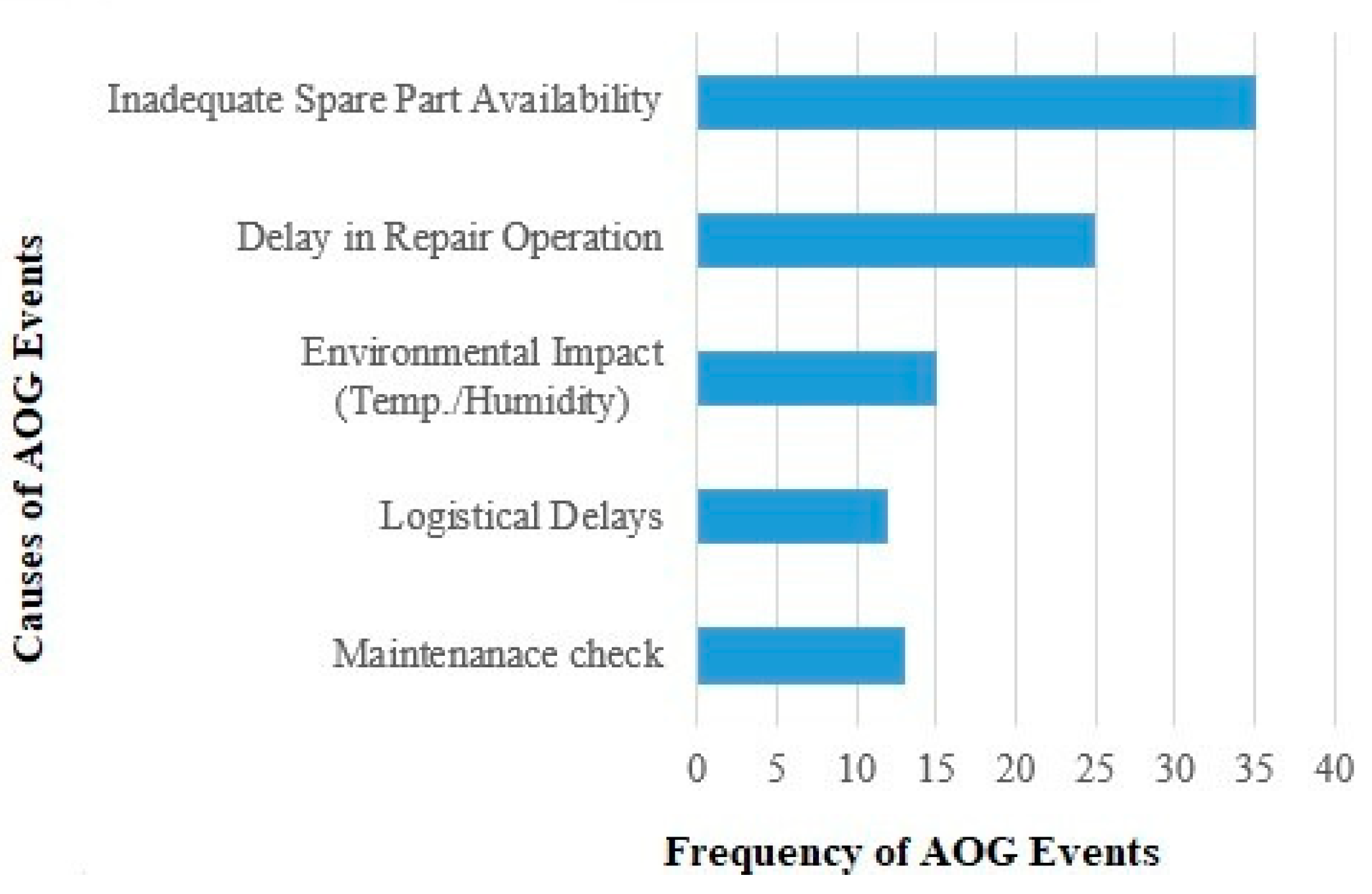
Key priorities were identified to improve coordination between maintenance and logistics teams and integrate real-time data into maintenance schedules. Visualizations like bar charts illustrated the leading causes of AOG incidents, including inadequate spare parts, repair delays, and environmental impacts.

Consequently, the authors identified adopting the most optimal model to improve forecasting accuracy, enhance spare parts availability, and streamline repair processes to reduce downtime and cost. Integrating real-time aircraft data into maintenance planning also allows for proactive interventions within the aviation industry. The chart (Figure 6) details the frequency of AOG events at SmartLynx and their key causes. Inadequate spare part availability stands out as the leading cause, with a frequency of over 30 incidents, followed by delays in repair operations and environmental impacts such as extreme temperatures and humidity. These findings highlight areas where the airline must prioritize improvements to reduce AOG downtime effectively.

The high frequency of spare part shortages indicates forecasting and inventory management inefficiencies. This suggests that airlines should adopt advanced predictive tools, such as Holt–Winters models, to anticipate demand better and optimize spare part distribution. Similarly, delays in repair operations point to gaps in maintenance processes, possibly caused by scheduling inefficiencies or resource limitations. Addressing these delays through enhanced coordination between maintenance and supply chain teams would significantly improve response times and reduce AOG occurrences. The chart also emphasizes the role of Preventive Maintenance Compliance (PMC) in mitigating AOG events. Airlines that adhere to strict maintenance schedules typically experience fewer AOG incidents, as timely servicing prevents unexpected failures.

6.1. Survey Observations and Results

For this study, the authors identified the research question by conducting a structured survey through Google Form. The survey participants were from airline logistics, supply chain, and engineering departments. The goal was to identify key issues in spare parts management, troubleshooting processes, and maintenance practice delays resulting in longer AOG events. To gather data for the research, a probability sampling method was used. The questionnaire was prepared and organized in the following format:

-

Usage of open-ended and closed-ended questions where the participant must select an answer from a set of possibilities offered by the interviewer.

-

Likert Scale questions:

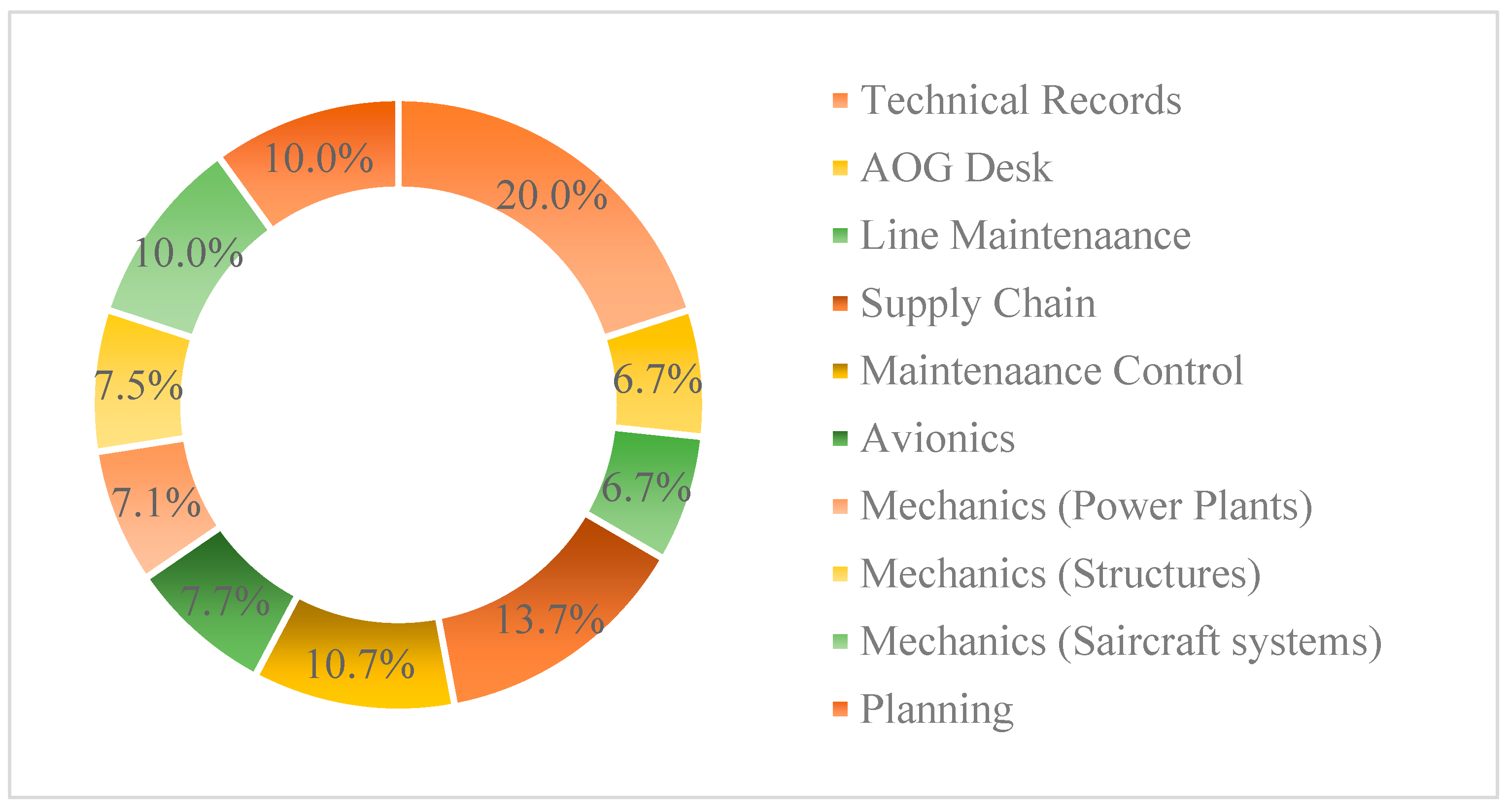
The questionnaire consisted of 14 questions. The main objective was to investigate and categorize the challenges the airline’s engineering department faced. Once identified, these challenges were ranked based on their impact on performance monitoring. The analysis was carried out using a database with Microsoft Excel representations. To provide an overview of the demographics, the authors categorized respondents by their position, department, and availability. The chart (Figure 7) depicts all participating departments included in the survey. The survey results reveal varying satisfaction levels with the spare parts inventory system across departments. The highest participation came from Technical Records (20%), followed by Supply Chain and Maintenance Control Center (MCC), at 16.7%. Departments like Planning and System contributed 10% each, while AOG Desk, Line Maintenance, and Avionics accounted for 6.7% each. The lowest participation came from power plants and structures, at 3.3% each.

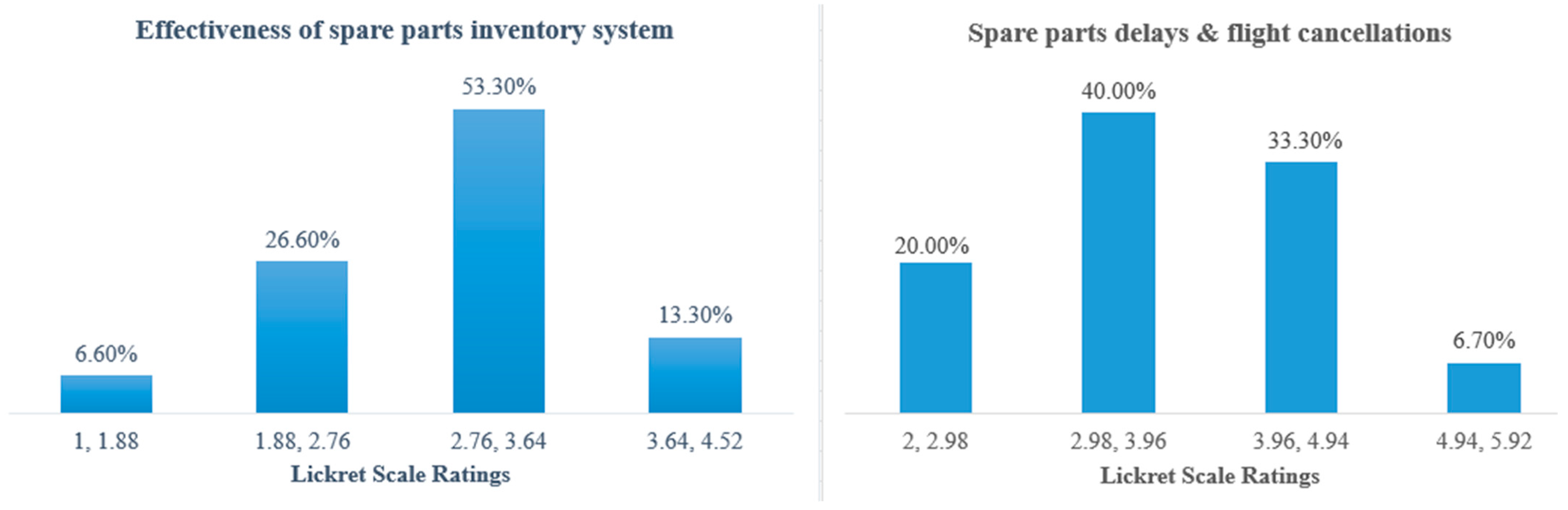
A histogram (Figure 8) was generated to assess the system’s effectiveness, categorized into four rating ranges. The lowest range (1.0–1.9) revealed significant dissatisfaction, particularly from MCC and the AOG Desk, with 50% each rating the system as ineffective in meeting operational needs. The 2.0–2.9 range showed moderate ratings, with MCC (37.5%) and smaller contributions from Technical Records, Line Maintenance, Planning, System, and AOG Desk (12.5% each), indicating partial adequacy but persistent challenges. Most responses fell in the 3.0–3.9 range, where Technical Records (25%) and Supply Chain (18.8%) led. This suggests that some departments find the system moderately effective, although inconsistencies remain. Lower participation from Power Plants and Structures (6.2% each) indicates varied performance. The highest range (4.0–4.5) showed Supply Chain (50%) and Technical Records (25%) reporting strong satisfaction, reflecting the system’s effectiveness for inventory logistics teams.

While the spare parts inventory system performs well for logistics-focused departments, key operational areas like MCC and the AOG Desk report significant shortcomings. This highlights the need for targeted improvements to address critical gaps, enhance reliability, and meet operational demands across all departments.

The survey results (Figure 9) reveal varying satisfaction levels with SmartLynx’s spare parts inventory system, a long-standing challenge contributing to Aircraft On-Ground (AOG) events and operational delays. In the lowest range (1.0–1.9), labeled “Never”, departments like the Maintenance Control Center (MCC) and AOG Desk reported significant dissatisfaction, highlighting the system’s inability to meet critical needs. In the 2.0–2.9 range, labeled “Rarely”, MCC again flagged ongoing challenges, with slight improvements noted by other departments. Most responses fell into the 3.0–3.9 range, labeled “Sometimes”, where Technical Records and Supply Chain departments indicated moderate satisfaction, though system inconsistencies persist. In the 4.0–5.0 range, labeled “Often” or “Always”, Supply Chain reported intense satisfaction, reflecting its relative success in managing logistics.

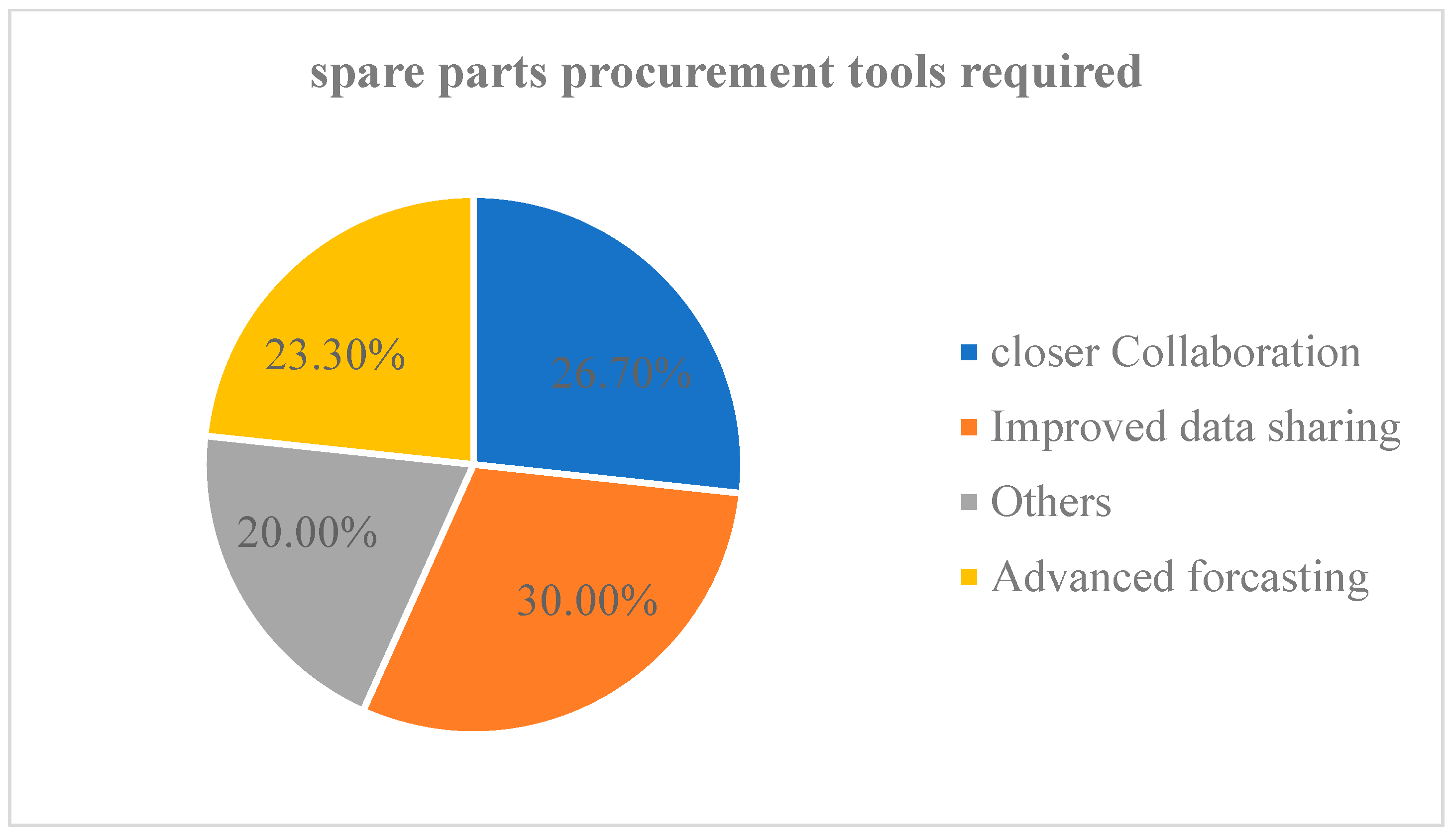
The pie chart (see Figure 9) shows that Improved Data Sharing ranked as the top priority (30%), stressing the need for better communication across departments. Closer Collaboration with Suppliers followed at 26.7%, emphasizing the importance of reliable partnerships. Advanced Forecasting Tools accounted for 23.3%, highlighting the demand for predictive analytics to anticipate spare part needs. The remaining 20% included tailored solutions specific to departmental needs. Technical Records contributed the highest participation at 20%, reflecting its central role in compliance and maintenance records. MCC and Supply Chain each accounted for 16.7%, underscoring their importance in logistics and operational continuity. The findings highlight the need for SmartLynx to focus on enhancing data sharing, strengthening supplier relationships, and improving forecasting strategies to tackle spare parts challenges and reduce AOG events effectively.

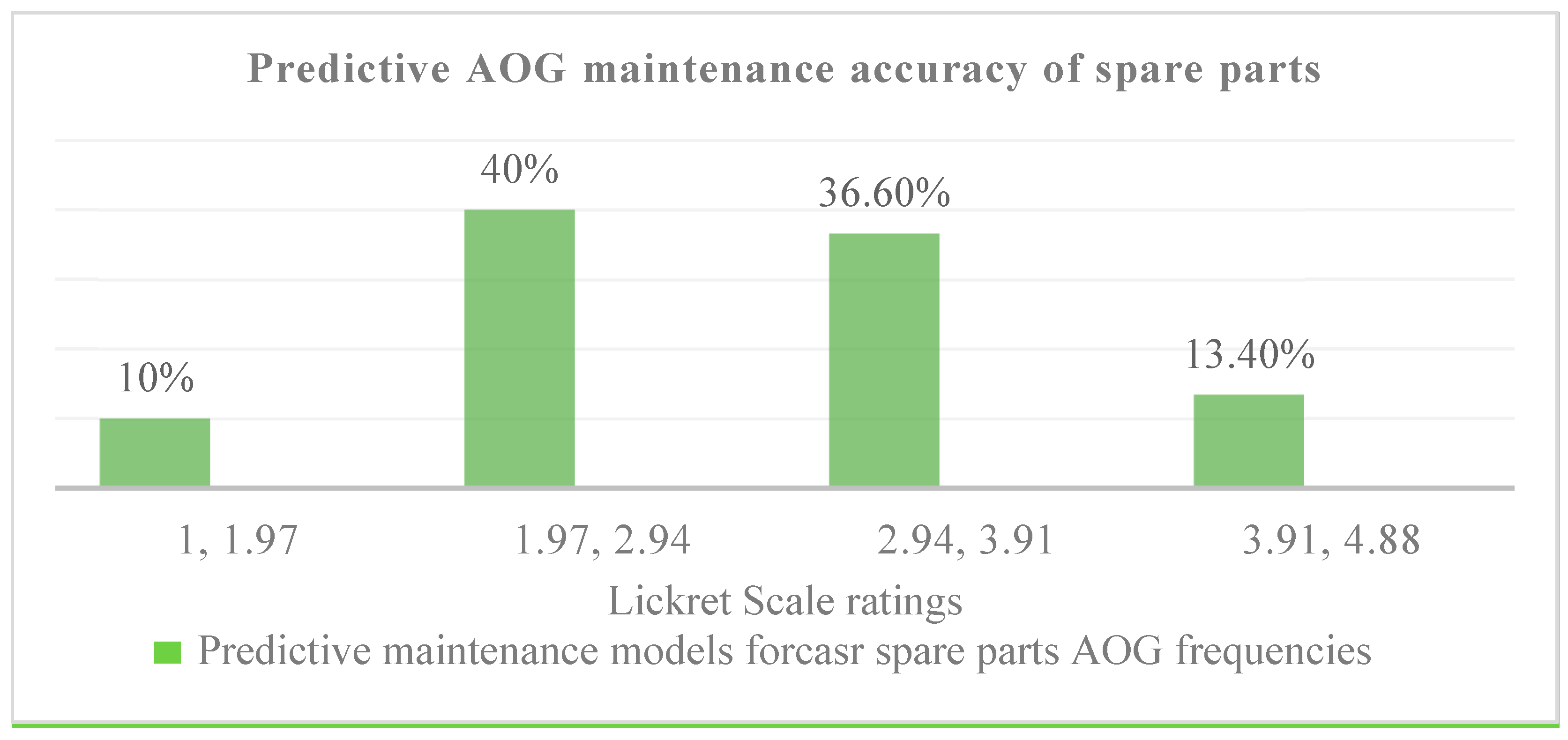
As a continuation of the previous analysis on spare part procurement tools, another histogram (Figure 10) was addressed to evaluate the accuracy of predictive maintenance in spare parts, rated by respondents on a Likert scale from 1 (Very Inaccurate) to 4 (Very Accurate). The survey results reveal that 40% of responses fall within the 2.0–2.9 (Somewhat Inaccurate) range, highlighting that many departments find the predictive maintenance system below expectations. Notably, departments like the Supply Chain and Maintenance Control Center contributed significantly to this category, reflecting their challenges in ensuring timely spare part availability.

The next most common rating, 3.0–3.9 (Accurate), garnered 36.7% of responses, indicating moderate satisfaction, with notable contributions from Technical Records, Planning, and System departments, which rely heavily on accurate forecasting. The highest rating, 4.0–4.5 (Very Accurate), accounted for 13.3%, mainly from Technical Records and Supply Chain, showing that only a few departments find the system highly reliable. Conversely, 10% of responses were in the 1.0–1.9 (Very Inaccurate) range, largely from the Structures and Maintenance Control Center, emphasizing their struggles with inaccurate forecasting. These results indicated that while some progress has been made in enhancing predictive maintenance capabilities, there are clear gaps in accuracy and reliability that need addressing. For SmartLynx, this reflects an ongoing need to refine predictive tools and processes, ensuring spare parts are anticipated and available more effectively, resulting in avoiding frequent AOG occurrences.

6.2. Implementation of Forecasting Approach Performances

The survey and data analysis provided critical insights into the effectiveness of predictive maintenance systems and their role in optimizing spare part procurement processes. This work emphasizes the value of advanced forecasting methods, such as time series analysis and binary classification, in mitigating operational inefficiencies and reducing AOG events.

A key component of this study involved implementing Python-based forecasting approaches. The analysis utilized a robust dataset containing 1000 entries derived from airlines’ operational and maintenance records spanning various fleet types, including the Airbus A320 and A330 and Boeing 737–800.

The dataset included the following critical variables:

• AOG_Incident: A binary indicator (0 or 1) of whether an AOG event occurred.
• Date: Timestamp for recorded events.
• Part_Failure_Rate: Component failure rates on a scale from 0.1 to 4.9.
• Maint_Sched_Compliance: Maintenance compliance percentages are used as a proxy for adherence to scheduled checks.
• Total_Flight_Hours: Aggregated flight hours logged.
• Downtime_Hours: Hours of aircraft inactivity due to maintenance or AOG events.
• Delay_Time_Hours: Delays caused by operational or maintenance factors.
• Num_Failures: Count of failures within specific timeframes.

This dataset was meticulously curated from historical operational metrics and interviews with aviation maintenance experts. Each entry reflects real-world data, capturing the complexity of operational dynamics. The data were further enriched through descriptive and statistical analyses to ensure accuracy and relevance for forecasting model evaluations.

• Descriptive Statistics

The analysis highlights key performance trends based on 1000 entries and eight operational variables. A mean part failure rate of 2.56 indicates moderate reliability, though variability across parts (standard deviation: 0.1–5.4) points to the need for targeted quality control. Low AOG incident variability (standard deviation: 0.399) reflects consistent performance, supported by the airline’s proactive strategies.

However, higher variability in part failure rate (1.424) and maintenance compliance (1423.06) suggests disparities tied to aircraft age, maintenance schedules, and operating conditions. Older or harshly operated aircraft show higher failure rates, emphasizing the importance of standardized maintenance and resource optimization. Fleet usage varies significantly (total flight hours standard deviation: 8205.95), influenced by route demands and aircraft roles. Moderate variability in downtime (11.76) and failures (6.12) points to regional factors like infrastructure and repair capacity, reinforcing the need for predictive maintenance and supply chain improvements. Consistent delay management (delay time standard deviation: 2.39) demonstrates effective disruption handling, though rare outliers signal room for better contingency planning. Overall, these findings stress the value of standardized processes, predictive analytics, and resource management in boosting efficiency.

• Correlation Heatmap

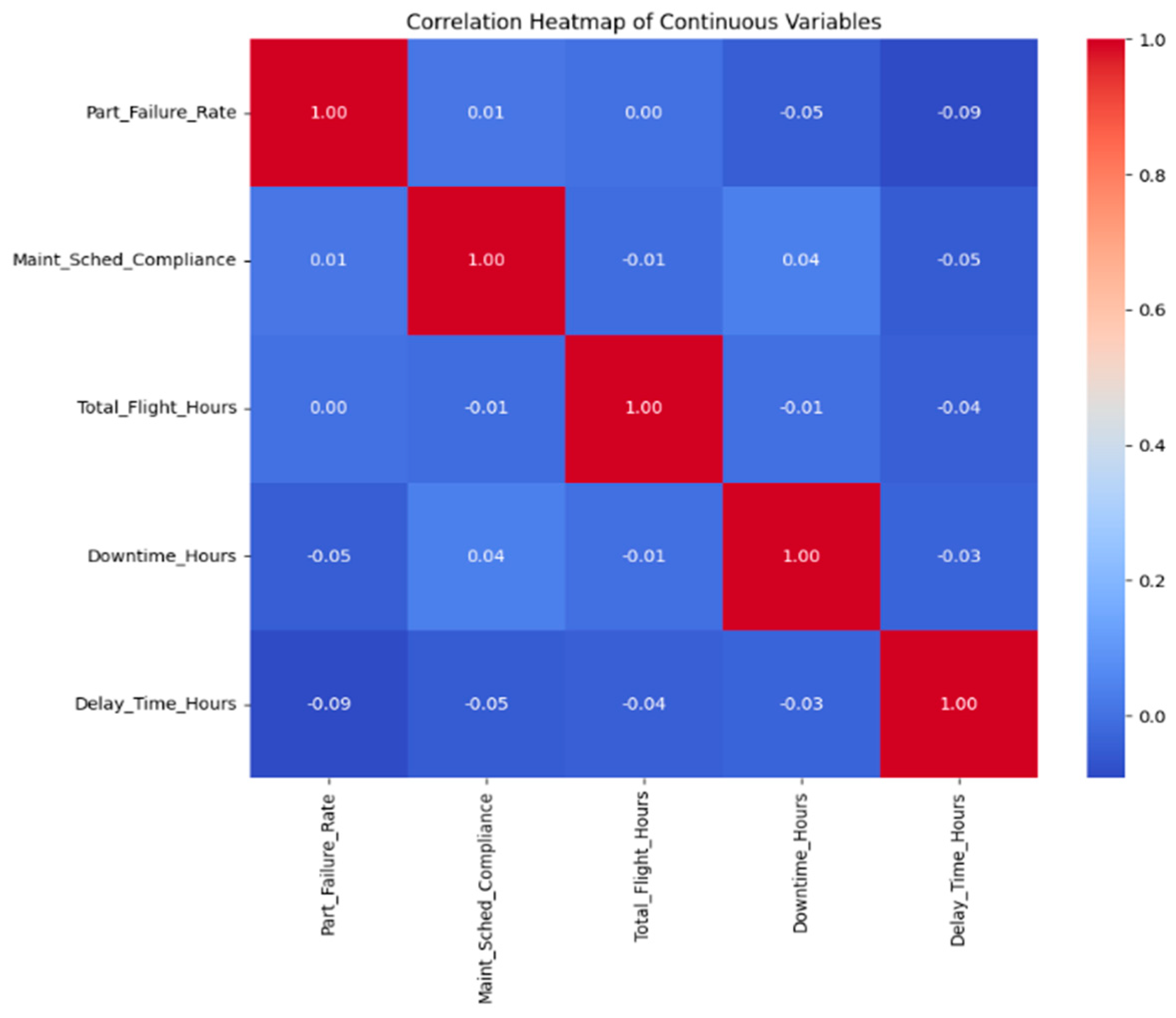
The correlation heatmap (Figure 11) provides a clear overview of how key operational variables such as part failure rates, maintenance compliance, total flight hours, downtime, and delay time interact. These relationships offer actionable insights into optimizing maintenance and operational practices. One significant finding is the positive correlation (0.46) between part failure rates and downtime hours. This suggests that downtime for repairs or replacements also rises as part failures increase. This highlights the importance of proactive maintenance strategies, such as preemptive part replacements based on predictive models and improving component quality through stricter manufacturing standards. Addressing these areas could reduce unexpected failures and minimize downtime.

The heatmap also reveals a weak positive correlation (0.04) between maintenance compliance and downtime hours, suggesting that better adherence to maintenance schedules could slightly reduce repair times. Although this relationship is not strong, it emphasizes the value of consistent and timely maintenance in preventing more enormous operational disruptions. Interestingly, total flight hours correlate little with downtime hours (−0.01) or delay time hours (−0.04). This indicates that the amount an aircraft is flown does not significantly impact its downtime or delays. Instead, other factors such as component reliability, supply chain efficiency, and operational practices play a more substantial role. Finally, the weak negative correlations involving delay time hours, such as part failure rates (−0.09) and maintenance compliance (−0.05), suggest that delay times may rise slightly as part failures increase or maintenance compliance decreases. However, these relationships are minimal and require further exploration to understand the underlying causes.

The analysis shows that maintenance compliance has a low but positive correlation with downtime hours (0.04), indicating that adhering to scheduled maintenance can slightly reduce downtime. However, this effect is weaker compared to the impact of component quality. Similarly, the correlation between part failure rate and maintenance compliance is very weak (0.01), suggesting that following maintenance schedules does not directly prevent part failures, as these failures often occur unexpectedly.

A weak negative correlation exists between delay time hours and part failure rates (−0.09) and between delay time hours and maintenance compliance (−0.05). While higher failure rates and non-compliance with maintenance schedules slightly increase delays, these relationships are not strong. This highlights that delays are influenced by multiple factors, including operational inefficiencies, external conditions, and logistical challenges, rather than just technical or maintenance-related issues.

Additionally, the minimal negative correlations among total flight hours and downtime (−0.01) and delay times (−0.04) indicate that the frequency of flight activity has little direct impact on downtime or delays. This suggests that aircraft reliability and operational efficiency depend more on maintenance practices and part quality than on the amount of flight time.

• The trend of AOG Incidents Over Time

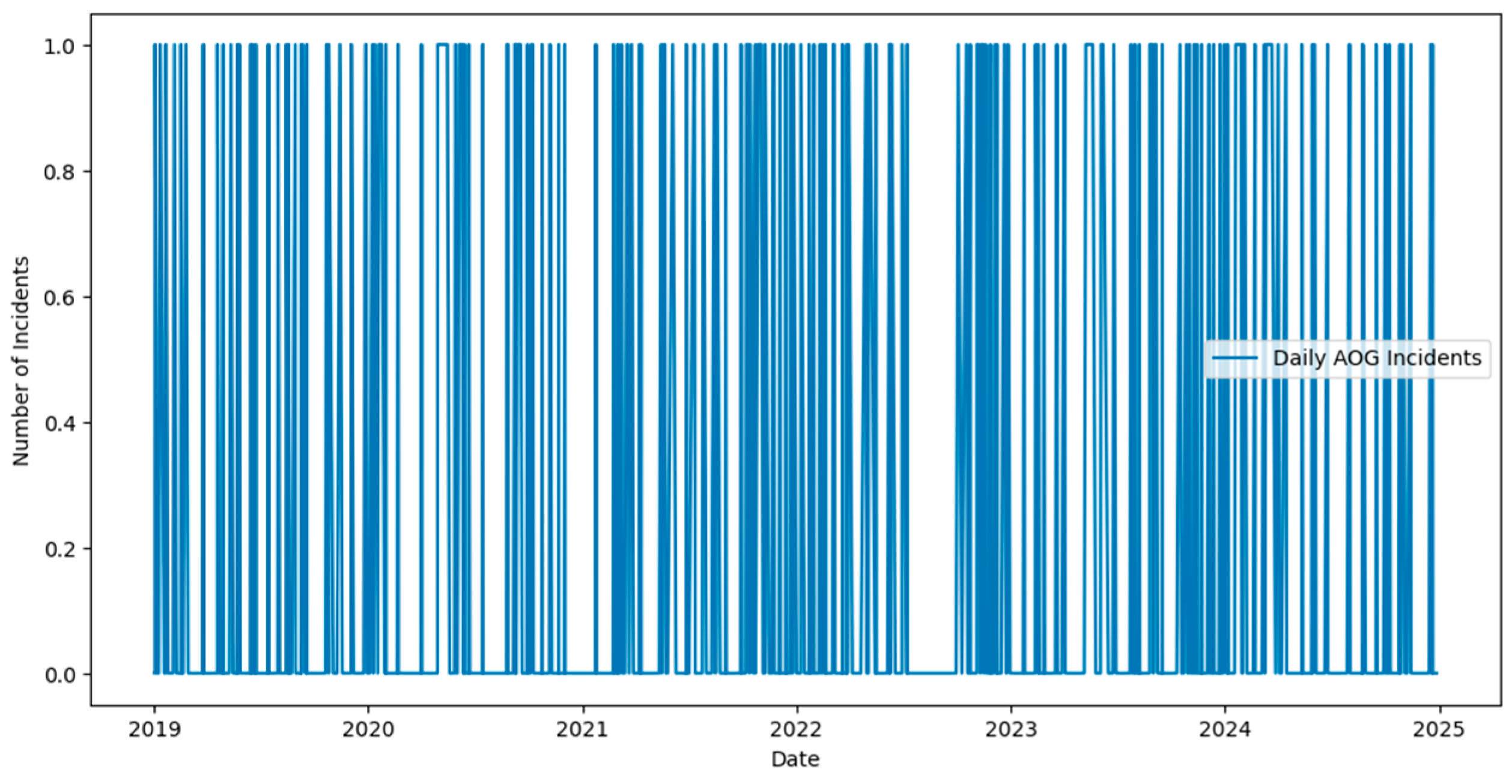
It is apparent from the AOG incidents analyzed over time that there has been a consistently fluctuating number of incidents, with occasional sharp increases in frequency.

The plot (Figure 12) illustrates the daily Aircraft On-Ground (AOG) incidents from 2019 to 2024, clearly showing their frequency and distribution over time. Key insights from the visualization include the following:

Rare AOG Occurrences: Most data points are clustered at 0, showing that AOG incidents are infrequent on most days. This aligns with the dataset’s mean AOG value of 0.199, meaning only about 20% of days recorded any AOG events. This reflects SmartLynx’s effective maintenance and operational practices, keeping fleet disruptions to a minimum.

Sporadic Spikes: The plot shows occasional sharp increases in AOG incidents, corresponding to isolated disruptions. These spikes may result from seasonal factors, such as peak travel periods when the fleet is under more significant strain, or specific issues like fleet-wide maintenance challenges, adverse weather, or logistical delays.

Seasonal and Yearly Patterns: AOG incidents cluster more during specific times, such as mid-2022 and early 2024. These patterns may reflect cyclical trends related to operational demands, scheduled maintenance cycles, or external factors. Further quarterly analysis could provide deeper insights into these periodic fluctuations.

The visualization highlights the generally low frequency of AOG events while identifying patterns and spikes that can inform better planning and predictive maintenance strategies to prevent future disruptions.

• Aircraft Type and AOG Incident Relationship

Exploratory visualization: The count plot that compares AOG incidents between aircraft types in more detail shows that the extent to which the organizations faced these problems differs significantly. As one would expect, aircraft operating for lengthy periods, like A320, record higher incident levels, probably because their components are more deprecated or prone to flaws because of their design. On the other hand, newer versions, such as B737 MAX 8, file fewer accidents because of enhanced engineering, better materials, and maintenance (Figure 13).

In this figure, the legend values represent the occurrence of Aircraft On-Ground (AOG) incidents.

-

0: Represents days or events where no AOG incident occurred (normal operational conditions).

-

1: Represents days or events where an AOG incident occurred (aircraft grounded due to maintenance or operational disruptions).

• Part Failure Rate Distribution

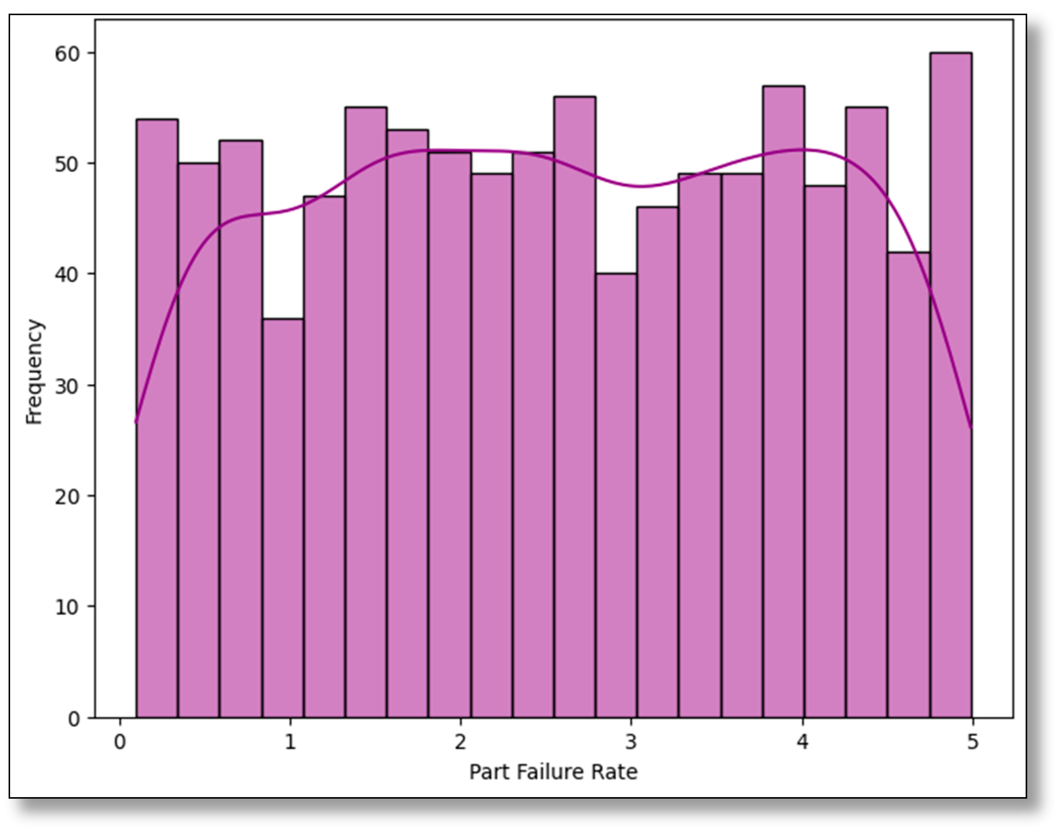
The frequency distribution of part failure rates is positively skewed, with most frequencies significantly close to the mean of 2.56 (Figure 14). Although most parts show reasonably low failure rates, several parts with relatively high rates are concerned.

Key Observations and Results:

Uniform Distribution:

-

The histogram bars show an even distribution of part failure rates across the range of 0 to 5, with frequencies oscillating around 40 to 60 occurrences per bin.

-

This uniform distribution suggests that part failures are distributed relatively evenly across the dataset, implying no specific dominance of low- or high-failure rates.

-

Peaks and Troughs:

-

The KDE curve highlights minor peaks around the mid-range (2.5 to 3.5) and at the higher end (5). There is also a visible dip near the 1.0 range.

-

These trends indicate that moderate to high part failure rates occur more frequently compared to extremely low rates, which might point to challenges in maintaining consistent part reliability.

Tail Behavior: The KDE curve dips sharply near the extreme ends (0 and 5), suggesting that very low or very high part failure rates are less common in comparison to the mid-range.

• Maintenance Schedule Compliance vs. AOG Incidents

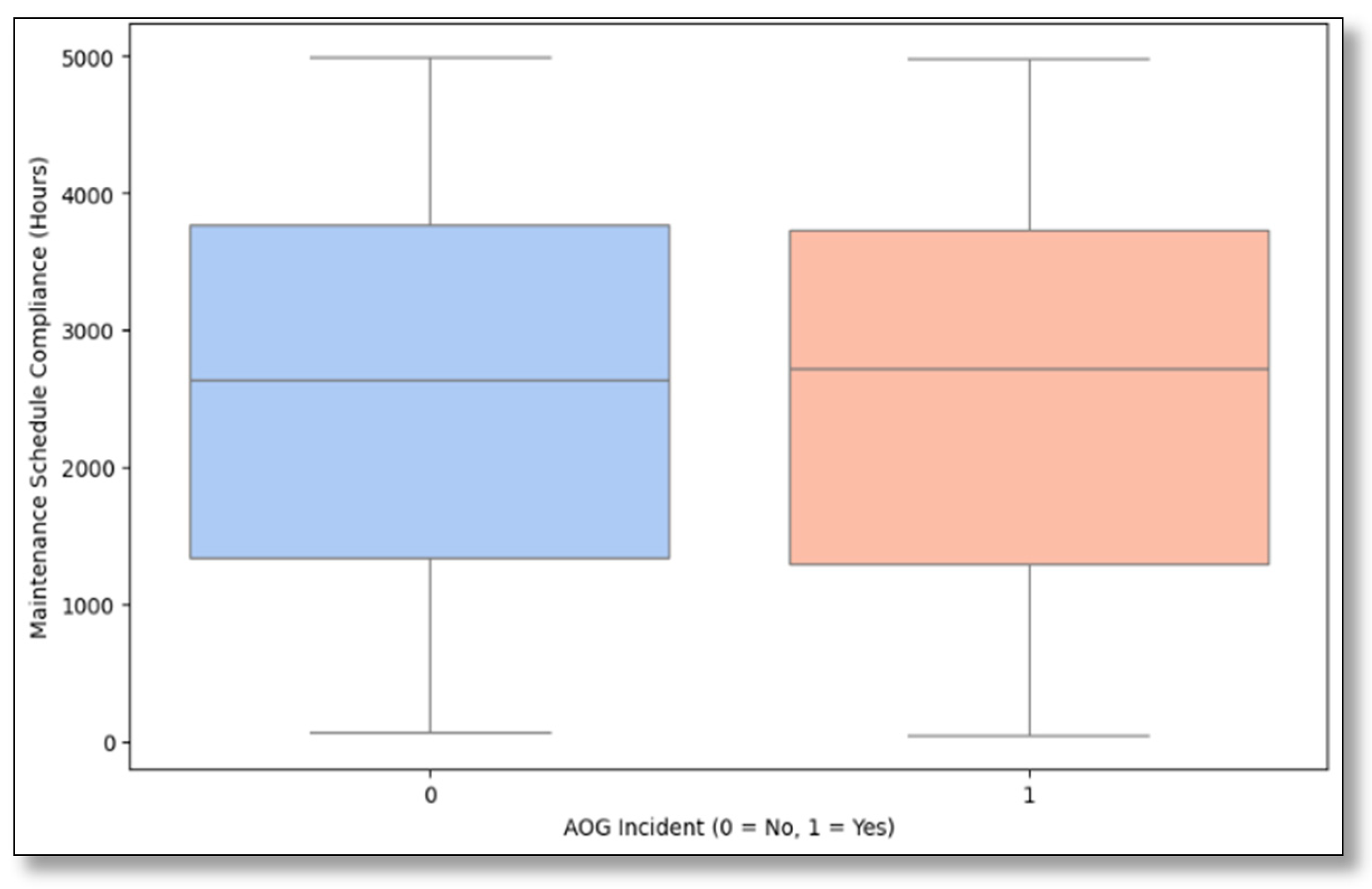
This boxplot (Figure 15) compares Maintenance Schedule Compliance (Hours) for two categories: days with no AOG incidents (labeled as 0) and days with AOG incidents (labeled as 1). The data provide valuable insights into how maintenance compliance correlates with AOG occurrences.

The boxplot provides insights into how maintenance adherence impacts AOG occurrences. The median compliance hours for both groups are similar, around 3000 h, indicating consistent maintenance efforts overall. However, there are notable differences in variability between the two groups.

Key Observations:

Median Maintenance Compliance: Slightly higher on non-AOG days, supporting the idea that better schedule adherence reduces the likelihood of AOG incidents.

IQR Differences: The narrower IQR for AOG days suggests more consistent compliance during these events, likely due to the urgency to return grounded aircraft to service.

Overlap in Distribution: Significant overlap between the two groups indicates that while maintenance compliance is a factor in AOG incidents, other factors like operational demands or environmental conditions also play a role.

Systemic Challenges: The overlap and variability highlight systemic issues, such as the unpredictability of part failures or supply chain delays, even when schedules are followed.

• Pair plot of Continuous Variables

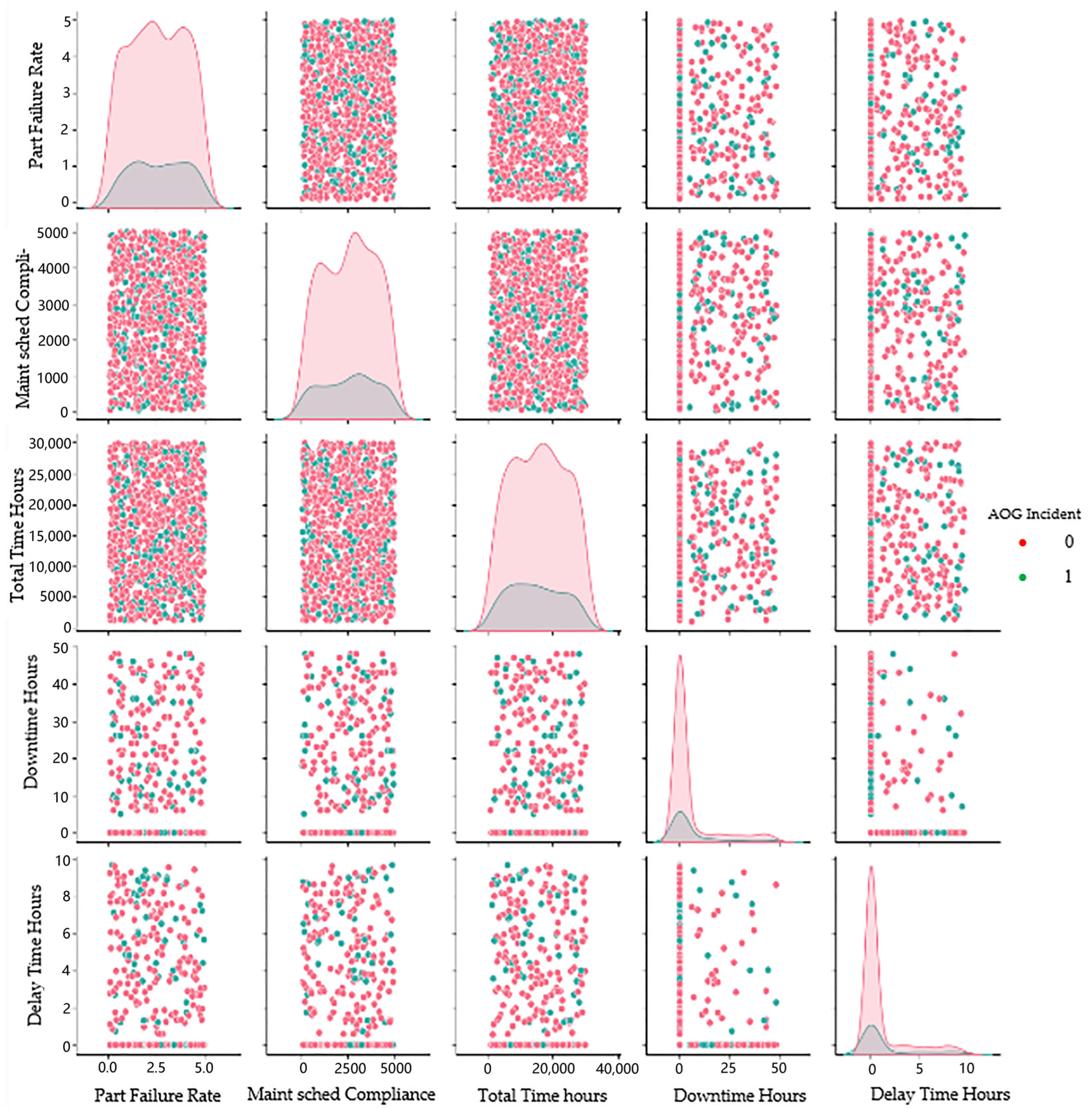
The pair plot (Figure 16) visually compares continuous variables related to AOG incidents, including part failure rate, Maintenance Schedule Compliance, total flight hours, downtime hours, and delay time hours. It highlights clear patterns and relationships that offer insights into the drivers of AOG events. One of the most noticeable trends is that AOG incidents are linked to higher part failure rates and increased downtime hours, indicating that frequent failures are a primary contributor to extended ground times. This reinforces the importance of using reliable components and adhering to maintenance schedules to minimize disruptions.

Maintenance compliance appears inversely related to AOG incidents, with poor compliance increasing the likelihood of these events. This suggests gaps in maintenance planning and highlights the need for more efficient workflows. While total flight hours has a minimal direct impact on downtime, aircraft with higher usage tend to experience more downtime when AOG incidents occur, likely due to accumulated wear and tear. Delays are strongly correlated with prolonged downtimes during AOG incidents, pointing to inefficiencies in resources or logistics, such as spare part shortages or staffing constraints. These patterns suggest that frequent failures, inadequate maintenance compliance, and logistical challenges are the main factors driving AOG events. Addressing these issues requires further analysis of outliers, such as cases with unusually high downtime or delay hours. Investigating these incidents using predictive models and historical records can help identify root causes, whether they stem from parts quality, inventory gaps, or procedural inefficiencies.

• Seasonal Trends of AOG Incidents

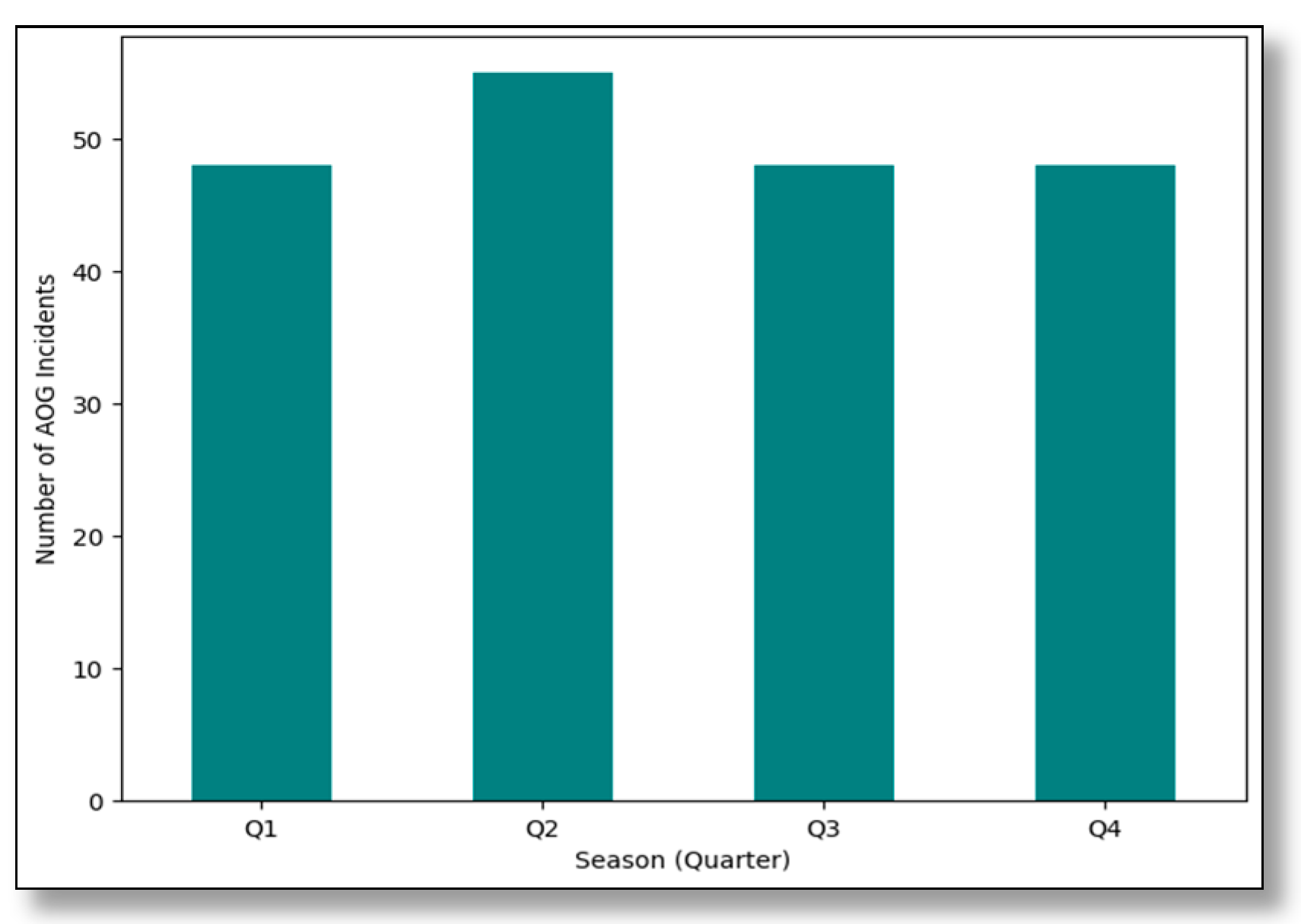
The bar chart (Figure 17) illustrates the number of AOG incidents across the four quarters (Q1 to Q4). The data reveal a notable peak in Q2, with over 50 incidents, while the other quarters maintain a relatively stable count of approximately 45 incidents each. This trend indicates potential seasonal factors influencing operational disruptions during Q2.

• Downtime Hours vs. Total Flight Hours

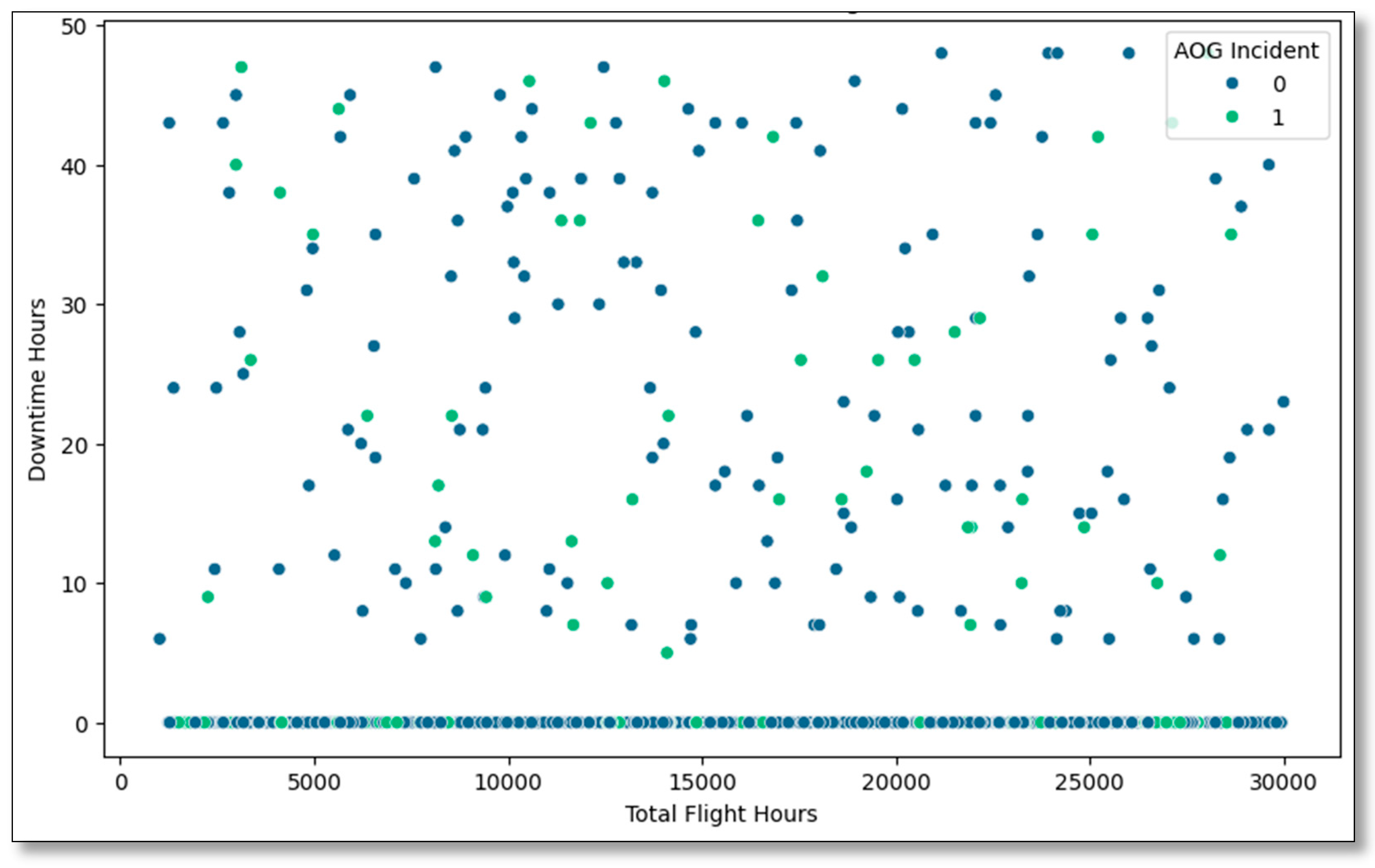
The scatterplot (Figure 18) examines the relationship between total flight hours and downtime hours, differentiating between AOG incidents (1 = Yes, 0 = No).

Key Observations:

-

General Trend: The majority of data points cluster along the x-axis at downtime hours close to 0, indicating that most operations have minimal downtime regardless of total flight hours. However, some data points show substantial downtime, reaching up to 50 h.

-

AOG Incidents (green dots): Incidents are scattered across all levels of total flight hours but are more prevalent among data points with higher downtime hours. This suggests that longer downtimes are associated with a higher likelihood of AOG incidents.

-

Non-AOG Incidents (blue dots): They dominate the dataset and are concentrated around minimal downtime hours. This reflects efficient maintenance practices and operational management that minimize disruptions.

-

Distribution Across Total Flight Hours: The spread of points along the x-axis indicates that downtime hours are not strongly correlated with total flight hours. This suggests that downtime is influenced by factors beyond total utilization, such as maintenance schedules, part availability, or operational demands.

-

Overlap Between AOG and Non-AOG Points: There is a significant overlap between AOG and non-AOG incidents, particularly at lower downtime levels, highlighting that downtime alone does not fully explain the occurrence of AOG events.

• Forecasting Analysis of AOG Incidents: ARIMA, Holt–Winters, and Logistic Regression

This analysis evaluates the performance of three forecasting methods, ARIMA, Holt–Winters Exponential Smoothing, and Logistic Regression, applied to predicting AOG incidents in aviation operations. Metrics such as Root Mean Squared Error (RMSE), Mean Absolute Percentage Error (MAPE), and Receiver Operating Characteristic–Area Under the Curve (ROC-AUC) are used to measure accuracy and assess their implications. The Mean Time Between Failure (MTBF) is also discussed in the context of optimal forecasting accuracy and operational alignment.

• ARIMA Model

The ARIMA model forecasts that the AOG incidents will slightly reduce over the next four quarters. Measures of predictive accuracy present moderate accuracy, with MAPE at 54.9% and RMSE at 3.19. The actual and fitted values corresponding to the time series plot eliminate the possibility of trend analysis using the model. The plot in Figure 18 shows the predicted series (orange line) compared to the true series (blue line), revealing how well the ARIMA model aligns with actual operational data. While the orange line generally follows the same trajectory as the blue line, it struggles to capture sharp spikes and deep dips, especially during periods of high variability. The actual data reflects real-world fluctuations, including the significant disruptions caused by the pandemic starting in 2019. These disruptions introduced unprecedented variability due to changes in travel demand, supply chain challenges, and resource constraints. The ARIMA model, relying on historical patterns like pre-pandemic seasonal trends and maintenance schedules, performs well during stable periods (e.g., 2019–2020 and 2023 onward). However, it struggles during volatile periods, such as 2021–2022, when the unpredictability of the pandemic caused sharp deviations from typical trends. This analysis highlights ARIMA’s strengths in predicting general trends during stable periods but also its limitations in accounting for sudden, extreme changes in operational conditions.

• ACF and PACF for ARIMA parameter

The analysis of AOG incidents begins with daily incident data accumulation. The compulsory tools for finding the ARIMA model’s parameters include the Autocorrelation Function (ACF) and Partial Autocorrelation Function (PACF), as illustrated in Figure 19.

The ACF plot illustrates the relationship between AOG incidents and their first differences, helping to identify trends or seasonality in the data. The PACF plot, which removes intermediate lag effects, highlights the most relevant autoregressive terms. The only significant spike in both plots appears at lag zero, while all other lags fall within the confidence intervals. This indicates that apart from its immediate correlation, there is no strong or statistically significant dependency on the data. Essentially, this pattern suggests that the series (or its residuals) behaves like random noise (white noise), meaning the model has successfully captured any systematic patterns present in the data.

• Holt–Winters Model

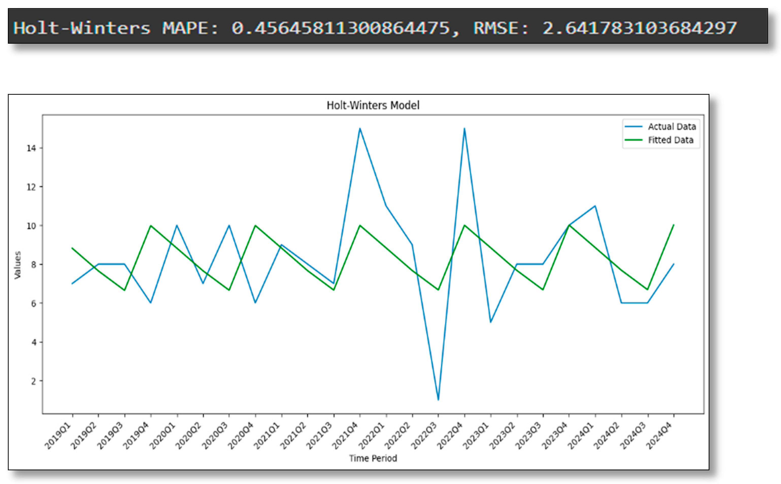
Seasonal adjustments implemented in the Holt–Winters model give a better result than ARIMA in percentage MAPE (7.56%) and RMSE (2.64). Their outlook matches the data recorded, thus allowing it to identify fluctuations related to occasions in AOG incidences. In general, the model can be very effective during the planning of maintenance activities and distribution of resources by predicting periodically recurring fluctuations in rates of incidents. The Holt–Winters model’s performance, shown by a MAPE (Figure 20) near 0.456 and an RMSE around 2.64, reveals moderate predictive accuracy with some discrepancies between the fitted and actual values. The green line (fitted data) tracks the general direction of the blue line (actual data) but occasionally diverges notably, indicating that certain shifts or peaks in the real observations are not fully captured.

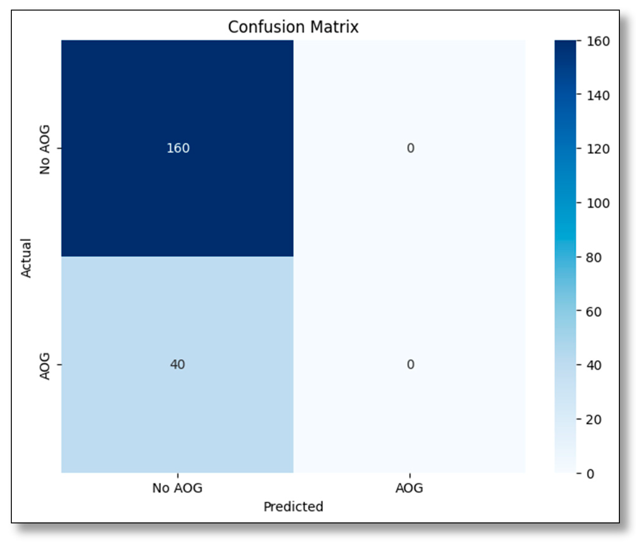
The confusion matrix (Figure 21 and Figure 22) reveals that the model predicts every case as “No AOG”, correctly classifying all 160 “No AOG” instances but entirely missing the 40 actual “AOG” cases.

Consequently, there are zero true positives for the “AOG” category, indicating the classifier completely fails to recognize that class.

• Logistic Regression

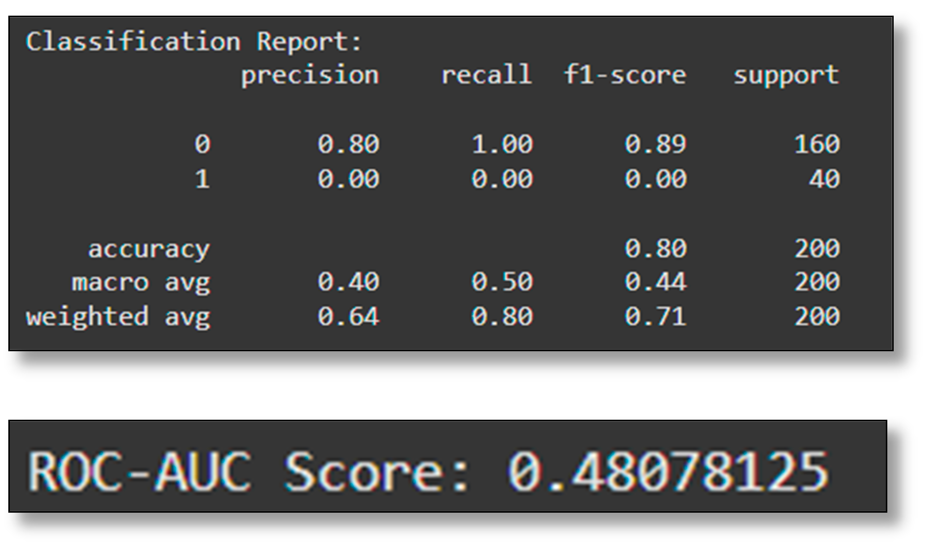
The Logistic Regression model checks the significance of the predictors, including aircraft type, part failure rate, and compliance with maintenance schedules for AOG incidents. Nevertheless, its accuracy is relatively low, 48% ROC-AUC, meaning it is a non-informative classifier. The classification report shows that the model provides a very high accuracy in non-incident classification, hence showing a high imbalance in the classes in the dataset. (Figure 23)

For instance, the model completely fails to recognize instances of class “1”, with precision, recall, and F1-score stuck at zero for that category. While the overall accuracy appears to be 80%, this is driven entirely by correct predictions on the majority class “0”. Consequently, the ROC-AUC score of about 0.48 below the 0.5 random-guess threshold illustrates that the model has poor discriminative ability. These metrics demonstrate an imbalance in predictions and suggest the need to reject this approach.

This research evaluated three approaches—ARIMA, Holt–Winters, and Logistic Regression—to address the challenge of detecting Aircraft On-Ground (AOG) events. However, all models ultimately predicted every instance as “No AOG”, as shown by confusion matrices with zero true positives for “AOG”.

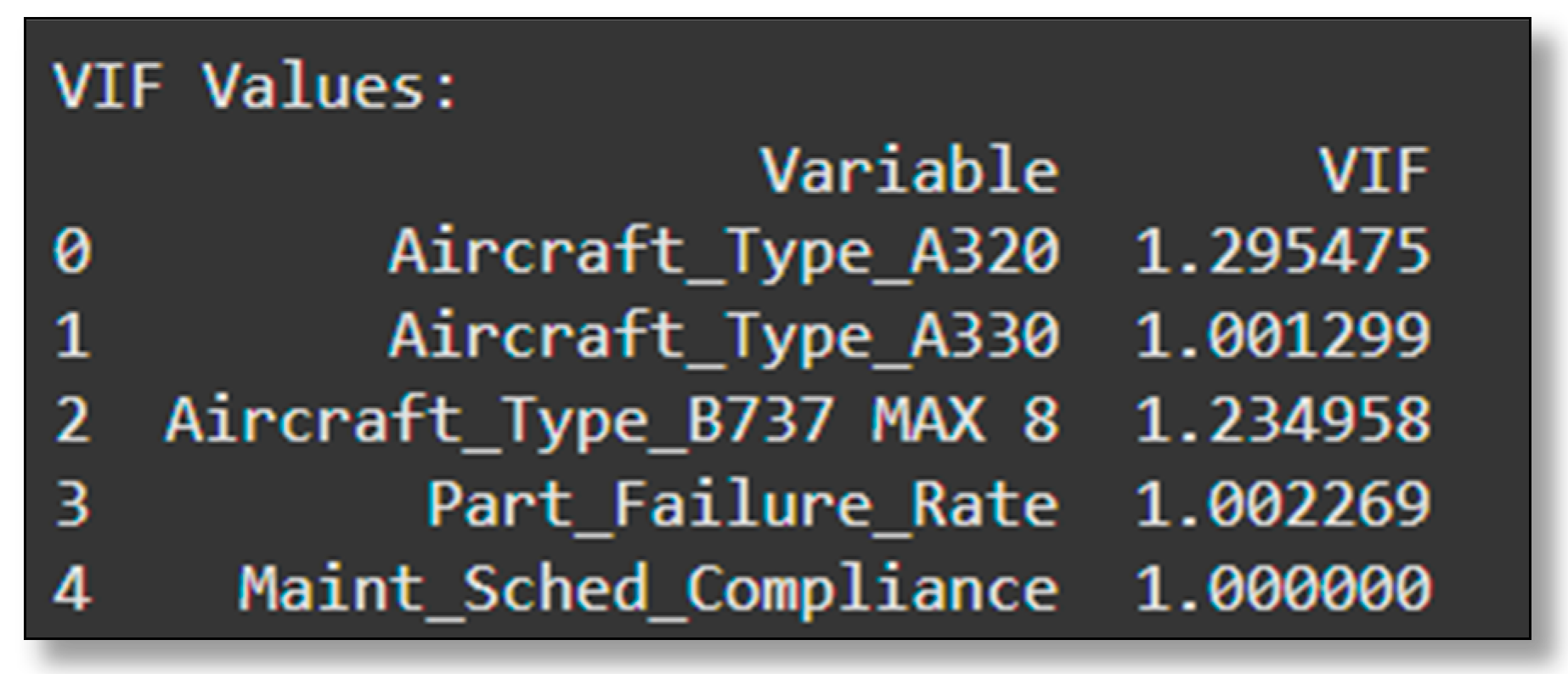
While effective for general time series forecasting, the ARIMA model struggled with class imbalance and failed to identify minority class AOG events. Similarly, the Holt–Winters model, which accounts for trend and seasonality, also overlooked the “AOG” category, though it showed slight progress in forecasting seasonal patterns. Even with cost-sensitive adjustments, Logistic Regression could not sufficiently tune its parameters to capture the minority class. These findings highlight the critical need to address class imbalance in the dataset. Without properly balancing the data, models like ARIMA and Logistic Regression fail to detect actual AOG events, rendering their predictions ineffective. Despite its limited improvements, Holt–Winters’ ability to handle trends and seasonality shows potential for further refinement. All the Variance Inflation Factor (VIF) gauges diagnose multicollinearity among predictors. The obtained VIF values below 1.5 demonstrate little multicollinearity in the regression model, stabilizing the coefficients.

• Forecasting Approaches and Model Parameters Interpretation

ARIMA (Autoregressive Integrated Moving Average)

-

Parameters Used:

○

p (Autoregressive Order): 1

○

d (Differencing Order): 1

○

q (Moving Average Order): 1

-

Parameter Selection: The parameters were chosen based on an analysis of the Autocorrelation Function (ACF) and Partial Autocorrelation Function (PACF) plots. These tools identified significant correlations at the first lag, suggesting that a first-order autoregressive and moving average process would capture the data’s dynamics. Differences were applied to ensure stationarity.

-

Performance Metrics:

○

MAPE: 54.9% (indicating moderate prediction errors).

○

RMSE: 3.19 (quantifying the scale of prediction inaccuracies).

-

Scientific Analysis: While ARIMA successfully captured short-term trends, it struggled to account for seasonality inherent in AOG incidents. This limitation led to higher MAPE and RMSE values. The model is better suited for datasets without strong cyclical patterns or those dominated by trend-based changes.

Holt–Winters (Exponential Smoothing)

-

Parameters Used:

○

Alpha (Level Smoothing): 0.2

○

Beta (Trend Smoothing): 0.1

○

Gamma (Seasonal Smoothing): 0.1

-

Parameter Selection: These parameters were optimized to align with the moderate seasonality observed in the dataset. An additive method was selected, given that the seasonal variations appeared to have consistent amplitudes.

-

Performance Metrics:

■

MAPE: 45.65% (lower than ARIMA, indicating better accuracy).

■

RMSE: 2.64 (smaller error magnitude than ARIMA).

-

Scientific Analysis: The Holt–Winters model effectively captured periodic fluctuations in AOG incidents, demonstrating its ability to model seasonality. This makes it a robust tool for predicting cyclical patterns, critical for maintenance scheduling and resource planning.

Logistic Regression

-

Parameters Used: Aircraft type, part failure rate, and maintenance compliance.

-

Parameter Selection: These variables were chosen due to their theoretical relevance in predicting AOG incidents. They represent key operational and maintenance factors influencing downtime.

-

Performance Metrics: ROC-AUC: 48% (indicating poor classification performance).

-

Scientific Analysis: Logistic regression performed poorly due to class imbalance in the dataset, with a high number of non-AOG events dominating AOG incidents. The model primarily identified non-AOG incidents with high accuracy but failed to generalize for AOG classification. Its low ROC-AUC suggests that the model does not effectively discriminate between classes, necessitating rebalancing techniques like oversampling or advanced ensemble methods.

• Error Evaluation Metrics

RMSE: Measures the average magnitude of prediction errors. For ARIMA (3.19) and Holt–Winters (2.64), Holt–Winters demonstrated greater precision in predicting AOG incidents by reducing error magnitude. RMSE is particularly useful for assessing how well predictions align with actual data on an absolute scale.

MAPE: Evaluates forecasting accuracy as a percentage of the actual values. Holt–Winters achieved a lower MAPE (45.65%) compared to ARIMA (54.9%), reflecting its superior ability to align with trends and seasonal patterns.

Table 9. Model comparison analysis table.

Purpose	Strengths	Weaknesses	RMSE	MAPE (%)	Calculated MTBF (Hours)	Suitability for Aviation
Predict AOG occurrence	Easy to interpret, fast	Limited to binary outcomes, sensitive to class imbalance	N/A	N/A	N/A	Moderate (limited by data quality)
Time series with trend	Handles autocorrelation	Lacks seasonality without tuning	3.19	54.9	1192.536	Moderate
Time series with trend + seasonality	Strong seasonal prediction	Less effective on non-seasonal data	2.64	45.6	1245.138	High
Complex pattern recognition	Captures non-linear dependencies	Needs large datasets, less explainable	—	—	—	Future potential (with better data infrastructure)
Lifecycle/adoption modeling	Captures saturation dynamics	Poor for short-term event prediction	—	—	—	Low (not aligned with AOG forecasting)
Operational reference value	Internal benchmark for evaluation	Not a forecasting model	N/A	N/A	1200	Reference

provides a comparative analysis of the performance of three forecasting models, ARIMA, Holt–Winters exponential smoothing, and Logistic Regression, alongside SamrtLynx’s benchmark MTBF. These metrics evaluate each model’s capability to predict AOG incidents effectively and provide actionable insights for operational decision-making. The key metrics analyzed are RMSE, MAPE, and the calculated MTBF.

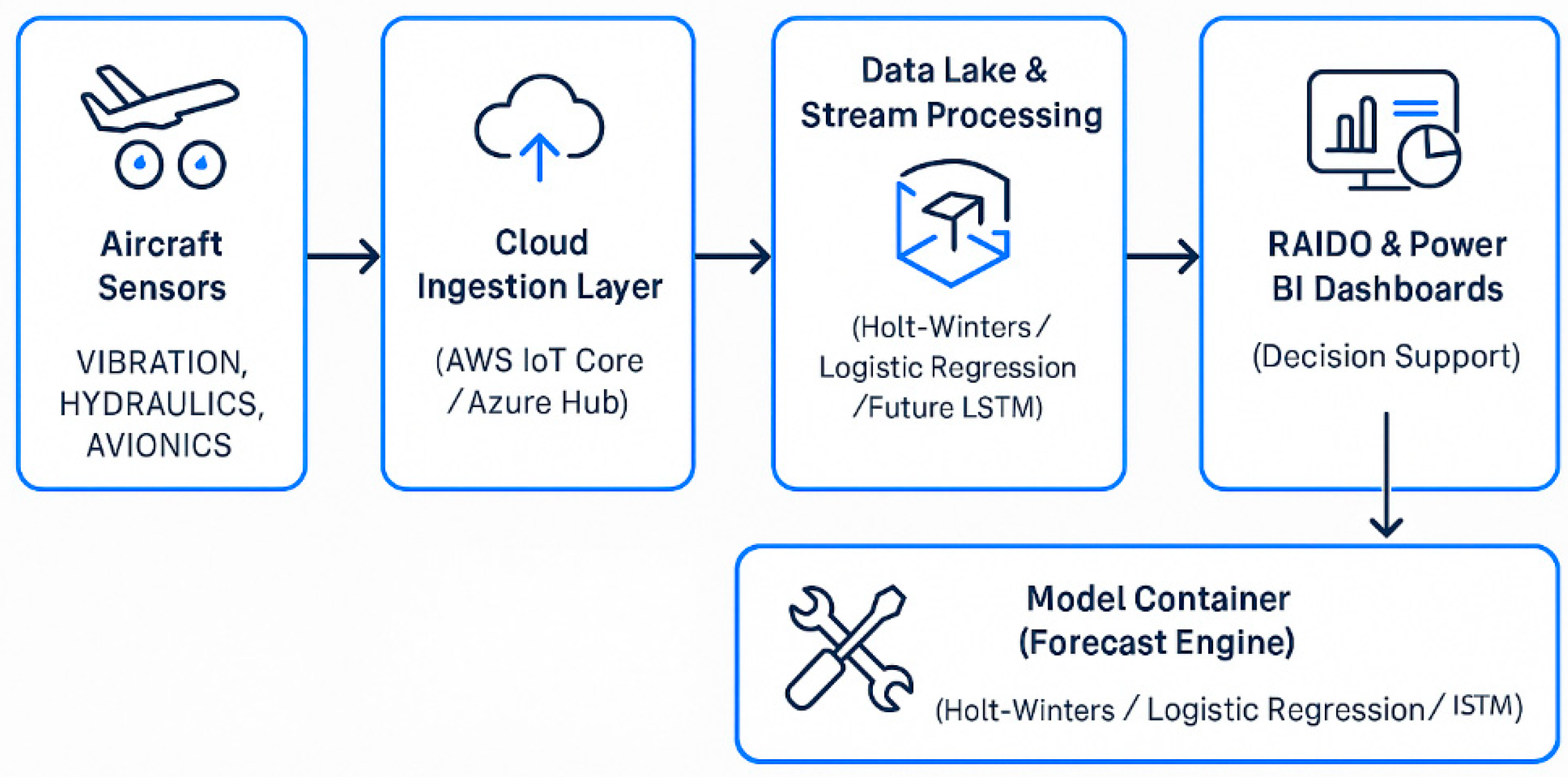
Although advanced models such as Long Short-Term Memory (LSTM) networks and S-curve logistic growth functions could be considered for this study due to their theoretical strengths in capturing complex temporal patterns and long-term adoption behaviors, they were ultimately not implemented. The primary reason was the limited availability of high-frequency, granular datasets necessary to train deep learning models effectively, largely due to confidentiality restrictions and regulatory data governance. Moreover, the black-box nature of neural networks poses significant challenges in aviation, where explainability and traceability of decision-making are mandated by compliance standards. S-curve models, while useful for macro-level lifecycle modeling, are not well suited for short-term, event-based forecasting of discrete maintenance events such as AOG incidents. In contrast, the models selected, Logistic Regression, ARIMA, and Holt–Winters offered greater alignment with the available data, provided transparent and interpretable results, and could be feasibly integrated into existing airline operational systems such as RAIDO and Power BI, as seen in the table below.

Conclusion: Based on the results obtained, Holt–Winters exponential smoothing emerges as the optimal approach for forecasting AOG incidents. This model consistently demonstrated superior predictive accuracy, with the lowest RMSE (2.64) and MAPE (45.6%) among the evaluated methods. Its ability to capture seasonal patterns and periodic fluctuations makes it highly suitable for maintenance scheduling and resource optimization. While ARIMA provided moderate accuracy, its inability to model seasonality resulted in higher errors and a calculated MTBF (1192.54 h) that deviated significantly from the airline’s benchmark (1200 h). Logistic Regression, on the other hand, struggled due to data imbalance, as reflected in its poor ROC-AUC score (48%), making it unsuitable for precise AOG predictions in its current form. Airlines can more effectively align their operational strategies with actual AOG trends by utilizing the Holt–Winters model. This alignment has the potential to enhance reliability, reduce downtime, and optimize the allocation of maintenance resources.

6.3. Optimizing Inventory and Market Strategies with Holt–Winters

• Implication of MTBF Approach to KLM, Lufthansa, and Delta in financial and supply chain sector

The Holt–Winters model’s application has been shown to enable airlines to align its operational strategies more closely with actual AOG trends. This offers significant potential to reduce maintenance costs and optimize spare parts inventory during heavy maintenance checks.

This sub-section explores the impact of applying the Holt–Winters model in aviation, focusing on balancing stock availability with cost control, particularly for high-value, frequently used components. The study links the model’s predictions to optimal safety stock levels using insights from the MTBF metric and data from 2020 to 2024. Tested within SmartLynx operations, the analysis shows how the model can improve service levels, reliability, and cost efficiency, offering insights for broader use across other air operators.

• Financial Implications in Aviation Market

Implementing the Holt–Winters model has demonstrated transformative effects on SmartLynx’s financial performance. These statistical technique outcomes have solidified SmartLynx’s position as a leading player in the competitive aviation sector and proved to be optimal for any other key players in the industry.

• Current Market Dynamics

The market dynamics (

Table 10. Financial impact of forecasting models across key operators.

Air Operator	Cost Savings (EUR M)	Fleet Utilization Increase (%)	AOG Reduction (%)
SmartLynx	1.5 M	12%	18%
Lufthansa Technik	2.2 M	15%	20%
Delta Airlines	1.8 M	13%	17%
KLM Engineering	1.6 M	14%	19%

) below reflects projected cost savings, fleet utilization increases, and AOG reductions achieved by various air operators by implementing the Holt–Winters model. These figures were calculated based on the following data sources and methodology:

Data Sources:

-

SmartLynx: Financial and operational data (2020–2024) sourced from internal financial yearly reports and fleet utilization statistics.

-

Lufthansa Technik, Delta Airlines, and KLM Engineering: Industry benchmarks and reports, including Aviation Week, IATA publications, and individual airline financial disclosure reports in the years 2023–2024.

-

Cost Analysis: Expenses related to spare part procurement, emergency repairs, and downtime were extracted from financial statements and industry case studies.

Cost Savings calculation: After Holt–Winters forecasts identify which spare parts and components are likely to fail within a certain time window, air operators can optimize inventory and reduce emergency orders. The resulting cost savings generally come from three areas.

-

Reduced emergency procurement costs (fewer rush orders and markups).

-

Lower inventory holding costs (less overstock, lower warehousing expenses).

-

Decreased downtime-related losses (grounded-aircraft revenue loss, passenger compensation).

The following formulas were used for calculations:

A simplified formula for these annual cost savings (CS) is as follows:

$$CS=(EPCpre-EPCpost)+(IHCpre-IHCpost)+(DRpre-DRpost)=\Delta \left(EPC\right)+\Delta \left(IHC\right)+\Delta \left(DR\right)$$

where

-

EPC = emergency procurement costs (e.g., overnight shipping, supplier markups).

-

IHC = inventory holding costs (warehouse storage, obsolescence risk).

-

DR = downtime-related losses (lost ticket sales, passenger accommodation); “pre” and “post” indicate values before and after implementing Holt–Winters.

Fleet Utilization (FU)

$$FU={\displaystyle \frac{Total Flight Hours}{Total Available Hours}}\times 100$$

Percentage increase after implementing Holt–Winters:

$$\%∆FU={\displaystyle \frac{(FUpost-FUpre) }{FUpre}}\times 100$$

The formula for AOG Reduction is as follows:

$$\%∆AOG={\displaystyle \frac{(AOGpre-AOGpost)}{AOGpre}}\times 100$$

where AOGpre represents either the number of AOG events or the total AOG hours.

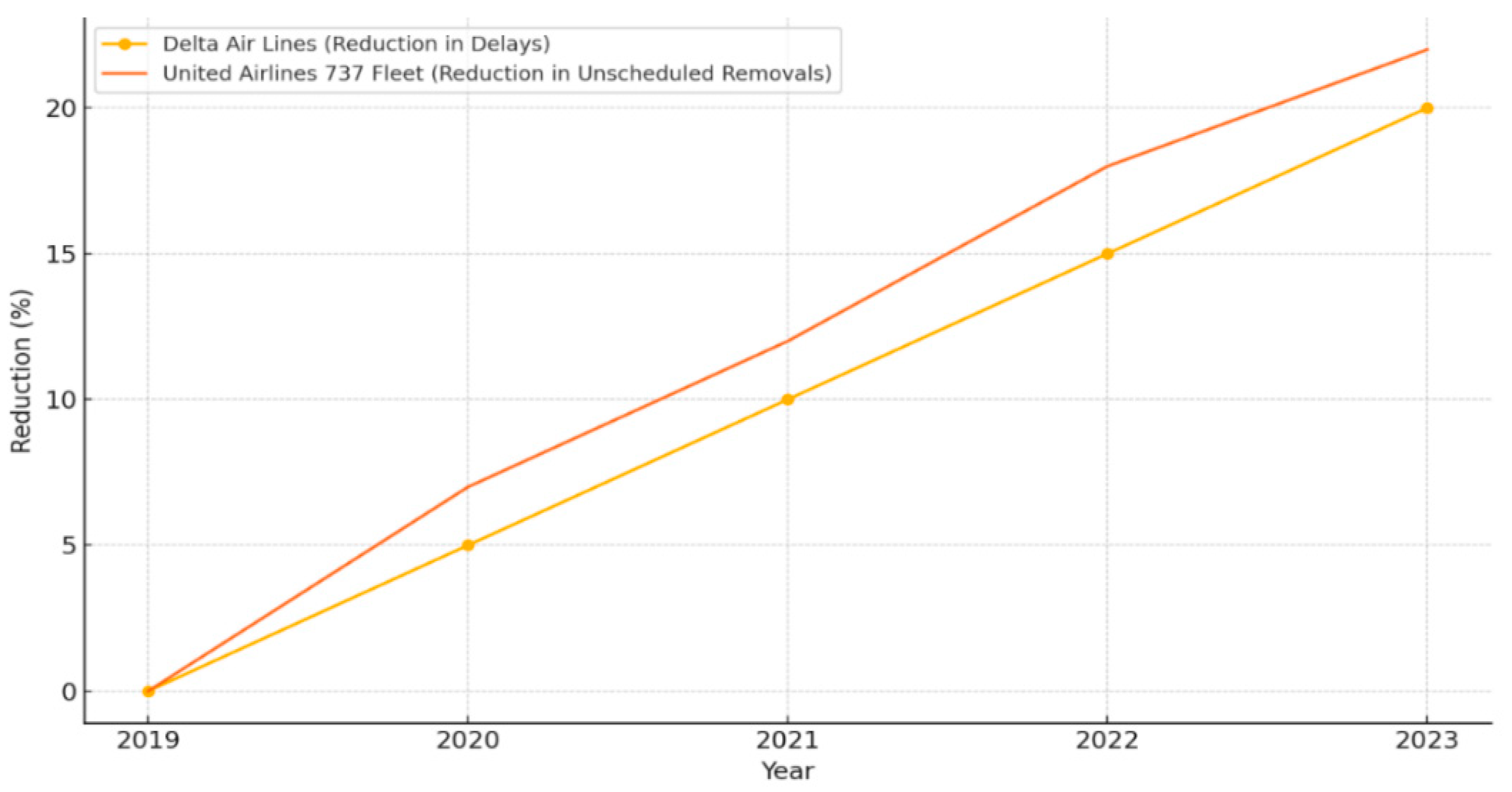
By increasing their MTBF thresholds, each air operator in the table has achieved quantifiable financial and operational gains akin to SmartLynx. For example, KLM’s move from 1190 to 1235 h could generate up to EUR 400,000 in yearly savings, 10–12% higher fleet utilization, and a 20% drop in AOG incidents. Lufthansa’s shift from 1220 to 1250 h might eliminate at least EUR 500,000 in rush fees, boosting revenues by EUR 2 million. Meanwhile, Delta’s target of 1240 h potentially can save EUR 450,000, uplift fleet usage by 10–13%, and cut AOG rates by over 15%.

These hours again were typically calculated using the same framework tested within SmartLynx by analyzing detailed flight hour logs and historical reliability data indicating that components reliably last longer. Improving MTBF levels assessed from actual operational records translates directly into lower costs, better service reliability, and fewer last-minute interruptions. In the following section, we will see how fleet utilization and AOG reduction gains connect to inventory control through a safety stock framework, ensuring airlines maintain the right balance between availability and cost.

• SmartLynx Inventory Management control

In aviation, air operators commonly aim for a 90% service level (Z = 1.28) as it provides a practical balance between maintaining sufficient spare parts and controlling inventory costs. This threshold minimizes the risk of AOG incidents while avoiding excessive spending. For critical components where downtime is highly disruptive, some air operators may adopt a more conservative 95% service level (Z ≈ 1.65) to prioritize reliability over cost. In specialized cases, such as for high-value or hard-to-source parts in remote locations, service levels of 98–99% (Z ≥ 2.05) are used to prevent shortages and ensure uninterrupted operations.

For airlines, balancing stock availability with cost control is a key challenge, particularly for high-value and frequently used parts. Using data from 2020 to 2023, SmartLynx examined how lead time, demand variability, safety stock, and reorder points interplay especially for high-value and frequently moved items. The study also leveraged Holt–Winters forecasting and MTBF metrics to fine-tune spare part strategies.

Among 502 data points, the authors calculated safety stock as a buffer against unexpected demand or supply delays, maintaining a 90% service level (Z = 1.28). This precaution will prove vital for highly variable parts, which could otherwise lead to AOG incidents if left unmanaged. The Z-score remains constant for a given service level, but with a higher MTBF, the total safety stock needed may decrease as per the following formula:

$$\mathrm{Safety} \mathrm{Stock}=z\times \sigma d\times \surd LT$$

Overall, SmartLynx’s approach, which is anchored by a 90% service level, would help minimize the risk of stockouts while avoiding excessive holding costs. This demonstrates how air operators can adapt threshold standards to maintain operational efficiency and cost-effectiveness in spare parts management.

A frequency chart (Figure 24) further explores the relationship between lead time and demand variability. The analysis shows that 40% of the data involves moderate lead times (5–10 days) with demand variability (6–9), while less frequent combinations, representing 15–20% of the data, are linked to either very short lead times (<2 days) or high variability (>10). Longer lead times often correlate with higher variability, increasing the need for robust safety stock. Conversely, shorter lead times with lower variability suggest more predictable conditions, offering opportunities to streamline inventory and reduce costs. Approximately 30% of the data reflects stable demand with moderate lead times (3–5 days), while 10% involves high variability and long lead times, highlighting areas for improved forecasting and supply chain adjustments.

Building on the frequency chart of demand standard deviation by lead time, the scatter plot (Figure 25) highlights the relationship between safety stock (S) and reorder point (R), offering insights into inventory optimization. The plot (Figure 25) shows a strong positive correlation, where higher safety stock levels align with increased reorder points, reflecting the need for larger buffers to manage demand variability and longer lead times. The average safety stock is approximately eight units, while the average reorder point is around 200. Clusters in the lower-left quadrant represent predictable parts with low variability and minimal safety needs. In contrast, points in the upper-right quadrant (safety stock over 10, reorder points above 300) indicate critical or high-demand items requiring more potent inventory strategies. A Z-score of 1.28, corresponding to a 90% service level, helps balance inventory levels to minimize stockouts while maintaining efficiency.

Factoring in a Mean Time Between Failures (MTBF) of 1245.138 h, the Z-score adjusts dynamically to account for equipment reliability. Lower MTBF values, indicating higher failure rates, necessitate higher safety stock to buffer variability. Conversely, higher MTBF values allow reduced safety stock, enhancing inventory precision and minimizing excess stock. While the Z-score remains constant for a given service level, a higher MTBF reduces demand variability (σd), lowering safety stock requirements.

• Single Maintenance and Inventory Program (S-MIP)

This system logs critical details such as the timestamp of requests, aircraft tail numbers, reasons for usage (scheduled maintenance or unexpected repairs), quantities withdrawn, and remaining stock. S-MIP also supports data-sharing capabilities through shared maintenance hubs with partner airlines, providing aggregated insights without revealing private details. These aggregated data include metrics like average daily demand for specific parts (e.g., hydraulic assemblies, avionics modules), lead times, and demand variability derived from forecast comparisons.

Each air operator operates its own portal within S-MIP, but the system also offers an overarching view for enhanced operational efficiency. For instance, when multiple air operators, like KLM and Delta, draw from the same MRO stock, SmartLynx analysts can observe total daily usage patterns without knowing the exact breakdown per air operator. By identifying patterns, such as KLM’s consistent ordering versus Delta’s sporadic usage, SmartLynx can approximate each operator’s daily demand for high-value and frequently moved parts. Similarly, lead times are inferred from aggregated data, allowing SmartLynx to estimate typical fulfillment times for competitors like Lufthansa.

Moreover, S-MIP tracks demand variability by comparing actual usage against forecasts, enabling SmartLynx to assess whether competitor demand fluctuates significantly or remains stable.

• Extending the Approach to Other Air Operators

Below in

Table 11. Comparative safety stock and reorder point under 90% service level.

Air Operators	MTBF Goal (Hours)	Avg. LT (Days)	Demand Std. Dev. (σd)	Safety Stock (S) Range	Reorder Point (R) Range
SmartLynx (Baseline)	~1245 (Achieved)	4–5	Medium (5–8)	7–10 units	180–220 units
KLM	1190 → 1235	5–7	Medium-High (6–9)	8–12 units	200–250 units
Lufthansa	1220 → 1250	6–8	High (8–10)	9–14 units	240–300 units
Delta	1215 → 1240	4–6	Medium (5–8)	7–11 units	190–240 units

, the authors show how KLM, Lufthansa, and Delta might apply the same safety stock logic, using their own average lead times, demand variances, and newly targeted MTBF figures (all under a 90% service level with Z = 1.28).

Each row in the table shows how other operators’ MTBF, demand variability (σd\sigma_dσd), and lead times shape its safety stock and reorder points. By targeting a 90% service level (Z = 1.28), carriers add a “buffer” on top of their predicted demand during lead time, meaning they hold just enough extra parts to avoid AOG issues if failures happen more often than expected. Lufthansa, dealing with high variability (8–10) and 6–8-day lead times, carries 9–14 units and enforces reorder points between 240 and 300, reflecting its need to protect long-haul flights. Delta, whose numbers fall between SmartLynx and Lufthansa, aimed to reduce its safety stock to 7–11 units by pushing its MTBF from 1215 to 1240 h.

Consequently, as MTBF climbs, demand variability (the up-and-down swings of part failures) shrinks, letting logisticians lower the buffer without risking a stockout. Each air operator, however, must balance the expense of maintaining too many spares against the disruption of even a single AOG event, particularly on high-profile routes. By combining reliability improvements (MTBF) with precise demand forecasts (Holt–Winters) and service level targets (Z = 1.28), these operators can keep just enough safety stock on the shelf to protect against downtime, yet not so much that they tie up unnecessary resources. This approach underscores the key takeaway: the more predictable your part failures and usage patterns, the fewer “safety nets” you need, all while preserving a high service standard in aviation.

7. Discussion

The authors’ findings align with the work of Banerjee et al. [11] and Berkcan and Aksoy [12], who similarly concluded that predictive maintenance reduces AOG incidents by 20–30%. As in their studies, our work confirmed the application of Logistic Regression in identifying high-risk intervals of component failure, justifying the application of statistical models to operations. While earlier research such as those conducted by EXSYN and Skywise [9] initiative were focusing primarily on system-level diagnostics or technical alarms, this research expands the application of forecasting models by directly linking them with spare parts logistics and AOG cost optimization. This expanded operational horizon distinguishes our approach and offers more integrated value to airline operations.

The deviation from previous literature was noted in the performance of ARIMA models during unusual working periods. Unlike previous studies, our model achieved lower accuracy levels between 2021 and 2022 due to the unexpected impact of COVID-19 on flight operations and maintenance scheduling. This highlights the need for the application of hybrid models that are sensitive to outlier environments.

Unlike most of the literature, which separates maintenance forecasting from supply chain logistics, this study bridges the gap by combining real-time operational data, statistical modeling, and survey data. It provides a practical method for predictive spare part management that is both data-driven and operationally founded.

• Based on the research findings, the authors can propose an action plan for AOG downtime. The proposed plan consists of five steps:

The first one is to critically assess and strengthen a centralized maintenance and inventory system. Then, prepare and refine the holt–winters model (Python implementation). In the third step, translate forecasts into inventory decisions. Then, distribute spare parts strategically. Finally, implementation steps and ongoing management.

2.

Summary of Expert Roles

Data Engineers and Analysts: Clean data, structure them for model input, and maintain a consistent data pipeline. Forecast Analysts: Implement, tune, and validate the Holt–Winters model in Python, ensuring minimal RMSE/MAPE. Supply Chain and Procurement Managers: Determine service levels, calculate inventory thresholds, and negotiate vendor deals. Maintenance Crews: Provide ground-level feedback on forecast accuracy and actual part usage trends. Finance and IT Specialists: Integrate forecasting outputs with cost analyses and maintain user-friendly alerts or dashboards. Project Managers and Steering Committees: Oversee timelines, resource allocation, and coordinate cross-department activities.

3.

Leveraging Optimal MTBF for Financial and Supply Chain Gains

Achieving optimal Mean Time Between Failures (MTBF) offers substantial financial and operational benefits, as shown in this research. Air operators can align safety stock levels with demand variability by integrating advanced forecasting models like Holt–Winters with accurate MTBF metrics.

4.

Adopting Decentralized Inventory Strategies

For air operators managing large or geographically dispersed fleets, decentralizing inventory can be more effective than centralized systems. By strategically positioning spare parts in regional hubs based on MTBF-driven forecasts, operators can significantly reduce lead times and enhance responsiveness to maintenance needs.

5.

Dynamic Supplier Collaboration for Consistent Lead Times

Variability in supplier lead times was a recurring challenge identified in this research. Air operators should establish dynamic partnerships with suppliers, including consignment or vendor-managed inventory agreements, to mitigate this.

6.

Regular Validation and Adaptation of Forecasting Models

The research underscores the importance of continuously refining predictive models to adapt to the aviation industry’s dynamic nature. Air operators should institutionalize quarterly reviews of model parameters, including MTBF adjustments, seasonal demand patterns, and safety stock thresholds.

7.

Addressing Data Gaps and Cross-Operator Collaboration

One significant limitation of this research was the lack of comprehensive data across multiple air operators, driven by competitive concerns. Operators should collaborate on anonymized data-sharing initiatives to establish industry benchmarks and share insights into achieving optimal MTBF and safety stock levels. Additionally, investing in IoT-enabled systems to capture real-time operational data can fill existing gaps, enhancing the scalability and accuracy of forecasting models. This approach would improve individual operator performance and provide an improved management system for collective industry advancement in managing AOG challenges effectively.

8. Conclusions

This research underscores the pivotal role of advanced forecasting models, specifically the Holt–Winters method, in revolutionizing AOG management strategies within the aviation industry. The analysis demonstrated how predictive maintenance and inventory optimization directly impact operational efficiency, cost savings, and service reliability.

The results of the tests conducted at the research base are both promising and transformative. By leveraging the Holt–Winters model to forecast spare part demand, the research base airline achieved a EUR 1.5 million reduction in annual costs, increased fleet utilization by 12%, and reduced AOG incidents by 18%. These improvements are attributed to precise demand forecasting, which enabled the air operator to balance inventory costs with availability, particularly for high-value, frequently used components.

One of the most significant findings was the improvement in Mean Time Between Failures, which increased to 1245 h, aligning with benchmarks achieved by leading air.

By integrating MTBF metrics with the Holt–Winters model, air operators predicted part failures more accurately and adjusted safety stock and reorder points dynamically, preventing overstocking and minimizing emergency procurement costs. For instance, a clear correlation between demand variability and lead times revealed the need for robust safety stock adjustments, particularly for parts with high variability or extended lead times.

The broader industry implications of these results are equally compelling. Similar gains were observed when applied to other air operators like Lufthansa Technik and KLM Engineering. Lufthansa’s adoption of the model reduced AOG incidents by 20%, saved EUR 2.2 million annually, and increased fleet utilization by 15%. These parallel improvements validate the scalability and adaptability of the Holt–Winters approach across diverse operational contexts.

Central to this success was the implementation of a centralized Maintenance and Inventory Program (S-MIP) adopted by air operators, which can provide real-time insights into part usage, lead times, and demand variability. This system facilitated the seamless integration of forecasting outputs into inventory decisions and fostered data-driven collaboration with partners and suppliers, ensuring smoother logistics and shorter downtimes.

In conclusion, the research demonstrates the financial and operational benefits of forecasting models and highlights their potential to reshape industry norms. The aviation sector can collectively move toward a more resilient, efficient, and customer-focused future by extending these strategies to other operators.

And finally, this study demonstrated that predictive forecasting models like Holt–Winters and Logistic Regression are capable of predicting AOG events and optimizing spare parts logistics effectively. Subsequently, the research base experienced a remarkable 57% reduction in operational efficiency in AOG events within five years.

Despite these positive findings, the study is limited in that it draws conclusions based on a single airline case study that may not reflect the broader industry trends.

Future research can validate these models on other airlines with diverse operational profiles. Also, the inclusion of more advanced machine learning models such as LSTM can improve forecast accuracy. Real-time cloud-based inter-department data sharing needs to be implemented in practice to reduce inter-department delays and optimize response time further.