1. Introduction
Wind power generation is a research hotspot in the field of renewable energy currently. As the installed capacity of wind turbines increases year by year, wind farms are gradually located closer to residential area, the noise generated by wind turbines during operation is an important issue to consider in design. The noise produced by wind turbines includes mechanical noise generated by the units and aerodynamic noise resulting from the interaction between the blades and the air. In the noise generated by megawatt-class large-scale wind turbines, the aerodynamic noise from the blades can exceed 90 dB, typically surpassing the mechanical noise [
1]. The airfoil noise is the root cause of wind turbine blade noise. Therefore, it’s necessary to study the noise predicted method of wind turbine airfoil. Common methods for calculating the aerodynamic self-noise of wind turbine airfoils include wind tunnel tests, BPM semi-empirical theory, and CFD.
Many researchers both domestically and internationally have conducted extensive studies on the noise generated by wind turbine airfoils. Christopher et al. [
2] investigated how changing the leading-edge shape of airfoils can reduce turbulent impact noise, proposing a solution that combines serrated edges with porous materials, which maintains good noise reduction effects while minimizing the impact on aerodynamic performance. Laura et al. [
3] studied the influence of airfoil geometric shapes on airfoil noise, using a phased microphone array to measure leading-edge and trailing-edge noise of different airfoil shapes at various chord lengths. Their paper established a noise prediction model based on airfoil geometry that accurately predicts airfoil noise and guides the noise reduction design of wind turbines. Irsalan et al. [
4] explored how to utilize distributed surface compliance to reduce airfoil noise, proposing a wing configuration based on distributed surface compliance that effectively reduces tonal noise across a wide range of angles of attack without negatively impacting aerodynamic performance. Wu Zhengren et al. [
5] employed Large Eddy Simulation (LES) and the FW-H analogy method to study the impact of ridge structures on the aerodynamic noise of the NACA0018 airfoil at a 6° angle of attack and different inflow velocities. The study indicated that arranging ridge structures in the adverse pressure gradient region can effectively reduce aerodynamic noise, particularly in suppressing low-frequency noise, thereby lowering pressure fluctuations and vortex intensity. Zheng Nan et al. [
6] utilized numerical simulation methods to compare and analyze the aerodynamic performance and noise characteristics of the NACA0018 airfoil equipped with Gurney flaps (GF) and serrated flaps (SGF), exploring the effects of tooth height and width on airfoil performance. They found that serrated flaps can significantly enhance the aerodynamic performance and noise reduction effects of wind turbine airfoils. Li Shoutu [
7] conducted numerical simulations using the ANSYS (2025 R1) Fluent platform, applying the LES turbulence model to calculate the flow field of the airfoil and the FW-H noise prediction model to determine the far-field noise characteristics of the airfoil, revealing the influence of geometric parameters on noise, providing important theoretical guidance for the design of VAWT airfoils and noise reduction technologies. The current research on airfoil noise remains predominantly reliant on conventional approaches, including geometric optimization, CFD simulations (e.g., LES) combined with acoustic analogy methods (e.g., FW-H). While these methods demonstrate their maturity, they have long computation times and require significant computational resources. In light of the challenges posed by the increasing scale of wind turbines and associated nonlinear noise amplification, there is an urgent need to integrate interdisciplinary technologies such as AI-driven design to develop innovative noise prediction.
In recent years, deep learning has rapidly developed across various fields [
8]. Based on artificial neural networks, deep learning employs a multi-layered network structure for feature learning and pattern recognition. The key lies in training the network model to extract data features, enabling efficient classification, regression, and generation tasks. Researchers both domestically and internationally have made progress in applying deep learning to the study of wind turbine and airfoil noise.
Xiao Chunhua et al. [
9] proposed a novel ice thickness detection method based on changes in the far-field noise of iced airfoils, establishing a multivariable input neural network prediction model that can predict the maximum ice thickness based on flight parameters and total sound pressure level increments, effectively improving the accuracy and reliability of ice detection. Han Yang et al. [
10] introduced a method utilizing convolutional neural networks (CNN) and a specialized airfoil noise database to predict the noise of wind turbine airfoils. This model effectively predicts the noise generated by wind turbine airfoils and serves as an effective tool for assessing airfoil noise and designing low-noise blades, achieving a high prediction accuracy with a Mean Absolute Percentage Error (MAPE) of less than 0.0531%. Altice et al. [
11] constructed a new dataset named CAI-SWTB using deep learning algorithms, employing five basic CNN architectures for wind turbine blade fault detection and exploring transfer learning techniques. The transfer learning Xception model achieved an accuracy of 99.92% on the CAI-SWTB dataset. Stéphane et al. [
12] developed a prediction model based on deep neural networks (DNN) to more accurately predict airfoil self-noise, especially turbulent boundary layer trailing edge noise, using NASA’s experimental noise dataset for training. Their research concluded that the DNN model is an effective and accurate tool for predicting TBL-TE noise, and further studies revealed that the DNN model can uncover the physical mechanisms behind TBL-TE noise, providing more guidance for airfoil design and noise reduction technologies. The aforementioned studies demonstrate the applicability of deep learning techniques, particularly CNN, in airfoil/blade identification and noise characterization. The image recognition capabilities of CNN align well with the structural feature extraction requirements in this study, enabling effective pattern recognition of airfoil noise sources and flow-acoustic coupling mechanisms. This methodology provides a robust framework for data-driven noise prediction and optimization in our research.
Currently, researchers both domestically and internationally commonly use wind tunnel tests, BPM semi-empirical theories, and CFD methods to calculate the aerodynamic noise of wind turbine airfoils. However, there is relatively little research on the application of deep learning techniques for predicting airfoil noise. This field faces challenges such as a limited existing database of wind turbine airfoils [
9], large computational demands for noise prediction, and low efficiency.
To solve these problems, this paper presents an airfoil noise prediction model based on a generalized airfoil set and deep learning. A generalized airfoil dataset with rich curvature, thickness, and trailing edge features can be generated based on common 31 kinds of airfoil shapes. The airfoil integrated theory; B-spline function and CST method are introduced to express the common airfoils, which makes the airfoil dataset more comprehensive. This approach aims to enhance the generalization ability of deep learning models in the field of wind turbine noise prediction. The generated dataset is then used to train the ResNet18 model, which is compared with other common machine learning models to validate its performance and investigate its computational efficiency.
2. Generation and Representation of Generalized Airfoil Set
The dataset is a key component of deep learning, and the performance of deep learning models is influenced by the dataset. The more diverse and larger the deep learning dataset, the stronger the generalization ability and higher the prediction accuracy of the deep learning model [
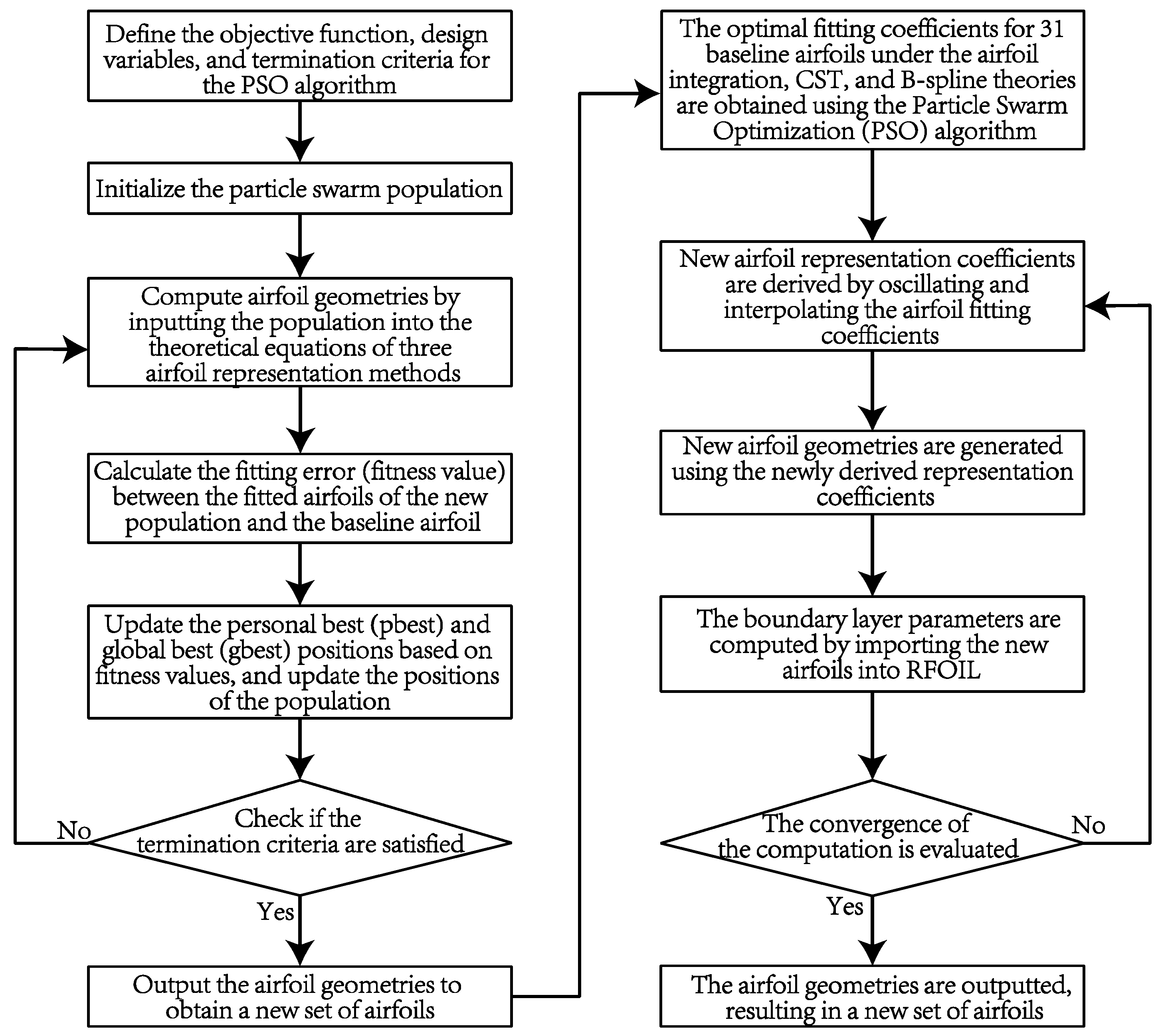
13]. This section first fits the basic airfoils based on airfoil integration theory, CST theory, and B-spline theory, and obtains optimal fitting parameters through a particle swarm optimization algorithm. The obtained fitting parameters are then subjected to oscillation, interpolation, and other operations to generate the generalized airfoil set.
To enrich the generalized airfoil set, this paper used 31 basic airfoils with different thicknesses, camber, and trailing edge geometrical features from the NACA, DU, FFA, RISO, and other series to generate new airfoils. These basic airfoils are all airfoils commonly used in wind turbine blade designs. The generation process of the generalized airfoil set is illustrated in
Figure 1.
2.1. Airfoil Integration Theory and Its Airfoil Set Generation
The Joukowski transformation can convert a circular arc into an airfoil [
14]. The circular arc is defined in the z-plane, with the center coordinates at (−ε1, ε2) and a radius of
r. Through the Joukowski transformation, it can be transformed into an airfoil in the ζ-plane. The formula in the ζ-plane is as follows:
In the equation, a represents one-fourth of the airfoil chord length. The coordinates of any point on the circular arc can be expressed as z = r·exp(iθ), and r and z are represented by the following formulas:
From the above equation, it can be seen that z is a function of θ, and different functions ϕ(θ) can yield different airfoil shapes. Based on the Joukowski transformation theory, the generalized functional equation for ϕ(θ) can be expressed as follows:
By setting different values for parameters
a and
b in Equation (4), various airfoil shapes can be obtained. During the airfoil fitting process, determining the appropriate values of
a and
b is particularly critical. In this study, the optimal airfoil fitting parameters are obtained through iterative computation using the PSO algorithm. The coefficients
a and
b in the theoretical airfoil integration formula Equation (4) are treated as design variables, while the mean square error (MSE) of the
y-coordinate values between the fitted airfoil and the original airfoil at selected chordwise positions serves as the objective function. However, when simultaneous fitting of the upper and lower surfaces is applied, certain airfoils with larger camber exhibit noticeable deviations between the fitted and original airfoil shapes, as shown in
Figure 2.
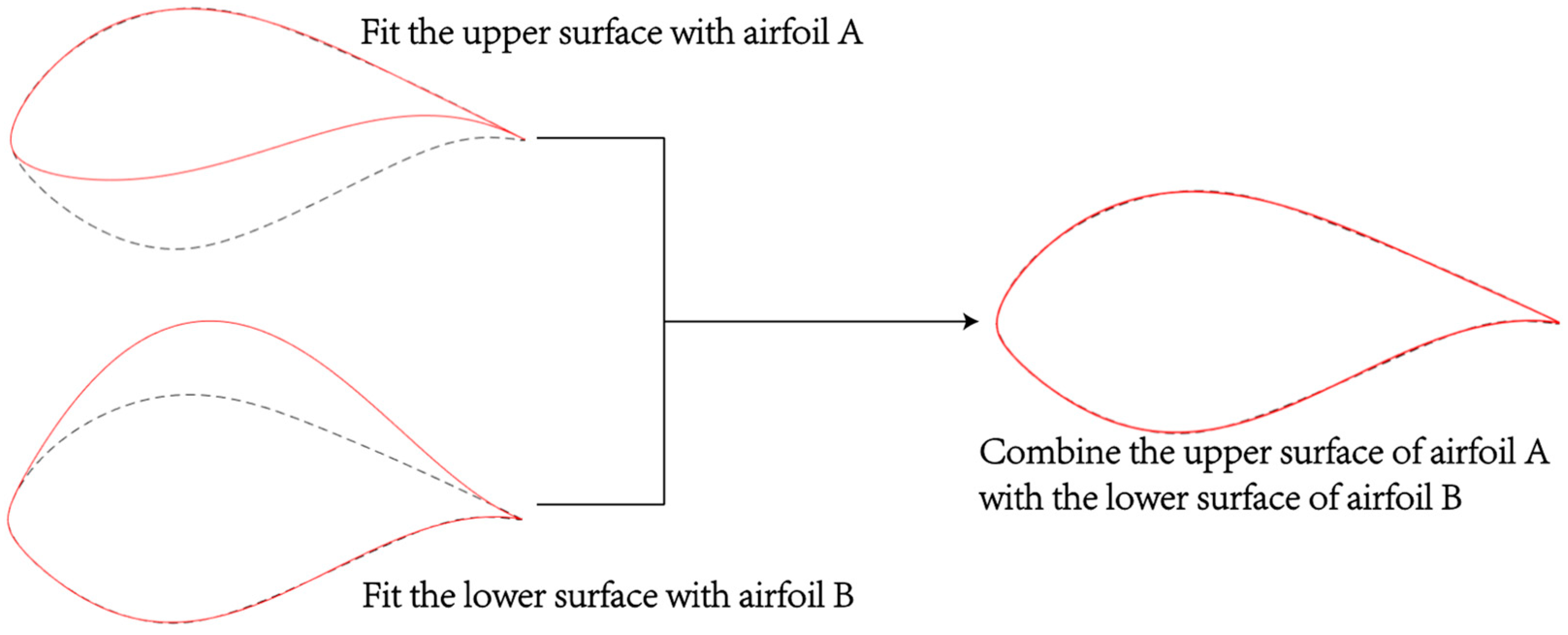
To address this problem, this study employs the airfoil integration theory combined with the PSO algorithm to fit the upper and lower surfaces of a baseline airfoil separately. The fitted upper and lower surfaces are then combined, as illustrated in
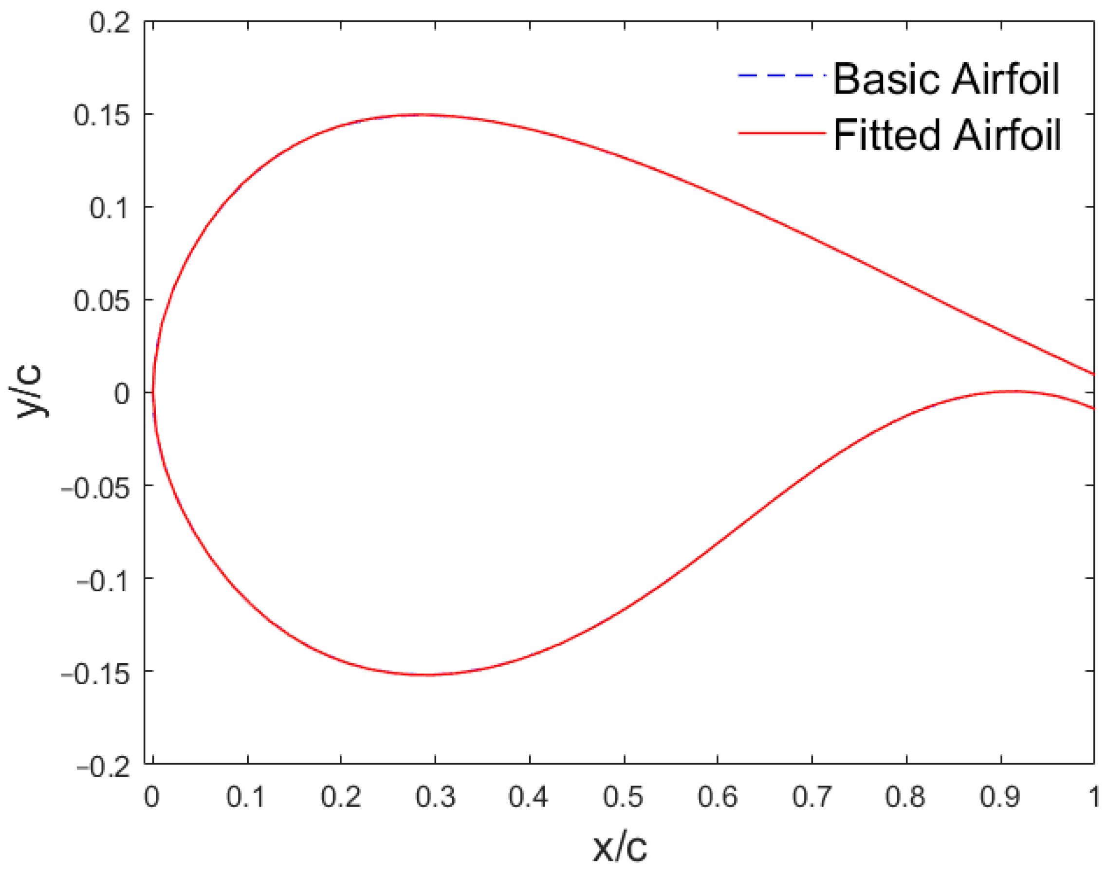
Figure 3. In the PSO algorithm, two distinct populations are established: Population 1 fits the upper surface, while Population 2 fits the lower surface. These two populations iterate independently, with their respective objective functions defined as the mean square error of the y-coordinate values of the upper and lower surfaces at selected chordwise positions. During the optimization process, an inertia weight decay strategy is implemented to progressively enhance the fitting accuracy. Each time the iteration count reaches a specified step length for inertia weight reduction, the inertia weight is multiplied by a predefined decay factor. The optimization algorithm was used to fit the airfoil to obtain the optimal coefficients of fitting the upper and lower airfoil surfaces respectively, and then the optimal upper and lower airfoil surfaces were combined to obtain the final fitting airfoil. The PSO algorithm parameters are listed in
Table 1, and the fitting results are presented in
Figure 4. The results demonstrate that this method effectively fits the baseline airfoil and yields the corresponding fitting parameters.
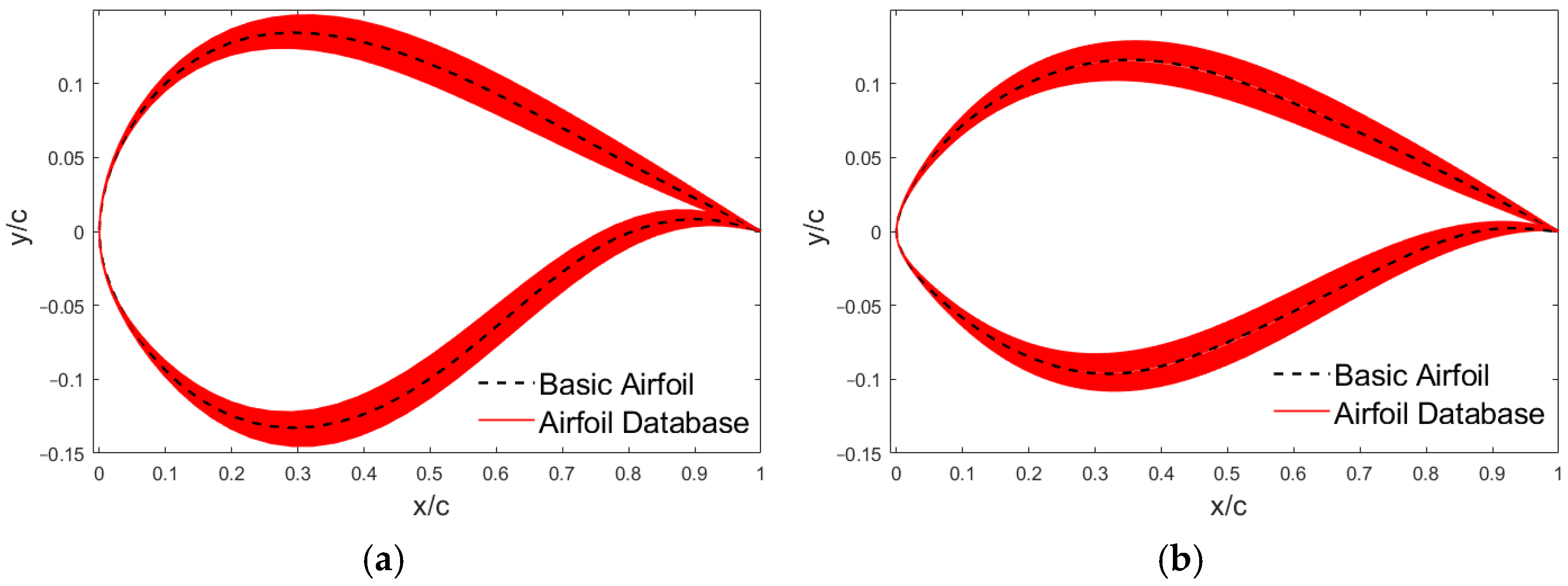
When utilizing the airfoil integration theory to generate a series of airfoils, the fitting parameters obtained in the previous step can be perturbed within a certain range, resulting in airfoils with varying camber and thickness characteristics. This approach provided a method for generating airfoils with different camber and thickness profiles based on a baseline airfoil. Once the new airfoil representation parameters are obtained according to Equation (5), the new airfoil profiles can then be generated using these updated parameters.
In the formula: P represents the parameters a and b in Equation (4).
Using this method, the airfoil set shown in
Figure 5 can be obtained.
2.2. CST Theory and Its Airfoil Set Generation
The Class function/Shape function Transformation (CST) method is a technique proposed by Kulfan and colleagues from Boeing [
15]. The upper and lower surfaces of an airfoil are expressed using the following two formulas:
In the equations: ψ—the dimensionless x-coordinate of the airfoil, ψ = x/c; ζ—the dimensionless y-coordinate of the airfoil, ζ = z/c; ΔξUpper—the leading-edge thickness ratio of the upper surface, ΔξUpper = zuTE/C; ΔξLower—the trailing-edge thickness ratio of the lower surface, ΔξLower = zlTE/C.
The class function is defined as follows:
The shape function
S(
ψ) is defined as follows:
In the equations: Vui, Vli—Coefficients of the shape function components for the upper and lower surfaces of the airfoil; Si(ψ)—Bernstein polynomials; n—Order of the Bernstein polynomials for the upper and lower surfaces of the airfoil.
When fitting the baseline airfoil using the CST theory, the PSO algorithm is employed to determine the fitting parameters. The design variables include the shape function coefficients
Vu,
Vl, as well as the parameters
N1 and
N2 from CST theory. The mean squared error of the
y-coordinate values between the fitted airfoil and the original airfoil at selected chordwise positions is used as the objective function. The algorithm parameters are provided in
Table 1, and the fitting performance is shown in
Figure 6. The results indicate that this method effectively fits the baseline airfoil and yields the corresponding fitting parameters.
To enrich the airfoil set with more diverse geometric features, interpolation methods are utilized to generate interpolated airfoils based on two baseline airfoils created using the CST method. By applying the aforementioned optimization algorithm to fit the two airfoils, two sets of shape function coefficients and
N1,
N2 values can be obtained. The parameterization formula for the interpolated airfoil is expressed as follows:
In the formula: QA, QB—represent the fitting parameters of the two baseline airfoils, where Q = [Vu, Vl, N1, N2]. Here, Vu and Vl are the shape function coefficients described in Equations (9) and (10), while N1 and N2 are the parameters defined in Equations (6) and (7).
Using this method, a set of airfoils with intermediate characteristics between any two airfoils can be obtained, as illustrated in
Figure 7. This approach allows interpolation both within the same airfoil family and across different airfoil families, resulting in an enriched set of airfoils with more diverse geometric features.
2.3. B-Spline Theory and Airfoil Set Generation
B-spline theory is widely applied in airfoil parameterization and optimization tasks [
16]. The B-spline function is expressed as follows:
where
Pk,n(
t) represents the
k-th segment of the
n-degree B-spline curve, and
Pi (
i = 0, 1, …,
n +
m) are the vertices of the B-spline characteristic polygon.
The expression for the basis function
G(
t) is as follows:
For a cubic B-spline curve, the basis function expression becomes:
The matrix form of the cubic B-spline function is given as:
where
P0,
P1,
P2,
P3 are the control points, and
t represents the horizontal coordinate of the B-spline curve. In this study, the airfoil is expressed by positioning control points on the airfoil curve. By setting different control points
P, various airfoil geometries can be obtained.
The process of fitting the baseline airfoils using B-spline theory is illustrated in
Figure 1, with the relevant parameter design provided in
Table 1. The fitting results, as shown in
Figure 8, demonstrate that the method accurately fits the baseline airfoils and extracts the corresponding fitting parameters.
Similar to the airfoil interpolation method using CST theory, the fitting of two airfoils using the above optimization algorithm yields two sets of control point coordinates. After obtaining the new control point coordinates using Equation (17), the new airfoil is generated from these new control points.
where
KA and
KB represent the control point coordinates of the two baseline airfoils. The process of fitting the baseline airfoils using B-spline theory is illustrated in
Figure 1, with the relevant parameter design provided in
Table 1. The fitting results, as shown in
Figure 8, demonstrate that the method accurately fits the baseline airfoils and extracts the corresponding fitting parameters.
Using this method, a set of airfoils with intermediate characteristics between any two airfoils can be obtained, as illustrated in
Figure 9.
In order to enrich the airfoil dataset as much as possible, the above three expression are used to generate new airfoils. The sharp trailing edge airfoils with different bend and thickness characteristics are generated by the airfoil integrated theory. Also, some new airfoils are generated by the interpolation method based on CST and B-spline theory. A program is made by using MATLAB(R2023a) software to generate airfoil datasets.
When calculating airfoil noise, the RFOIL software is used to compute the boundary layer parameters of the airfoil [
17]. To ensure that the airfoil set successfully converges during RFOIL calculations, each newly generated airfoil is imported into RFOIL for calculation. If the calculation fails to converge, the airfoil is regenerated until successful convergence is achieved, ensuring that each new airfoil serves as valid input data for noise calculations.
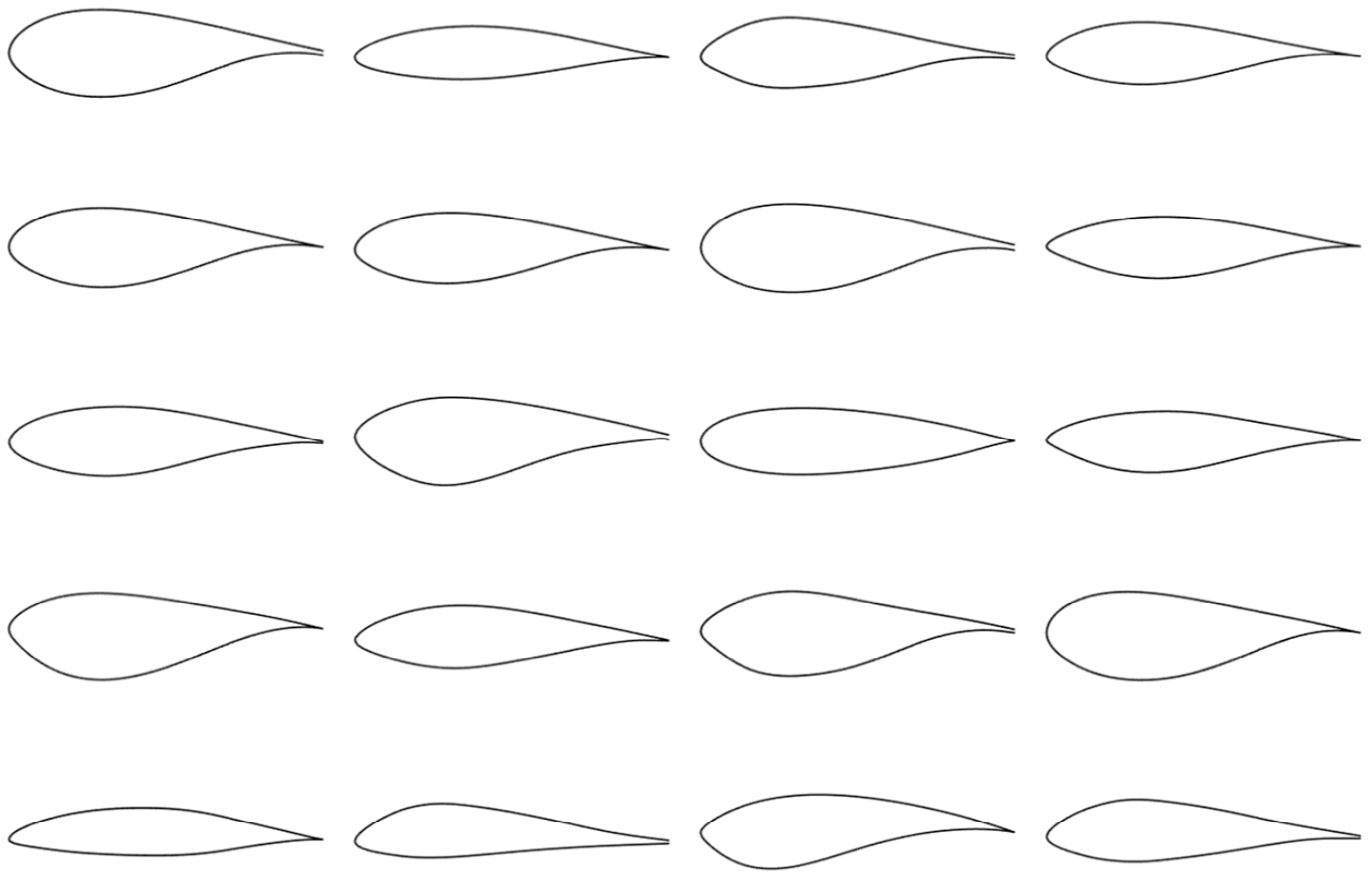
Using the above method, a generalized airfoil set containing 18,300 airfoils was generated. Each airfoil was subsequently converted into airfoil images with a resolution of 320 × 180 pixels, as shown in
Figure 10.
3. BPM Theory and Noise Label Set Generation
Airfoil self-noise originates from the trailing edge of the airfoil and is one of the primary sources of aerodynamic noise in wind turbine blades, caused by instabilities within the boundary layer flow on the airfoil surface [
18,
19]. According to the classical BPM model, airfoil self-noise consists of five components:
In the equations: SPLp—pressure surface noise, SPLs—suction surface noise, —Thickness of the boundary layer at the trailing edge of the suction and pressure surfaces, St—Strouhal number, GA—noise spectral shape function, W1—trailing edge noise amplitude function; ΔW1—sound pressure level correction function, Δl—the spanwise length of the airfoil.
- 2.
Separated Flow Stall Noise (SEP)
In the equations: GB—Stall noise spectrum shape function, W2—Stall Noise Amplitude Function.
- 3.
Laminar Boundary Layer Vortex Shedding Noise (LBL-VS)
In the equations: The shape functions G1, G2, and G3 are respectively dependent on the Reynolds number, Strouhal number, and angle of attack.
In the equations: Mmax—Maximum mach number in the area of tip vortex formation, —The modified Stouhal number, ltip—The span-wise extension of the tip vortex at the trailing edge.
- 5.
Trailing Edge Bluntness Vortex Shedding Noise (TEB-VS)
In the equations: h—Trailing Edge Thickness, G4—Spectrum at peak levels, G5—An auxiliary function for adjusting the shape of the spectrum.
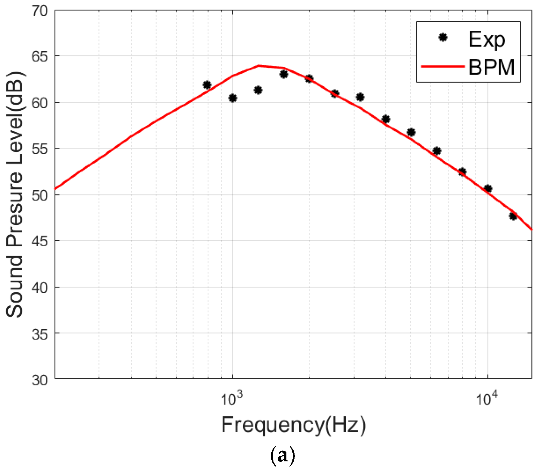
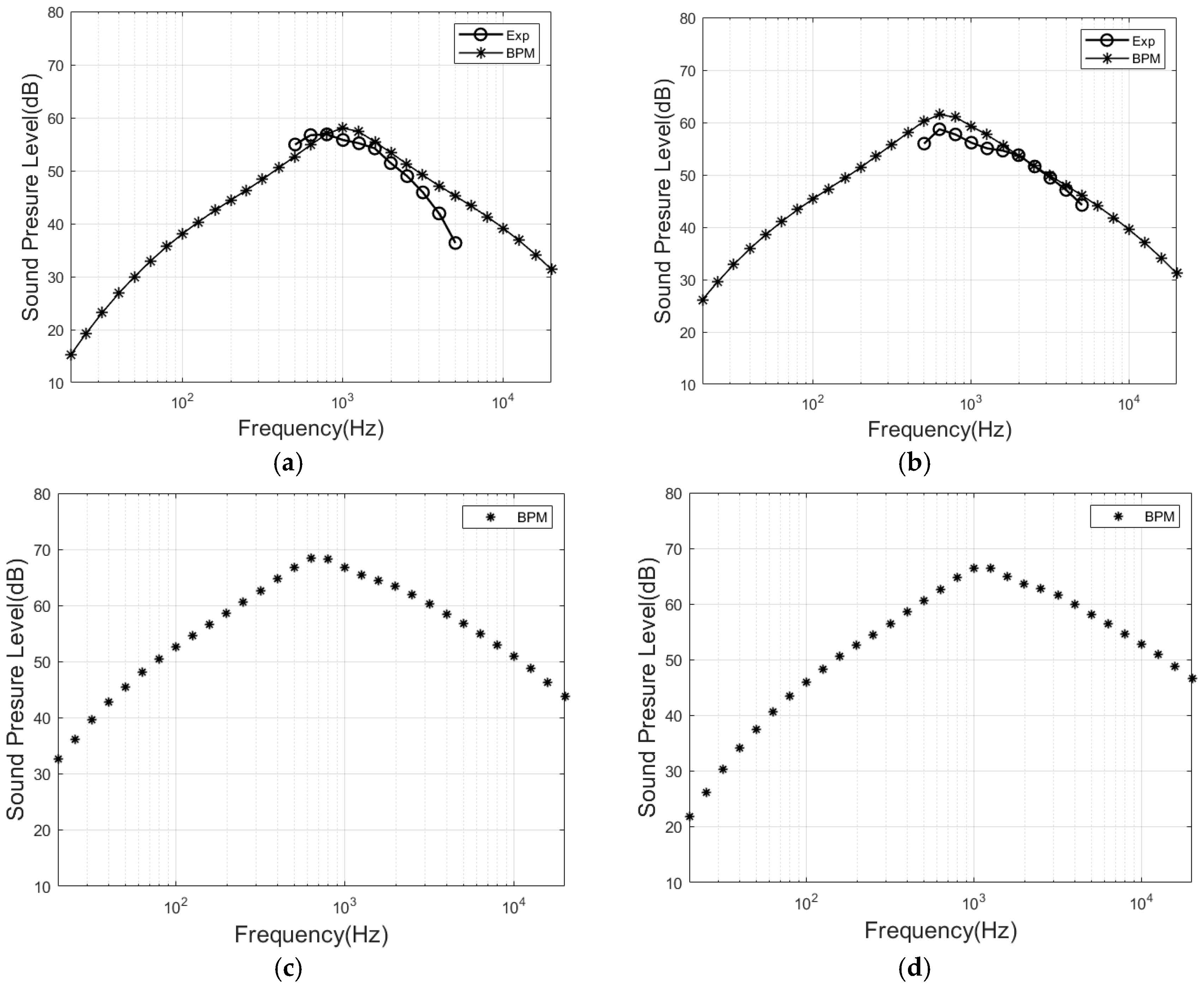
To verify the reliability of the BPM theory in predicting the self-noise of wind turbine airfoils, the prediction accuracy of the NACA0012 airfoil noise was evaluated by combining the BPM model with experimental data. When calculating the self-noise of the airfoil, the chord length was set to 30.48 cm, the observation angle was set to 90°, the observer distance was set to 1.22 m, the incoming wind speed was 71.3 m/s, and the angles of attack were set at 0°, 10.8°, and 14.4°. We used MATLAB together with the RFOIL program as a tool for calculating noise. The results are shown in
Figure 11.
By comparing the BPM predicted spectrum with experimental data, it can be seen that the results from BPM theory agree well with the experimental data, although there is a slight deviation below 2000 Hz. This model can be used to generate two-dimensional airfoil noise data in subsequent research, thereby enabling training for deep learning models.
Due to the strong agreement between noise predictions from the semi-empirical BPM model and experimental data [
20], this section uses the BPM semi-empirical model to calculate the noise for the generalized airfoil set. The resulting airfoil noise data serve as the label set for training the neural network and correspond one-to-one with the generalized airfoil set. The calculation procedure is as follows:
RFOIL is employed to calculate the aerodynamic performance of the generalized airfoil set and to extract the boundary layer parameters relevant for noise calculations. The calculation conditions are set as Re = 6.0×10⁶ and Ma = 0.15.
The boundary layer parameters extracted in the previous step are input into the BPM model to compute the noise levels (in decibels) across 31 frequency points ranging from 20 Hz to 20,000 Hz. The calculation conditions are specified as follows: Relative wind speed: 70 m/s; Observation distance: 1 m; Observation angle: 90°; Airfoil chord length: 1 m; Airfoil span: 0.5 m.
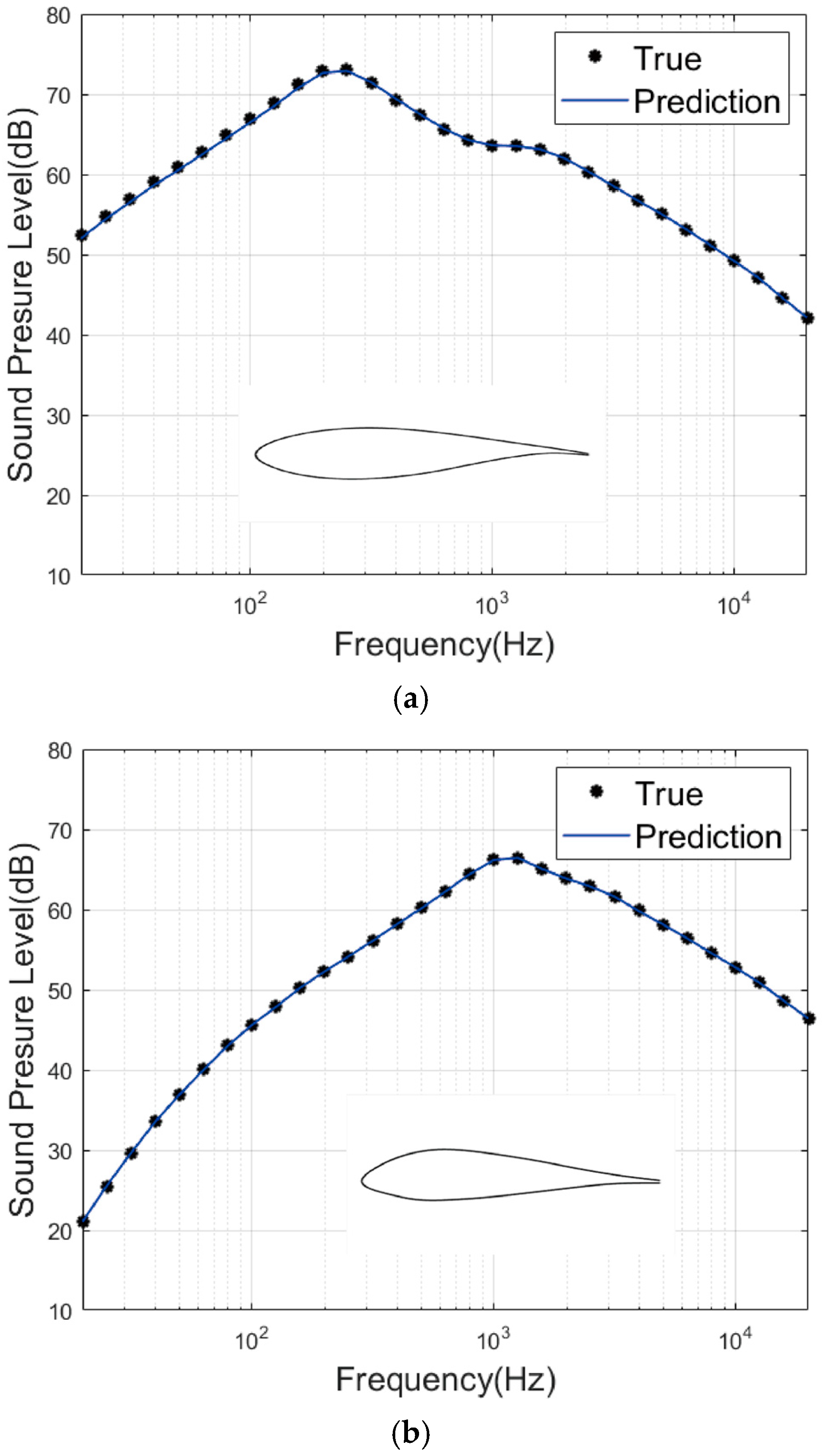
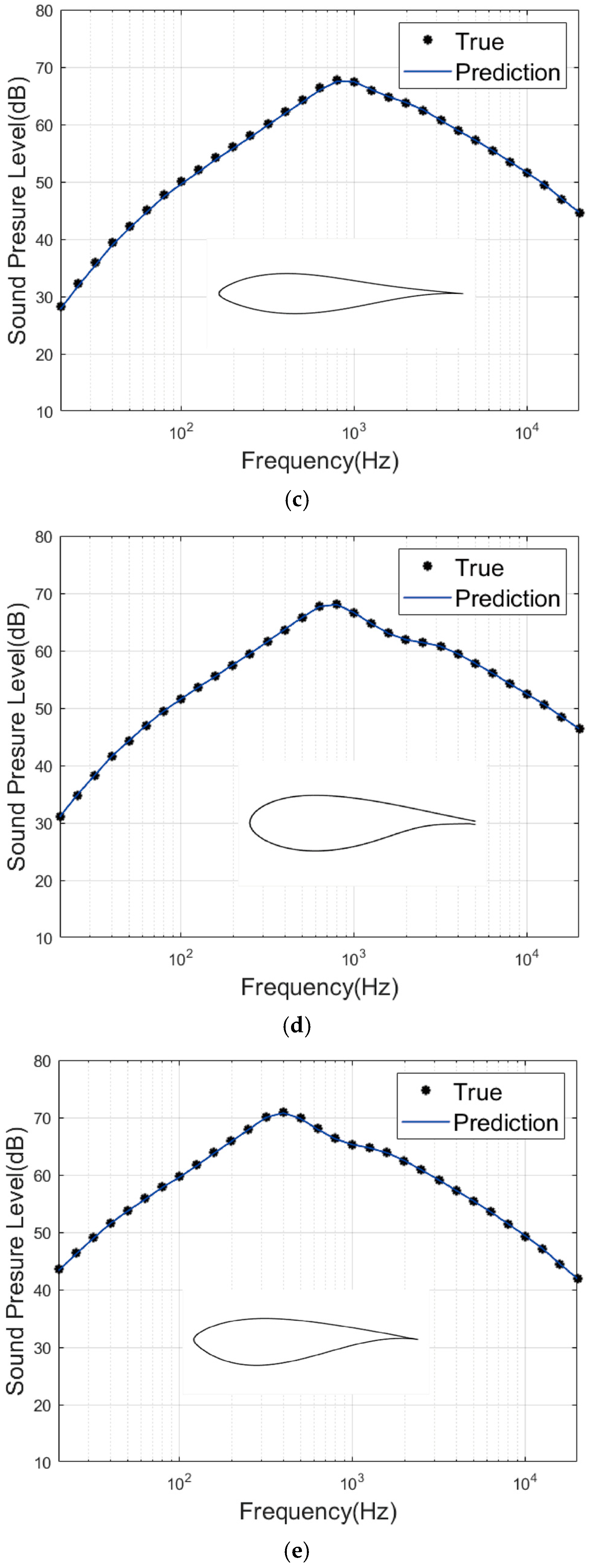
Upon completion, 18,300 sets of noise data are obtained, as illustrated in
Figure 12. As shown in
Figure 12a,b, the noise characteristic calculated by BPM theory agree well with the experimental data.
4. Airfoil Noise Prediction Model Construction
A Convolutional Neural Network (CNN) [
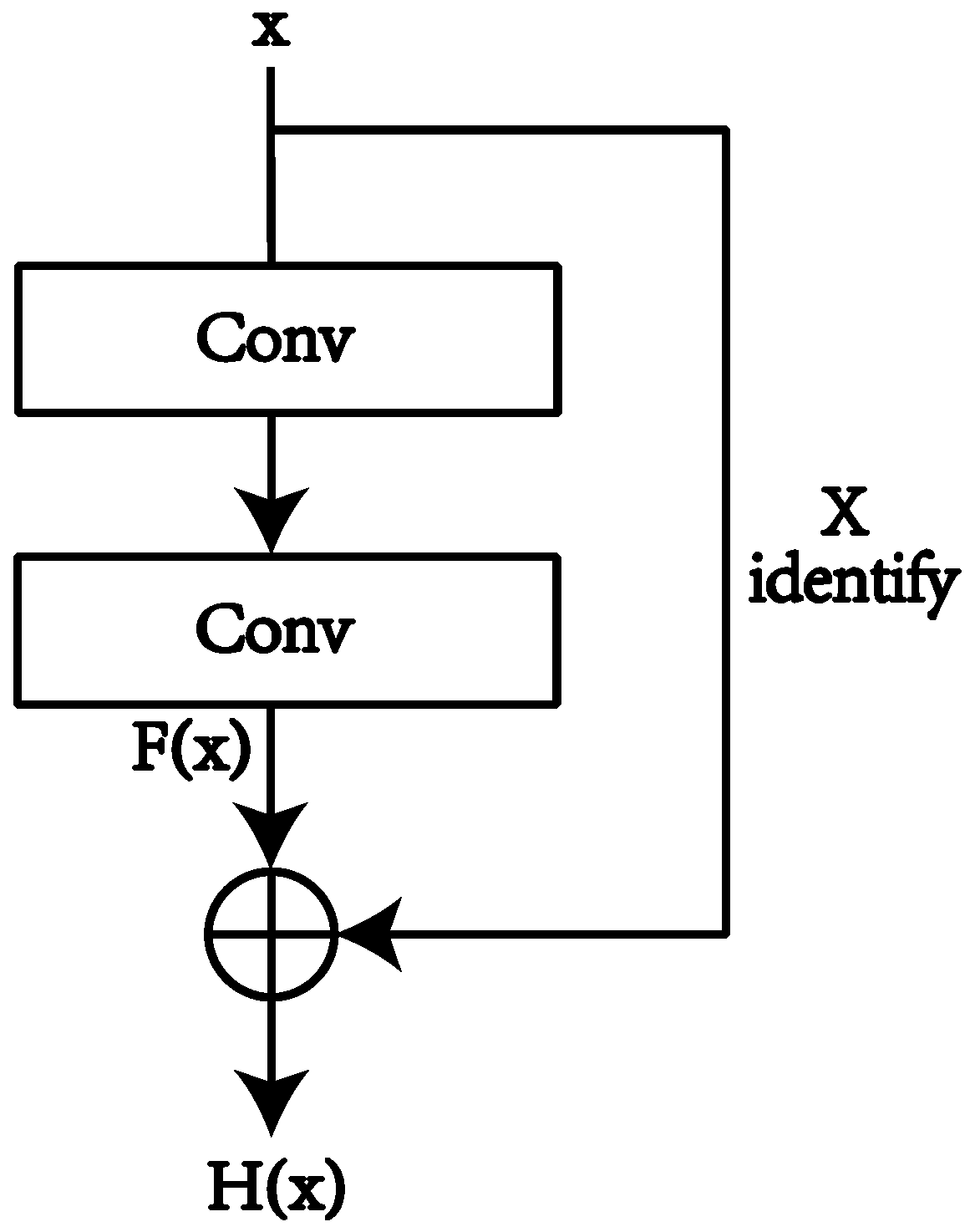
21] is a specialized neural network designed to process grid-structured data. CNNs excel at extracting features from grid-based datasets and are widely used in fields such as object recognition, speech recognition, and image recognition. For this study, CNNs are employed to identify airfoil data. However, traditional CNN models face limitations as their depth increases, particularly due to gradient vanishing or gradient explosion issues during training in deep neural networks. Residual Neural Networks (ResNet) [
22,
23] effectively overcome these limitations. As shown in
Figure 13, ResNet introduces residual connections to the standard CNN structure. The model’s objective during training is to learn the residual function
F(
x) =
H(
x) −
x. When
F(
x) = 0, it implies
H(
x) =
x, which corresponds to an identity mapping. Residual connections allow the output of one layer to bypass several intermediate layers and connect directly to a subsequent layer’s input, effectively mitigating the gradient vanishing or exploding problems. The output and input relationship can be expressed as:
where:
H(
x) represents the final output, and
F(
x) is the result of operations such as convolution and pooling.
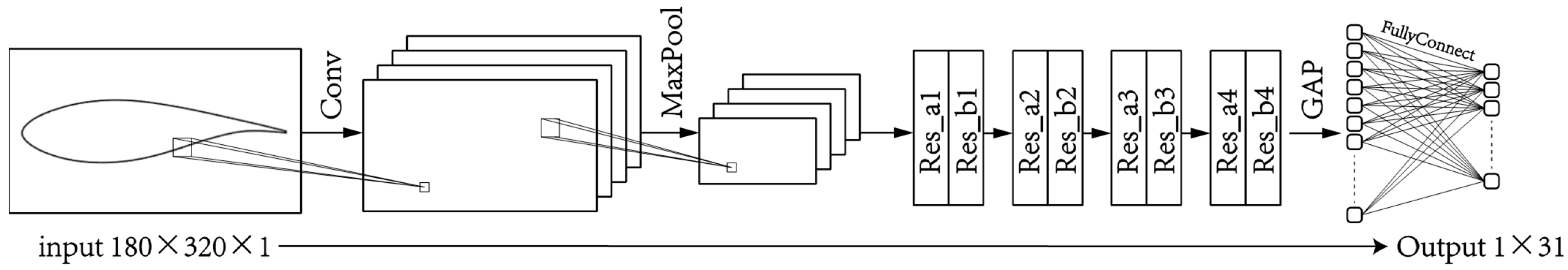
In this study, a wind turbine airfoil noise prediction model is constructed using the ResNet-18 architecture. The model structure is illustrated in
Figure 14. The input layer consists of two-dimensional airfoil data. After initial convolution and pooling operations, the data are passed through the residual blocks of ResNet-18. Subsequently, a Global Average Pooling (GAP) layer processes the data into a one-dimensional form. The output layer is then connected, where the number of neurons is set to 31, corresponding to the number of frequency points in the noise label set. The parameters of the ResNet-18 structure are detailed in
Table 2. The framework to build the deep learning models is provided by MATLAB’s deep learning toolbox.
As shown in
Figure 15, each airfoil image is digitized into a two-dimensional matrix, where each pixel corresponds to a parameter in the matrix. Noise data for each airfoil, obtained via BPM theory, are transformed into a 1 × 31 vector. Thus, each airfoil and its corresponding noise data are converted into a format suitable for training the neural network model.
The dataset comprises 18,300 samples, where:14,640 airfoils and noise data are used as the training set 1830 airfoils and noise data are used for validation during training, and 1830 airfoils and noise data are used as the test set. The ratio of the number of samples in the training set, validation set, and test set is 8:1:1.
The data were split using a random division method. Both the two-dimensional airfoil matrix data and the noise data were preprocessed using linear normalization to enhance computational efficiency.
During ResNet-18 model training, the Stochastic Gradient Descent with Momentum (SGDM) algorithm is used for optimization. The training settings include: Batch size: 80, Max Epochs: 1200, Learning rate: 0.006, Learning rate decay factor: 0.5 (learning rate decreases every 240 epochs), Validation frequency: 5000 iterations, Validation patience: 20 epochs.
This framework effectively processes airfoil data and corresponding noise vectors, leveraging the ResNet-18 architecture to improve the accuracy and robustness of noise prediction. The above data processing work is completed in MATLAB.
5. Airfoil Noise Prediction Model Validation
To verify the feasibility and superiority of ResNet-18 in airfoil noise prediction, a comparative analysis was conducted between ResNet-18, Random Forest (RF) [
24], Long Short-Term Memory (LSTM) [
25] networks, traditional CNN, and ResNet-50. Mean Squared Error was used as the loss function to quantify the error between actual and predicted values. Additionally, the coefficient of determination (
R2) was adopted as a key evaluation metric, as it quantifies the correlation between predicted and actual values in regression models. The formulas for MSE and
R2 are:
After training, the performance of the five models on the test set is summarized in
Table 3. While all models performed well in airfoil noise prediction, ResNet-18 and ResNet-50 exhibited the best
R2 and MSE values. Among these, ResNet-18 achieved the highest
R2 and the lowest MSE, demonstrating the most accurate prediction performance.
Table 3. shows the computation times of these models, where the random forest is the fastest, ResNet-50 is the slowest, and ResNet-18 has a speed in between; however, the differences in computation time between the models are actually very small. Considering the computational accuracy and speed of each model, the ResNet-18 model is the best choice. The relationship between predicted and actual values for ResNet-18 on the test set is depicted in
Figure 16. Ideally, if predicted values perfectly match actual values, data points would align along the diagonal. In the figure, the data points closely approximate the diagonal, confirming the high prediction accuracy of ResNet-18.
As shown in
Figure 17, the overlap between predicted and actual noise values for the test set at a frequency of 1000 Hz is highly pronounced, indicating excellent prediction accuracy. Similarly,
Figure 18 illustrates the relationship between predicted and actual noise frequency spectra across 31 frequency points ranging from 20 Hz to 20,000 Hz for random test samples. The predicted and actual values are nearly identical at all frequency points, further validating the high precision of the ResNet-18 model.
To evaluate the efficiency of the neural network in airfoil noise prediction, the computational time of ResNet-18 was compared with that of BPM theory, The computational time of the BPM model considers the parameters obtained using RFOIL. As summarized in
Table 4, ResNet-18 required approximately 0.0457 s to compute airfoil noise, while BPM theory required approximately 0.8 s. This indicates that the computational speed of ResNet-18 has improved by 94.3% compared to BPM theory.
6. Conclusions
To enhance prediction accuracy, generalization capability, and computational speed in wind turbine noise prediction, this study proposed a novel airfoil noise prediction model based on generalized airfoil sets and ResNet-18. Using Airfoil Integration Theory, CST theory, and B-spline theory, a generalized airfoil set with rich geometric features was generated. The corresponding noise data were computed using BPM theory, resulting in a dataset containing 18,300 samples with strong generalization capability.
This dataset was used to train the ResNet-18 model and compared against Random Forest, LSTM, traditional CNN, and ResNet-50. The results indicate that all five models performed well on the test set, but ResNet-18 outperformed the others, achieving an R2 of 0.99972 and an MSE of 0.0282.
This model provides a valuable reference for regression-based prediction of airfoil characteristics in other contexts and can be extended to the study of three-dimensional wind turbine blade noise prediction using deep learning techniques.


