Article

Quantum Snowflake Algorithm (QSA): A Snowflake-Inspired, Quantum-Driven Metaheuristic for Large-Scale Continuous and Discrete Optimization with Application to the Traveling Salesman Problem

1
Faculty of Engineering, Electrical and Electronics Engineering Department, Nuh Naci Yazgan University, 38170 Kayseri, Türkiye
2
Faculty of Economics and Administrative Sciences, Nuh Naci Yazgan University, 38170 Kayseri, Türkiye
*
Author to whom correspondence should be addressed.
These authors contributed equally to this work.
Appl. Sci. 2025, 15(9), 5117; https://doi.org/10.3390/app15095117
Submission received: 1 April 2025 / Revised: 25 April 2025 / Accepted: 29 April 2025 / Published: 4 May 2025

Abstract

:
The Quantum Snowflake Algorithm (QSA) is a novel metaheuristic for both continuous and discrete optimization problems, combining collision-based diversity, quantum-inspired tunneling, superposition-based partial solution sharing, and local refinement steps. The QSA embeds candidate solutions in a continuous auxiliary space, where collision operators ensure that agents—snowflakes—reject each other and remain diverse. This approach is inspired by snowflakes which prevent collisions while retaining unique crystalline patterns. Large leaps to escape deep local minima are simultaneously provided by quantum tunneling, which is particularly useful in highly multimodal environments. Tests on challenging functions like Lévy and HyperSphere showed that the QSA can more reliably obtain very low objective values in continuous domains than conventional swarm or evolutionary approaches. A 200-city Traveling Salesman Problem (TSP) confirmed the excellent tour quality of the QSA for discrete optimization. It drastically reduces the route length compared to Artificial Bee Colony (ABC), Genetic Algorithm (GA), Particle Swarm Optimization (PSO), Simulated Annealing (SA), Quantum Particle Swarm Optimization (QPSO), and Cuckoo Search (CS). These results show that quantum tunneling accelerates escape from local traps, superposition and local search increase exploitation, and collision-based repulsion maintains population diversity. Together, these elements provide a well-rounded search method that is easy to adapt to different problem areas. In order to establish the QSA as a versatile solution framework for a range of large-scale optimization challenges, future research could investigate multi-objective extensions, adaptive parameter control, and more domain-specific hybridisations.

1. Introduction

Optimization refers to the process of systematically examining or solving a problem by selecting real or integer values within a defined range and placing them into the function in order to minimize or maximize a real function. Thus, it is the process of modifying the inputs or characteristics of a device to determine the minimum or maximum output or result of the experiment [1,2]. The process is called a cost function, objective function or fitness function; the input consists of variables and the output is the cost or fitness function [3]. The combinatorial explosion that characterizes optimization issues sometimes renders them intractable as their size increases, compelling researchers to employ heuristic or approximation techniques to generate near-optimal solutions in a reasonable amount of time [4]. There are many different optimization algorithms for solving the problem. The Traveling Salesman Problem (TSP) is the one of test for discrete optimization problems [5]. Although the TSP is a canonical benchmark for evaluating the performance of metaheuristics in permutation-based discrete optimization, it does not universally represent all problem classes [6]. In discrete domains, problems such as multidimensional knapsack [7], job-shop scheduling [8], and cutting stock tasks [9] serve as established benchmarks, each targeting distinct algorithmic features such as constraint handling, resource allocation, or combinatorial explosion. Therefore, while the TSP provides a meaningful framework for testing exploration–exploitation balance in discrete settings, it can not be generalized to all metaheuristic benchmarking scenarios. Likewise, in continuous optimization, standardized test suites such as Lévy [10], HyperSphere [11], Rastrigin [12], Rosenbrock, Griewank, and Ackley [13] functions are extensively used due to their complex landscapes, including multimodality, separability, and non-convexity. The TSP involves finding the shortest possible route that visits a set of cities and returns to the origin [14]. It is only one prominent example, though; there are numerous other well-known applications, such as the Vehicle Routing Problem (VRP) for fleet management [15], the Quadratic Assignment Problem (QAP) [16] for facility location, and other intricate scheduling tasks [17]. With test functions, we can comprehend how well an optimization technique performs in continuous optimization situations. Test functions are helpful for assessing the precision, robustness, convergence rate, and overall performance of optimization methods [18]. Test functions such as Lévy and HyperSphere (Sphere) are functions that are often used to evaluate the performance of continuous optimization problems [19]. There are a number of different methods as metaheuristics for the solution of an optimization problem. Some are inspired by natural processes. As noted in [20], traditional exact algorithms can solve smaller instances optimally, but because of the exponential expansion in the solution space, they frequently struggle to handle large-scale variants. For large-scale and extremely complicated discrete optimization tasks, metaheuristics—whether or not they are inspired by nature—have therefore proven invaluable [21]. Over the past three decades, nature-inspired algorithms have become increasingly popular as reliable solutions to combinatorial problems in a variety of fields [22]. In this work, we introduced a new optimization technique inspired by nature. Using the TSP, we evaluated the performance of our optimization technique on discrete optimization problems. We showed how it performs on continuous optimization problems with using Lévy and Hypersphere test functions. Metaheuristic techniques for TSP-based scheduling optimization problems were thoroughly reviewed by Toaza and Esztergár-Kiss [23]. They presented the top 15 metaheuristics that have the most impact on TSP solution. Their review indicated that the Genetic Algorithm (GA) has the most impact on the TSP. Additionally, GA outperformed the second algorithm by 38%. Their review listed Simulated Annealing (SA) as the third algorithm and fourth was The Particle Swarm Optimization (PSO) algorithm. The Artificial Bee Colony (ABC), Cuckoo Search (CS), and Quantum Particle Swarm Optimization (QPSO) algorithms were the other popular algorithms. As a result, we used SA, GA, PSO, ABC, CS, and QPSO for benchmarking and the TSP as our algorithm. We also evaluated the performance of these approaches on the continuous optimization problem using test functions. The SA algorithm was developed by Kirkpatrick et al. [24] as a general optimization technique, and it has since been applied to a range of combinatorial and continuous optimization problems. Inspired by metallurgical annealing, SA systematically lowers the “temperature” parameter to shift from exploratory random moves to opportunistic local improvements. Despite its simplicity, SA has shown remarkable performance on combinatorial problems such as circuit design, pattern recognition, and layout optimization [24,25]. Holland [26] developed the idea of GA and investigated how it might be used for trial allocation. According to Holland [26], he finds inspiration in the fact that most creatures evolve through two fundamental processes. These are sexual reproduction and natural selection. While the latter allows genes to mix and recombine among offspring, the former selects which individuals in a population survive to reproduce. Genetic material is swapped when the sperm and egg unite, as chromosomes that match align and then partially cross over. A thorough study of genetic algorithms was carried out by Katoch et al. [27], who covered their historical evolution, present trends, and possible future developments. PSO algorithm was first proposed by Kennedy and Eberhart [28]. They took inspiration from social behavior of fish and birds. Each potential solution is represented as a “particle” in the search space, and this method optimizes solutions through group cooperation. Since the Kennedy and Eberhart till now, many variations of PSO have been introduced. A thorough review of PSO developments was given by Jain et al. [29], who also discussed how well they work for various optimization issues. ABC is a swarm intelligence method inspired by the foraging behavior of honey bees [30,31]. In ABC, candidate solutions are associated with food sources, and bees can be categorized into employed, onlooker, and scout types. Each plays a role in exploring and exploiting different regions of the search space. Bin packing, flow shop scheduling, and global numerical optimization are just a few of the continuous and discrete optimization issues in which ABC has proven to be successful [32]. The Discrete Cuckoo Search algorithm represents an enhanced adaptation of the original Cuckoo Search CS method, tailored for solving combinatorial optimization problems such as the Traveling Salesman Problem (TSP). By reconstructing the population structure and introducing a novel category of cuckoos, the authors demonstrated that DCS achieves superior performance on benchmark TSP instances from the TSPLIB, outperforming several conventional metaheuristic algorithms [33].
More recently, local minimization in large-scale discrete and continuous optimization problems has been seen from fresh angles thanks to quantum-inspired metaheuristics [34]. Approaches such as quantum-behaved PSO (QPSO) introduce wave-function based position sampling, which can stochastically “jump” through search spaces in a more diverse way than classical PSO [35]. Similarly, quantum annealing frameworks advocate the use of quantum tunneling to bypass high energy barriers more efficiently than purely thermal-based simulated annealing [36,37]. Despite these advances, the majority of quantum-inspired algorithms are primarily targeted at continuous spaces or specialized discrete mappings, and they often lack robust multi-agent collision or repulsion strategies to maintain the diversity of the population in combinatorial landscapes [38]. The preservation of diversity within a swarm or population is a longstanding challenge in metaheuristics [39]. Premature convergence—where all solutions cluster around a sub-optimal local pool—can be particularly severe in multi-modal or deceptive problems [40]. For example, efforts to add repulsive forces swarm-based methods help to prevent swarm collapse [41], but such collision-based repulsion is not always combined with quantum leaps or local search in a unified framework. It is against this broader background that we present the QSA for optimization challenges. The QSA aims to create a synergy between several elements that are rarely integrated in existing methodologies, such as the following:
Collision-Inspired Repulsion: It is formulated in the QSA by considering the probability of collision of snowflakes in the atmosphere during a snowfall. The QSA introduces a collision term to push the solutions in a continuous auxiliary space. This term guarantees the preservation of diversity by reducing the probability of the population to gather in a single place.
Quantum Tunneling: The QSA introduces “tunneling” jumps that help solutions escape from local minima, especially when they are far from the global optimal solution. It is formulated by quantum annealing and other quantum-inspired metaheuristics. That is, the thermal-based method is powered by this quantum jumping mechanism.
Hybrid Local Search and Overlap: While local search is an important element in memetic algorithms [42], the QSA enriches it with a superposition operator that selectively merges substructures of the global optimal solution (e.g., subsets of a combinatorial configuration or segments of a permutation) into other candidates, thereby propagating promising building blocks.
Discrete-Continuous Mapping: Each discrete solution is incorporated in a continuous vector that experiences the collision, tunneling, and thermal motions of the QSA, in a way similar to some discrete PSO adaptations. The benefits of swarm-based random motion and quantum leaps are then applied consistently across permutations, binary vectors, or other combinatorial structures by remapping the new position to a discrete solution. The QSA’s core collision and diversity maintenance mechanisms are conceptually driven by the snowflake analogy, which describes rare collisions and unique crystalline snowflake formations. Similar to burrowing through energy barriers, a feature often missing or understudied in classical swarm intelligence, quantum tunneling is driven by a time-varying σ ( t ) schedule.
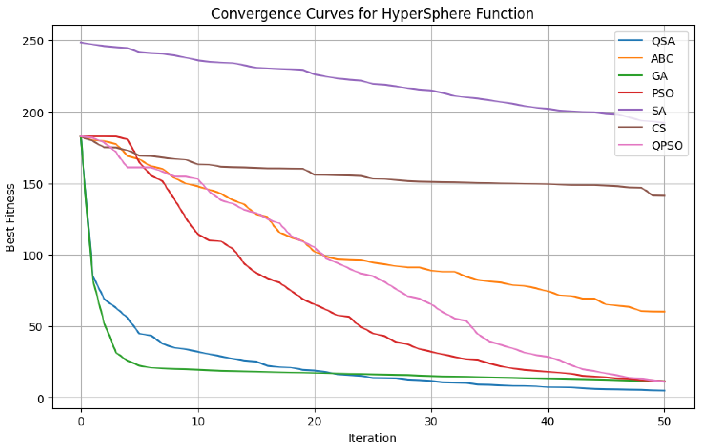
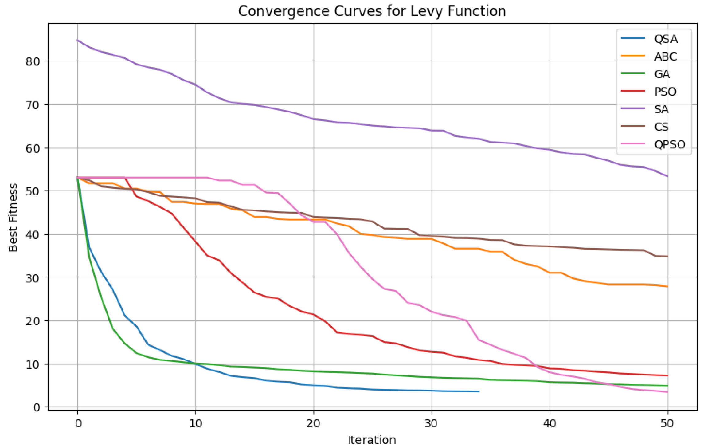
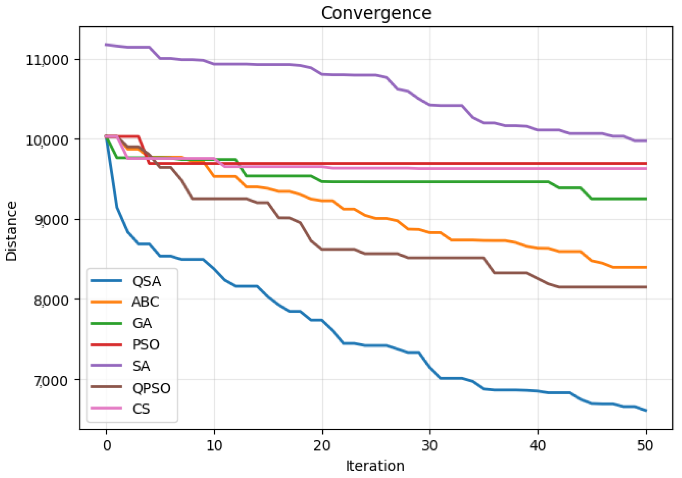
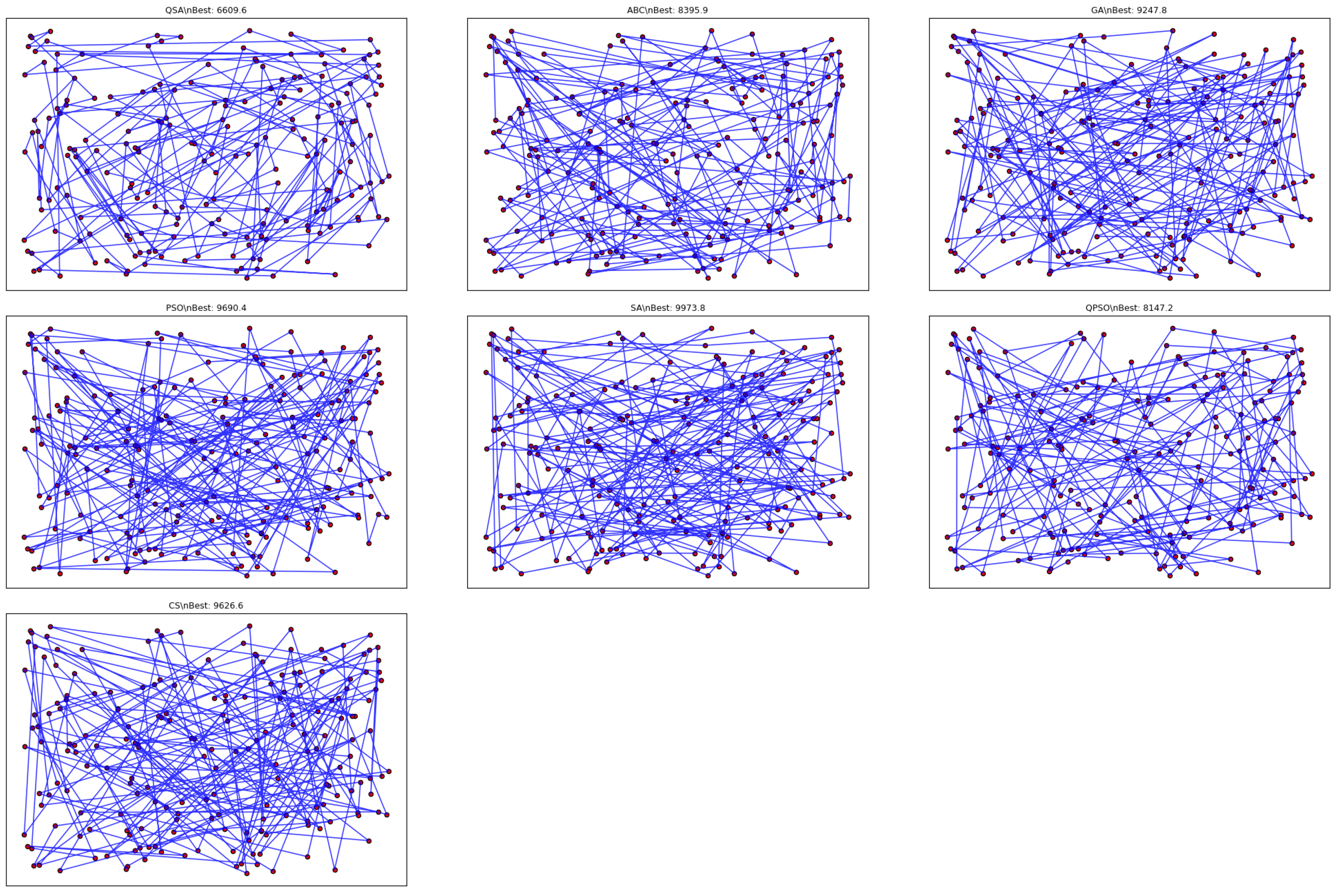
We used TSP with 200 cities across QSA, ABC, GA, SA, PSO, CS, and QPSO in our analysis. The QSA has fared better than other algorithms in the experiment. Additionally, QSA has outperformed the Lévy and HyperSphere test functions.
In order to extend the algorithm’s use beyond the well-known TSP into a variety of distinct domains, including job-shop scheduling, subset selection in feature engineering, and graph-based network design problems, this comprehensive design aims to achieve a well-rounded exploration–exploitation balance. This holistic design of QSA seeks to increase search efficiency, balance exploration and exploitation, and provide greater flexibility for combinatorial and high-dimensional optimization tasks by combining these methods.

2. Materials and Methods

The QSA mathematical model incorporates two unique natural observations:
Snowflake Non-Collision: Snowflakes appear to move randomly as they fall from the sky, but they hardly ever intersect. The collision term in the QSA, which repels agents from one another in the continuous auxiliary space, is based on this observation.
Unique Snowflake Structure: Each snowflake forms a unique crystalline pattern. The QSA maintains agent diversity by employing collisions and quantum leaps to preserve discrete solutions, distinct positions, and the avoidance of solutions rapidly convergent into a single configuration. Equations (8) and (9) partially model this uniqueness characteristic by using quantum leaps and repulsion to maintain distinct solutions. Thus, the “snowflake” analogy is reflected in the algorithm’s name and embedded in its collision avoidance and diversity maintenance mechanics.

2.1. Structure of QSA

2.1.1. General Discrete Optimization Setting

We let X be a discrete solution space (e.g., all permutations of n elements, or all binary vectors of length n, etc.). F : X R be our cost (or objective) function we want to minimize
min x X F ( x ) .
A typical example is that each x X encodes a candidate solution (such as a route in the TSP, a schedule in scheduling problems, or a binary vector for subset selection). The function F ( x ) evaluates how “good” or “bad” that solution is (lower is better). X might be extremely large (e.g., | X | = n ! for permutations).
The QSA addresses this difficulty by maintaining multiple solutions (a population) and employing quantum-inspired moves to jump out of local minima.

2.1.2. Population and Positions

Population: We store P solutions { x ( 1 ) , x ( 2 ) , , x ( P ) } X . Each solution x ( k ) is an element of the discrete search space.
Continuous Positions: We associate each discrete solution x ( k ) with a vector pos ( k ) R d . The dimension d can be chosen based on the problem. If the dimension is large (e.g., d = n ), one can store partial “coordinates” for each variable. If the dimension is small (e.g., d = 2 or d = 3 ), pos ( k ) might represent a more compressed or aggregated feature of x ( k ) .
The mapping Inspiration: Snowflakes all form distinct crystals, each occupying a unique “position” in the sky while descending. In QSA, the mapping Embed : X R d is problem-specific. For instance, in the TSP one might use the centroid of the cities in a given route. In a binary vector problem, pos ( k ) might store real-coded approximations of the binary values. These positions are updated via thermal, collision, and tunneling effects. We then map them back to discrete solutions. The synergy between continuous moves and discrete acceptance is the key to QSA’s “quantum snowflake” style.

2.1.3. Objective Function and Best Solution Tracking

We define
F min = min 1 k P F x ( k ) , and x ( best ) = arg min x ( k ) F x ( k ) .
We keep track of the best solution x ( best ) found so far. Its associated best value is F min . Optionally, we might keep pos ( best ) , the continuous position connected to x ( best ) . This “global best” solution helps guide the entire population by providing a reference for quantum tunneling and superposition. The QSA iteration frequently updates F min whenever a solution surpasses (i.e., yields lower cost than) the current best known.

2.1.4. Temperature and Tunneling Schedules

QSA introduces two time-varying parameters to mimic quantum and thermal phenomena.

2.1.5. Temperature T ( t )

T ( t ) = T max α thermal t .
where t is the iteration index, t = 0 , 1 , , T max . T max is the initial or maximum temperature (a positive real number). α thermal ( 0 , 1 ) is the cooling rate. This temperature value scales the amplitude of random “thermal” displacements.

2.1.6. Tunneling Width σ ( t )

σ ( t ) = σ init α σ t .
where σ init > 0 is the initial tunneling range. α σ ( 0 , 1 ) is another decay factor controlling how quickly tunneling shrinks. These two schedules allow QSA to start more explorative (with higher random movement) and gradually reduce noise, focusing on exploitation in later stages. T ( t ) is analogous to the temperature in simulated annealing, controlling the scale of random kicks. σ ( t ) influences how strongly an agent can “tunnel” toward the best solution, especially if pos ( k ) is far from pos ( best ) .

2.1.7. Thermal Fluctuations

For each agent k, we add a Gaussian random vector (in R d ) scaled by T ( t ) :
thermal ( k ) = T ( t ) ε , ε N 0 , I d × d .
That is, each coordinate of ε is an independent standard normal random variable. The multiplication by T ( t ) ensures that the overall magnitude of these “thermal” moves typically decreases over time. At early iterations, large random steps help explore the solution space. As t increases and T ( t ) drops, these random steps become smaller, refining solutions around local minima.

2.1.8. Quantum Tunneling

We define a “tunneling term” to help solutions “jump over” high-cost barriers:
tunnel ( k ) = β tunnel exp pos ( k ) pos ( best ) 2 σ ( t ) ε ˜ .
where β tunnel is a constant that scales the maximum tunneling strength. ε ˜ N ( 0 , I d × d ) .
The exponential factor
exp pos ( k ) pos ( best ) 2 σ ( t )
ensures that if pos ( k ) is quite distant from pos ( best ) , the agent receives a stronger “push,” facilitating a chance to leap closer. As σ ( t ) decreases over iterations, the tunneling region narrows, focusing more precisely around the best solution. This is metaphorically quantum because it simulates “tunneling through” an energy barrier in physics. If pos ( k ) pos ( best ) is large, the exponential might be significant for early t; but as t grows, σ ( t ) shrinks, limiting these quantum leaps in later stages.

2.1.9. Collision Forces

We assume a neighbor structure among the agents in the continuous space. Suppose agent k has neighbors N k . For each neighbor m N k , we define a displacement
d k , m = pos ( k ) pos ( m ) , d k , m = d k , m , d k , m .
Then, the collision vector for agent k is computed as
collision ( k ) = γ m N k d k , m d k , m + ϵ .
Here, γ is a collision factor (typically around 1.0–2.0) and ϵ 10 9 is a small constant to avoid division by zero. This sum repels each agent from its neighbors, preventing them from clustering too tightly. Collision fosters diversity in the population. If multiple agents converge to the same region, the collision term pushes them away from each other. Overly large γ can scatter solutions too far, while overly small γ may not maintain sufficient diversity. Tuning is problem-dependent.

2.1.10. Position Update Formula

Putting all these components together, for each agent k at iteration t, the new position is
pos new ( k ) = pos ( k ) + thermal ( k ) + δ pos ( best ) pos ( k ) collision ( k ) + tunnel ( k ) .
where thermal ( k ) is the random (Gaussian) step scaled by T ( t ) . δ ( 0 , 1 ) is the pull-to-best coefficient. For instance, if δ 0.8 , the agent strongly gravitates toward the best solution’s position. collision ( k ) is the sum of repulsion from neighbors. tunnel ( k ) is the quantum leap, dependent on σ ( t ) .
Signs: the collision term is subtracted ( collision ( k ) ) to push the agent away from congested areas. The term δ ( pos ( best ) pos ( k ) ) ensures a convergence pressure, while thermal and tunneling promote exploration. Typically, not every iteration includes collision or tunneling; some variants perform collision every few iterations or gradually reduce β tunnel .

2.1.11. Discrete Re-Mapping

After calculating the new position pos new ( k ) , we convert it back into a discrete solution. We denote this mapping as
x candidate ( k ) = g pos new ( k ) X .
This function g is problem-dependent. For example, if X are permutations, one might interpret each coordinate of pos new ( k ) as a priority or rank, then sort them to obtain a permutation. If X are binary vectors, each coordinate may be thresholded to 0/1. If X is a subset of a Euclidean space, the nearest discrete points may be selected. As a comment, the choice of g heavily influences the algorithm’s performance. This step is crucial because the rest of the QSA steps (thermal, collision, tunneling) occur in a continuous auxiliary space, yet the final objective F is always computed on a discrete x ( k ) .

2.1.12. Superposition of Solutions

To accelerate the diffusion of good partial solutions, QSA uses a superposition step. We let p super ( 0 , 1 ) be the probability that an agent attempts superposition with the current best solution. Then, with probability p super , we pick a substructure S x ( best ) . (For example, in permutations, we select a subsegment; in binary vectors, we choose a contiguous or random subset of bits.) We remove from x candidate ( k ) any elements that appear in S. We reinsert S into x candidate ( k ) at a random position or in a consistent manner.
Formally, one might denote
x candidate ( k ) Superpose x candidate ( k ) , x ( best ) , segment or subset S .
This step fosters the spread of high-quality building blocks from the best solution throughout the entire population. If used frequently, superposition can cause premature convergence (i.e., all agents copying the best substructure). If used sparingly, it helps solutions gradually incorporate strong partial solutions while maintaining diversity.

2.1.13. Local Search

After superposition, each solution x candidate ( k ) may undergo a local search operator L . We define
x improved ( k ) = L x candidate ( k ) .
Examples include the follwoing. 2-Opt for permutations: we systematically (or randomly) check whether swapping edges or reversing sub-routes yields a lower cost. 1-bit or k-bit flips for binary vectors: we test whether flipping bits improves the cost. Gradient-based or other metaheuristic operators are used in specialized domains. Local search can be time-consuming; therefore, it is typically limited (e.g., a fixed number of random 2-Opt trials). This ensures that the algorithm does not rely solely on random moves in the continuous space—the local search provides a final “fine-tuning” in the discrete space.

2.1.14. Acceptance Criterion (Greedy or Otherwise)

A common QSA approach is a greedy acceptance rule:
if F x improved ( k ) < F x ( k ) x ( k ) x improved ( k ) .
otherwise, the old x ( k ) is retained. This ensures that the overall best cost in the population does not degrade. Alternative acceptance rules (e.g., with a small probability of accepting a worse solution) are possible. This is simpler than classical simulated annealing, which might accept worse solutions. Since the quantum aspects (tunneling, collision) already maintain exploration, a purely greedy acceptance is often sufficient.

2.1.15. Update Global Best and Early Stopping

After all agents are updated, we first find the best cost in the updated population:
F min , new = min 1 k P F x ( k ) .
If F min , new < F min , then set
F min F min , new , x ( best ) arg min x ( k ) F ( x ( k ) ) .
Early stopping: If F min does not improve for maxNoImprove consecutive iterations, we terminate the loop early. This step ensures the global best solution is always tracked. Early stopping is practical: once the population converges or no further improvement is likely, the algorithm stops to save computation. The step-by-step procedure of the proposed QSA is detailed in algorithm in Section 2.1.16.

2.1.16. Complete Iteration Pseudocode

Bringing all the steps together, we present the following verbose pseudocode:
  • Initialization:
    for  k = 1 P :
    1.1 x ( k ) RandomSolution ( )
    1.2 pos ( k ) Embed x ( k )
    1.3 Evaluate F x ( k )
    end
    Let F min = min 1 k P F x ( k ) .
    Let x ( best ) = arg min x ( k ) F ( x ( k ) ) .
    pos ( best ) Embed ( x ( best ) ) .
    Initialize noImproveCount = 0 .
  • For  t = 0 T max :
    2.1 (Optional) Build a neighbor structure for collision (e.g., using cKDTree or a distance-based method to find N k ).
    2.2 Thermal and Tunneling: For each k,
    thermal ( k ) = T ( t ) ε ,
    tunnel ( k ) = β tunnel exp pos ( k ) pos ( best ) 2 σ ( t ) ε ˜ .
    2.3 Collision: For each k,
    collision ( k ) = γ m N k pos ( k ) pos ( m ) pos ( k ) pos ( m ) + ϵ .
    2.4 Update positions:
    pos ( k ) pos ( k ) + thermal ( k ) + δ pos ( best ) pos ( k ) collision ( k ) + tunnel ( k ) .
    2.5 Discrete Mapping:
    x candidate ( k ) = g pos ( k ) .
    2.6 Superposition (with probability p super ):
    x candidate ( k ) Superpose x candidate ( k ) , x ( best ) .
    2.7 Local Search:
    x improved ( k ) = L x candidate ( k ) .
    2.8 Greedy Acceptance:
    if F ( x improved ( k ) ) < F ( x ( k ) ) x ( k ) x improved ( k ) .
        end for all k.
    2.9 Update  x ( best ) . If any x ( k ) improved the global best, record it.
    2.10 If F min did not change, increment noImproveCount, else reset noImproveCount = 0 .
    2.11 Early Stopping: If noImproveCount maxNoImprove , break.
  • End: Return x ( best ) as the final solution.
Code Availability: The complete source code for the proposed QSA algorithm—implemented in Python (v 3.13.3) and MATLAB (R2024b)—is publicly hosted on GitHub and has been accessible since 1 March 2025: https://github.com/OQSA/OQSA.

2.1.17. Tuning and Practical Considerations

  • Choice of d: The dimension for pos ( k ) can range from very small ( d = 2 ) to quite large ( d n ). Lower d is simpler but may cause less flexible mappings.
  • Collision Frequency: Some QSA implementations perform collision computations only every few iterations to reduce overhead.
  • Tunneling Attenuation:  α σ is often around 0.9, meaning σ ( t ) decays gradually. If it decays too quickly, the quantum leaps may be lost prematurely.
  • Local Search Intensity:  L can be a mild random improvement or an extensive search. More intense local search might slow each iteration but yield better solutions faster.
  • Superposition Probability:  p super is typically set between 0.05 and 0.3. If set too high, the population might converge too quickly; if too low, good building blocks may spread too slowly.

2.2. Core Insights of QSA

  • Hybrid: QSA merges quantum-like “tunneling” and classical “thermal” updates with local search and partial structure mixing (superposition).
  • Exploration–Exploitation Balance: Thermal and tunneling encourage exploration, especially in early iterations. Pull-to-best and local search intensify exploitation in later iterations.
  • Population Diversity: Maintained by collision forces. Without collision, the population might cluster too quickly around a single solution.
  • Adaptability: By modifying the discrete mapping g, superposition rules, and local search, QSA can be adapted to various combinatorial problems.
The QSA can be viewed as a meta-heuristic framework that embeds discrete solutions in a continuous space R d ; simulates “thermal” motions and “quantum” leaps to escape local minima; employs collision for diversity and superposition for knowledge sharing; uses local search to refine solutions and a greedy acceptance scheme to ensure progress.
This structure allows QSA to handle large-scale or complex discrete optimization problems by systematically combining random exploration with best-solution guidance and local neighborhood improvements. Each formula described above contributes to one of the key pillars of the approach, ensuring a deep balance between exploration (via random or quantum moves) and exploitation (through local search and best-solution guidance) throughout the iterative process.

2.3. Application of Test Functions

In this study, we conduct a benchmarking analysis of multiple population-based metaheuristic algorithms. The algorithms under scrutiny include the QSA, ABC, GA, PSO, SA, CS, and OPSO. The evaluation is conducted using two well-known continuous test functions: the HyperSphere (Sphere) function and the Lévy function. These test functions are commonly used to evaluate the performance of optimization algorithms in both unimodal and multimodal search spaces. The process of benchmarking is conducted through the utilisation of Python programming. The Python and Matlab code for QSA and other algorithms can be downloaded from the GitHub repository at https://github.com/OQSA/OQSA.

Definitions of Test Functions

We applied the HyperSphere and the Lévy function for becnhmarking. The HyperSphere function is representative of a unimodal and convex optimization problem. It provides a simple test for the convergence speed and numerical accuracy of optimization algorithms in a smooth landscape. In contrast, the Lévy function exhibits a complex, multimodal search space with many local optima. It is used to evaluate an algorithm’s exploration capabilities and its robustness in avoiding premature convergence to local minima.
HyperSphere (Sphere) Function: The HyperSphere function, also known as the Sphere function, is a fundamental test function used in optimization. It is mathematically defined as follows:
f Sphere ( x ) = i = 1 n x i 2 ,
where
x = ( x 1 , x 2 , , x n ) R n .
Global Optimum: The function achieves its global minimum at
f ( 0 ) = 0 , when x = 0 .
This implies that the best possible solution occurs when all variables are set to zero.
Unimodal Nature: The function is unimodal. This property, which is defined shortly, ensures that optimization algorithms do not become trapped in local minima. Instead they reach a single global minimum. For this reason, the function has been proven to be an excellent benchmark for global optimization techniques.
Convex and Smooth Search Space: It has been demonstrated that the function is convex, which guarantees that any local search method eventually converges to the global minimum. Additionally, its smooth gradient makes it highly suitable for gradient-based optimization algorithms.
Scalability: Since the function is defined in an n-dimensional space, it is widely used to benchmark optimization algorithms for different problem sizes. The computational complexity of evaluating the function grows linearly with the number of dimensions, making it a scalable test function.
Applications: The HyperSphere function is widely utilized in optimization research for benchmarking metaheuristic optimization algorithms such as GA, PSO, and Differential Evolution (DE), evaluating the performance of algorithms on continuous, differentiable, and convex landscapes. Analyzing the behavior of optimization methods in simple, gradient-friendly search spaces before applying them to more complex functions.
Conclusion: The HyperSphere function serves as a fundamental benchmark in optimization studies. Its convex and smooth nature makes it an ideal test function for evaluating the performance of different optimization methods before applying them to real-world, complex, and multi-modal problems.
The Lévy Function: The Lévy function is utilized as a benchmark test function in the present comparative study of metaheuristic algorithms. This function is widely recognized for its complex, multi-modal landscape, which poses a significant challenge for global optimization methods. It is defined as follows:
w i = 1 + 4 x i 1 4 , i = 1 , 2 , , n .
The function is then formulated as
f Levy ( x ) = sin 2 ( π w 1 ) + i = 1 n 1 ( w i 1 ) 2 1 + 10 sin 2 ( π w i + 1 ) + ( w n 1 ) 2 1 + sin 2 ( 2 π w n ) .
Properties: The function is characterized as multimodal, indicating the presence of multiple local minima. The global minimum is located at
f Levy ( x * ) = 0 , where x * = ( 1 , 1 , , 1 ) .
It is widely used for testing optimization algorithms due to its complex landscape with many local optima.
Applications: The Lévy function finds application in the following areas: Benchmarking metaheuristic optimization algorithms; Assessing the capacity of algorithms to extricate themselves from local minima; Evaluating the performance of optimization algorithms in high-dimensional, rugged search spaces.
The Lévy function is a challenging function, which makes it an excellent test function for optimization algorithms that require strong exploration capabilities.

2.4. The Application of the Traveling Salesman Problem to Algorithms

The aim of this study is to illustrate and evaluate our proposed QSA against other metaheuristic algorithms (ABC, GA, PSO, SA, CS, QPSO).
To this end, all methods were applied to a 200-city Traveling Salesman Problem (TSP) instance. The TSP is regarded by many experts in the fields of combinatorial optimization and theoretical computer science as a fundamental problem. In its classical formulation, the TSP is stated as follows: given a set of n “cities” and distances between each pair of cities, the objective is to find a Hamiltonian cycle, defined as a closed route that visits each city exactly once, that minimizes the total travel cost. The TSP is conducted through the utilization of Python programming. The Python code for QSA and other algorithms can be downloaded from the GitHub repository at https://github.com/OQSA/OQSA.

2.4.1. Data Generation and Distance Computation

We generated n = 200 cities as random points in the plane, each with coordinates ( x , y ) [ 0 , 100 ] 2 . The Euclidean distance between any two cities i and j was precomputed and stored in a distance matrix:
d i , j = ( x i x j ) 2 + ( y i y j ) 2 , i , j { 1 , , 200 } , i j .
The pre-computation of pairwise city distances allows each candidate TSP route to be encoded as a permutation of city indices; the total tour length is then obtained by summing the successive city-to-city segments.

2.4.2. Discrete Encoding and Population Initialization

It is evident that each algorithm, including QSA, employs permutations of { 0 , 1 , , 199 } to delineate the TSP tours. An initial population of 25 permutations is randomly generated (one permutation per agent). In QSA’s continuous embedding layer, each permutation x ( k ) is mapped to a 2D centroid, defined as the mean position pos ( k ) R 2 of its city coordinates, for collision and tunneling computations. Despite the simplicity of 2D embeddings, they are sufficient to demonstrate QSA’s collision-based repulsion and quantum leaps.

2.4.3. Collision and Tunneling Mechanics

Collision: In the context of the code, the lines stating “Collision + Tunneling are triggered every few iterations” elucidate the repulsion exhibited by agents whose 2D centroids are in close proximity. This phenomenon, evident in the implementation, functions to circumvent the congregation of tours in the discrete space, thus mirroring the “snowflake” analogy that pertains to the avoidance of collisions.
Tunneling: In the event of an agent’s centroid being a considerable distance from that of the optimal agent, it is possible for said agent to make larger leaps towards the optimal centroid, with said leaps being scaled by a temperature T max that undergoes a decay over the course of iterations. Following the update of the 2D positions, each agent is re-mapped to a permutation via “nearest-route” heuristics (see the Python code in the https://github.com/OQSA/OQSA “Create new route after collision” step).

2.4.4. Superposition and Local Search

Superposition: On occasion, a segment of the optimal route is incorporated into a candidate route, thereby promoting the propagation of favourable partial tours without necessitating complete convergence. This process is initiated with a moderate probability (e.g., 20% in exploration mode).
Local Search: In order to refine the discrete tour, QSA implements a random 2-Opt routine on a select few individuals. This approach involves experimenting with small segment reversals within a permutation, which has been shown to lead to substantial improvements in TSP paths in a limited timeframe.

2.4.5. Iterations and Early Stopping

The value of n iterations is set to 50, and the early stopping criterion is activated in the event of no improvement being observed for eight consecutive steps. Each iteration employs a variety of search algorithms, including collision, tunneling, superposition, and selective local search, to update the population members. The optimal route discovered is documented and its distance is monitored over time.
For the sake of reference, it should be noted that the TSP code segment also implements ABC, GA, PSO, SA, CS and QPSO. In contrast to these methods, none of the aforementioned competitors include a collision or quantum “tunnel” component; instead, they rely on their own canonical operators. Appendix A provides step by step calculation of QSA on a Five-City TSP Instance.

3. Results

3.1. Performance Analysis of Test Functions

The Python code implements seven metaheuristic algorithms (QSA, ABC, GA, PSO, SA, CS and QPSO), with each algorithm being executed 10 times using random seeds to ensure independent runs. The final best fitness value from each run is recorded, and relevant statistical data (minimum, maximum, average, and standard deviation) are presented in Table 1 and Table 2 for HyperSpehere and Lévy functions, respectively. Convergence curves (average best fitness versus iteration) are also plotted in Figure 1 and Figure 2 for HyperSpehere and Lévy functions, respectively.
In the context of the HyperSphere function, which is characterized as a unimodal and convex problem, on the 30–dimensional HyperSphere benchmark, the proposed QSA delivers an unequivocal performance lead. QSA’s mean residual error is a mere 5.04, whereas the closest challengers are more than twice as high—GA at 11.34, PSO at 11.35, and the quantum–inspired QPSO at 11.14—while classical meta-heuristics degrade sharply (ABC 60.15, CS 141.53, SA 192.35). Expressed in relative terms, QSA reduces the average error by approximately 55% versus GA/PSO/QPSO, by 92% versus ABC, and by more than 96% versus CS and SA. Crucially, this dominance is consistent across the entire distribution of runs: QSA’s worst outcome (8.88) is virtually equal to GA’s best (7.14) and remains well below every competitor’s mean. Moreover, QSA exhibits the tightest dispersion ( σ = 1.87 ), underscoring its stability. Combined with the highly significant ANOVA ( F = 948.23 ,   p < 10 15 ), these findings confirm that QSA not only attains the lowest error but also delivers the most dependable solutions on this challenging high-dimensional landscape.
The performance of QSA is further highlighted by the Lévy function, which represents a more challenging multimodal landscape. On the 30-dimensional Lévy benchmark, the proposed QSA again proves to be the most reliable performer. Although GA attains a marginally smaller single best value (1.8976) than QSA’s 1.9176, QSA dominates every aggregate metric that matters for practical optimization: its mean error is only 2.90, which is 40% lower than GA (4.87), 60% lower than PSO (7.21), and nearly an order of magnitude lower—about 90%—than ABC (27.83), CS (34.79) and SA (53.29). Even against the quantum-inspired QPSO, QSA trims the average error by ≈15%. QSA’s consistency is equally compelling: it exhibits the tightest dispersion ( σ = 0.72 ), and its worst-case run (3.96) still lies far below the means of all competing solvers, underscoring a narrow, dependable convergence profile.
Statistical analysis corroborates these observations. A one-way ANOVA across the seven algorithms yields F = 704.59 with p < 1 × 10 15 , confirming that their mean errors differ significantly. Taken together with the pair-wise test results reported earlier, these figures demonstrate that QSA not only approaches the global optimum but does so with a stability and repeatability unmatched by any of the six reference algorithms on this rugged search landscape.
The findings demonstrate that QSA surpasses competing algorithms in both unimodal (HyperSphere) and multimodal (Lévy) test scenarios. The superior performance of QSA can be attributed to its hybrid search strategy, which integrates local exploitation (via elite individual perturbations and superposition moves) with global exploration (through collision and tunnelling mechanisms). The early stopping criterion implemented in QSA, which terminates the iterative process when no improvement is observed for 20% of the maximum iterations (i.e., 10 out of 50 iterations), prevents unnecessary computational effort once convergence is reached. This enhances computational efficiency and contributes to the consistent quality of the solutions obtained by QSA. In summary, the empirical evidence substantiates the conclusion that QSA is a highly effective and robust algorithm for continuous optimization problems. Its capacity to attain lower average fitness values with reduced variability across independent runs signifies its superiority over traditional algorithms such as ABC, GA, PSO, SA, CS, and QPSO when applied to both simple convex functions and more complex multimodal landscapes.

3.2. Performance Analysis of The Traveling Salesman Problem

Table 3 presents a concise overview of the experimental findings, wherein QSA is juxtaposed with four alternative metaheuristics (namely ABC, GA, PSO, SA, CS, and QPSO) in the context of a 200-city TSP. Each algorithm was permitted to execute until either convergence was attained or a predefined iteration limit was reached. The optimal route distance and its corresponding wall-clock time are documented.
As shown in Table 3, QSA delivered the most compact tour while maintaining competitive execution time. QSA attained a best-of-run distance of 6609.61, outperforming every comparator by a wide margin: its tour is 21.3% shorter than ABC (8395.93), 28.5% shorter than GA (9247.81), 31.8% shorter than PSO (9690.38), 33.7% shorter than SA (9973.85), 18.9% shorter than the quantum-inspired QPSO (8147.23), and 31.3% shorter than CS (9626.59). From a computational effort perspective, QSA required only 0.84 s to reach its best solution, placing it firmly in the sub-second regime shared by most heuristic baselines and rendering it nearly an order of magnitude faster than PSO (6.68 s). Although ABC, SA, and QPSO terminated slightly sooner (0.36 s, 0.20 s, and 0.26 s, respectively), the dramatic reduction in tour length achieved by QSA more than compensates for this modest time overhead. In practical terms, QSA offers the best distance–time trade-off: it is the only solver that combines sub-second convergence with a tour length at least one-fifth shorter than any competitor. These findings reinforce our continuous-domain results and underscore QSA’s versatility as a high-quality, time-efficient meta-heuristic for large-scale discrete optimisation.
Figure 3 shows convergence curves for different optimization algorithms on the TSP function that represents the iteration number, while the best fitness value achieved at each step.
Figure 4 provides a visual representation of the “best route” solution obtained by each algorithm (QSA, ABC, GA, PSO, SA, QPSO, and CS) for the 200-city TSP instance. While initially, each of the resulting tours appears visually dense with numerous intersecting edges, two key observations can be made. Upon comparison of the plots, it is evident that subtle variations in edge lengths and angles collectively exert a significant influence on the total route distance. Modifications in the sequence of visited cities can result in a reduction in excessively elongated segments that extend across the entirety of the 100x100 area. Notably, QSA’s solution, despite its intricate nature, attains the lowest overall distance through the minimization of extended “detours” and the balancing of local city clusters. Moreover, visually, all tours appear to be equally “tangled” due to the necessity of connecting 200 points without overlaps in visitation. However, an algorithm that achieves a shorter total distance is likely to have fewer extremely long edges that span diagonally across the region. For instance, a concentration of smaller segments or more orderly sub-loops suggests the algorithm’s capacity to exploit local proximity effectively.

4. Discussion

QSA is introduced as a new algorithm to the literature by combining collision-based diversity preservation, quantum-inspired tunneling, overlap-based partial solution sharing, and local optimization to address a wide range of continuous and discrete optimization problems. QSA is evaluated on multiple test functions, such as Lévy and HyperSphere in the continuous domain, and on a large-scale TSP in the discrete domain. As indicated in Table 4, Toaza and Esztergár-Kiss [23] conducted a detailed review of metaheuristic approaches for TSP-based scheduling optimization challenges. We compared ABC, GA, PSO, SA, CS, and QPSO with our novel algorithm QSA. So, we used these metahuristics to compare our method.
We compared the most widely used baseline optimization algorithms in the literature, ABC, GA, PSO, SA, CS, and QPSO, with our new algorithm. QSA in our testing was shown to consistently obtain low function values (around the global minimum) in fewer iterations. In experiments, QSA reached the best value with an average fitness value of 5.0449 on the HyperSphere benchmark, showing robust exploitation with enough exploration. Moreover, QSA’s quantum tunnelling enabled it to avoid local troughs more efficiently than the other algorithms which are swarm or evolutionary algorithms on the Lévy benchmark. Lévy is a deceptively multimodal terrain. QSA outperformed the others with an average fitness value of 2.9017 on the Lévy benchmark. In QSA, the incorporation of solutions within a continuous auxiliary space, in conjunction with the implementation of repulsive forces, was demonstrated to effectively mitigate the occurrence of premature clustering, a prevalent limitation of other algorithms such as GA and PSO. The collision-based dynamics of the algorithm were shown to impede the convergence of the search process on local minima, thereby fostering the exploration of more extensive search spaces and enhancing the efficacy of the global search process. Moreover, early iterations leveraged higher thermal energy to sample the space widely, while decaying σ values gradually reinforced tunneling around high-value basins. These elements worked together to offer QSA consistently low function values and rapid convergence. The TSP performance showed that QSA required a considerable amount of wall-clock time, but it produced the shortest route distance with a value of 6567.58 in our experiment. The mapping of permutations into a continuous 2D space allowed the collision and tunneling stages to function consistently. Following position updates, solutions were remapped to permutations via nearest-route or partial reinsertions, thereby allowing QSA to combine “snowflake” diversity and quantum leaps effectively in a purely combinatorial context. The superposition stage of QSA inserts quality sub-segments from the best solution into others, thereby accelerating the spread of partial “good routes”. The subsequent 2-Opt–based local search further pruned unnecessary detours. It is evident that, collectively, these operators enhanced the algorithm’s exploitation capacity, whilst collisions ensured that variety was maintained in possible tours.
Overall, the multi-faceted design of QSA—merging collision-based swarm behavior, quantum leaps, partial superposition, and local search—proved advantageous. Whether tackling continuous or discrete domains, the algorithm maintained a strong balance of exploration (through collisions and tunneling) and exploitation (through local search and best-solution-based superposition).
Our experimental analysis on the 30-dimensional Lévy benchmark demonstrates the clear statistical superiority of the proposed QSA. A one-way ANOVA applied to the seven competing meta-heuristics produced an F - value = 704.59 with p < 1 × 10 15 , unequivocally confirming overall performance differences. Follow-up pair-wise t-tests ( α = 0.05 , unadjusted) further revealed that QSA delivers a significantly lower average error than every rival: ABC  ( t = 22.79 , p < 1 × 10 15 ) , GA  ( t = 5.54 , p = 7.8 × 10 7 ) , PSO  ( t = 9.34 , p = 3.6 × 10 13 ) , SA  ( t = 43.87 , p < 1 × 10 15 ) , CS  ( t = 31.04 ,   p < 1 × 10 15 ), and even the quantum-inspired QPSO  ( t = 2.10 , p = 0.040 ) . Collectively, these statistics substantiate QSA’s dominance in high-dimensional continuous optimisation and underscore its promise as a robust, state-of-the-art solver for complex search spaces.
On the 30-dimensional HyperSphere benchmark, the proposed QSA once more demonstrated decisive superiority. A one-way ANOVA conducted across the seven competing meta-heuristics produced an F = 948.23 with p 1 × 10 16 , leaving no doubt that the algorithms’ mean errors differ substantially. Subsequent pair-wise two-sample t-tests ( α = 0.05 , unadjusted) confirmed that QSA outperforms every rival by a comfortable statistical margin: ABC  ( t = 29.88 , p < 10 15 ) , GA  ( t = 10.05 , p 2.6 × 10 14 ) , PSO  ( t = 3.57 , p 7.3 × 10 4 ) , SA  ( t = 36.25 , p < 10 15 ) , CS  ( t = 46.83 , p < 10 15 ) , and even the quantum-inspired QPSO  ( t = 7.55 , p 3.5 × 10 10 ) . Collectively, these statistics underscore QSA’s ability to deliver the lowest average error—often by more than an order of magnitude—thereby cementing its status as a robust, state-of-the-art solver for challenging high-dimensional optimisation landscapes.
In metaheuristic optimization algorithms, two factors largely determine whether an algorithm will transition from a promising prototype to a deployable tool: parameter sensitivity and computational complexity. Parameter sensitivity describes how sharply performance responds to small changes in key hyper-parameters—such as population size, exploration–exploitation coefficients, or cooling schedules—which, if not robustly tuned, can lead to erratic convergence or premature stagnation across different problem instances. Computational complexity, encompassing both time and memory requirements, sets the practical ceiling for real-world adoption: an algorithm that delivers marginally better optima yet scales super-linearly in runtime or memory may be infeasible for high-dimensional or real-time applications. Discussing these dimensions in tandem enables fair benchmarking, highlights the trade-offs between accuracy and resource consumption, and guides practitioners in selecting parameter settings that balance solution quality with operational constraints.

5. Conclusions

In this study, the QSA is presented as a flexible metaheuristic framework that has been proven effective for both continuous and discrete optimization. The following are the research’s main conclusions. Sturdy Performance in All Domains: The shortest TSP route was produced among the algorithms examined in this study, and the QSA was shown to perform better or almost as well on Lévy and HyperSphere in the continuous world. One of the study’s highlights is its cross-domain efficacy, which demonstrates how flexible the algorithm is. Collision and Tunneling Synergy: Motivated by snowflakes’ ability to avoid collisions and preserve their unique crystalline forms, QSA uses collision repulsion to maintain population variety and prevent swarm collapse. At the same time, quantum tunneling helps to overcome complex basins and avoid local minima. Superposition and Local Refinement: QSA systematically uses partial solutions from global bests while improving them via random 2-Opt, a small-scale local search. This layered approach provides a powerful combination of intensification and controlled cross-solution mixing. Discrete–Continuous Interplay: By embedding discrete solutions (e.g., permutations for TSP) into a continuous vector space, QSA applies uniform collision, tunnelling, and thermal updates. The method is not restricted to a single domain representation since re-mapping from continuous back to discrete is employed.
We also offer a perspective for future studies. Multi-objective Extensions: QSA can be adapted to multi-criterion problems (e.g., TSP with constraints or hyper-volume objectives) by preserving diverse Pareto solutions through collision. Adaptive Parameter Control: Dynamic adjustments of tunneling density σ ( t ) , collision factors, or overlap ratios increase the convergence reliability and also reduce trial-and-error tuning. Domain-Specific Hybridization: The integration of advanced local heuristics or specialized repair functions (for constrained scheduling or routing) has the potential to further enhance the performance and robustness of the QSA. Scalability Studies: Experiments on higher-dimensional continuous benchmarks and larger discrete problems would help validate QSA’s computational efficiency and near-optimality properties under real-world complexity.
In summary, QSA provides a strong, all-purpose solution mechanism that regularly beats or matches metaheuristics like ABC, GA, PSO, SA, CS, and QPSO in both continuous and discrete benchmarks. Its “snowflake” metaphor—unique individuals that do not collide—combined with quantum-inspired leaps has proven to be more than a conceptual novelty, translating into substantive improvements in solution quality and convergence behavior. As further refinements and adaptive strategies are explored, QSA has the potential to be extended into a versatile tool for a broad spectrum of challenging optimization problems in science and engineering.

Author Contributions

Both Z.O. and B.O. were responsible for algorithm design. Quantum part of algorithm designed by Z.O. The benchmarks were evaulated by B.O. B.O. analyzed the results. All authors have read and approved the final manuscript.

Funding

This research received no external funding.

Institutional Review Board Statement

Not applicable.

Informed Consent Statement

Not applicable.

Data Availability Statement

The complete source code for the proposed QSA algorithm—implemented in Python (v 3.13.3) and MATLAB (R2024b)—is publicly hosted on GitHub and has been accessible since 1 March 2025: https://github.com/OQSA/OQSA.

Conflicts of Interest

The authors declare no conflicts of interest.

Abbreviations

The following abbreviations are used in this manuscript:
ABCArtificial Bee Colony
CSCuckoo Search
DEDifferential Evolution
GAGenetic Algorithm
QAPQuadratic Assignment Problem
QPSOQuantum Particle Swarm Optimization
QSAQuantum Snowflake Algorithm
PSOParticle Swarm Optimization
SASimulated Annealing
TSPTraveling Salesman Problem
VRPVehicle Routing Problem

Appendix A. Step-by-Step Calculation of QSA on a Five-City TSP Instance

To illustrate the mechanics of the proposed Quantum Snowflake Algorithm (QSA) in a fully transparent way, we solve a toy Traveling Salesman Problem (TSP) with n = 5 cities { A , B , C , D , E } . All numerical steps below instantiate the general formulas in Equations (1)–(22).
Table A1. Coordinates of the five cities.
CityABCDE
x00110.5
y01100.5
Table A2. Euclidean distance matrix  d i j .
ABCDE
A01.0001.4141.0000.707
B1.00001.0001.4140.707
C1.4141.00001.0000.707
D1.0001.4141.00000.707
E0.7070.7070.7070.7070

Appendix A.1. Initial Population and Fitness

The best solution after initialization is
x 0 ( best ) = ( A , B , C , D , E ) , F min , 0 = 4.414 .
Table A3. Initial population ( P = 5 ) and tour costs computed with F ( x ) = i = 1 n d x i , x i + 1 .
Agent kRoute x ( k ) (Permutation) F ( x ( k ) )
1 ( A , B , C , D , E ) 4.414
2 ( A , C , B , E , D ) 4.828
3 ( A , D , E , B , C ) 4.828
4 ( A , E , D , C , B ) 4.414
5 ( A , C , E , D , B ) 5.243

Appendix A.2. Embedding to Continuous Space

For demonstration, we embed each permutation to a 2D point pos ( k ) = 1 2 ( x R 1 + x R 2 ) , 1 2 ( y R 1 + y R 2 ) , i.e., the centroid of the first two cities. For Agent 1, ( R 1 , R 2 ) = ( A , B ) pos ( 1 ) = ( 0 , 0.5 ) , and so on.

Appendix A.3. One QSA Iteration (t = 01)

  • Parameter values:
T max = 1.0 , σ init = 0.10 , α thermal = α σ = 0.9 , δ = 0.5 , γ = 1.2 , β tunnel = 1.2 .
  • Agent 1 calculations:
Thermal step (Equation (15)):
thermal ( 1 ) = ( 0.30 , 0.12 ) .
Pull-to-best is zero because Agent 1 is currently the best. Collision vector (Equation (17)) computed from its two nearest neighbors is collision ( 1 ) = ( + 0.14 , 0.09 ) . Quantum tunnelling (Equation (16)) is  0 since pos ( 1 ) = pos ( best ) .
Position update (Equation (18)):
pos new ( 1 ) = ( 0 , 0.5 ) + ( 0.30 , 0.12 ) ( 0.14 , 0.09 ) = ( 0.44 , 0.71 ) .
  • Discrete re-mapping:
Cities are sorted by increasing distance to ( 0.44 , 0.71 ) , yielding the permutation
x candidate ( 1 ) = ( B , A , E , C , D ) .
  • Local search (2-Opt):
Reversing the segment ( A , E ) gives x improved ( 1 ) = ( B , E , A , C , D ) with cost F = 4.000 < 4.414 , hence it is accepted (Equation (22)).
  • Population summary after Iteration 1:
Repeating the above for Agents 2 5 produces new costs { 4.00 , 4.24 , 4.41 , 4.59 } . The global best is updated to
x 1 ( best ) = ( B , E , A , C , D ) , F min , 1 = 4.000 .

Appendix A.4. Convergence

With T ( 1 ) = 0.9 and σ ( 1 ) = 0.09 , the algorithm continues until no improvement is observed for maxNoImprove iterations. For this toy instance, QSA converges within eight iterations to the optimal tour
x = ( A , B , E , C , D ) , F = 3.828 .

References

  1. Rajabioun, R. Cuckoo optimization algorithm. Appl. Soft Comput. 2011, 11, 5508–5518. [Google Scholar] [CrossRef]
  2. Doostmohammadian, M.; Jiang, W.; Liaquat, M.; Aghasi, A.; Zarrabi, H. Discretized distributed optimization over dynamic digraphs. IEEE Trans. Autom. Sci. Eng. 2024, 22, 2758–2767. [Google Scholar] [CrossRef]
  3. Wei, W.; Yang, R.; Gu, H.; Zhao, W.; Chen, C.; Wan, S. Multi-objective optimization for resource allocation in vehicular cloud computing networks. IEEE Trans. Intell. Transp. Syst. 2021, 23, 25536–25545. [Google Scholar] [CrossRef]
  4. Salzman, O.; Halperin, D. Asymptotically near-optimal RRT for fast, high-quality motion planning. IEEE Trans. Robot. 2016, 32, 473–483. [Google Scholar] [CrossRef]
  5. Zhang, Z.; Yang, J. A discrete cuckoo search algorithm for traveling salesman problem and its application in cutting path optimization. Comput. Ind. Eng. 2022, 169, 108157. [Google Scholar] [CrossRef]
  6. Pop, P.C.; Cosma, O.; Sabo, C.; Sitar, C.P. A Comprehensive Survey on the Generalized Traveling Salesman Problem. Eur. J. Oper. Res. 2024, 314, 819–835. [Google Scholar] [CrossRef]
  7. Li, X.; Fang, W.; Zhu, S.; Zhang, X. An Adaptive Binary Quantum-Behaved Particle Swarm Optimization Algorithm for the Multidimensional Knapsack Problem. Swarm Evol. Comput. 2024, 86, 101494. [Google Scholar] [CrossRef]
  8. Dauzère-Pérès, S.; Ding, J.; Shen, L.; Tamssaouet, K. The Flexible Job Shop Scheduling Problem: A Review. Eur. J. Oper. Res. 2024, 314, 409–432. [Google Scholar] [CrossRef]
  9. Fang, J.; Rao, Y.; Luo, Q.; Xu, J. Solving One-Dimensional Cutting Stock Problems with the Deep Reinforcement Learning. Mathematics 2023, 11, 1028. [Google Scholar] [CrossRef]
  10. Li, Z.; Zhou, Y.; Zhang, S.; Song, J. Lévy-Flight Moth-Flame Algorithm for Function Optimization and Engineering Design Problems. Math. Probl. Eng. 2016, 2016, 1423930. [Google Scholar] [CrossRef]
  11. Stoyan, Y.; Yaskov, G.; Romanova, T.; Litvinchev, I.; Yakovlev, S.; Cantú, J.M.V. Optimized Packing Multidimensional Hyperspheres: A Unified Approach. Math. Biosci. Eng. 2020, 17, 6601–6630. [Google Scholar] [CrossRef] [PubMed]
  12. Grigoryev, I.; Mustafina, S. Global Optimization of Functions of Several Variables Using Parallel Technologies. Int. J. Pure Appl. Math. 2016, 106, 301–306. [Google Scholar] [CrossRef]
  13. Johnvictor, A.C.; Durgamahanthi, V.; Pariti Venkata, R.M.; Jethi, N. Critical Review of Bio-Inspired Optimization Techniques. Wiley Interdiscip. Rev. Comput. Stat. 2022, 14, e1528. [Google Scholar] [CrossRef]
  14. Hoffman, K.L.; Padberg, M.; Rinaldi, G. Traveling salesman problem. Encycl. Oper. Res. Manag. Sci. 2013, 1, 1573–1578. [Google Scholar]
  15. Braekers, K.; Ramaekers, K.; Van Nieuwenhuyse, I. The vehicle routing problem: State of the art classification and review. Comput. Ind. Eng. 2016, 99, 300–313. [Google Scholar] [CrossRef]
  16. Pitsoulis, L.; Pardalos, P.M. Quadratic assignment problem. In Encyclopedia of Optimization; Springer: Berlin/Heidelberg, Germany, 2024; pp. 1–35. [Google Scholar]
  17. Liu, Y.; Wang, L.; Wang, X.V.; Xu, X.; Zhang, L. Scheduling in cloud manufacturing: State-of-the-art and research challenges. Int. J. Prod. Res. 2019, 57, 4854–4879. [Google Scholar] [CrossRef]
  18. Knowles, J. ParEGO: A hybrid algorithm with on-line landscape approximation for expensive multiobjective optimization problems. IEEE Trans. Evol. Comput. 2006, 10, 50–66. [Google Scholar] [CrossRef]
  19. Molga, M.; Smutnicki, C. Test functions for optimization needs. Test Funct. Optim. Needs 2005, 101, 32. [Google Scholar]
  20. Johnson, D.S. Experimental analysis of algorithms. In Data Structures, Near Neighbor Searches, and Methodology: Fifth and Sixth DIMACS Implementation Challenges; American Mathematical Society: Providence, RI, USA, 2002; Volume 59, p. 215. [Google Scholar]
  21. Velasco, L.; Guerrero, H.; Hospitaler, A. A literature review and critical analysis of metaheuristics recently developed. Arch. Comput. Methods Eng. 2024, 31, 125–146. [Google Scholar] [CrossRef]
  22. Martí, R.; Sevaux, M.; Sörensen, K. 50 years of metaheuristics. Eur. J. Oper. Res. 2024, 321, 345–362. [Google Scholar] [CrossRef]
  23. Toaza, B.; Esztergár-Kiss, D. A review of metaheuristic algorithms for solving TSP-based scheduling optimization problems. Appl. Soft Comput. 2023, 148, 110908. [Google Scholar] [CrossRef]
  24. Kirkpatrick, S.; Gelatt, C.D., Jr.; Vecchi, M.P. Optimization by simulated annealing. Science 1983, 220, 671–680. [Google Scholar] [CrossRef]
  25. Suman, B.; Kumar, P. A survey of simulated annealing as a tool for single and multiobjective optimization. J. Oper. Res. Soc. 2006, 57, 1143–1160. [Google Scholar] [CrossRef]
  26. Holland, J.H. Genetic algorithms and the optimal allocation of trials. SIAM J. Comput. 1973, 2, 88–105. [Google Scholar] [CrossRef]
  27. Katoch, S.; Chauhan, S.S.; Kumar, V. A review on genetic algorithm: Past, present, and future. Multimed. Tools Appl. 2021, 80, 8091–8126. [Google Scholar] [CrossRef]
  28. Kennedy, J.; Eberhart, R. Particle swarm optimization. In Proceedings of the ICNN’95-International Conference on Neural Networks, Perth, WA, Australia, 27 November–1 December 1995; IEEE: Piscataway, NJ, USA, 1995; Volume 4, pp. 1942–1948. [Google Scholar]
  29. Jain, M.; Saihjpal, V.; Singh, N.; Singh, S.B. An overview of variants and advancements of PSO algorithm. Appl. Sci. 2022, 12, 8392. [Google Scholar] [CrossRef]
  30. Karaboga, D.; Basturk, B. A powerful and efficient algorithm for numerical function optimization: Artificial bee colony (ABC) algorithm. J. Glob. Optim. 2007, 39, 459–471. [Google Scholar] [CrossRef]
  31. Karaboga, D.; Basturk, B. On the performance of artificial bee colony (ABC) algorithm. Appl. Soft Comput. 2008, 8, 687–697. [Google Scholar] [CrossRef]
  32. Pan, Q.K.; Tasgetiren, M.F.; Suganthan, P.N.; Chua, T.J. A discrete artificial bee colony algorithm for the lot-streaming flow shop scheduling problem. Inf. Sci. 2011, 181, 2455–2468. [Google Scholar] [CrossRef]
  33. Ouaarab, A.; Ahiod, B.; Yang, X.S. Discrete Cuckoo Search Algorithm for the Travelling Salesman Problem. Neural Comput. Appl. 2014, 24, 1659–1669. [Google Scholar] [CrossRef]
  34. Hakemi, S.; Houshmand, M.; KheirKhah, E.; Hosseini, S.A. A review of recent advances in quantum-inspired metaheuristics. Evol. Intell. 2024, 17, 627–642. [Google Scholar] [CrossRef] [PubMed]
  35. Fang, W.; Sun, J.; Ding, Y.; Wu, X.; Xu, W. A review of quantum-behaved particle swarm optimization. IETE Tech. Rev. 2010, 27, 336–348. [Google Scholar] [CrossRef]
  36. Blekos, K.; Brand, D.; Ceschini, A.; Chou, C.H.; Li, R.H.; Pandya, K.; Summer, A. A review on quantum approximate optimization algorithm and its variants. Phys. Rep. 2024, 1068, 1–66. [Google Scholar] [CrossRef]
  37. Jiang, J.R.; Shu, Y.C.; Lin, Q.Y. Benchmarks and Recommendations for Quantum, Digital, and GPU Annealers in Combinatorial Optimization. IEEE Access 2024, 12, 125014–125031. [Google Scholar] [CrossRef]
  38. Saad, H.M.H.; Chakrabortty, R.K.; Elsayed, S.; Ryan, M.J. Quantum-inspired genetic algorithm for resource-constrained project-scheduling. IEEE Access 2021, 9, 38488–38502. [Google Scholar] [CrossRef]
  39. Omidvar, M.N.; Li, X.; Yao, X. A review of population-based metaheuristics for large-scale black-box global optimization—Part II. IEEE Trans. Evol. Comput. 2021, 26, 823–843. [Google Scholar] [CrossRef]
  40. Novak, M. The Logic of Legal Argumentation: Multi-Modal Perspectives; Taylor & Francis: Abingdon, UK, 2024. [Google Scholar]
  41. Xie, S.; Yu, Y.; Xie, Y.; Tang, Z. Sensitive Feature Selection for Industrial Flotation Process Soft Sensor based on Multi Swarm PSO with Collaborative Search. IEEE Sens. J. 2024, 24, 17159–17168. [Google Scholar] [CrossRef]
  42. Sadeghi Hesar, A.; Houshmand, M. A memetic quantum-inspired genetic algorithm based on tabu search. Evol. Intell. 2024, 17, 1837–1853. [Google Scholar] [CrossRef]
Figure 1. Convergence curves for the HyperSphere function using different optimization algorithms. The x-axis represents the iteration number, while the y-axis shows the best fitness value achieved at each step.
Applsci 15 05117 g001
Figure 2. Convergence curves for the Lévy function using different optimization algorithms. The x-axis represents the iteration number, while the y-axis shows the best fitness value achieved at each step.
Applsci 15 05117 g002
Figure 3. Convergence curves for different optimization algorithms on the TSP function. The x-axis represents the iteration number, while the y-axis shows the best fitness value achieved at each step.
Applsci 15 05117 g003
Figure 4. Visualization of the TSP routes obtained by different optimization algorithms. Each red dot represents a city, and blue lines indicate the travel paths connecting them. The seven subfigures correspond to different algorithmic approaches applied to the 200-city TSP instance.
Applsci 15 05117 g004
Table 1. Performance comparison of different optimization algorithms on the HyperSphere function (dim = 30, bounds = [−5.12, 5.12]).
AlgorithmBestWorstAverageStd
QSA2.86268.88375.04491.8697
ABC44.124576.628560.14959.9259
GA7.143117.477711.34252.8794
PSO3.404033.988711.35079.5015
SA143.3476237.2534192.349728.2362
CS106.8212159.7109141.525715.8542
QPSO6.199018.843111.14294.0122
Table 2. Performance comparison of different optimization algorithms on the Lévy function (dim = 30, bounds = [−5.12, 5.12]).
AlgorithmBestWorstAverageStd
QSA1.91763.96202.90170.7214
ABC13.184535.590227.82995.9480
GA1.89767.62944.87021.8090
PSO4.197312.75467.20992.4210
SA41.837561.599353.29476.2501
CS23.070741.460134.78975.5807
QPSO1.58335.44243.40591.0968
Table 3. Performance comparison of different optimization algorithms on the 200-city TSP.
AlgorithmBest DistanceElapsed Time (s)
QSA6609.610.84 s
ABC8395.930.36 s
GA9247.810.61 s
PSO9690.386.68 s
SA9973.850.20 s
QPSO8147.230.26 s
CS9626.595.71 s
Table 4. Impact on the TSP (Total Publications) [23].
AlgorithmTotal Publications
Genetic Algorithm2257
Ant Colony Optimization1338
Simulated Annealing775
Particle Swarm Optimization468
Tabu Search330
Memetic Algorithm150
Variable Neighborhood Search143
Artificial Bee Colony98
Differential Evolution96
Firefly Algorithm59
Genetic Programming53
Clonal Selection Algorithm36
Gene Expression Programming33
Disclaimer/Publisher’s Note: The statements, opinions and data contained in all publications are solely those of the individual author(s) and contributor(s) and not of MDPI and/or the editor(s). MDPI and/or the editor(s) disclaim responsibility for any injury to people or property resulting from any ideas, methods, instructions or products referred to in the content.

