
Soft Fuzzy Reinforcement Neural Network Proportional–Derivative Controller


Abstract
1. Introduction
- A model-free SAC framework for fuzzy neural network PD controllers that uses reinforcement learning to automatically adjust fuzzy rules for optimal control.
- Incorporation of expert knowledge: the partial interpretability of FNNs allows expert knowledge to be included during initialization, enabling faster convergence early in training.
- Enhanced training efficiency: the controller uses stochastic optimization and integrates entropy during training, improving exploration efficiency and significantly reducing training time.
- Superior performance: experimental results show that the SFPD controller achieves faster convergence and superior control performance compared to both SAC and traditional PD controllers.
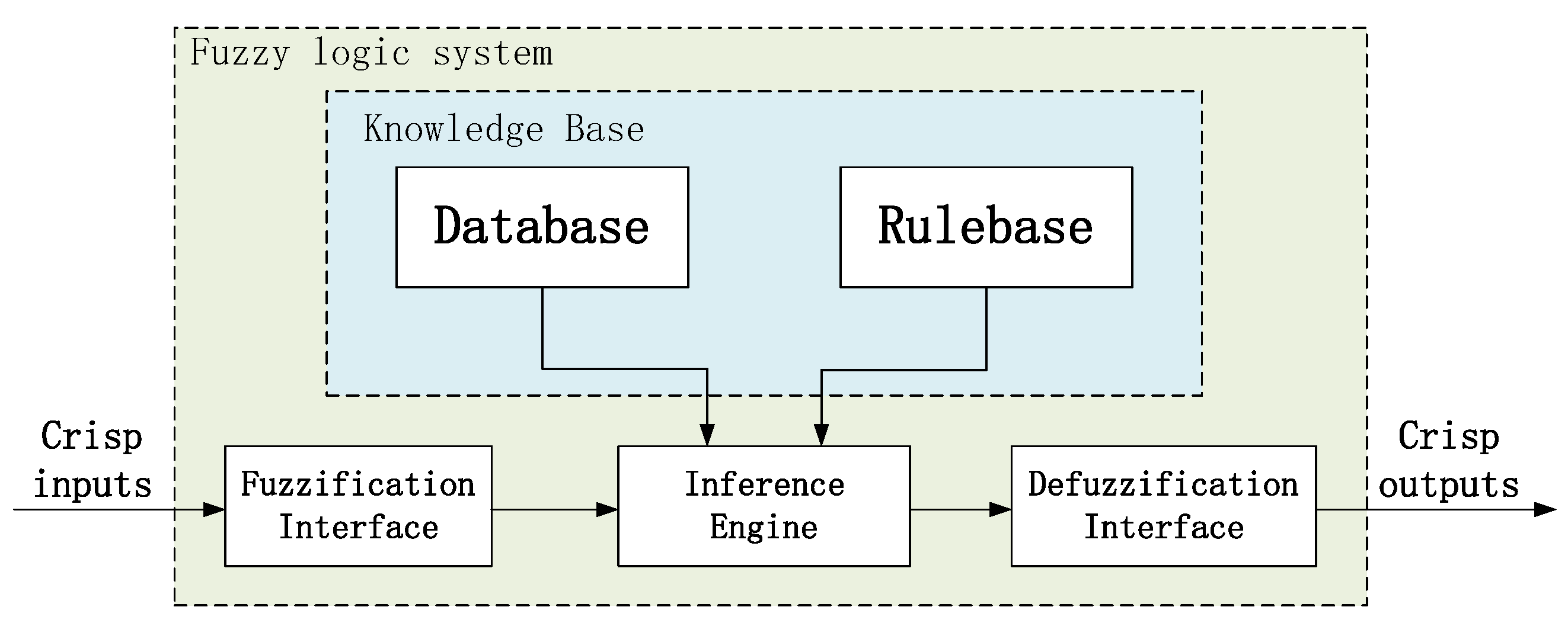
2. Preliminaries
2.1. Reinforcement Learning (RL)
- : the objective function of the policy network.
- : the expected return of a trajectory.
- : a hyperparameter used to balance the weights of return and entropy.
- : the entropy of the policy network distribution.
- : the output of the policy network, which serves as the mean of a Gaussian distribution.
- : the standard deviation of the Gaussian distribution.
- : a sample from the standard normal Gaussian distribution.
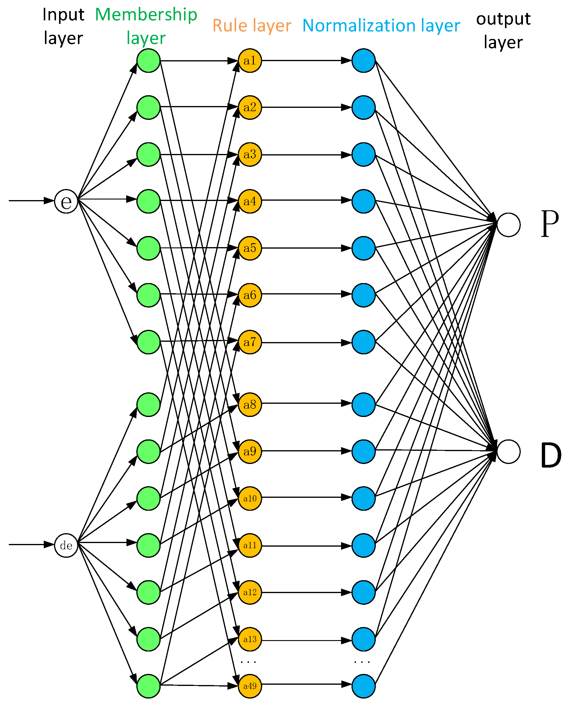
2.2. Fuzzy Neural Network PD (FNNPD) Controller
3. Proposed Soft Fuzzy Reinforcement Neural Network PD (SFPD) Controller
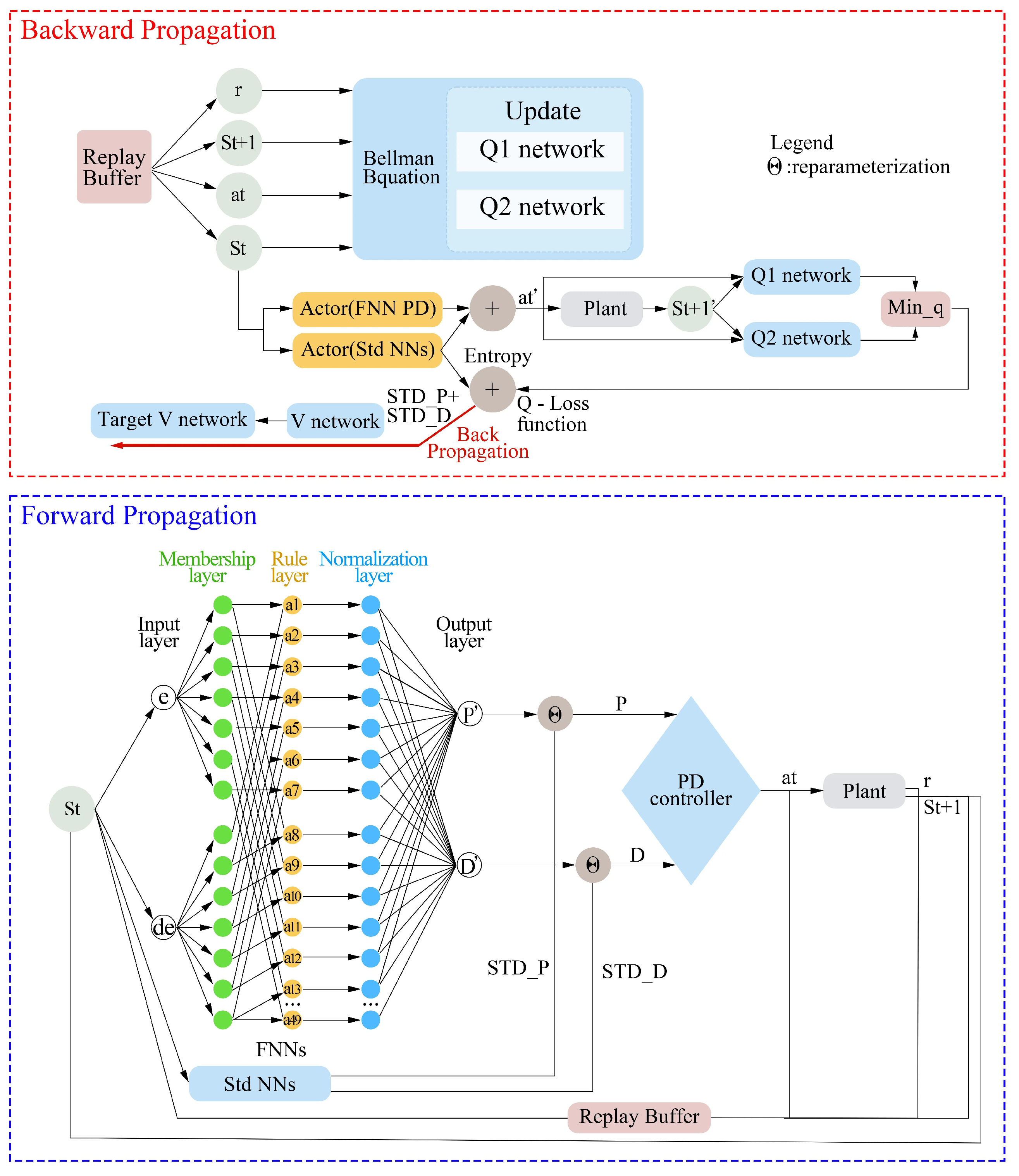
3.1. Forward Propagation
3.2. Backward Propagation
| Algorithm 1 SFPD |
|
4. Results and Discussion
4.1. Experimental Setup
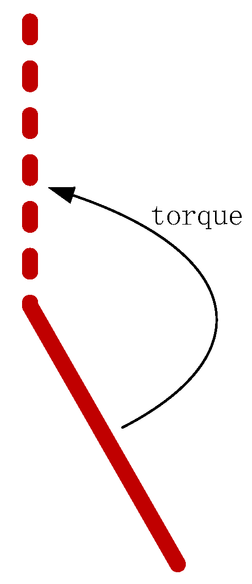
4.1.1. Case 1: Pendulum-v1
System Model
Reward Function
4.1.2. Case 2: CSTR System
System Model
- represents the heat of the reaction per mole;
- denotes the heat capacity coefficient;
- stands for the density coefficient;
- U represents the overall heat transfer coefficient;
- A denotes the area for heat exchange, specifically the interface area between the coolant and vessel.
Reward Function
4.2. Experimental Results
4.2.1. Case 1: Pendulum-v1
Training Performance Evaluation
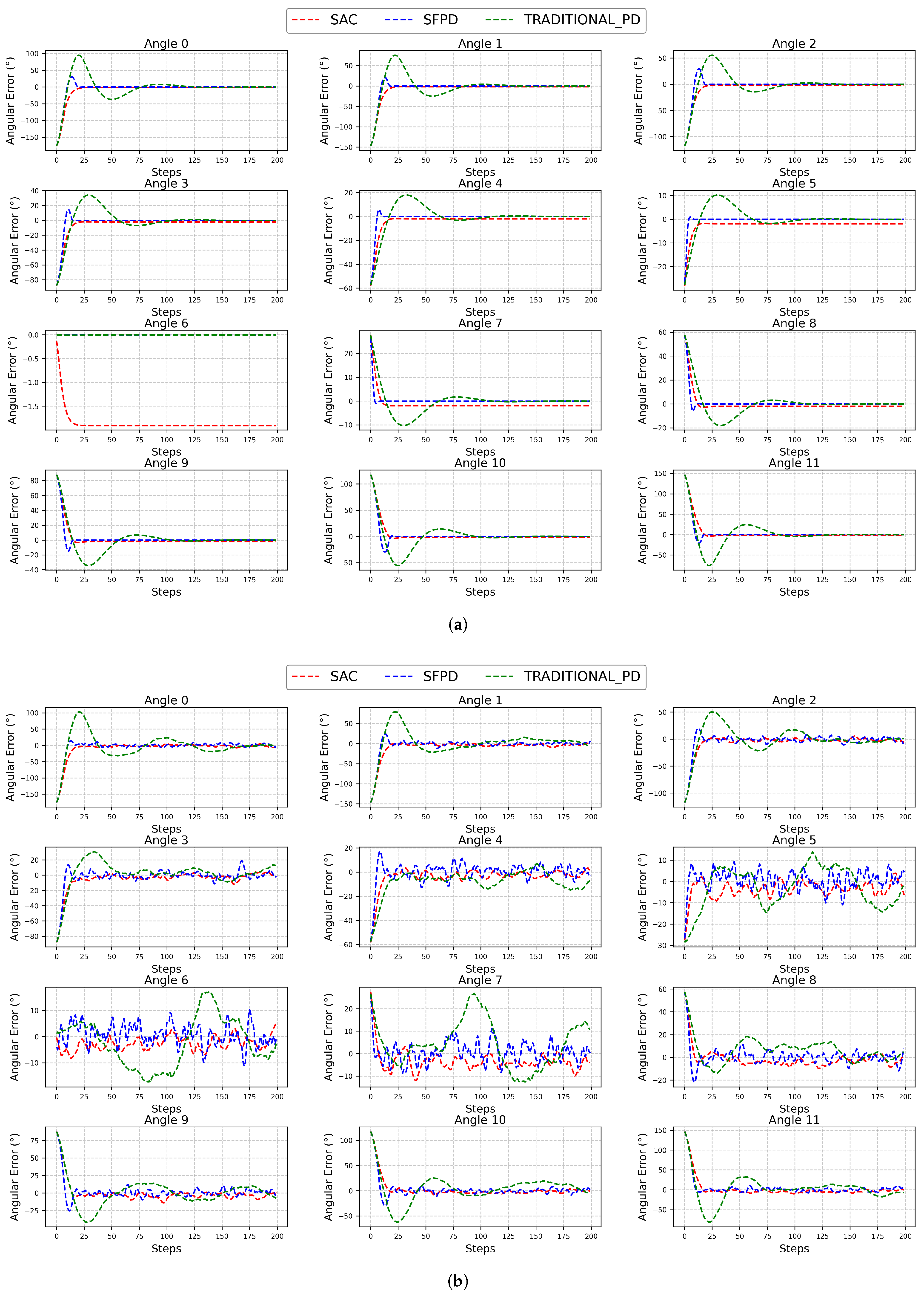
Testing Performance Evaluation
Test with Randomized Initial Conditions
4.2.2. Case 2: CSTR System
Training Performance Evaluation
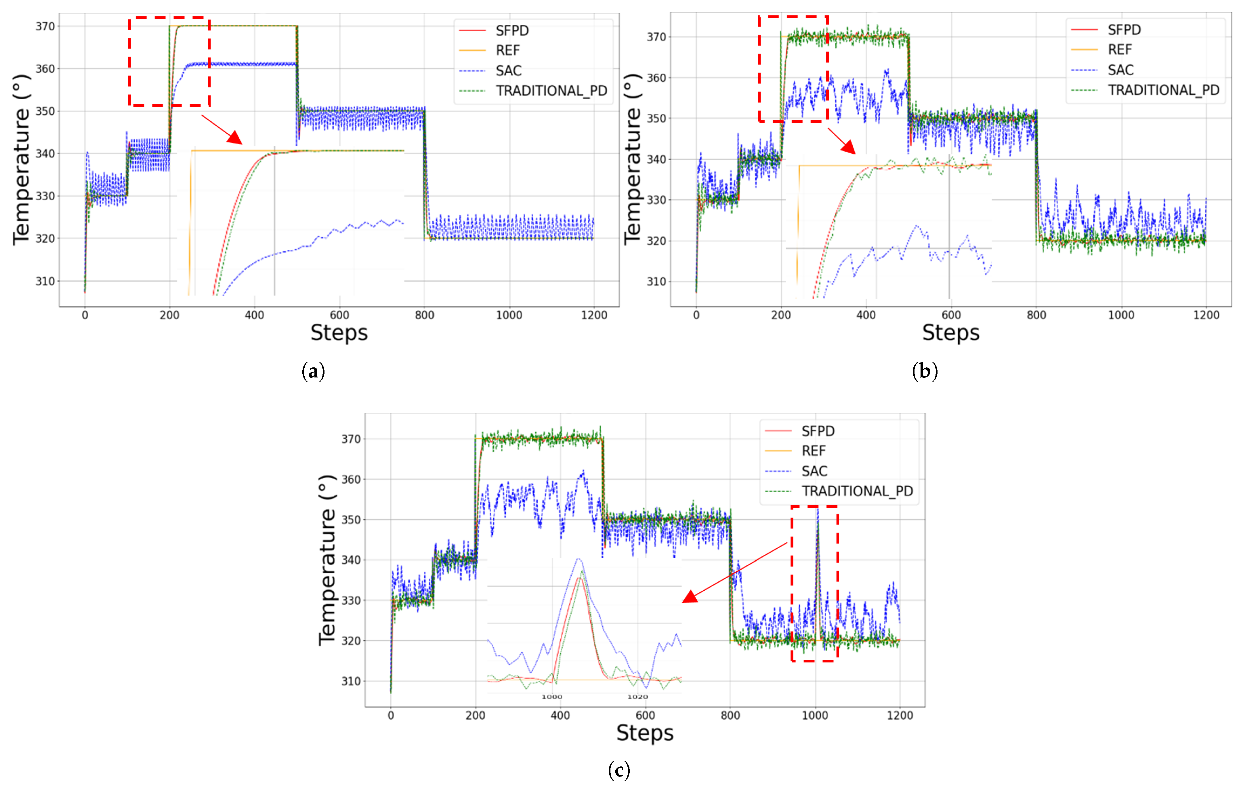
Testing Performance Evaluation
4.3. Complexity Analysis
4.3.1. Space Complexity Analysis
- For the input layer, the space required to store the input data x, where there are n input features, is .
- In the fuzzification layer, each input computes j fuzzy membership values (since there are j fuzzy membership functions per input). The total space required for these fuzzy membership values is .
- In the multiplication layer (fuzzy inference), we store the fuzzy inference result for each rule. With m rules, the space complexity is .
- The normalization layer generates a new vector , requiring space to store the values.
- The defuzzification layer calculates the output , and for r outputs, the space required is .
4.3.2. Time Complexity Analysis
- In the input layer, applying the tanh function to each input element has a time complexity of . For n input features, the overall time complexity is .
- In the fuzzification layer, we compute j fuzzy membership values for each input , and each computation takes time. Therefore, for i inputs and j memberships, the total time complexity is .
- The multiplication layer (fuzzy inference) calculates the fuzzy inference result for each rule by multiplying n fuzzy memberships. The time complexity for each rule is , and for m rules, the total time complexity is .
- The normalization layer involves summing m fuzzy inference results and normalizing each , which takes time.
- The defuzzification layer computes the output , with a time complexity of , as there are r outputs requiring summation of m values.
5. Conclusions
Author Contributions
Funding
Institutional Review Board Statement
Informed Consent Statement
Data Availability Statement
Conflicts of Interest
References
- Li, Y.; Ang, K.H.; Chong, G.C. Patents, software, and hardware for PID control: An overview and analysis of the current art. IEEE Control. Syst. Mag. 2006, 26, 42–54. [Google Scholar]
- Tang, K.S.; Man, K.F.; Chen, G.; Kwong, S. An optimal fuzzy PID controller. IEEE Trans. Ind. Electron. 2001, 48, 757–765. [Google Scholar] [CrossRef]
- Zhou, X.; Xu, C. Fuzzy-PID-based trajectory tracking for 3WIS robot. In Proceedings of the International Conference on Mechatronic Engineering and Artificial Intelligence (MEAI 2023), Shenyang, China, 15–17 December 2023; SPIE: Bellingham, WA, USA, 2024; Volume 13071, pp. 826–834. [Google Scholar]
- Liu, B.; Li, J.; Zhou, X.; Li, X. Design of brushless DC motor simulation action system based on Fuzzy PID. In Proceedings of the Ninth International Symposium on Sensors, Mechatronics, and Automation System (ISSMAS 2023), Nanjing, China, 11–13 August 2023; SPIE: Bellingham, WA, USA, 2024; Volume 12981, pp. 276–280. [Google Scholar]
- Ouyang, P.; Acob, J.; Pano, V. PD with sliding mode control for trajectory tracking of robotic system. Robot. Comput. Integr. Manuf. 2014, 30, 189–200. [Google Scholar] [CrossRef]
- Chi, R.; Li, H.; Shen, D.; Hou, Z.; Huang, B. Enhanced P-type control: Indirect adaptive learning from set-point updates. IEEE Trans. Autom. Control 2022, 68, 1600–1613. [Google Scholar] [CrossRef]
- Carvajal, J.; Chen, G.; Ogmen, H. Fuzzy PID controller: Design, performance evaluation, and stability analysis. Inf. Sci. 2000, 123, 249–270. [Google Scholar] [CrossRef]
- Laib, A.; Gharib, M. Design of an Intelligent Cascade Control Scheme Using a Hybrid Adaptive Neuro-Fuzzy PID Controller for the Suppression of Drill String Torsional Vibration. Appl. Sci. 2024, 14, 5225. [Google Scholar] [CrossRef]
- İrgan, H.; Menak, R.; Tan, N. A comparative study on PI-PD controller design using stability region centroid methods for unstable, integrating and resonant systems with time delay. Meas. Control 2025, 58, 245–265. [Google Scholar] [CrossRef]
- Bhattacharjee, D.; Kim, W.; Chattopadhyay, A.; Waser, R.; Rana, V. Multi-valued and fuzzy logic realization using TaOx memristive devices. Sci. Rep. 2018, 8, 8. [Google Scholar] [CrossRef]
- Mudi, R.K.; Pal, N.R. A robust self-tuning scheme for PI-and PD-type fuzzy controllers. IEEE Trans. Fuzzy Syst. 1999, 7, 2–16. [Google Scholar] [CrossRef]
- Kumar, P.; Nema, S.; Padhy, P. Design of Fuzzy Logic based PD Controller using cuckoo optimization for inverted pendulum. In Proceedings of the 2014 IEEE International Conference on Advanced Communications, Control and Computing Technologies, Ramanathapuram, India, 8–10 May 2014; IEEE: New York, NY, USA, 2014; pp. 141–146. [Google Scholar]
- Zhuang, Q.; Xiao, M.; Tao, B.; Cheng, S. Bifurcations control of IS-LM macroeconomic system via PD controller. In Proceedings of the 2021 China Automation Congress (CAC), Beijing, China, 22–24 October 2021; IEEE: New York, NY, USA, 2021; pp. 4565–4570. [Google Scholar]
- Haarnoja, T.; Zhou, A.; Hartikainen, K.; Tucker, G.; Ha, S.; Tan, J.; Kumar, V.; Zhu, H.; Gupta, A.; Abbeel, P.; et al. Soft actor-critic algorithms and applications. arXiv 2018, arXiv:1812.05905. [Google Scholar]
- He, J.; Su, S.; Wang, H.; Chen, F.; Yin, B. Online PID Tuning Strategy for Hydraulic Servo Control Systems via SAC-Based Deep Reinforcement Learning. Machines 2023, 11, 593. [Google Scholar] [CrossRef]
- Yu, X.; Fan, Y.; Xu, S.; Ou, L. A self-adaptive SAC-PID control approach based on reinforcement learning for mobile robots. Int. J. Robust Nonlinear Control 2022, 32, 9625–9643. [Google Scholar] [CrossRef]
- Song, L.; Xu, C.; Hao, L.; Yao, J.; Guo, R. Research on PID parameter tuning and optimization based on SAC-auto for USV path following. J. Mar. Sci. Eng. 2022, 10, 1847. [Google Scholar] [CrossRef]
- Neves, D.E.; Ishitani, L.; do Patrocínio Júnior, Z.K.G. Advances and challenges in learning from experience replay. Artif. Intell. Rev. 2024, 58, 54. [Google Scholar] [CrossRef]
- Di-Castro, S.; Mannor, S.; Di Castro, D. Analysis of stochastic processes through replay buffers. In Proceedings of the International Conference on Machine Learning, Baltimore, MD, USA, 17–23 July 2022; PMLR: New York, NY, USA, 2022; pp. 5039–5060. [Google Scholar]
- Boubertakh, H.; Tadjine, M.; Glorennec, P.Y.; Labiod, S. Tuning fuzzy PD and PI controllers using reinforcement learning. ISA Trans. 2010, 49, 543–551. [Google Scholar] [CrossRef]
- Puriel-Gil, G.; Yu, W.; Sossa, H. Reinforcement learning compensation based PD control for inverted pendulum. In Proceedings of the 2018 15th International Conference on Electrical Engineering, Computing Science and Automatic Control (CCE), Mexico City, Mexico, 5–7 September 2018; IEEE: New York, NY, USA, 2018; pp. 1–6. [Google Scholar]
- Gil, G.P.; Yu, W.; Sossa, H. Reinforcement learning compensation based PD control for a double inverted pendulum. IEEE Lat. Am. Trans. 2019, 17, 323–329. [Google Scholar]
- Shukur, F.; Mosa, S.J.; Raheem, K.M. Optimization of Fuzzy-PD Control for a 3-DOF Robotics Manipulator Using a Back-Propagation Neural Network. Math. Model. Eng. Probl. 2024, 11, 199. [Google Scholar] [CrossRef]
- Reddy, K.H.; Sharma, S.; Prasad, A.; Krishna, S. Neural Network based Fuzzy plus PD Controller for Speed Control in Electric Vehicles. In Proceedings of the 2024 IEEE International Conference on Interdisciplinary Approaches in Technology and Management for Social Innovation (IATMSI), Gwalior, India, 14–16 March 2024; IEEE: New York, NY, USA, 2024; Volume 2, pp. 1–4. [Google Scholar]
- McCutcheon, L.; Fallah, S. Adaptive PD Control using Deep Reinforcement Learning for Local-Remote Teleoperation with Stochastic Time Delays. In Proceedings of the 2023 IEEE/RSJ International Conference on Intelligent Robots and Systems (IROS), Detroit, MI, USA, 1–5 October 2023; IEEE: New York, NY, USA, 2023; pp. 7046–7053. [Google Scholar]
- Kwan, H.K.; Cai, Y. A fuzzy neural network and its application to pattern recognition. IEEE Trans. Fuzzy Syst. 1994, 2, 185–193. [Google Scholar] [CrossRef]
- Dash, P.; Pradhan, A.; Panda, G. A novel fuzzy neural network based distance relaying scheme. IEEE Trans. Power Deliv. 2000, 15, 902–907. [Google Scholar] [CrossRef]
- Sutton, R.S.; Barto, A.G. Reinforcement Learning: An Introduction; A Bradford Book; MIT Press: Cambridge, MA, USA, 2018; pp. 1–2. [Google Scholar]
- Haarnoja, T.; Zhou, A.; Abbeel, P.; Levine, S. Soft actor-critic: Off-policy maximum entropy deep reinforcement learning with a stochastic actor. In Proceedings of the International Conference on Machine Learning, Stockholm, Sweden, 10–15 July 2018; PMLR: New York, NY, USA, 2018; pp. 1861–1870. [Google Scholar]
- Amari, S.i. Backpropagation and stochastic gradient descent method. Neurocomputing 1993, 5, 185–196. [Google Scholar] [CrossRef]
- Kingma, D.P.; Welling, M. Auto-Encoding Variational Bayes. arXiv 2013, arXiv:1312.6114. [Google Scholar]
- Körpeoğlu, S.G.; Filiz, A.; Yıldız, S.G. AI-driven predictions of mathematical problem-solving beliefs: Fuzzy logic, adaptive neuro-fuzzy inference systems, and artificial neural networks. Appl. Sci. 2025, 15, 494. [Google Scholar] [CrossRef]
- Villa-Ávila, E.; Arévalo, P.; Ochoa-Correa, D.; Espinoza, J.L.; Albornoz-Vintimilla, E.; Jurado, F. Improving V2G Systems Performance with Low-Pass Filter and Fuzzy Logic for PV Power Smoothing in Weak Low-Voltage Networks. Appl. Sci. 2025, 15, 1952. [Google Scholar] [CrossRef]
- Lu, W.; Liang, J.; Su, H. Research on Energy-Saving Optimization Method and Intelligent Control of Refrigeration Station Equipment Based on Fuzzy Neural Network. Appl. Sci. 2025, 15, 1077. [Google Scholar] [CrossRef]
- Juang, C.F.; Chen, T.C.; Cheng, W.Y. Speedup of implementing fuzzy neural networks with high-dimensional inputs through parallel processing on graphic processing units. IEEE Trans. Fuzzy Syst. 2011, 19, 717–728. [Google Scholar] [CrossRef]
- Zhang, Y.; Wang, Z.; Tazeddinova, D.; Ebrahimi, F.; Habibi, M.; Safarpour, H. Enhancing active vibration control performances in a smart rotary sandwich thick nanostructure conveying viscous fluid flow by a PD controller. Waves Random Complex Media 2024, 34, 1835–1858. [Google Scholar] [CrossRef]
- Yang, R.; Gao, Y.; Wang, H.; Ni, X. Fuzzy neural network PID control used in Individual blade control. Aerospace 2023, 10, 623. [Google Scholar] [CrossRef]
- Prado, R.; Melo, J.; Oliveira, J.; Neto, A.D. FPGA based implementation of a Fuzzy Neural Network modular architecture for embedded systems. In Proceedings of the The 2012 International Joint Conference on Neural Networks (IJCNN), Brisbane, QLD, Australia, 10–15 June 2012; IEEE: New York, NY, USA, 2012; pp. 1–7. [Google Scholar]
- Anusha, S.; Karpagam, G.; Bhuvaneswarri, E. Comparison of tuning methods of PID controller. Int. J. Manag. Inf. Technol. Eng. 2014, 2, 1–8. [Google Scholar]
- Oh, S.K.; Jang, H.J.; Pedrycz, W. Optimized fuzzy PD cascade controller: A comparative analysis and design. Simul. Model. Pract. Theory 2011, 19, 181–195. [Google Scholar] [CrossRef]
- Chowdhury, M.A.; Al-Wahaibi, S.S.; Lu, Q. Entropy-maximizing TD3-based reinforcement learning for adaptive PID control of dynamical systems. Comput. Chem. Eng. 2023, 178, 108393. [Google Scholar] [CrossRef]
- Chowdhury, M.A.; Lu, Q. A novel entropy-maximizing TD3-based reinforcement learning for automatic PID tuning. In Proceedings of the 2023 American Control Conference (ACC), San Diego, CA, USA, 31 May–2 June 2023; IEEE: New York, NY, USA, 2023; pp. 2763–2768. [Google Scholar]
- Dogru, O.; Velswamy, K.; Ibrahim, F.; Wu, Y.; Sundaramoorthy, A.S.; Huang, B.; Xu, S.; Nixon, M.; Bell, N. Reinforcement learning approach to autonomous PID tuning. Comput. Chem. Eng. 2022, 161, 107760. [Google Scholar] [CrossRef]
- Shi, Q.; Lam, H.K.; Xuan, C.; Chen, M. Adaptive neuro-fuzzy PID controller based on twin delayed deep deterministic policy gradient algorithm. Neurocomputing 2020, 402, 183–194. [Google Scholar] [CrossRef]
- Shuprajhaa, T.; Sujit, S.K.; Srinivasan, K. Reinforcement learning based adaptive PID controller design for control of linear/nonlinear unstable processes. Appl. Soft Comput. 2022, 128, 109450. [Google Scholar] [CrossRef]


| Notation | Description | Case 1: Pendulum | Case 2: CSTR |
|---|---|---|---|
| P | Number of training episodes | 10 | 50 |
| R | Replay buffer size | 20,000 | 20,000 |
| B | Batch size | 32 | 32 |
| A | Action space | [−10, 10] | [50, 420] |
| - | Learning rate | 0.001 | 0.001 |
| - | Length of steps for testing | 200 | 1200 |
| - | Optimizer | Adam | Adam |
| - | P/D parameter range | [−100, 100]/[−20, 20] | [−5, 5]/[−2, 2] |
| Notation | Description | Value |
|---|---|---|
| g | Gravity acceleration | 10 |
| l | The length of the pendulum | 1.0 |
| m | The mass of the pendulum | 1.0 |
| u | The applied torque | [−10,10] |
| The current angle of the pendulum | [] | |
| The current angular velocity of the pendulum | [−8,8] |
| Param | Value | Unit | Description |
|---|---|---|---|
| F | 1 | m³/h | Liquid flow rate in the vessel |
| V | 1 | m³ | Reactor volume |
| R | 1.985875 | kcal/(kmol·K) | Boltzmann’s ideal gas constant |
| −5.960 | kcal/kmol | Heat of chemical reaction | |
| E | 11,843 | kcal/kmol | Activation energy |
| 34,930,800 | 1/h | Pre-exponential nonthermal factor | |
| 500 | kcal/(m³·K) | Density multiplied by heat capacity | |
| 150 | kcal/(K·h) | Overall heat transfer coefficient multiplied by vessel area |
| WGN | SFPD | SAC | Traditional PD | |||
|---|---|---|---|---|---|---|
| ISE | IAE | ISE | IAE | ISE | IAE | |
| No | 104,046 | 1158 | 341,062 | 3062 | 138,813 | 2659 |
| Yes | 108,167 | 1852 | 351,541 | 3267 | 153,669 | 3399 |
| SI | WGN | SFPD | SAC | Traditional PD | |||
|---|---|---|---|---|---|---|---|
| ISE | IAE | ISE | IAE | ISE | IAE | ||
| 0–100 s | No | 1757 | 115 | 2121 | 320 | 1667 | 132 |
| Yes | 1746 | 140 | 3003 | 408 | 1896 | 206 | |
| 100–200 s | No | 252 | 38 | 751 | 230 | 252 | 45 |
| Yes | 272 | 66 | 875 | 242 | 461 | 128 | |
| 200–500 s | No | 4351 | 218 | 30,832 | 2939 | 4349 | 219 |
| Yes | 4539 | 309 | 69,403 | 4449 | 4596 | 462 | |
| 500–800 s | No | 1031 | 78 | 1659 | 512 | 957 | 80 |
| Yes | 1043 | 189 | 3885 | 859 | 1190 | 329 | |
| 800–1200 s | No | 2644 | 122 | 7584 | 1074 | 2622 | 125 |
| Yes | 2777 | 242 | 16,036 | 2008 | 3518 | 520 | |
Disclaimer/Publisher’s Note: The statements, opinions and data contained in all publications are solely those of the individual author(s) and contributor(s) and not of MDPI and/or the editor(s). MDPI and/or the editor(s) disclaim responsibility for any injury to people or property resulting from any ideas, methods, instructions or products referred to in the content. |
© 2025 by the authors. Licensee MDPI, Basel, Switzerland. This article is an open access article distributed under the terms and conditions of the Creative Commons Attribution (CC BY) license (https://creativecommons.org/licenses/by/4.0/).
Share and Cite
Han, Q.; Boussaid, F.; Bennamoun, M. Soft Fuzzy Reinforcement Neural Network Proportional–Derivative Controller. Appl. Sci. 2025, 15, 5071. https://doi.org/10.3390/app15095071
Han Q, Boussaid F, Bennamoun M. Soft Fuzzy Reinforcement Neural Network Proportional–Derivative Controller. Applied Sciences. 2025; 15(9):5071. https://doi.org/10.3390/app15095071
Chicago/Turabian StyleHan, Qiang, Farid Boussaid, and Mohammed Bennamoun. 2025. "Soft Fuzzy Reinforcement Neural Network Proportional–Derivative Controller" Applied Sciences 15, no. 9: 5071. https://doi.org/10.3390/app15095071
APA StyleHan, Q., Boussaid, F., & Bennamoun, M. (2025). Soft Fuzzy Reinforcement Neural Network Proportional–Derivative Controller. Applied Sciences, 15(9), 5071. https://doi.org/10.3390/app15095071