The Pseudoinverse Gradient Descent Method with Eight Branch Directions (8B-PGDM): An Improved Dead Reckoning Algorithm Based on the Local Invariance of Navigation

Abstract

This paper establishes a fundamental connection between the local time invariance of motion parameters and dead reckoning (DR) accuracy. This insight enables the reformulation of navigation parameter estimation as a convex optimization problem solvable through our novel Eight-Branch Pseudoinverse Gradient Descent Method (8B-PGDM). This method addresses non-cooperative positioning challenges in sparse-sensor regimes, particularly enabling real-time trajectory prediction when facing intermittent measurements (e.g., <5 Hz sampling rates) or persistent signal blockages. This method achieves an excellent estimation accuracy with only three samplings and an prediction MSE of $0.7906$, significantly better than traditional dead reckoning (DR) methods. This approach effectively mitigates the impact of data scarcity, enabling robust and accurate trajectory predictions in challenging environments.

1. Introduction

Dead reckoning (DR) is widely adopted for navigation-assisted positioning, autonomous vehicle localization, and robot path planning. However, its performance degrades in non-cooperative scenarios where targets cannot actively provide positioning data, such as wildlife tracking (e.g., marine turtles [1] and migratory species [2]) or uncrewed aerial vehicle navigation [3]. These scenarios face three critical challenges:

• Sparse observations: Targets rarely emit detectable signals [4].
• Resource constraints: Limited energy budgets and narrow communication bandwidths.
• Nonlinear dynamics: Nonlinear motion patterns (e.g., animal behaviors [5]).

Current DR solutions fall into three categories. First is the data-driven trajectory prediction method. Deep learning methods like RNNs [6,7], LSTMs [8], and GCNs [9] have improved sequence modeling by capturing temporal dependencies. While these models achieve higher accuracy than traditional methods, they require large training datasets and struggle with generalization to unseen scenarios [10]. Second is the multi source information fusion strategy. To overcome sparse observations, researchers combine complementary sensing modalities. In order to address the limitations of single sensor data [11,12], scholars have proposed various multi-source information fusion schemes [13], for example, combining visual perception data with IMU data to construct robust state estimation algorithms [14,15]. Alternatively, radar echo features can be integrated with historical trajectory data to enhance the reliability of predictions. While ref. [16] developed a novel inertial-aided Unmodulated Visible Light Positioning system (uLiDR) for resource-constrained platforms like smartphones, ref. [17] further improved accuracy by integrating IMU, magnetic field, Bluetooth, and semantic map data with a robust particle filtering method. This cross-modal information fusion [18] not only improves the reliability of prediction results, but also alleviates the problem of sparse observation data to a certain extent. Third is dynamic modeling and optimization. This is crucial to establish an accurate dynamic model for the motion characteristics of noncooperative targets. Animals’ movement patterns often have strong randomness and uncertainty, as discussed in refs. [5,19,20]. For aircraft, UGVs, or boats, the influence of aerodynamics or fluid dynamics needs to be considered. By conducting an in-depth analysis of the motion law of the target object [21] and combining it with optimal control theory [22], the effectiveness of trajectory prediction can be significantly improved.

However, in this application context, existing dead reckoning methods face three core bottlenecks:

• High-frequency data dependence: traditional inertial navigation systems (INS) require IMU sampling rates above 10 Hz to suppress integral drift, but in noncooperative scenarios, target observation frequencies are often lower than 5 Hz (such as satellite remote sensing revisit periods), leading to the failure of conventional Kalman filtering frameworks.
• Dynamic model mismatch: existing methods often assume that the target follows a linear motion model, but in fact, ships often perform nonlinear avoidance maneuvers [23].
• Obstacles to multi-source heterogeneous data fusion include spatiotemporal asynchrony and coordinate system homogeneity in multimodal data such as radar, AIS, EO/IR in non cooperative scenarios.

This study develops a novel motion-invariance-driven framework for parameter estimation and trajectory prediction that fundamentally addresses three critical challenges in navigation systems: (1) dependency on high-frequency sampling, (2) nonlinear maneuver prediction limitations, and (3) strict spatiotemporal synchronization requirements. Our primary innovations encompass three fundamental advancements.

• Theoretical Foundation: We establish the first formal connection between motion invariance principles and dead reckoning methodologies through Lie group analysis. This theoretical bridge enables the derivation of system observability conditions under sparse sampling regimes.
• Algorithmic Breakthrough: An innovative methodology is established that leverages geometric invariants to reformulate the original non-convex parameter estimation problem into a tractable convex optimization framework.
• Engineering Implementation: The proposed dual-stage predictor-corrector architecture achieves continuous trajectory prediction.

The rest of this article is organized as follows: In Section 2, we establish the basic relationship between the local time invariance of motion parameters and the accuracy of dead reckoning (DR) and use some properties and assumptions to transform the problem of time-invariant parameter solving into a convex optimization problem. In Section 3, we use the pseudo inverse gradient descent method to solve convex optimization problems and analyze and discuss the convergence domain and convergence. Finally, we propose an eight-branch pseudo inverse gradient descent method (8B-PGDM). In Section 4, we design experiments to validate the effectiveness of our method and then compare it with traditional DR methods to demonstrate its advantages and usage limitations. Finally, we have made some comments in Section 5 to conclude this article.

2. Problem Formulation and Modeling

The purpose of this section is to elaborate on the research model and the key issues to be addressed. Firstly, the core principle of motion invariant parameters is introduced from the classic DR algorithm. Then, taking the motion object controlled by the optimal guidance law as an example, the expected state of the control is taken as its invariant parameter. In order to estimate the invariant parameter, the geometric properties of the motion trajectory are analyzed, and the convex optimization form of the problem is obtained from the geometric properties.

DR usually speculates on the state of motion at some point in the future based on the current estimated state of motion $\Delta t$. Usually, its standard form is Equation (1), where the vector P denotes the state of motion, $\dot{P}$ denotes the speed (first derivative of the state of motion), and $\ddot{P}$ denotes the acceleration (second derivative of the state of motion). All the variables used in mathematical formulas in the following text are listed in Table 1.

$$\mathbf{P}(t_0+\delta t)=\mathbf{P}\left(t_0\right)+\dot{\mathbf{P}}\left(t_0\right)\Delta t+{\displaystyle \frac{1}{2}}\ddot{\mathbf{P}}\left(t_0\right)\Delta t^2+\cdots$$

(1)

Table 1. Symbols and notations used in this paper.

Symbol	Description
$\mathbf{P}\left(t\right)$	Position vector in global coordinates
${\left[R\right]}_{w\to b}$	Rotation matrix from world frame to body frame
$\Phi$	Rotation vector (axis-angle representation)
$\Omega$	Skew-symmetric matrix of angular velocity
$V_b$, $A_b$	Linear velocity/acceleration in body frame
$\Delta t$	Discrete time step increment
$\dot{(·)}$	Time derivative operator
J	Total cost function
$\Theta (·)$	Terminal state error penalty
$F(·)$	Energy consumption function
X	State vector
A, B	Coefficients for calculating intersection coordinates of two parametric circles.
U	Control input vector
$x_f,y_f$	Expected endpoint coordinate position on a 2-D coordinate plane
$q\left(t\right)$	Bearing angle: ${tan}^{-1}{\displaystyle \frac{y_f-y\left(t\right)}{x_f-x\left(t\right)}}$
r	Radial distance: $\sqrt{{(x_f-x\left(t\right))}^2+{(y_f-y\left(t\right))}^2}$
${\theta }_f$	Final desired heading angle
$t_0$, $t_f$	Initial and final time instants
$\tau$	Integration time variable

2.1. Time-Invariance of Motion Parameters

At the beginning, an aircraft is employed as a representative case to investigate which parameters are treated as invariant during motion state extrapolation. Furthermore, a systematic evaluation of the benefits and limitations associated with these invariant parameters in dead reckoning applications is presented.

Let $P_0$ be the position vector of the extrapolation reference point in the world coordinate system, let $V_b$ be the velocity vector in the body coordinate system, and let $A_b$ represent the tangential acceleration. $\Omega$ is the skew-symmetric matrix form (Lie algebra) of the angular velocity vector. The corresponding DR algorithm is shown in Equation (2). Obviously, $V_b$, $A_b$, and $\Omega$ are the default invariants in dead reckoning algorithms.

$$\begin{array}{cc}\hfill {\left[R\right]}_{w->b}& =e^{[\Phi (t_0+\Delta t)]}{\left[R_o\right]}_{w->b}\hfill \end{array}$$

(2a)

$$\begin{array}{cc}\hfill P(t_0+\Delta t)& =P_o+{\left[R\right]}_{w->b}^{-1}\underset{\mathrm{displacement}\mathrm{relative}\mathrm{to}{P}_0^{*}\mathrm{at}{t}_0+\Delta t}{\underbrace{\left({\int }_0^{\Delta t}{e}^{\tau \Omega }{V}_{b}d\tau +{\int }_0^{\Delta t}\tau e^{\tau \Omega }{A}_{b}d\tau \right)}}\hfill \end{array}$$

(2b)

Among them, the exponential mapping in Equation (2a) is expanded as follows:

$$e^{[\Phi (t_0+\Delta t)]}=cos\left(\right|\omega |\Delta t)I+(1-cos(\left|\omega \right|\Delta t\left)\right){\displaystyle \frac{\omega {\omega }^T}{{\left|\omega \right|}^2}}-{\displaystyle \frac{sin\left|\omega \right|\Delta t}{\left|\omega \right|}}\Omega$$

By setting a fixed state synchronization period to correct the dead reckoning error, a three-dimensional space track and dead reckoning trajectory can be obtained, as shown in Figure 1. The red trajectory curve is the actual motion path of the aircraft. The continuous yellow line segments are the predicted (extrapolated) trajectories at equal time intervals. The segments where the transition from the yellow to the red trajectories occurs are the hard synchronizations when the error threshold is surpassed.

Figure 1. DR algorithm applied to the aircraft. The red trajectory curve is the actual trajectory of the aircraft. The continuous yellow lines are the extrapolated segments at equal time intervals.

By projecting the trajectory onto a plane consisting of the vertical and x-axis, Figure 2 can be obtained, and the relationship between the line segments (the blue dashed lines) and the smooth trajectory (the black curves) calculated according to the second-order dead position can be seen. It can be seen that after the imminent large overload maneuver at $x=$ 18,000 m, the maximum deviation in the vertical direction of dead reckoning reaches 75 m because the acceleration in the vertical direction is changing rapidly, even in reverse.

Figure 2. Comparison of the 2nd-order extrapolation DR algorithm in the orthometric height coordinate system (HCS) to the real trajectory. The black solid line represents the actual flight trajectory, the blue dashed line represents the trajectory segment calculated by second-order dead reckoning, the red hollow circle represents the position during hard synchronization, and the double headed arrow represents the maximum error vector of each extrapolated trajectory segment.

The sources of error are also analyzed. Since velocity and acceleration are simply considered as constants during actual motion, when the time span is large, the deviation can easily exceed the allowable range; i.e., the invariance of the selected parameters is poor. Therefore, one way to improve the dead reckoning method is to select a parameter with better invariance for dead reckoning. In most cases, the higher the order of the motion parameters, the more sensitive to the measurement noise, and the lower the order of the motion parameters, the worse the invariance. For a controlled object, there is one potential parameter with relatively good time-invariance, and that is the desired end state of motion. When the parameter is taken in the control law as a motion parameter with good time-invariance, a better dead reckoning result may be obtained.

2.2. Time-Invariant Parameters in Optimal Control

When choosing a class of control laws as a reference, we give preference to optimal control. Optimal control is common and representative in nature and practical engineering applications. In practical engineering in the aerospace field, spacecraft orbit transfer relies on optimal control to determine the optimal thrust direction and magnitude, minimize fuel consumption and mission time, and enable spacecraft attitude control. Aircraft flight control uses optimal control to optimize flight trajectories, fuel consumption, and time. We use the following assumptions to standardize the dead reckoning objects discussed next.

Assumption 1.

Moving entities possess the capabilities of route planning and motion control.

Assumption 2.

The moving entity can independently establish the desired target state $x\left(t_f\right)$ on its own. However, it will not take the initiative to notify the observing side.

Assumption 3.

The entity (autonomous mobile robots or drones) adopts optimal control in the motion planning of the flight route (continuous state control). Let the entity state be $x\in {\mathbb{R}}^n$, the control input be $u\in {\mathbb{R}}^p$, and the corresponding state equation be $\dot{X}=f(x,u,t)$. The performance index of the optimal state control is described as follows:

$$J=\underset{\mathrm{End}\mathrm{state}\mathrm{error}}{\underbrace{\Theta \left[x\left(t_f\right),t_f\right]}}+\underset{\mathrm{Energy}\mathrm{consumption}}{\underbrace{{\int }_{t_0}^{t_f}F(x,u,t)dt}}$$

(3)

where $\Theta (·)$ and $F(·)$ are scalar functions, representing the positive definite expressions of the state error and the input, respectively.

To facilitate the analysis and discussion, it is better to simplify the problem to the optimal guidance control in a two-dimensional plane. In Figure 3, the position at time t, namely $x\left(t\right),y\left(t\right)$, is located at the lower left corner. The angle between the moving velocity V and the horizontal axis of the coordinate system is ${\theta }_t$. The azimuth angle $q_t$ is formed by the desired waypoint $x\left(t_f\right),y\left(t_f\right)$ relative to the current position of the moving entity, and ${\theta }_f$ represents the velocity direction constraint when reaching the desired position in the constraints.

$$\left\{\begin{array}{c}\dot{r}=-V·cos(\theta -q\left(t\right))\hfill \\ r\dot{q}=-V·sin(\theta -q\left(t\right))\hfill \end{array}\right.$$

(4)

where

$$q\left(t\right)=ta{n}^{-1}{\displaystyle \frac{y\left(t_f\right)-y\left(t\right)}{x\left(t_f\right)-x\left(t\right)}}$$

and

$$r=\sqrt{{(y\left(t_f\right)-y\left(t\right))}^2+{(x\left(t_f\right)-x\left(t\right))}^2}$$

Figure 3. Schematic diagram of navigation guidance parameters in a two-dimensional plane.

Let $x_1={\theta }_f-q$, $x_2=\dot{q}$; it can be obtained that

$$\left\{\begin{array}{c}{\dot{x}}_1=-x_2\hfill \\ {\dot{x}}_2=(-2\dot{r}/r)x_2+(\dot{r}/r)\dot{\theta }\hfill \end{array}\right.$$

(5)

Set $X={\left[\begin{array}{cc}{x}_1& x_2\end{array}\right]}^T$, $A=\left[\begin{array}{cc}0& -1\\ 0& -2\dot{r}/r\end{array}\right]$, $B={\left[\begin{array}{cc}0& \dot{r}/r\end{array}\right]}^T$, and $U\left(t\right)=\dot{\theta }$; thus, the state-space expression of the control system can be obtained,

$$\left\{\begin{array}{c}\dot{X}=AX+BU\hfill \\ X\left(t_f\right)=0\hfill \end{array}\right.$$

(6)

The scalar functions of $\theta (·)$ and $F(·)$ in Equation (3) are designed as matrices of parameters Q and R of quadratic functional functions and the indicator becomes

$$J=X^T\left(t_f\right)QX\left(t_f\right)+{\int }_{t_0}^{t_f}{U}^T\left(t\right)RU\left(t\right)dt$$

(7)

To solve the optimal control problem of a second-order system using Pontryagin’s Minimum Principle, the control law should take the following form,

$$U\left(t\right)=-R^{-1}{B}^{T}PX$$

(8)

The optimal guidance law corresponding to the solution of the Riccati equation based on the parameter matrix Q and R should take the following form in Equation (9):

$$\dot{\theta }=\underset{\mathrm{Move}\mathrm{to}{x}_f,y_f}{\underbrace{\mu ·\dot{q}}}+\underset{\mathrm{Rotate}\mathrm{to}{\theta }_f}{\underbrace{\lambda ({\theta }_f-q)·{\displaystyle \frac{\dot{r}}{r}}}}$$

(9)

It can be clearly observed that the moving object under optimal guidance control states $x\left(t_f\right),y\left(t_f\right)$, and ${\theta }_f$ has parameters with stable time-invariant characteristics. However, since Equation (9) is not a convex function, the expected final state cannot be estimated by the least squares method.

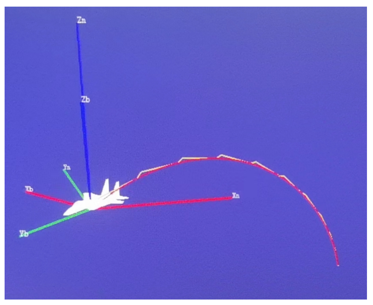
2.3. Geometric Properties of Trajectory

Therefore, by analyzing its geometric properties, the problem can be converted into a convex function that can be solved. Use a classic math trick, we multiply both sides of Equation (9) by $r^2$ and then substitute it into Equation (4); the following equation can be obtained.

$${(x_f-(x\left(t\right)-{\displaystyle \frac{b}{2\dot{\theta }}}))}^2+{(y_f-(y\left(t\right)-{\displaystyle \frac{d}{2\dot{\theta }}}))}^2={\displaystyle \frac{b^2+d^2}{4{\dot{\theta }}^2}}$$

(10)

where b and d are, respectively,

$$\begin{array}{cc}\hfill b& =V(\mu ·sin\left(\theta \left(t\right)\right)+\lambda ({\theta }_f-q\left(t\right))·cos\left(\theta \left(t\right)\right))\hfill \end{array}$$

(11a)

$$\begin{array}{cc}\hfill d& =V(-\mu ·cos\left(\theta \left(t\right)\right)+\lambda ({\theta }_f-q\left(t\right))·sin\left(\theta \left(t\right)\right))\hfill \end{array}$$

(11b)

To simplify the expression in Equation (10), we define $x_f\triangleq x\left(t_f\right),y_f\triangleq y\left(t_f\right),{\theta }_f\triangleq \theta \left(t_f\right)$, and $q\left(t\right)=ta{n}^{-1}{\displaystyle \frac{y_f-y\left(t\right)}{x_f-x\left(t\right)}}$.

The conventional method is to select $t_i\in (t_0,t),i=1,2,3$ before t at the current moment to obtain Equation (10) by solving a system of nonlinear equations, solving for $x_f,y_f,{\theta }_f$, three unknowns. However, the problem is, in fact, that it is not possible to obtain a convergent solution by directly applying Newton’s method, L-M solver, etc. (experimental test), and it is necessary to first transform the solution problem into a reasonable optimization problem (preferably a convex optimization problem).

Continuing to work on Equation (10), it is obvious that for any selection of $t\in \left(t_0,t_f\right]$, there is a parametric circle with the coordinates of the center of the circle $(x_c,y_c)$, where $x_c=x\left(t\right)-{\displaystyle \frac{b}{2\dot{\theta }}}$ and $y_c=y\left(t\right)-{\displaystyle \frac{d}{2\dot{\theta }}}$, and the radius of the circle is $r={\displaystyle \frac{\sqrt{b^2+d^2}}{2|\dot{\theta }|}}$, and the circle intersects the trajectory line at $(x_t,y_t)$ and $(x_f,y_f)$. Literally, if the parameter circle corresponding to a sampling point intersects the trajectory line at the desired endpoint, then the parameter circle corresponding to two different sampling points must intersect at the desired endpoint together. Thus, its geometric properties can be generalized as follows.

Property 1.

The parameter circles of any sample points on the trajectory line are intersected at the same point.

Property 2.

The same point at which the parametric circles intersect is the desired final state position.

To characterize the aforementioned properties, a representative trajectory is analyzed with sampling instants defined at $t=0.001,15.001,30.001$ s. The constructed parameter circles in Figure 4 demonstrate two critical geometric features: (i) All circles intersect the trajectory precisely at both the sampled instants and the terminal waypoint $(x_f,y_f)$; (ii) these circles exhibit a common intersection point at $(x_f,y_f)$, confirming the geometric invariance predicted by Property 2.

Figure 4. The points on the 1st, 15,001st and 30,001st trajectory lines were taken as sampling points, and the parameter circles were obtained.

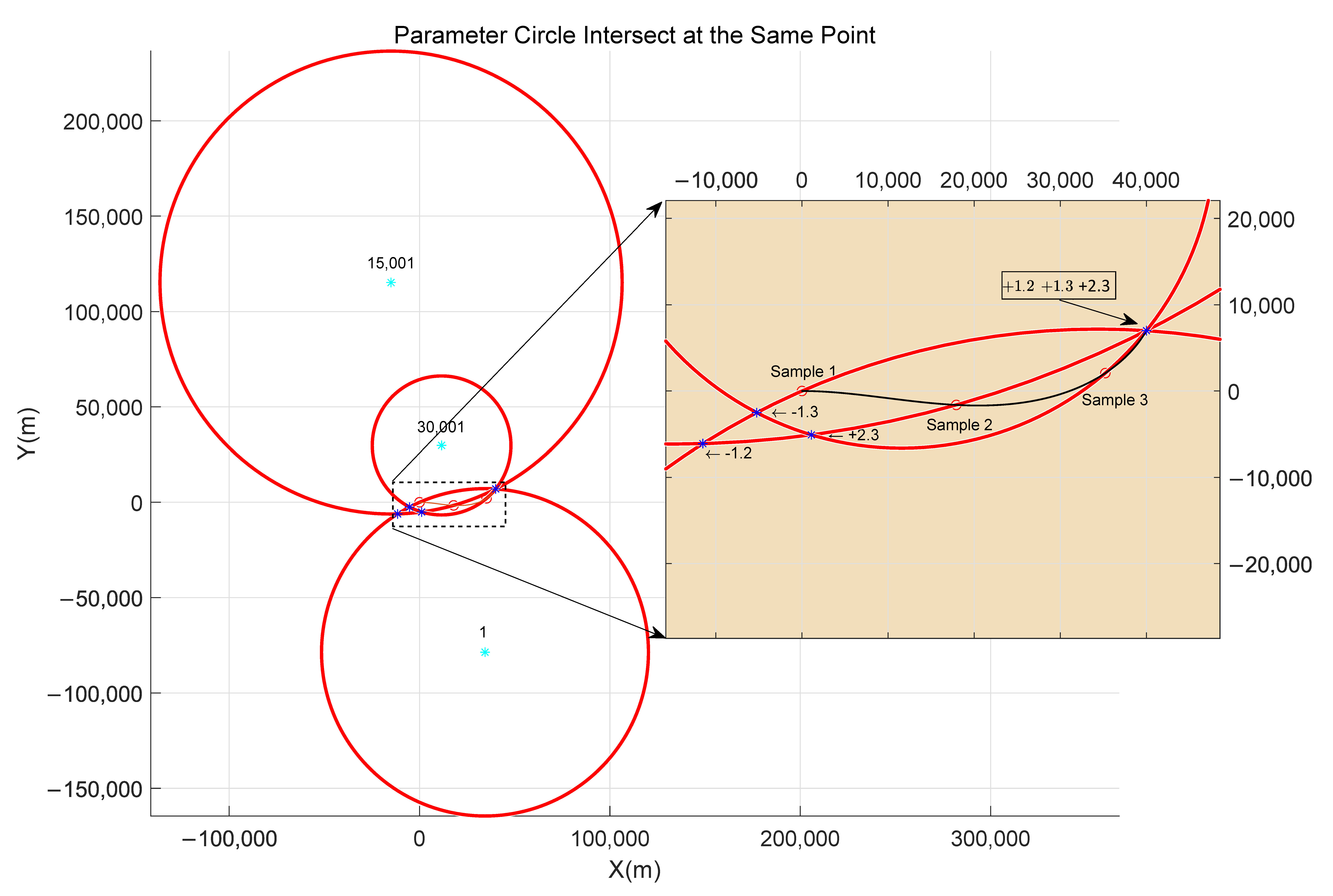
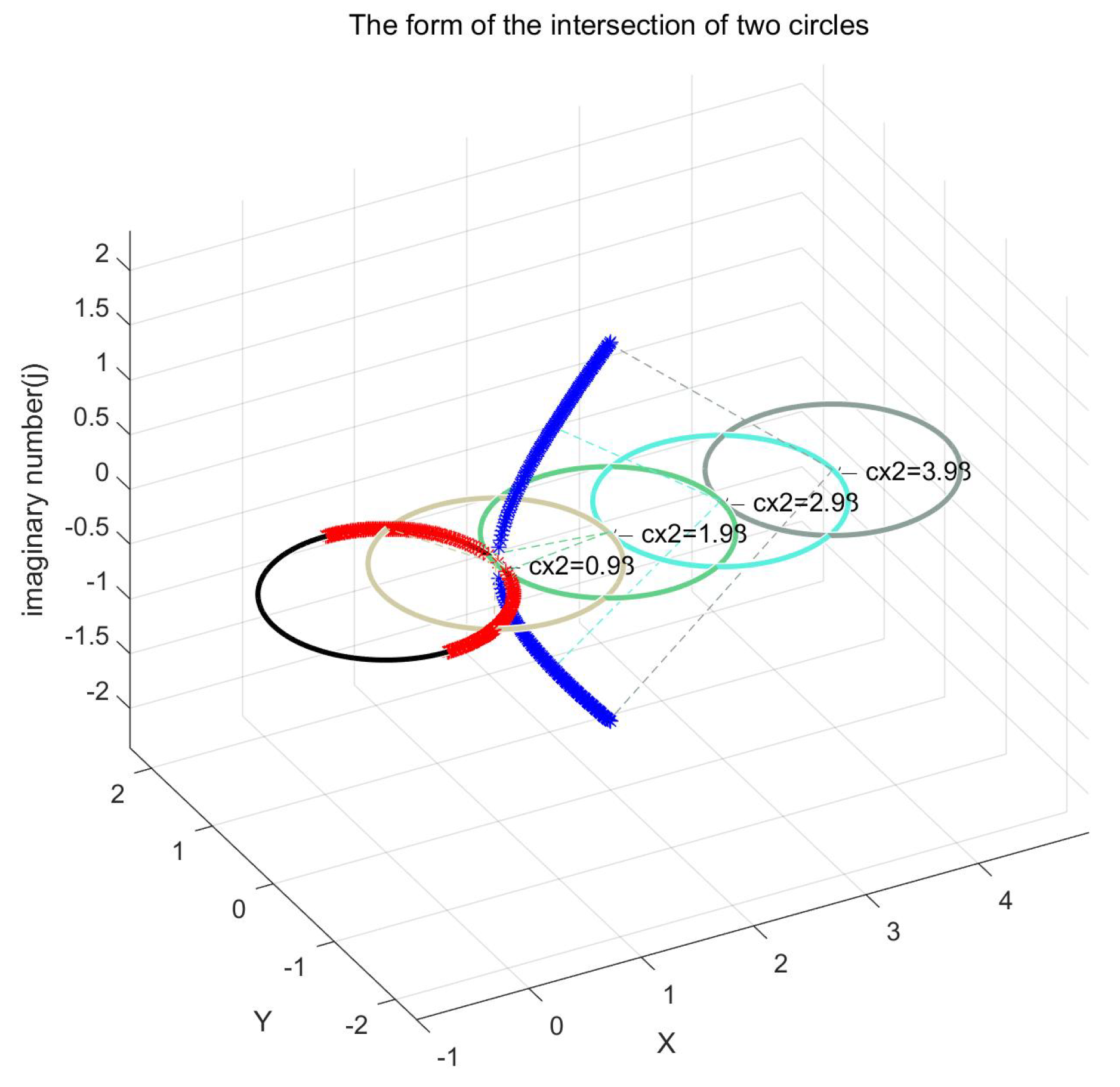
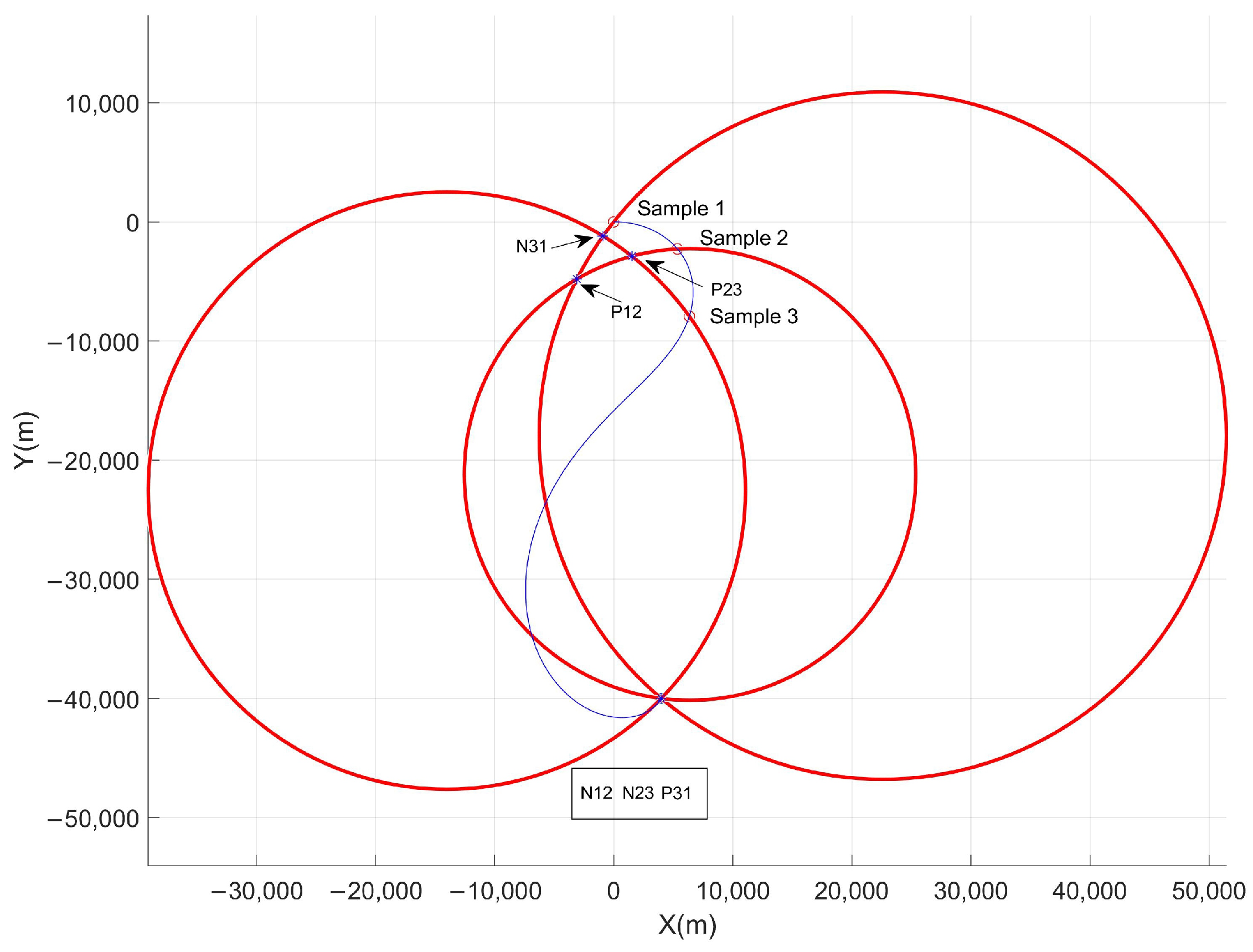
2.4. Convex Function Construction

In order to solve for the time-invariant parameter of the desired final state, we construct a convex function using property 1, in which parametric circles intersect at the same point.

Firstly, the analytical solution of the intersection of two parameter circles is studied. For two sampling moments $t_1$ and $t_2$, there are two parameter circles. Suppose the centers of the two circles are at ${(}^1{x}_c{,}^2{x}_c)$ and ${(}^2{x}_c{,}^2{x}_c)$, and the radii are ${}^{1}r_c$ and ${}^{2}r_c$, respectively. Thus, the midpoint between the two parameter circles is $\mathbf{O}=({\displaystyle \frac{{}^{1}x_c+{}^{2}x_c}{2}},{\displaystyle \frac{{}^{1}y_c+{}^{2}y_c}{2}})$, and we define L as the distance in between and take the unit basis vector ${\mathbf{e}}_a=({\displaystyle \frac{{}^{2}x_c-{}^{1}x_c}{L}},{\displaystyle \frac{{}^{2}y_c-{}^{1}y_c}{L}})$ in the direction from one circle’s center to another, while the orthogonal unit basis vector is ${\mathbf{e}}_b=({\displaystyle \frac{{}^{2}y_c-{}^{1}y_c}{L}},-{\displaystyle \frac{{}^{2}x_c-{}^{1}x_c}{L}})$. Thus, the analytic solution of the two intersections in Equation (12) can be obtained.

$$\left\{\begin{array}{c}{\mathbf{J}}_{1,2}^{+}=\mathbf{O}+A·{\mathbf{e}}_a+B·{\mathbf{e}}_b\hfill \\ {\mathbf{J}}_{1,2}^{-}=\mathbf{O}+A·{\mathbf{e}}_a-B·{\mathbf{e}}_b\hfill \end{array}\right.$$

(12)

where

$$A={\displaystyle \frac{{}^{1}r_c^2-{}^{2}r_c^2}{2L}}$$

and

$$B={\displaystyle \frac{1}{2L}}\sqrt{-[{{(}^1{r}_c{+}^2{r}_c)}^2-L^2][{{(}^1{r}_c{-}^2{r}_c)}^2-L^2]}$$

In terms of the form of the analytical solution, there may be no intersections, i.e., imaginary roots, as shown in Figure 5. Therefore, the search space may not be limited to the real domain space ${\mathbb{R}}^3$, and in order for the algorithm to run robustly, the problem should be extended to the unitary space ${\mathbb{C}}^3$ in Section 3.

Figure 5. The form of the intersection is affected by the parametric circle (there may be 2 intersections, 1 double root, or a conjugated double root).

The process of solving for $x_f^{*},y_f^{*},$ and ${\theta }_f^{*}$ is regarded as the optimal estimation of the parameters. Once these values are obtained, they are substituted into Equation (10), which allows us to obtain the set of three parametric circles ${\mathbb{P}}_c=\left\{{(}^i{x}_c{,}^i{y}_c{,}^i{r}_c)\right|i=1,2,3\}$ for $t_i\in (t_0,t),i=1,2,3$ with $t_i\in (t_0,t),i=1,2,3$. There are up to six intersections between the three circles on the $xOy$ plane, and according to the geometry of the problem, three of them intersect on the trajectory line at the desired end point of the trajectory. If any two parametric circles from them are chosen, say those corresponding to indices i and j, there will be two intersection points $J_{i,j}^{+}$ and $J_{i,j}^{-}$, which constitute the geometric properties of the system. It is preferable to use binary $s_i$ (where the symbol + represents the positive root and the symbol − represents the negative root) to represent and define the intersection point combinations simultaneously. It can be observed that there is a ${\displaystyle \frac{1}{2}}$ probability of selecting the potential common point (end point of the trajectory) from the intersection points provided by each pair of circles. Consequently, there are eight possible combinations of the intersection points that are selected (“+++”, “++−”, “+−+”, “+−−”, “−++”, “−+−”, “−−+”, “−−−”).

$${\mathbb{C}}_{s_2,s_1,s_0}=\{J_{1,2}^{s_2},J_{2,3}^{s_1},J_{3,1}^{s_0}\},s_i\in \{+,-\}$$

(13)

Nevertheless, only a unique combination within the set ${\mathbb{C}}_{s_2,s_1,s_0}$ satisfies the optimization criteria. This is demonstrated as follows. (i) Property 1, which establishes the intersection condition between parametric circles and their common point $(x_f,y_f)$, where the first term of the objective function in Equation (14) corresponds to the 2-norm of geometric congruence errors; (ii) Property 2, which specifies that $(x_f,y_f)$ coincides with the trajectory’s terminal waypoint, where the second 2-norm term quantifies terminal state deviation.

$$V_{s_2,s_1,s_0}=\underset{V^o:\mathrm{Norm}\mathrm{with}\mathrm{other}\mathrm{intersecions}}{{\displaystyle \underbrace{\sum _{J_{i,j}^s,J_{j,k}^s\in {\mathbb{C}}_{s_2,s_1,s_0}}{\displaystyle \frac{1}{2}}\left|\right|J_{i,j}^s-J_{i,j}^s{\left|\right|}^2}}}+\underset{V^d:\mathrm{Norm}\mathrm{with}\mathrm{desired}\mathrm{position}}{{\displaystyle \underbrace{\sum _{J_{i,j}^s\in {\mathbb{C}}_{s_2,s_1,s_0}}{\displaystyle \frac{1}{2}}\left|\right|(x_f,y_f)-J_{i,j}^s{\left|\right|}^2}}}$$

(14)

Thus, the parameter estimation problem becomes the one shown in Equation (15), which is solved so that the sum of two sqares of the 2-norms is taken as the smallest combination $s_2,s_1,s_0$ of intersection points $J_{1,2}^{s_2},J_{2,3}^{s_1},J_{3,1}^{s_0}$ and the corresponding target end state $x_f,y_f,$ and ${\theta }_f$. Obviously, the optimization goal V is positively definite, and if $\dot{V}$ is negatively definite, and the problem model is a convex optimization problem; this would ensure that any local minimum is also a global minimum.

Thus, the optimization problem for parameter estimation takes the form shown in Equation (15). That is, the sum of the distances between the intersections is minimal, and the sum of the distances between the intersections and the final state positions is also minimal. To make the sum of squares of the norm representing the distances equal to 0, two conditions need to be met simultaneously: 1. the selected intersection group $J_{1,2}^{s_2},J_{2,3}^{s_1},J_{3,1}^{s_0}$ is correct; 2. the solution is precisely the corresponding target ending states $x_f,y_f,$ and ${\theta }_f$.

$$arg\underset{x_f,y_f,{\theta }_f}{min}{V}_{s_2,s_1,s_0}=arg\underset{x_f,y_f,{\theta }_f}{min}(V^d+V^o)$$

(15)

3. Methods

As mentioned in the previous section, there are a total of 8 possible branches that need to be optimized and iterated to find the final optimal solution, so the Pseudoinverse Gradient Descent Method with Eight Branch Directions (8B-PGDM) is proposed. Since V is the sum of two sqares of the 2-norms, it is obviously a convex function. Assuming that the intersections can be extended to unitary space, then it is not affected by the undefined imaginary intersection point, and the variable $x_f^{*},,y_f^{*},{\theta }_f^{*}\in \mathbb{R}$ can be considered unconstrained. Then, the optimization objective function V is a convex optimization problem. Since it is a convex optimization problem, common optimization solvers, such as Pseudoinverse Gradient Descent Method can be used to solve the problem.

3.1. Pseudoinverse Gradient Descent Method

Considering that the optimization target V is positively definite, then, as long as the appropriate $\delta x_f^{*},\delta y_f^{*},\delta {\theta }_f^{*}$ is taken to make $\Delta V(x_f^{*},y_f^{*},{\theta }_f^{*})$ negatively determined, then it can converge asymptotically to 0 according to Lyapunov’s theorem. The existence of the optimal solution is proven. Based on this existence result, a method named Pseudoinverse Gradient Descent Method (PGDM) is developed, which leverages the properties of the problem. Specifically, the existence of the optimal solution guarantees that the algorithm has a theoretical target to converge to. Additionally, by exploiting the convergence properties of the solution, the update rules, step size adjustment strategies, and termination conditions of PGDM are designed to ensure that it can efficiently find the optimal solution.

Since the dimension of ${[\delta x_f^{*},\delta y_f^{*},\delta {\theta }_f^{*}]}^T$ is 3, we need at least 3 linearly independent equations to find the inverse of the relevant matrix in order to solve for these unknowns. To this end, $V_d$ and $V_o$ are considered to be expanded in terms of the X and Y axes by expressing them as functions of the components on the X and Y axes through projection. Then, by taking derivatives of these functions with respect to ${[\delta x_f^{*},\delta y_f^{*},\delta {\theta }_f^{*}]}^T$, a system of equations can be obtained. If the resulting coefficient matrix of this system of equations is not invertible, the Moore–Penrose pseudoinverse can be adopted to solve for the optimized gradient direction. This is because the pseudoinverse provides a least-squares solution, which is particularly useful when dealing with overdetermined or underdetermined systems of equations.

$$\left[\begin{array}{c}\delta x_f^{*}\\ \delta y_f^{*}\\ \delta {\theta }_f^{*}\end{array}\right]=-{\left[\begin{array}{ccc}{\displaystyle \frac{\partial V_x^d}{\partial x_f^{*}}}& {\displaystyle \frac{\partial V_x^d}{\partial y_f^{*}}}& {\displaystyle \frac{\partial V_x^d}{\partial {\theta }_f^{*}}}\\ {\displaystyle \frac{\partial V_y^d}{\partial x_f^{*}}}& {\displaystyle \frac{\partial V_y^d}{\partial y_f^{*}}}& {\displaystyle \frac{\partial V_y^d}{\partial {\theta }_f^{*}}}\\ {\displaystyle \frac{\partial V_x^o}{\partial x_f^{*}}}& {\displaystyle \frac{\partial V_x^o}{\partial y_f^{*}}}& {\displaystyle \frac{\partial V_x^o}{\partial {\theta }_f^{*}}}\\ {\displaystyle \frac{\partial V_x^o}{\partial x_f^{*}}}& {\displaystyle \frac{\partial V_x^o}{\partial y_f^{*}}}& {\displaystyle \frac{\partial V_x^o}{\partial {\theta }_f^{*}}}\end{array}\right]}^{+}·\left[\begin{array}{c}{V}_x^d\\ V_y^d\\ V_x^o\\ V_x^o\end{array}\right]$$

(16)

According to the situation of the current branch, the pseudoinverse of the Jacobian matrix at the current iterative solution of the Lyapunov function is used to perform a local linearization operation on the function. On this basis, the gradient iterative vector $[\delta x_f^{*},\delta y_f^{*},\delta {\theta }_f^{*}]$ is further obtained to make the error asymptotically converge, as shown in Equation (17). ${[V_x^d,V_y^d,V_x^o,V_x^o]}^T$ is the projection component vector of the objective functions $V^d$ and $V^o$ at ${[x_f^{*},y_f^{*},{\theta }_f^{*}]}_k$. Thus, the solution for the next iteration is defined by Equation (17).

$${[x_f^{*},y_f^{*},{\theta }_f^{*}]}_{k+1}={[x_f^{*},y_f^{*},{\theta }_f^{*}]}_k+[\delta x_f^{*},\delta y_f^{*},\delta {\theta }_f^{*}]$$

(17)

where ${[x_f^{*},y_f^{*},{\theta }_f^{*}]}_k$ is the parameter vector of the k-th iteration.

3.2. Intermediate Complexity of Methods

During iterative solution procedures, scenarios may arise where parametric circles lack intersection points, necessitating an analysis of complex roots. To address this, the concept of complex root distance is formalized in Definition 2. The algorithm strategically expands the solution space through intermediate complex-number embeddings, as detailed in Algorithm 1. Crucially, real-domain feasibility is enforced through a mapping operator that projects complex-valued iteration vectors back into real space. This mechanism exemplifies the Intermediate-Complexity Principle: while complex-number operations are permitted during transient computational phases, all terminal solutions are constrained to real-space coordinates.

Definition 1 (Distance in a Unitary Space).

Let $V_u$ be a unitary space over the complex field $\mathbb{C}$ with an inner product $⟨·,·⟩:V_u\times V_u\to \mathbb{C}$ that satisfies the following properties:

• For all $u,v,w\in V_u$ and $a,b\in \mathbb{C}$, $⟨au+bv,w⟩=a⟨u,w⟩+b⟨v,w⟩$ (linearity).
• $⟨u,v⟩=\overline{⟨v,u⟩}$ (conjugate symmetry), where $\overline{⟨v,u⟩}$ denotes the complex conjugate of $⟨v,u⟩$.
• For all $u\in V_u$, $⟨u,u⟩\ge 0$ and $⟨u,u⟩=0$ if and only if $u=0$ (positive definiteness).

Definition 2.

The distance $d(u,v)$ between two vectors $u,v\in V_u$ is defined as $d(u,v)=\parallel u-v\parallel$, where the norm $\parallel u\parallel$ of a vector u is given by $\parallel u\parallel =\sqrt{⟨u,u⟩}$. In the case of an n-dimensional unitary space $V_u={\mathbb{C}}^n$ with the standard inner product $⟨u,v⟩={\sum }_{i=1}^n{u}_i\overline{v_i}$, the distance formula can be explicitly written as $d(u,v)=\sqrt{{\sum }_{i=1}^n(u_i-v_i)\overline{(u_i-v_i)}}$.

Algorithm 1 Iterative Optimization Solver for 8B-PGDM

1: Initialize ${[x_f^{*},y_f^{*},{\theta }_f^{*}]}_0$ (Initial guess) 2: Set $ϵ=5$ (Error tolerance) 3: Set $k=0$(iteration counter) 4: Set maximum number of iterations $N_{max}$ 5: while $k<N_{max}$ and $V>ϵ$ do 6:    for all $s_2,s_1,s_0\in \{+,-\}$ do 7:         Compute $[\delta x_f^{*},\delta y_f^{*},\delta {\theta }_f^{*}]$—Equation (16) 8:         Update $[x_f^{*},y_f^{*},{\theta }_f^{*}]\leftarrow [x_f^{*},y_f^{*},{\theta }_f^{*}]+[\delta x_f^{*},\delta y_f^{*},\delta {\theta }_f^{*}]$ 9:         Compute $V_{s_2,s_1,s_0}$—Equation (14) 10:    end for 11:    $V=min\left(V_{s_2,s_1,s_0}\right)$ 12:    $k=k+1$ 13: end while 14: Return $x_f,y_f,{\theta }_f$ and $s_2,s_1,s_0$

Next, assuming that the current branch is about the intersection of $J_{1,2}^{+},J_{2,3}^{+}$, and $J_{3,1}^{+}$, we will take the elements in the Jacobian matrix as an example to demonstrate how to extend the method to the complex root.

According to the chain rule, we have the partial derivative item ${\displaystyle \frac{\partial V_x^d}{\partial x_f^{*}}}$ in the Jacobian matrix. In the following formula, we use two important symbols, ℜ and ℑ, related to complex numbers. The symbol $\Re \left(z\right)$ represents the real part, and the symbol $\Im \left(z\right)$ represents the imaginary part of a complex number $z=\Re \left(z\right)+i\Im \left(z\right)$. The distance $d(u,v)$ in Definition 2 can be expressed as $d^2(u,v)={\Re }^2(u-v)+{\Im }^2(u-v)$. Let $x_{i,j}^{+}$ represent the x-axis projection component of $J_{i,j}^{+}$.

$$\begin{array}{cc}\hfill {\displaystyle \frac{\partial V_x^d}{\partial x_f^{*}}}& ={\displaystyle \frac{1}{2}}\sum _{i\ne j}^{i,j}{\displaystyle \frac{\partial ({(x_f^{*}-\Re \left(x_{i,j}^{+}\right))}^2+{\Im }^2\left(x_{i,j}^{+}\right))}{\partial x_f^{*}}}\hfill \\ \hfill & =\sum _{i\ne j}^{i,j}(x_f^{*}-\Re \left(x_{i,j}^{+}\right))(1-{\displaystyle \frac{\partial \Re \left(x_{i,j}^{+}\right)}{\partial x_f^{*}}})+\Im \left(x_{i,j}^{+}\right){\displaystyle \frac{\partial \Im \left(x_{i,j}^{+}\right)}{\partial x_f^{*}}}\hfill \end{array}$$

(18)

As for ${\displaystyle \frac{\partial \Re \left(x_{i,j}^{+}\right)}{\partial x_f^{*}}}$ and ${\displaystyle \frac{\partial \Im \left(x_{i,j}^{+}\right)}{\partial x_f^{*}}}$, they can be obtained by substituting Equation (12) and projecting $\mathbf{O},{\mathbf{e}}_a$ and ${\mathbf{e}}_b$ on the x-axis.

$${\displaystyle \frac{\partial \Re \left(x_{i,j}^{+}\right)}{\partial x_f^{*}}}={\displaystyle \frac{\partial (\frac{{}^{i}x_c+{}^{j}x_c}{2}+A·\frac{{}^{j}x_c-{}^{i}x_c}{L}+\Re \left(B\right)·\frac{{}^{j}y_c-{}^{i}y_c}{L})}{\partial x_f^{*}}}$$

(19)

$${\displaystyle \frac{\partial \Im \left(x_{i,j}^{+}\right)}{\partial x_f^{*}}}={\displaystyle \frac{\partial (\Im \left(B\right)·\frac{{}^{j}y_c-{}^{i}y_c}{L})}{\partial x_f^{*}}}$$

(20)

Next, to get the full form of the partial derivative, it needs to substitute ${\displaystyle \frac{{\partial }^i{x}_c}{\partial x_f^{*}}},{\displaystyle \frac{{\partial }^i{y}_c}{\partial x_f^{*}}},{\displaystyle \frac{{\partial }^i{r}_c}{\partial x_f^{*}}}$ from Equation (11a,b) into the above equation.

3.3. Convergence Analysis

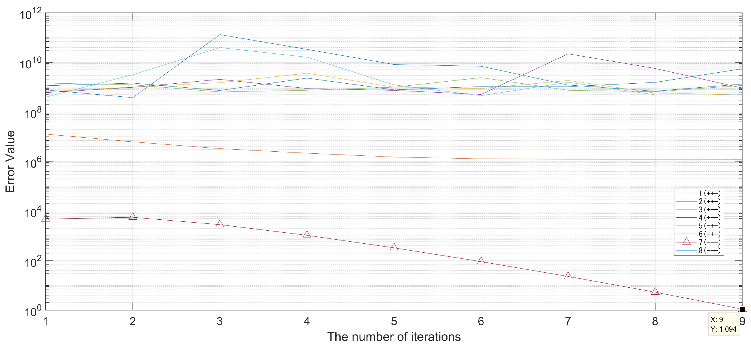
As explained at the beginning of this section, this problem is a convex optimization problem, and in order to ensure that the optimal solution can be approximated in the iterative solution process, it is necessary to use the derivative of the Lyapunov function to prove the convergence of the error.

The negative definite property of the derivative of the Lyapunov function can be obtained by its Definition 3.

Definition 3

(Lyapunov Function Derivative in Discrete Time Systems). Let $x_k\in {\mathbb{R}}^n$ be the state vector at the k-th iteration of a discrete-time dynamical system, and $g:{\mathbb{R}}^n\to {\mathbb{R}}^n$ be the state transition function such that $x_{k+1}=g\left(x_k\right)$. Given a Lyapunov function $V\left(x\right):{\mathbb{R}}^n\to \mathbb{R}$, its derivative is approximated as follows. Let ${\mathbf{J}}_V\left(x\right)$ be the Jacobian matrix of $V\left(x\right)$, which is a $1\times n$ row vector with elements ${\mathbf{J}}_V\left(x\right)=\left[{\displaystyle \frac{\partial V}{\partial x_1}},{\displaystyle \frac{\partial V}{\partial x_2}},\cdots ,{\displaystyle \frac{\partial V}{\partial x_n}}\right]$. The derivative of the Lyapunov function, denoted by $\dot{V}\left(x_k\right)$, is defined as

$$\dot{V}\left(x_k\right)\approx V\left(x_{k+1}\right)-V\left(x_k\right)$$

By using the Taylor expansion of $V\left(g\right(x\left)\right)$ at $x=x_k$, and letting $\Delta x\triangleq g\left(x_k\right)-x_k$, there is

$$\begin{array}{cc}\hfill V\left(x_{k+1}\right)& =V\left(g\left(x_k\right)\right)\hfill \\ \hfill & \approx V\left(x_k\right)+{\mathbf{J}}_V\left(x_k\right)(\Delta x)+{O(\parallel \Delta x\parallel }^2)\hfill \end{array}$$

(21)

Thus, the first-order approximation of the Lyapunov function derivative is given by

$$\dot{V}\left(x_k\right)\approx {\mathbf{J}}_V\left(x_k\right)(g\left(x_k\right)-x_k)$$

(22)

From the full differentiation of Equation (14), there is the form of the derivative of the Lyapunov function $\dot{V}\left({\mathbf{x}}_k\right)$. Substituting Equation (16) into Equation (22) and still allowing ${\mathbf{x}}_k$ to represent the vector ${[x_f^{*},y_f^{*},{\theta }_f^{*}]}_k$] gives the derivative of the Lyapunov function, as shown in the following equation.

$$\begin{array}{cc}\hfill \dot{V}\left({\mathbf{x}}_k\right)& \approx V_x^d·▵V_x^d+V_y^d·▵V_y^d+V_x^o·▵V_x^o+V_x^o·▵V_x^o\hfill \\ \hfill & \approx \left[\begin{array}{c}{V}_x^d,V_y^d,V_x^o,V_x^o\end{array}\right]{\mathbf{J}}_V\left({\mathbf{x}}_k\right)(g\left({\mathbf{x}}_k\right)-{\mathbf{x}}_k)\hfill \\ \hfill & \approx {\left[\begin{array}{c}{V}_x^d\\ V_y^d\\ V_x^o\\ V_x^o\end{array}\right]}^T{\mathbf{J}}_V\left(x_k\right)·-{\mathbf{J}}_V{\left(x_k\right)}^{+}\left[\begin{array}{c}{V}_x^d\\ V_y^d\\ V_x^o\\ V_x^o\end{array}\right]\hfill \\ \hfill & \approx -({\left(V_x^d\right)}^2+{\left(V_y^d\right)}^2+{\left(V_x^o\right)}^2+{\left(V_x^o\right)}^2)\le 0\hfill \end{array}$$

(23)

At this point, the convergence has been proven.

3.4. 8B-PGDM

In the problem description and modeling section, the analysis has shown that there are 8 branches in the combination of intersections, and only one of them can obtain the optimal estimate of the final state through iterative optimization due to the uniqueness of the solution required by geometric properties. We will elaborate on the optimization solution algorithm logic below in the case of 8 branches (Algorithm 1).

Initialization Step: The algorithm starts by setting up the necessary initial conditions. In general, first-order extrapolation can be used for the most recent sample points to obtain the initial state of the solution vector ${[x_f^{*},y_f^{*},{\theta }_f^{*}]}_0$ to be optimized. Considering the actual computing power and real-time requirements, the error tolerance $ϵ$ and maximum iteration count $N_{max}$ are also defined as stopping criteria.

Iterative Process: The ‘while’ loop ensures that the algorithm continues until either the maximum number of iterations is reached or the error tolerance is met. The ‘for’ loop allows the algorithm to explore different configurations of $s_2,s_1,s_0\in \{+,-\}$, which might represent different combinations of intersections in the optimization problem. The computation of $[\delta x_f^{*},\delta y_f^{*},\delta {\theta }_f^{*}]$ using Equation (16) is the key step in updating the parameters ${[x_f^{*},y_f^{*},{\theta }_f^{*}]}_k$ in the direction of optimization. The subsequent update step modifies the parameters based on these increments. The computation of $V_{s_2,s_1,s_0}$ using Equation (14) will evaluate the objective function (a Lyapunov-like function) associated with the optimization problem. The minimum value of $V_{s_2,s_1,s_0}$ is selected on behalf of the error as the optimal solution among the eight branches.

Termination and Output: By judging whether the optimal solution in the 8 branches meets the convergence requirements ($V<ϵ$), the iterative solution process is terminated. The stopping criterion $k>N_{max}$ ensures that the algorithm does not run indefinitely. Upon termination, the algorithm outputs the optimized values $V_{s_2,s_1,s_0}$ of the parameters $[x_f^{*},y_f^{*},{\theta }_f^{*}]$, which represent the solution found by the optimization process.

4. Results

To ensure the validity and reliability of these results, a well-designed experimental setup was employed. Here are the results obtained from experiments and analyses.

4.1. Design of Experiments

Configuration of experimental conditions: In the experiment, it is assumed that there is a cruise missile whose initial position is at the origin $(0,0)$, whose attitude is parallel to the horizontal axis ($\theta =0$), and whose constant velocity $v=400$, with optimal control law parameters $\mu =4,\lambda =2$, and the flight under optimal guidance is performed to the desired position (4000, −40,000) and the desired attitude of $\pi$/3 rad. For numerical simulation, continuous simulations were performed with a simulation step size of 1 ms for a total of 300 s.

Control group settings for the experimental method: We employed four different methods as a control group in experiment; they are the first-order Dead Reckoning Algorithm (first-order DR) and second-order Dead Reckoning Algorithm (second-order DR). For the first-order DR and second-order DR methods, two different experimental conditions were set up. In the first condition, the update period was fixed at 1 s, and in the second condition, the update was triggered based on an error threshold of 10 m, while 8B-PGDM was tested based on three sampling points at $0.001$ s, $15.001$ s and $30.001$ s, without specifying an update period or error threshold.

4.2. Method Validation

To verify the method proposed, the experimental design was structured in the following way. Firstly, a continuous system simulation was employed to obtain the motion trajectory under optimal guidance control (blue curves in Figure 6). Then, based on three sampling points, the 8B-PGDM method was applied, and the eight branches were optimized and iterated synchronously, and from the error convergence decline in Figure 7, it can be seen that the logarithmic curve of the seventh (–+) iterative error converges to the lowest point, and the corresponding cases of the branch line are the negative intersection of the first parameter circle and the second parameter circle ($s_2=-$), the negative intersection point of the second parameter circle and the third parameter circle ($s_1=-$), the orthogonal point of the third parameter circle and the first parameter circle ($s_0=+$), and the error function (Lyapunov) when the termination condition occurs converges to $1.094$. In contrast, the other branches do not have an optimal solution where the error converges to within the 0 neighborhood. And the estimated values of the parameter vector $[x_f^{*},y_f^{*},{\theta }_f^{*}]$ are [3998, −39,999, 1.0471].

Figure 6. Numerical simulation of trajectory parameterization via geometric circle constraints (blue: predicted trajectory; red rings: sampling points at $\Delta t=\{0.001\mathrm{s},15.001\mathrm{s},30.001\mathrm{s}\}$; dashed black: solved parameter circles intersecting at the target endpoint $(x=4000,y=-4\times {10}^4)$).

Figure 7. The 8-Branch Pseudogradient Descent Method. Only branch 7 in red line decorated with triangles that corresponding to the situation “$s_2,s_1,s_0=--+$” asynchronous convergence to reach the termination threshold with $ϵ=1.094$ after 9 iterations.

At this point, effectiveness has been verified, which can determine the intersection point combination of parameter circles and the corresponding motion state estimation parameters in the process of the synchronous optimization of eight branches. In addition, the optimal solution was reached in only nine iteration cycles, and the convergence speed was fast.

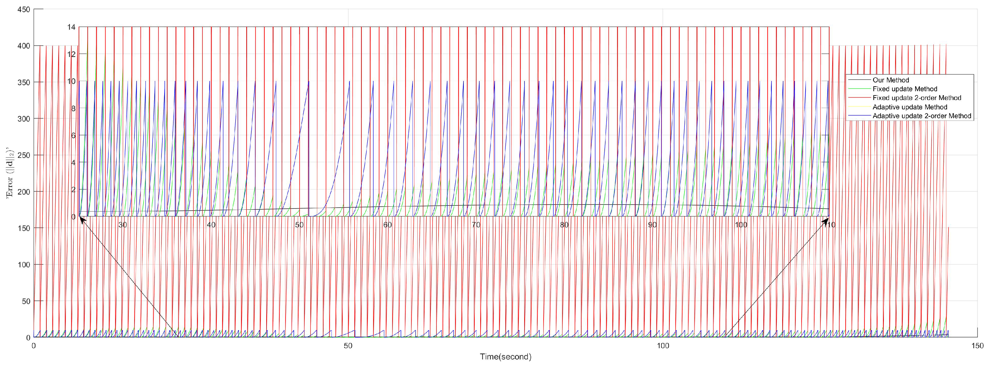
4.3. Performance Comparison

The following presents an analysis of the experimental results obtained from the different methods evaluated in the study. As shown in Table 2, several methods are compared, including the proposed method (8B-PGDM) and different orders of dead reckoning (DR) methods under various conditions.

Table 2. Comparison of the experimental results of different methods.

Method	Update Criterion	Samples	MSE	${\mathit{R}}^2$ in X	${\mathit{R}}^2$ in Y	STD
8B-PGDM	-	3	0.7906	$1.0000$	$1.0000$	$0.8892$
1st-order DR	1 s	146	18.053	$1.0000$	$1.0000$	$4.2489$
2nd-order DR	1 s	146	53176	$0.9977$	$0.9997$	$230.5974$
1st-order DR	$ϵ>10$ m	122	19.913	$1.0000$	$1.0000$	$4.4623$
2nd-order DR	$ϵ>10$ m	122	19.913	$1.0000$	$1.0000$	$4.4623$

For the method 8B-PGDM, according to the parameter estimation ($x_f^{*}=3998,y_f^{*}=-\mathrm{39,999},$${\theta }_f^{*}=1.0471$ rad) obtained by the 8B-PGDM, the flight trajectory of the missile can be obtained by introducing the guidance law of the formula in Equation (24) to an inner continuous system simulation process as per Equation (4).

$$\begin{array}{cc}\hfill \dot{\theta }& =4·\dot{q}+2(1.0471-q)·{\displaystyle \frac{\dot{r}}{r}}\hfill \\ \hfill q\left(0\right)& =ta{n}^{-1}{\displaystyle \frac{-\mathrm{39,999}-y\left(0\right)}{3998-x\left(0\right)}}\hfill \\ \hfill r\left(0\right)& =\sqrt{{3998}^2+{(-\mathrm{39,999})}^2}\hfill \end{array}$$

(24)

As for the control group, the current state is estimated by extrapolation in the same way as the step size 1 ms of the continuous system simulation, and the motion state of the object is obtained through observation or communication only when the update condition is triggered (threshold ≤ 10 m or T = 1 s).

The Mean Squared Error (MSE) values of different methods provide crucial insights into their performance. As shown in Table 2, the proposed method, 8B-PGDM, achieves an MSE of $0.94459$, which is remarkably lower than those of the other methods. In contrast, the first-order DR method shows varying MSE values depending on the update criteria. When the update criterion is a fixed period of 1 s, the MSE is $18.053$. However, when the update is triggered by the condition, the MSE increases slightly to $19.913$. The second-order DR method exhibits a significantly higher MSE of 53176 when the update criterion is a fixed period of 1 s, suggesting poor performance under this condition. Interestingly, when the update is based on the condition, the second-order DR method has the same MSE as the first-order DR method under the same condition, with a value of $19.913$. This comparison indicates that the 8B-PGDM method outperforms both the first and second-order DR methods in terms of minimizing the MSE, regardless of the update criteria. The large MSE of the second-order DR method under the fixed 1 s update criterion might imply that the second-order approximation is not effective under this setting. Meanwhile, the similar MSE of both first and second-order DR methods under this condition suggests that the order of approximation may not be the sole factor influencing the MSE, and other factors related to the update criteria could have a more significant impact.

The number of samples required by each method also reveals important information about their computational cost, observation, and communication needs. As presented in Table 2, the 8B-PGDM method uses only three samples, which is considerably fewer than the sample times of the other methods. The first and second-order DR methods both require 146 samples when the update criterion is a fixed period of 1 s, indicating a higher computational cost associated with this update strategy. When the update is based on this condition ($ϵ>10$ m), both methods use 122 samples, showing that the error-based update criteria reduce the number of samples required compared to the fixed 1 s update criteria. The substantial difference in sample times between the 8B-PGDM method and the DR methods suggests that the 8B-PGDM method is more efficient in terms of computational cost, especially considering its relatively low MSE. The fact that the DR methods require more samples, especially under the fixed 1 s update criteria, implies that more frequent sampling might be necessary to maintain a certain level of performance, whereas the 8B-PGDM method can achieve good performance with far fewer samples.

In summary, compared with other traditional methods in Figure 8, our method has the advantage of having fewer sampling times, smooth curve estimation, and small cumulative error.

Figure 8. Comparison of 8B-PGDM with traditional methods.

4.4. Limitations

The current method still exhibits several shortcomings in research. Firstly, it necessitates parallel iterative optimization across the eight branches. This not only augments the computational complexity but also imposes higher demands on hardware capabilities for parallel processing, thereby potentially restricting its practical applicability in resource-constrained environments. Such a requirement could pose challenges in systems with limited computational resources, impeding its seamless integration and deployment. Secondly, the method is strictly tailored to the corresponding guidance law, with the precondition that certain parameters, specifically mu and lambda, must be known. This inherent constraint significantly limits the method’s universality. In real-world scenarios, accurately obtaining these parameters can be quite challenging, and moreover, the guidance law might vary depending on diverse mission requirements. This lack of flexibility may undermine the method’s versatility and applicability in different operational contexts. Thirdly, a sensitivity analysis of this method regarding the noise present in the observations has not been performed. In practical applications, noise is an inescapable factor, and neglecting its influence can lead to inaccurate results and a degradation in the algorithm’s reliability. Consequently, future research efforts should be concentrated on addressing these issues to enhance the method’s overall effectiveness and practicality, thereby facilitating its broader adoption and more reliable performance under various conditions.

5. Conclusions

This paper conducts an in-depth analysis of the relationship between the local time invariance of motion parameters and the performance of the corresponding dead-reckoning algorithm. Given the awareness that the expected state exhibits superior time invariance compared to the temporary state, a geometric approach is devised. This approach transforms the parameter-estimation problem into a convex optimization problem. To solve the optimization problem and accurately estimate the expected state, a pseudoinverse gradient descent method featuring eight branch directions is employed. The proposed 8B-PGDM achieves excellent estimation accuracy with only three samplings, with an MSE of 0.7906, significantly better than traditional dead reckoning (DR) methods.

In terms of effectiveness and significance, the following aspects can be highlighted. Firstly, the method is capable of achieving trajectory predictions with fewer sampling times, which is particularly advantageous in scenarios where the target is occluded or communication is intermittent. This feature enables the method to operate effectively under challenging conditions, ensuring reliable performance even when data acquisition is limited. Secondly, it can yield trajectory predictions with a smaller mean squared error. A lower mean squared error indicates a higher accuracy of the predictions, thereby improving the overall quality and reliability of the results obtained through the method. Thirdly, the predicted trajectories are smooth without jaggedness. Smooth trajectories are more desirable in many applications as they conform better to physical realities and are easier to interpret and utilize, enhancing the practical value of the predicted results. Finally, the iterative solution speed of the method is fast. Rapid iteration enables quick convergence and timely results, making the method suitable for time-sensitive applications where real-time or near-real-time processing is required, thereby enhancing its efficiency and responsiveness in dynamic situations.

6. Future Work

For the next steps, the following plans are envisioned. Firstly, a sensitivity analysis of the method will be conducted regarding the noise present in the observations. This analysis aims to investigate how the method’s performance is affected by different levels and types of noise, providing valuable insights into its robustness and reliability under noisy conditions. Secondly, generalization studies will be carried out on other motion patterns and the time invariance of their associated parameters. By exploring a wider range of motion patterns, the applicability of the method is expected to be extended, and the understanding of time-invariance properties in various dynamic systems is anticipated to be deepened, which could potentially lead to more comprehensive and versatile models. Finally, an attempt will be made to transform the method into a neural network unit. This unit is designed for the online identification of motion types and parameters, followed by online prediction. The neural network architecture leverages its powerful learning and generalization capabilities to continuously adapt to different motion characteristics, enabling real-time motion recognition and prediction, thereby enhancing the method’s utility in dynamic and complex environments.

References

- Gogendeau, P.; Bonhommeau, S.; Fourati, H.; Oliveira, D.D.; Taillandier, V.; Goharzadeh, A.; Bernard, S. Dead-reckoning configurations analysis for marine turtle context in a controlled environment. IEEE Sens. J. 2022, 22, 12298–12306. [Google Scholar] [CrossRef]
- Kuang, J.; Liu, T.; Wang, Y.; Meng, X.; Niu, X. Magnetic vector constraint pedestrian dead reckoning based on foot-mounted and waist-mounted imu. IEEE Internet Things J. 2025. [Google Scholar] [CrossRef]
- Vaughan, D. Dead Reckoning: Air Traffic Control, System Effects and Risk; University of Chicago Press: Chicago, IL, USA, 2021; ISBN 978-0-226-82032-3. [Google Scholar]
- Mori, D.; Kamekawa, M.; Fujieda, N.; Mizuno, Y. Robust vehicle state estimation from urban driving to the limits of handling. IEEE Trans. Intelligent Transp. Syst. 2024, 26, 892–905. [Google Scholar] [CrossRef]
- Gunner, R.M.; Holton, M.D.; Scantlebury, D.M.; Hopkins, P.; Shepard, E.L.; Fell, A.J.; Garde, B.; Quintana, F.; Gómez-Laich, A.; Yoda, K.; et al. How often should dead-reckoned animal movement paths be corrected for drift? Anim. Biotelemetry 2021, 9, 43. [Google Scholar] [CrossRef] [PubMed]
- Feigl, T.; Kram, S.; Woller, P.; Siddiqui, R.H.; Philippsen, M.; Mutschler, C. Rnn-aided human velocity estimation from a single imu. Sensors 2020, 20, 3656. [Google Scholar] [CrossRef]
- Canbek, K.O.; Yalcin, H.; Baran, E.A. Drift compensation of a holonomic mobile robot using recurrent neural networks. Intell. Serv. Robot. 2022, 15, 399–409. [Google Scholar] [CrossRef]
- Toskovic, A.; Petrovic, A.; Jovanovic, L.; Bacanin, N.; Zivkovic, M.; Dobrojevic, M. Marine Vessel Trajectory Forecasting Using Long Short-Term Memory Neural Networks Optimized via Modified Metaheuristic Algorithm; AIS Algorithms for Intelligent Systems; Springer: Singapore, 2024; pp. 51–66. [Google Scholar]
- Lin, J.; Zou, C.; Lan, L.; Gu, S.; An, X. Deep heading estimation for pedestrian dead reckoning. J. Phys. Conf. Ser. 2020, 1656, 012009. [Google Scholar] [CrossRef]
- Hurwitz, D.; Cohen, N.; Klein, I. Deep-learning-assisted inertial dead reckoning and fusion. IEEE Trans. Instrum. Meas. 2025, 74, 2501009. [Google Scholar] [CrossRef]
- Brossard, M.; Barrau, A.; Bonnabel, S. Ai-imu dead-reckoning. IEEE Trans. Intell. Veh. 2020, 5, 585–595. [Google Scholar] [CrossRef]
- Liu, X.; Zhang, Y.; Li, N.; Huang, Y.; Zhao, Y. A novel pedestrian dead-reckoning algorithm with self-estimates of imu biases. IEEE Trans. Instrumentation Meas. 2025, 74, 8503709. [Google Scholar] [CrossRef]
- Niu, Z.; Cong, L.; Qin, H.; Cao, S. Pedestrian dead reckoning based on complex motion mode recognition using hierarchical classification. IEEE Sens. J. 2024, 24, 4935–4947. [Google Scholar] [CrossRef]
- Li, H.; Guo, H.; Qi, Y.; Deng, L.; Yu, M. Research on multi-sensor pedestrian dead reckoning method with ukf algorithm. Measurement 2021, 169, 108524. [Google Scholar] [CrossRef]
- Li, L.; Wei, Z.; Zhang, T.; Cai, D. Three-dimensional dead reckoning of wall-climbing robot based on information fusion of compound extended kalman filter. J. Field Robot. 2023, 40, 505–520. [Google Scholar] [CrossRef]
- Yang, X.; Zhang, H.; Zhuang, Y.; Wang, Y.; Shi, M.; Xu, Y. ulidr: An inertial-assisted unmodulated visible light positioning system for smartphone-based pedestrian navigation. Inf. Fusion 2025, 113, 102579. [Google Scholar] [CrossRef]
- Yang, X.; Huang, X.; Zhang, Y.; Liu, Z.; Pang, Y. Multi-sensor fusion and semantic map-based particle filtering for robust indoor localization. Measurement 2025, 242, 115874. [Google Scholar] [CrossRef]
- Wu, L.; Guo, S.; Han, L.; Anil Baris, C. Indoor positioning method for pedestrian dead reckoning based on multi-source sensors. Measurement 2024, 229, 114416. [Google Scholar] [CrossRef]
- Lin, F.; Cai, Q.; Liu, Y.; Chen, Y.; Huang, J.; Peng, H. Pedestrian dead reckoning method based on array imu. IEEE Sens. J. 2024, 24, 37753–37763. [Google Scholar] [CrossRef]
- Bergmann, X.H.J. Rocip: Robust continuous inertial position tracking for complex actions emerging from the interaction of human actors and environment. Appl. Intell. 2025, 55, 494. [Google Scholar]
- Ji, S.; Zhang, C.; Tian, L.; Ran, L.; Yang, Y. Dead reckoning method for tracking wellbore trajectories constrained by the drill pipe length. IEEE Trans. Instrum. Meas. 2024, 73, 8509512. [Google Scholar] [CrossRef]
- Chai, R.; Chen, K.; Hua, B.; Lu, Y.; Xia, Y.; Sun, X.M.; Liu, G.P.; Liang, W. A two phases multiobjective trajectory optimization scheme for multi-ugvs in the sight of the first aid scenario. IEEE Trans. Cybern. 2024, 54, 5078–5091. [Google Scholar] [CrossRef]
- Gharib, M.R.; Fard, M.A.; Koochi, A. Error analysis of dead reckoning navigation system by considering uncertainties in an underwater vehicle’s sensors. J. Navig. 2024, 77, 18–36. [Google Scholar] [CrossRef]
Disclaimer/Publisher’s Note: The statements, opinions and data contained in all publications are solely those of the individual author(s) and contributor(s) and not of MDPI and/or the editor(s). MDPI and/or the editor(s) disclaim responsibility for any injury to people or property resulting from any ideas, methods, instructions or products referred to in the content. |
© 2025 by the authors. Licensee MDPI, Basel, Switzerland. This article is an open access article distributed under the terms and conditions of the Creative Commons Attribution (CC BY) license (https://creativecommons.org/licenses/by/4.0/).