Article

Optimisation of Aluminium Alloy Variable Diameter Tubes Hydroforming Process Based on Machine Learning

1
Institute of Metal Research, Chinese Academy of Sciences, Shenyang 110016, China
2
College of Metallurgy and Energy, North China University of Science and Technology, Tangshan 063210, China
3
Shenyang Key Laboratory for Aerospace Complex Components Precision Manufacturing, Shenyang 110016, China
*
Author to whom correspondence should be addressed.
Appl. Sci. 2025, 15(9), 5045; https://doi.org/10.3390/app15095045
Submission received: 2 April 2025 / Revised: 28 April 2025 / Accepted: 29 April 2025 / Published: 1 May 2025
(This article belongs to the Special Issue AI-Enhanced Metal/Alloy Forming)

Abstract

:
To predict the forming behaviour of aluminium alloy variable diameter tubes during hydroforming, a genetic algorithm-enhanced particle swarm optimisation (GA-PSO) is used to optimise a backpropagation neural network (BP-NN). A fast prediction model based on the GA-PSO-BP neural network for the hydroforming of aluminium alloy variable diameter tubes was established. The loading paths (internal pressure, axial feeds, and coefficient of friction) were randomly sampled using the Latin hypercube random sampling method. The minimum wall thickness, maximum wall thickness, and maximum expansion height of the formed tubes are included in the main evaluation factors of the forming results. A variety of machine learning algorithms are used to predict, and the prediction results are compared with the finite element model in terms of error. The maximum average absolute value error and mean square error of the proposed model are less than 0.2, which improves the accuracy by 20.4% compared to the unoptimised PSO-BP neural network algorithm. The maximum error between simulated and predicted results is within 4%. The model allows effective prediction of the hydroforming effect of aluminium alloy variable diameter tubes and improves the computational rate and model accuracy of the model. The same process parameters are experimentally verified, the minimum wall thickness of the formed part is 1.27 mm, the maximum wall thickness is 1.53 mm, and the maximum expansion height is 5.11 mm. The maximum thinning and the maximum thickening rate comply with the standard of hydroforming, and the tube has good formability without obvious defects.

1. Introduction

With the rapid development of industries such as aerospace and automotive manufacturing, in order to cope with the energy and environmental crisis, structural lightweighting has also become one of the keys to the healthy and sustainable development of the aerospace and automotive industries nowadays. The main way to achieve lightweighting is through the lightweighting of materials and structures [1]. As a representative of hollow parts, large cross-section differential variable diameter tubes are widely used in the exhaust hydraulic systems of automobiles, rockets, or aircraft, as well as in load-bearing structural components [2]. These parts are traditionally manufactured by stamping out several pieces and then welding them together. This method seriously affects the reliability and service life of the variable diameter tube as the subsequent assembly is difficult, and the process steps are numerous. Tube hydroforming technology is a process in which high-pressure liquid is applied on the inside the tube, causing the tube to expand and form complex shapes under the constraint of the die. This process can reduce the weight of parts, shorten the production cycle, and also decrease the material waste caused by subsequent welding. The use of flexible media to transmit force breaks through the limitations of the shape of the core punch and can be formed at once according to the target part with multiple variations in diameter or complex cross-sectional shapes. It is now widely used in the manufacture of hollow parts for automobiles.
The study of the hydroforming process for the variable diameter tube mainly lies in the forming process, and the process parameters must be reasonably designed; otherwise, it is prone to defects such as buckling, wrinkling, and rupture. Rupture is due to local instability caused by excessive tensile stresses during the expansion process. Buckling and wrinkling are due to compression instability caused by excessive axial force or low internal pressure [3]. In order to reduce the appearance of defects in the production process, many scholars have concentrated on the matching relationship between internal pressure and axial feeds. Since the hydroforming process of tubes is a dynamic process of change, it is not possible to accurately express the process between the forming parameters by an accurate mathematical model or a simple quantitative functional relationship. This bottleneck that we face places demands on us to break away from traditional methods and find new approaches. Machine learning is an important method in the field of artificial intelligence. The back propagation neural network (back propagation, BP) is a type of machine learning algorithm, the core of which is based on the error back propagation algorithm. The weights and thresholds are continuously adjusted through algorithms such as the gradient descent method according to the least squares idea, so that the difference between the final desired value and the actual value is minimised [4]. Commonly used optimisation algorithms are the particle swarm algorithm, genetic algorithm, grey wolf algorithm, annealing algorithm, etc. P. Ray et al. [5] firstly applied the fuzzy control algorithm to the optimisation of the loading path, and, compared with the traditional optimisation method, the thinning rate of the tube after optimisation using the fuzzy control was significantly reduced, which reduced the probability of rupture during the tube deformation process. H.G-Menghari et al. [6] conducted a study with pressure, internal pressure, and friction as input parameters. A fast NSGA-|| algorithm based on the artificial neural network (ANN) with solving multi-objectives determines the optimal combination of hydroforming parameters to satisfy the filling rate and the thinning rate of the foot of a double-stepped tube. Combined with finite element (FE) simulations, results were obtained showing that the feed rate has a significant effect on thinning rates and corner filling. Fethi Abbassi et al. [7] used the Gurson–Tvergaard–Needleman damage model to describe material behaviour and built a numerical database to train artificial neural networks through orthogonal experiments, finding parameter combinations to maximise bulging and minimise thinning in the hydroforming of T-shaped tubes. Chebbah M S, Lebaal N et al. [8] proposed a display dynamic-based 3D finite element incremental simulation coupled with an automated agent model for the hydroforming of T-tubes. Based on the Moving Least Squares (MLS) and Kriging techniques, the objective function defined the variation in the thickness with four non-linear functions to reduce the risk of necking. The PSO-BP neural network algorithm based on genetic improvement was adopted in this paper to optimise the hydroforming process of variable diameter tubes. By reasonably selecting the particle inertia weights and learning factors in the particle swarm optimisation algorithm, the GA-PSO-BP back-propagation neural network model is constructed, which provides a theoretical basis for the accurate prediction of wall thickness as well as the forming height of formed parts.

2. Experimental Method

2.1. Experimental Principle and Target Part

The principle of hydroforming process of variable diameter tube is shown in Figure 1a. The high-pressure liquid was applied inside the tube after upper and lower punch closing. The tube blank was formed under the combined action of liquid pressurisation and axial feeding at both ends. The target part size is shown in Figure 1b.

2.2. Material and Finite Element Model

The material of tube blank in this paper is EN AW 5052 aluminium alloy. The initial wall thickness is 1.5 mm. Tensile samples were taken along the axial direction of the tube. Since the tube was under the fully annealed state and there was difficulty in obtaining circumferential samples, only axial sampling was adopted. To prevent relative sliding during the tensile process, the gripping sections were designed with larger dimensions. The tensile test was performed at ambient temperature with a test speed of 0.6 mm/min, repeated three times. The engineering stress–strain curve and the true stress–strain curve of EN AW 5052 are shown in Figure 2, and the mechanical properties are shown in Table 1. Fracture model was not incorporated in the finite element simulation since no rupture phenomena were observed during the experimental process [9].
The finite element model of hydroforming process of variable diameter tube is shown in Figure 3a. Due to the symmetrical feature, only half of the finite element model was used through the symmetrical boundary condition. The die and the punch were set as rigid. The die was fully fixed and constrained, and the punch only moves in the axial direction under the displacement boundary condition. Surface pressure load was applied to the inner surface of the tube to simulate hydroforming effect. Coulomb friction with global assignment was utilised, where the tangential behaviour was defined using penalised stiffness, while the normal behaviour was specified using hard contacts. Set the friction coefficient according to the process parameters. Inappropriate types of mesh elements or mesh densities will directly cause significant errors in the finite element simulation results. The S4R four-node curved shell was used to partition the mesh when the D/t of the tube was more than 20, which can reduce the mesh computation integral and avoid the shortcomings of the shear locking, and the C3D8 three-dimensional solid was used for the partitioning of the mesh when the D/t of the tube is less than 20 [10]. Therefore, considering that the D/t of the tubes in this study is 30, the S4R four-node curved shell was selected for tube. Where there was no excessive distortion during the tube deformation, a structured grid was used. The mesh sensitivity analysis result is shown in Figure 3b. The mesh sizes of the tube were set as 3.5 mm, 3 mm, 2.5 mm, 2 mm, 1.5 mm, 1 mm, 0.5 mm, and 0.2 mm, respectively. The most suitable mesh size was determined by analysing the minimum wall thickness of the expansion zone. It can be seen from the result, when the mesh size was reduced to 1 mm, that the minimum wall thickness of the tube stabilised at 1.32 mm without further change. Therefore, the mesh size of the tube was 1 mm.

2.3. Forming Quality Evaluation

The minimum wall thickness and filling rate of corners were used as the evaluation criteria for the forming quality of the variable diameter tube. As shown in Figure 4, the filling rate of corners was calculated based on the ratio of the diameter of the formed tube at the fillet to the diameter of the die. The specific calculation is shown in Equation (1).
δ = D 1 / D 0
where D 0 is the diameter of the die at the rounded corner, and D 1 is the diameter of the formed tube at the rounded corner.

3. Prediction Based on BP Neural Network

3.1. Loading Paths

During the tube hydroforming, the pressure and axial feed in the process parameters have a significant influence on the forming quality. Firstly, the influences of pressure and axial feed on forming quality were studied. Thus, the value range of the key process parameters can be determined. The three sets of loading paths and finite element verification results are shown in Figure 5. When choosing the loading paths, the preliminary simulation results were relied upon. For example, an axial feeding exceeding 12 mm will cause wrinkling defects, and an axial feeding less than 8 mm will lead to severe undeforming.
The expansion height, wall thickness distribution, and material flow capability at rounded corners after forming were analysed. It is worth noting that the expansion height in this part is caused by its shape and structure and has not exceeded the maximum expansion limit of the material (that is, no cracking occurred in the experiment). The filling rate of corners is 68% of loading path 1, which did not reach the fully formed state. Loading path 2 basically reached a fully filled state, no material buildup at the rounded corners, and the tube as a whole did not appear to rupture or experience other defects. The results of loading path 3 show that the internal pressure was not enough, the axial feeds were too large and easily appeared in the rounded corners of the material buildup, the tube appeared wrinkled, and the wall thickness was thickening, causing serious problems.

3.2. Latin Hypercube Sampling

Latin hypercube sampling (LHS) is a constrained method of approximate random sampling in obeying a multivariate parametric distribution. In this paper, we will adopt the non-normal distribution method of correlated random variables for the multi-dimensional sampling of forming internal pressure, axial feeds, and friction coefficients, respectively. Liu Peiling et al. [11] proposed the Nataf conversion method, the spatial transformation of non-normal distributions to independent standard normal distributions based on the marginal distributions of the variables and the correlation coefficients between the variables. The operation of converting the original space to relevant standard orthotropic space is given by the following: entering a set of correlated random variables X = ( x 1 , x 2 , , x n ) , if the probability density function f i x i and the cumulative density function F i x i of the associated random variable x i ( i = 1,2 , , n ) are known, by the principle of equal probability transformation [12], it is obtained that
- x i f i x i d x i = F i x i = ϕ y i y i = ϕ - 1 F i x i
where y i is a variable in a set of standard normal correlated random variables Y = ( y 1 , y 2 , · · · , y n ) : ϕ ( · ) and ϕ 1 ( · ) are the standard normal cumulative density distribution function and the inverse cumulative density distribution function.
The number of samples n = 70 was taken according to the experimental requirements after using the numerical method. The 3D distribution of the samples is shown in Figure 6. Details of some of the sample data extracted can be found in Table 2.

3.3. BP Neural Network Algorithm

The basic components of a BP neural network include an input layer, a hidden layer, and an output layer [13]. Where the input layer can be set according to the actual problem itself, the attributes of the hidden layer, including the number of layers and the number of neuron nodes, need to be filtered and optimised according to the actual problem and the objective to be optimised. Different numbers of layers and nodes may cause the neural network to fall into an underfitting or overfitting state. Neuron nodes in different layers of a BP neural network are linked to each other through a functional relationship, but the same layer does not directly have this relationship. Neural networks at different levels are mainly composed of a number of neurons, i.e., ‘M-P neurons’. In this paper, the BP neural network is applied to the optimisation of loading paths in the hydroforming of aluminium alloy variable diameter tubes. The internal pressure, axial feeds, and friction coefficient of the tube-forming process are used as input layer parameters of the model. Minimum wall thickness, maximum wall thickness, and the maximum forming height of the optimisation target are used as output layer parameters. The idea of modelling the control of the hydroforming process of the large section rate of change tubes based on the BP neural network is shown in Figure 7.

Standard BP Neural Network Model

The number of nodes in each layer needs to be determined before building the neural network model in addition to the determination of the transfer function. The design of nodes in each layer of a general BP neural network needs to be analysed specifically according to different practical problems. For the forming parameter prediction model of the aluminium alloy and the large section rate of the change tube hydroforming process in this paper, the input parameters are the internal pressure during the forming process, the amount of axial feeds, i.e., the amount of replenishment, and the coefficient of friction between the tube and the punch. The three output parameters are minimum wall thickness, maximum wall thickness, and maximum expansion height after forming, so the final neural network input and output layers are three nodes. The BP neural network is designed as a single hidden layer structure, and the hidden layer nodes are determined by the trial-and-error method. While ensuring that the basic parameters such as the number of iterations, objective accuracy, and activation function remain unchanged, determine the number of nodes in the hidden layer by increasing the number of nodes in the hidden layer neurons compared to the mean square error. In general, the initial value of the number of nodes in the hidden layer is determined by the following empirical formula:
p = m + n + a   p < n 1 p = l o g 2 m
where p, m, and n are the number of neuron nodes in the hidden, input, and output layers, respectively; and a is a positive integer within 1 to 10. The three input and output neuron nodes are brought into Equation (3) to calculate the number of hidden layer nodes taking values within 3 to 12. The details of the mean square error corresponding to different hidden layer nodes are shown in Table 3.
Since this BP neural network model is a three-output type, the mean square error of the output is also three. The largest mean square error of the three output parameters was selected as a consideration for the final error. According to the experimental results in Table 3, the verification shows that, when the number of neuron nodes in the hidden layer is 9, the mean square error reaches a minimum of 0.04519876, the network performance is relatively optimal, and the model prediction accuracy reaches the best. The final network topology of this BP neural network prediction model can thus be determined as 3-9-3. After determining the basic structure of the BP neural network, the basic parameters of the model are shown in Table 4. Based on the 70 data sets obtained from the previous Latin superlative method, 59 data sets were randomly selected as the training set and 11 data sets as the test set. The training and testing sets were composed of distinct data subsets, with no inclusion of shared samples between them. Finally, the prediction of the neural network model is carried out by combining the parameters of the network topology and activation function of 3-9-3.
A traditional BP neural network prediction model was constructed with the specific model parameters presented in Table 4. When predicting the forming results for the sample pool selected from Latin hypercube sampling had obtained in Table 5, the results for the minimum and maximum wall thickness forming parameters with respect to the R 2 evaluation index are 0.827 and 0.867, and the resulting MAE and RMSE values are below 0.1. However, the results for the maximum forming height regarding the R 2 evaluation index were 0.748, and the MAE and RMSE results were 0.482 and 0.672, which still have a large error.

4. Prediction Based on GA-PSO-BP Neural Network

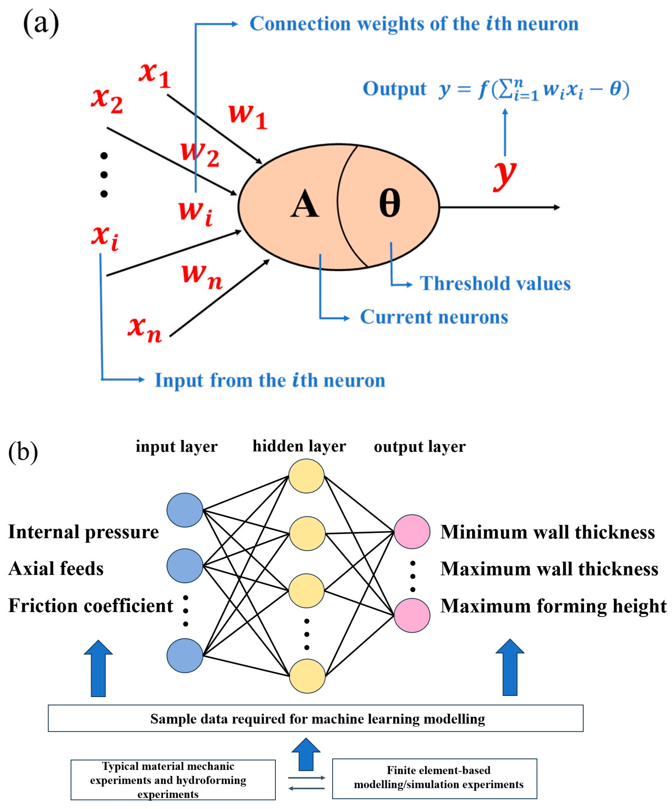
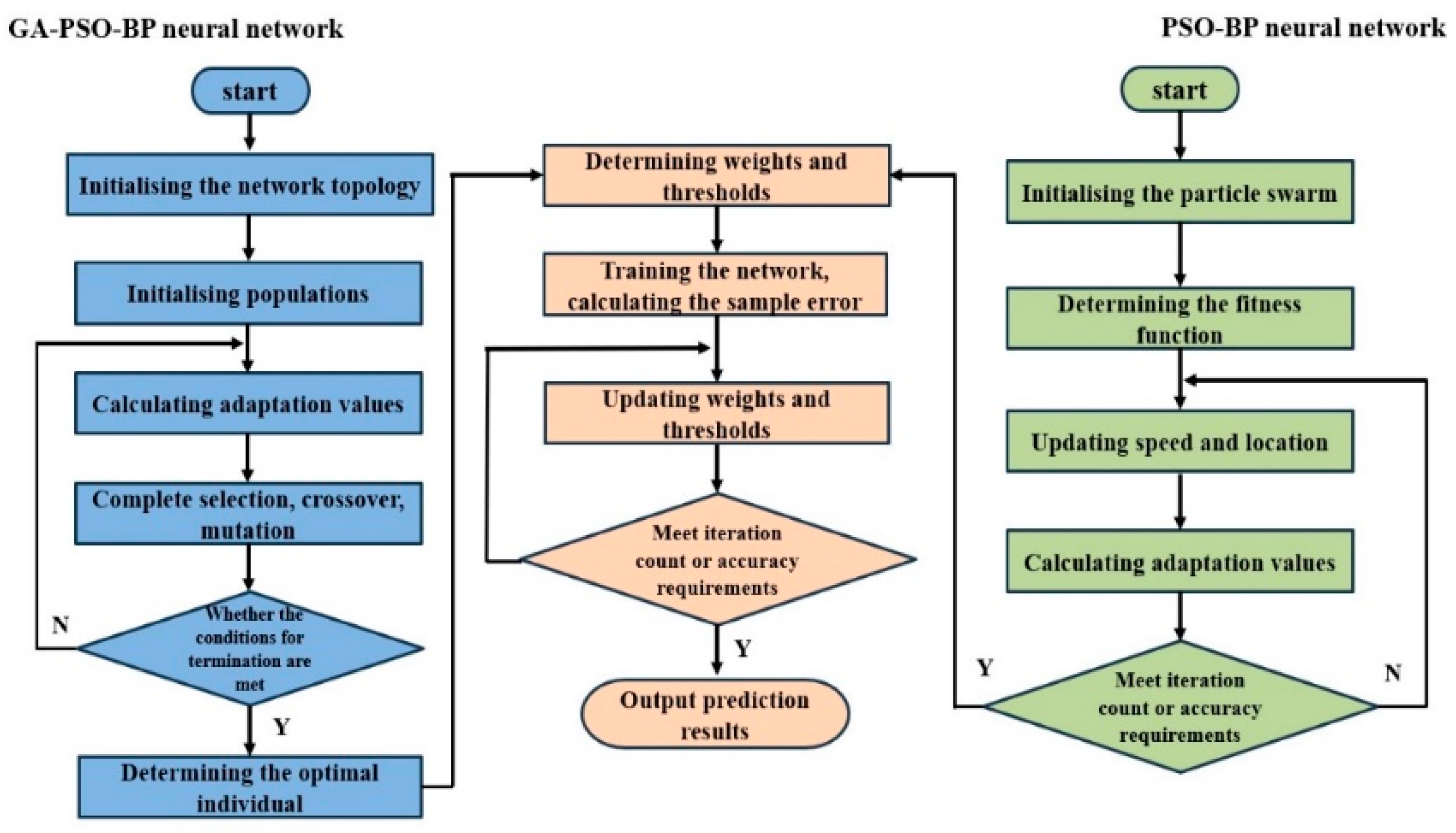
BP neural networks can approximate non-linear functions with arbitrary accuracy, but there are some drawbacks in use. In essence, the thresholds and weights are continuously adjusted by error back propagation and gradient descent, but, due to the cumbersome and slow error transfer process, the simulation results are unstable and prone to form local minima instead of global optimal solutions. There is also the problem that the selection of the number of hidden layer nodes and initial threshold weights is not supported by theoretical guidance. In this paper, two prediction models based on the particle swarm (PSO) optimisation of conventional BP neural network algorithms and the improvement of PSO-BP neural networks by introducing the hybridisation link in genetic algorithms (GA) are proposed for predicting the hydroforming effect.

4.1. Particle Swarm (PSO) Optimisation BP Neural Network Algorithm

Kennedy, James et al. proposed particle swarm optimisation (PSO) in 1995, which is a population algorithm for the intelligent optimisation of bionic class [14]. The basic idea is that a flock of birds does not know the exact location of the food, so the best way to find the food in the fastest possible way is to find the area of the flock that is closest to the food at the current location [15], finding optimal solutions through individual and group information sharing. The optimal weights are found by iterative optimisation of the particle swarm algorithm instead of the initialised weights in the traditional BP neural network. The basic parameters of the specific PSO-BP neural network model are shown in Table 6.

4.2. GA-PSO-BP Neural Network Model

This section details further introduction of hybridisation in genetic algorithms (GAs) based on the use of traditional BP neural networks optimised with particle swarms. The core idea of the GA is to simulate biological genetics and evolutionary theory to maintain the population towards optimal evolution, allowing populations to evolve through selection, crossover, and mutation operations to the emergence of optimal individuals [16]. This paper mainly studies the particle swarm optimisation algorithm as the main body to introduce the genetic operator of the genetic algorithm to achieve the improvement of the particle swarm algorithm, where the crossover operator is designed mainly by selecting the number of individuals in the new population after the action of the operator is assumed to be N. Take a randomised approach to forming [N/2] pairings, generating the two bodies produced by the crossover operation:
x 1 t + 1 = α x b t + 1 α x 1 t
x 2 t + 1 = α x 1 t + 1 α x b t
where α ∈ (0, 1) is the scaling factor, and the two parent individuals performing the crossover operation are x 1 t and x 2 t . x b t is the better adapted individual between the two parent individuals. The flow chart of the optimisation algorithm is shown in Figure 8.

4.3. GA-PSO-BP Model Accuracy Analysis

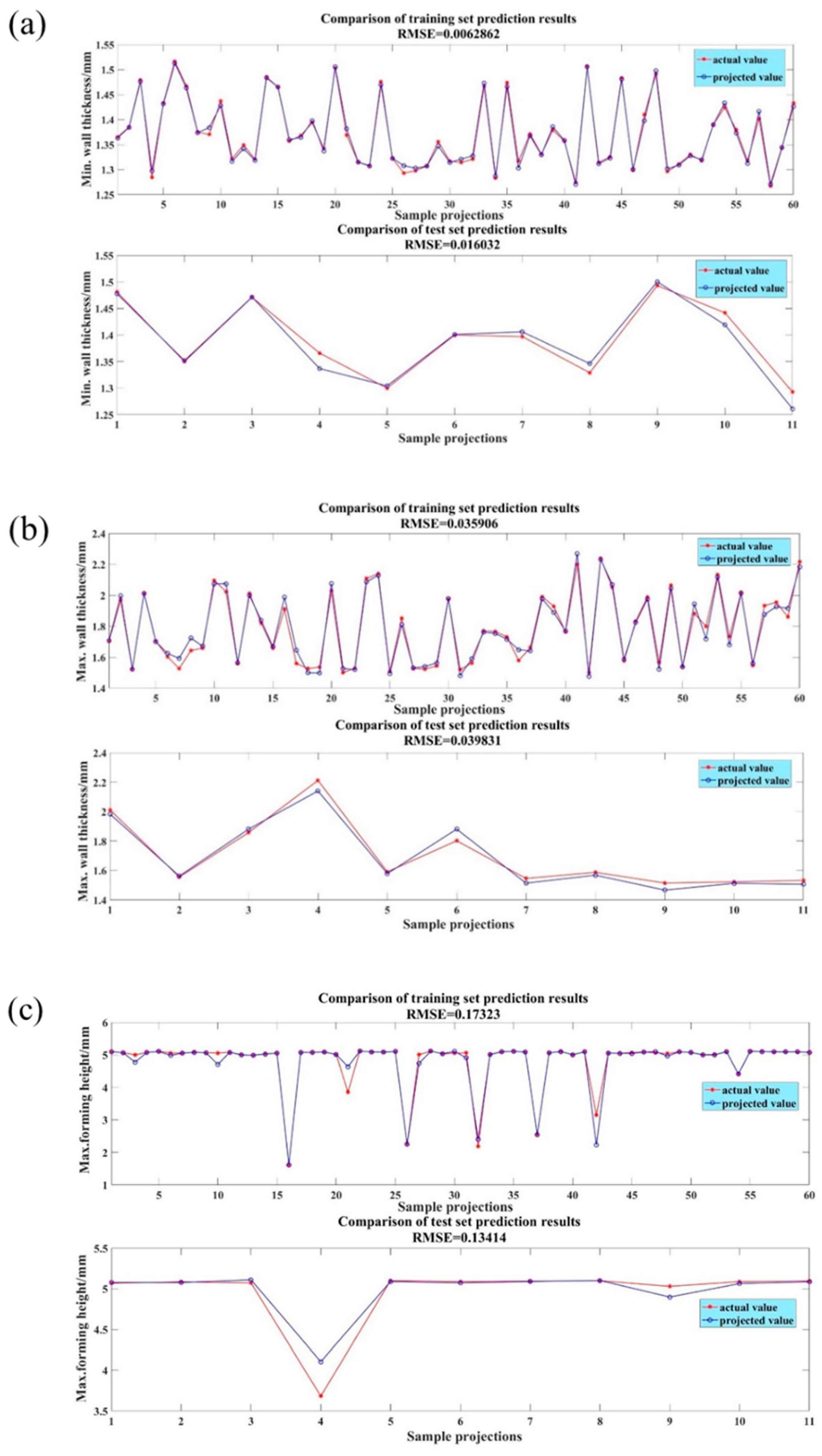
Comparison of the error results of the three prediction indexes (minimum wall thickness, maximum wall thickness, and maximum expansion height) based on the GA-PSO-BP neural network and the network performance evaluation results is shown in Figure 9 and Figure 10. Cross-validation was not utilised in the model construction for this research. The model accuracy was assessed through an evaluation of prediction errors across multiple forming quality metrics.
As shown in Figure 9 and 
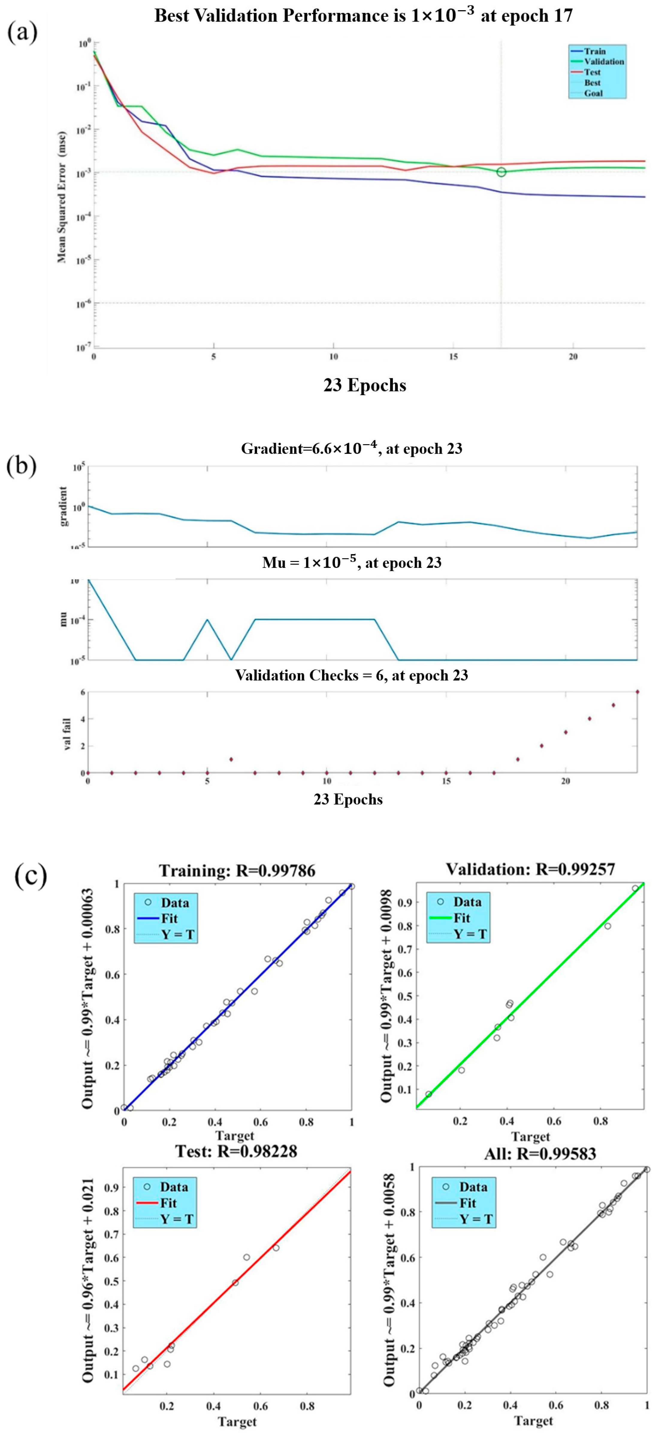
Figure 10, the optimisation error is very small: the BP neural network was stopped for a total of 20 iterations and reached the optimal validation result at the 17th iteration with an MSE of 0.0010366. These errors indicate the accuracy of the proposed method in determining the optimal solution. An accurate prediction of tube hydroforming parameters is provided by the THF model based on the GA-PSO-BP neural network, which provides an effective tool for optimising tube hydroforming process parameters in the shortest possible time. Figure 10c shows a plot of the predicted values of the neural network versus the actual values of the output patterns of the design matrix through the regression of training, validation, and test data. The coefficients of determination R 2 for the training and test sets are 0.99786 and 0.98228. The artificial neural network-based THF model provides accurate predictions of the aluminium alloy variable diameter tubes, forming parameters with 98% confidence level. Therefore, there is a good correlation between measured and predicted values. Based on neural network analysis, axial feeds and forming pressure have a greater effect on tube thinning and the accuracy of dimensions.

4.4. Comparison of BP, PSO-BP, and GA-PSO-BP Calculation Accuracy

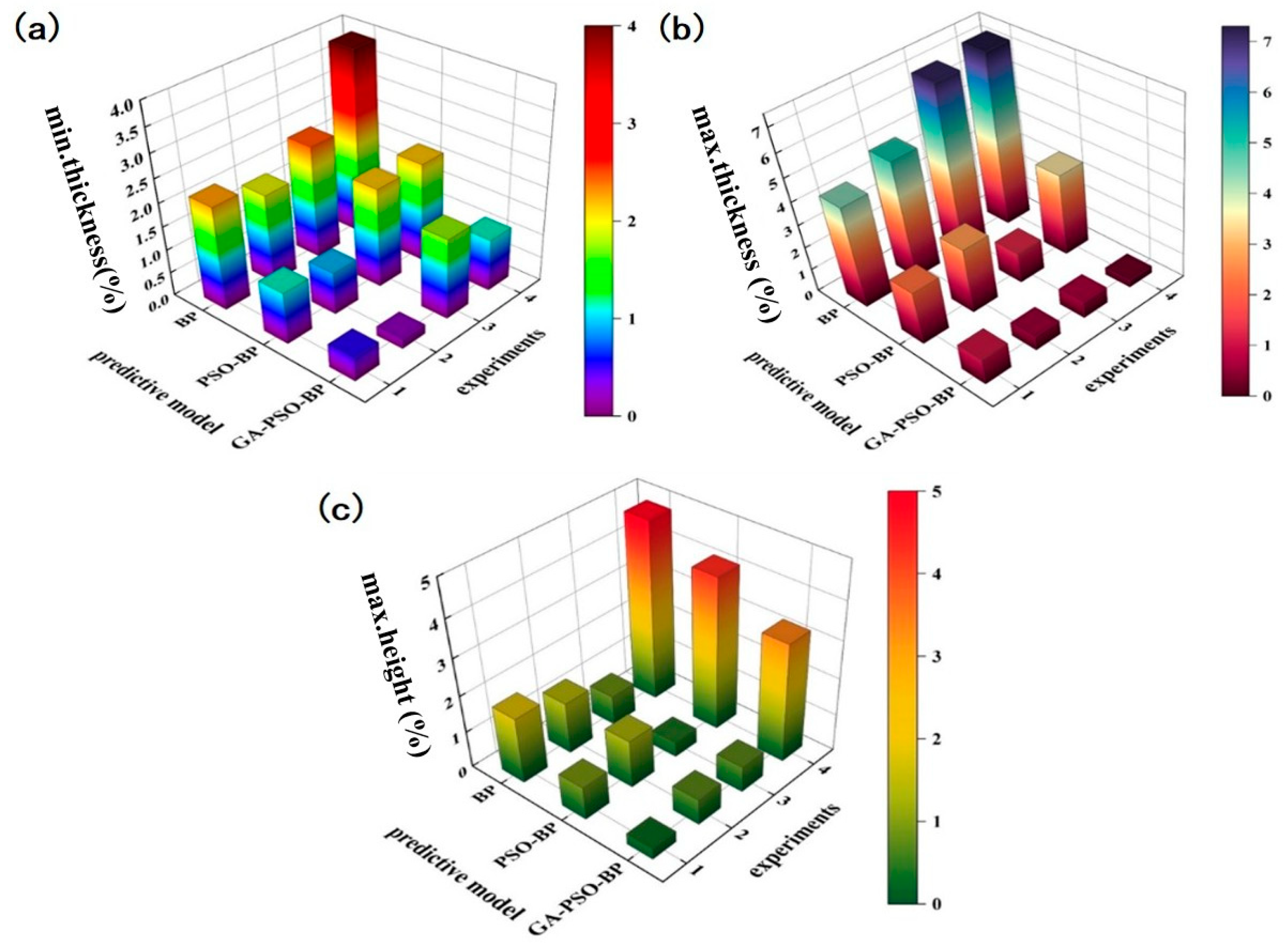
In order to further validate the prediction performance of the three machine learning prediction models, we combined these models with the simulation model of the EN AW 5052 aluminium alloy variable diameter tubes hydroforming constructed in the previous finite element simulation software. A comparison of the computational accuracy of models constructed based on BP neural networks and PSO-BP particle swarm optimisation neural network algorithms and models was based on genetically improved PSO-BP neural networks. The four sets of randomly selected data within the range of forming parameters need to be combined with the actual production experience of the aluminium alloy variable diameter tubes hydroforming and to avoid duplication with the database established in the previous section. The final set process parameters are shown in Table 7. The error analysis of the prediction and simulation results using the three models is shown in Figure 11.
Comparing the neural network prediction results and the finite element simulation results, it can be found that the neural network prediction model based on the GA-PSO-BP algorithm is in better agreement with the finite element simulation results. However, the second set of experiments shows from the input parameters and the forming effect that the condition is far from making the model reach the better-filled rate, and the deformation results of the tubes are not very informative. Therefore, the prediction result of the maximum expansion height of forming has a large error with the simulation result, and one of the reasons for the inaccurate prediction result is also related to the composition of the training set of the neural network model. In addition to this, the overall prediction accuracy is over 98%, which is a high prediction accuracy. It is fully demonstrated that the GA-PSO-BP neural network model for the prediction of hydraulic forming accuracy of the aluminium alloy variable diameter tubes established in this paper has good performance in the prediction of various parameters after forming, and it also verifies the reliability of the model in practical use.
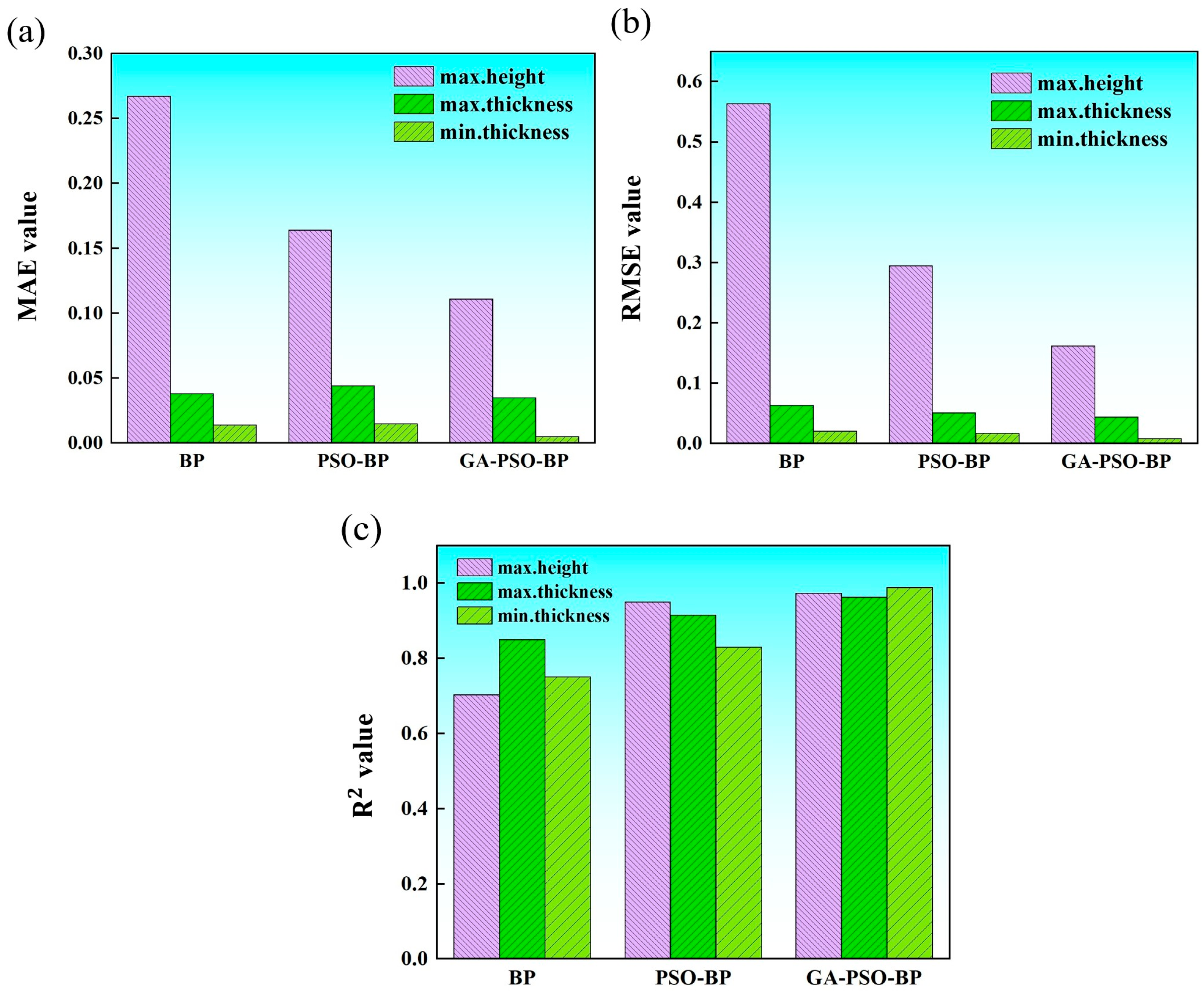
In order to more accurately judge the accuracy of the constructed model, in this paper, we will use the three performance metrics MAE, RMSE, and R 2 mentioned in the previous section to compare the performance of BP, PSO-BP, GA-PSO-BP models, respectively. The error comparisons of the three specific forming parameters using the three different algorithms are shown in Figure 12.
As can be seen from Figure 12, the neural network model established directly based on the BP algorithm, when forming results are predicted for the four groups of randomly selected data, the results for the minimum wall thickness and the maximum wall thickness forming parameters with respect to the R 2 evaluation indexes are 0.75 and 0.853, with a high prediction precision. However, the result for the maximum forming height with respect to the R 2 evaluation index is 0.703, which is still a large error. The introduction of the particle swarm optimisation algorithm is used to replace the initialised weights in the former by iterative optimisation search, so that the results of the three shaping parameter R 2 evaluation indexes of the improved model are 0.83, 0.915, and 0.950, and the prediction accuracy is effectively improved. However, the mean error function (MAE) is not greatly improved compared to the BP neural network. In order to balance the model’s ability to improve prediction accuracy while remaining as close as possible to the fitness obtained by fitting using the original test set, the hybridisation aspect of the genetic algorithm is introduced into the particle swarm iterative optimisation search process. Avoiding the phenomenon of the model falling into local search, it solves the problem that the model can easily fall into premature convergence and is unable to continue to iterate to seek the optimal solution when dealing with multi-dimensional problems, and it also achieves a balance between prediction accuracy and computational efficiency.
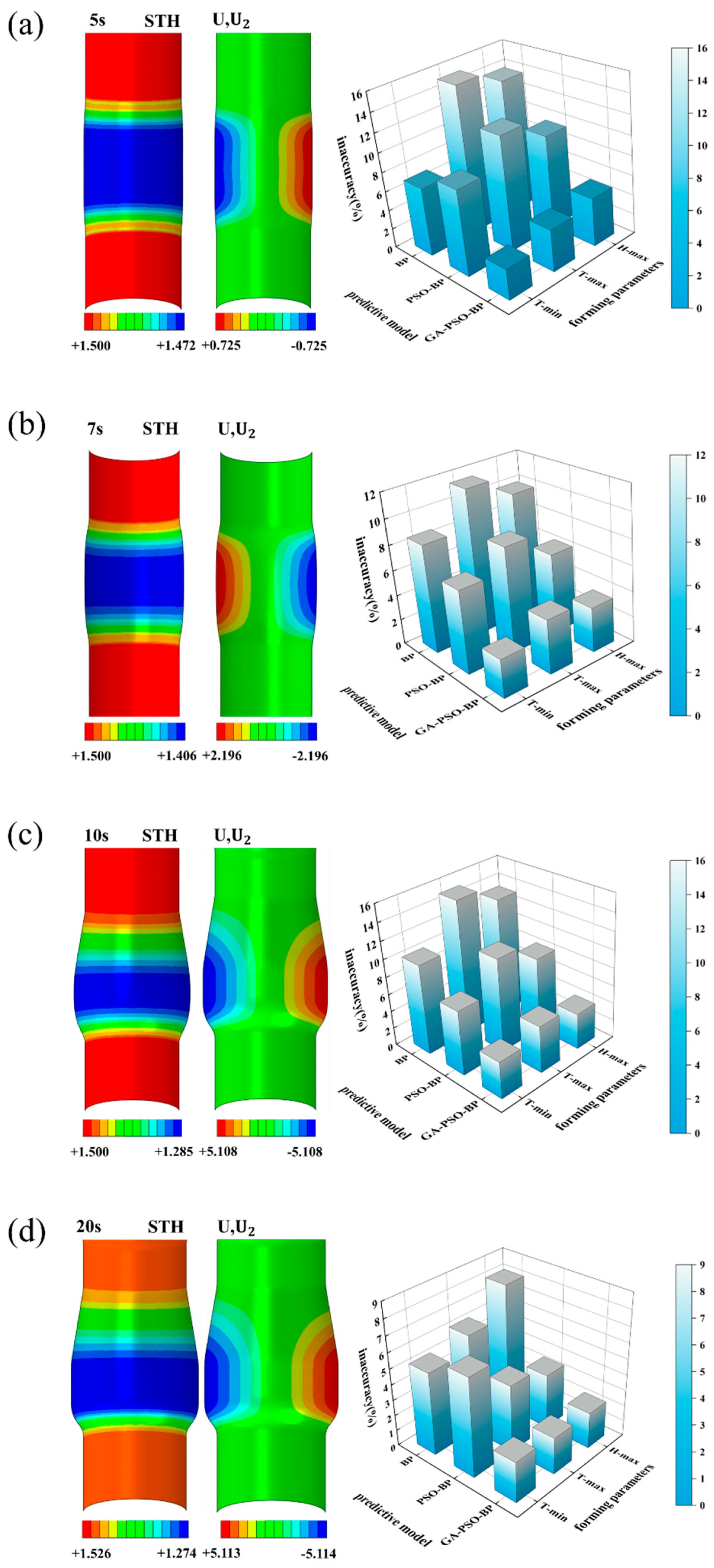
The process parameter combination for the hydroforming of aluminium alloy variable diameter tubes, which yielded the highest prediction accuracy, was determined using the GA-PSO-BP hybrid algorithm: The internal pressure is 40 MPa, the axial feed is 4 mm, and the friction coefficient is 0.15. After forming, the minimum wall thickness of the part is 1.27 mm, the maximum wall thickness is 1.53 mm, and the maximum height of forming is 5.11 mm. The finite element simulation results are shown in Figure 13.
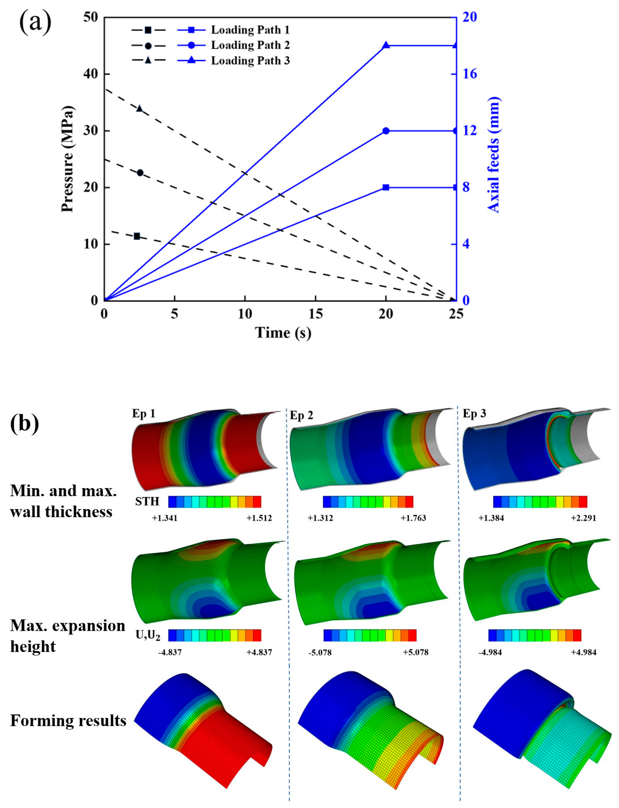
The specific forming process was divided into four stages of 5 s, 7 s, 10 s, and 20 s. The three neural network algorithms mentioned above were used to predict the three forming parameters, respectively, and, finally, the predicted values at different stages were compared with the simulated real values in terms of error. From the combined error comparison results, it was observed that the maximum expansion height parameter predictions exhibited larger errors across all three models. It was verified that the factors influencing expansion height were more complex during the initial hydroforming phase, when the tube first reached the state of plastic deformation, and before the tube reached the better-filled rate, as mentioned in the previous section. The influence of the aluminium large-section rate-of-change tube was included, which resulted in increased difficulty in achieving a linear relationship between the charge and internal pressure. Furthermore, the error comparison across different forming stages demonstrated that the forming parameter prediction errors of the GA-PSO-BP neural network model were maintained within ±4.5% for all stages.

4.5. Experimental Validation of Simulation Results

Hydroforming equipment and forming dies are shown in Figure 14. The equipment is 315 t special hydraulic moulding equipment, driven by servo motors. The forming die mainly consists of left and right push heads, upper and lower dies, and the experimental process uses tensile oil as a lubricant between the tube and the die [10].
Experimental testing of the simulation results used the previously mentioned machine learning forming parameters for aluminium alloy variable diameter tubes based on the GA-PSO-BP algorithm. The results were compared with the wall thickness and expansion height of the tube by selecting seven and five points at different locations on the outer contour of the axial profile of the tube. The results are shown in Figure 15, and the experimental and simulation results for the maximum thinning and thickening rates after tube forming are 15.3%, 3.3%, 14%, and 1.7%. The error between the experimental results and the simulation results is within ±5% with high accuracy, and the feasibility of combining finite element simulation on the intelligent control method of the aluminium alloy large section rate of change tube hydroforming was also verified.
Friction plays a crucial role in tube hydroforming [17]. Different coefficients of friction were achieved in the experiments through active lubrication or artificial roughness treatment. When the tube blank was left untreated, a coefficient of friction of approximately 0.12 was obtained. With active lubrication applied, the coefficient was reduced to about 0.05 [18], whereas artificial roughness treatment resulted in a coefficient of 0.2. Additionally, the coefficient of friction could be adjusted by varying both the type of lubrication employed and the degree of roughness introduced through artificial treatment.

5. Conclusions

In this paper, a fast prediction model based on the GA-PSO-BP neural network for the hydroforming of aluminium alloy variable diameter tubes was established. The main conclusions are as follows:
(1)
Compared with the PSO-BP prediction model and the traditional BP neural network prediction model, the GA-PSO-BP prediction model can control the coefficient of determination R 2 around 97% for the three forming parameters. The maximum mean absolute error (MAE) and mean square error (RMSE) are 0.111 and 0.162; the minimum mean absolute error (MAE) and mean square error (RMSE) are 0.005 and 0.008.
(2)
The optimum combination of process parameters is obtained after solving the following: the internal pressure is 40 MPa, the axial feed is 4 mm, and the friction coefficient is 0.15. After forming, the minimum wall thickness of the part is 1.27 mm, the maximum wall thickness is 1.53 mm, and the maximum height of expansion is 5.11 mm. The maximum thinning rate was 15.1 percent, and the maximum thickening rate was 1.8 percent. The end result is without visible defects and meets the criteria for tube hydroforming results.
(3)
The primary innovations of this study are focused on algorithmic advancements, along with the application of the proposed model to the field of plastic forming. The proposed methodology is not limited to hydroforming processes but can also be extended as a reference for other plastic-forming technologies such as tube bending and forging. Further research is required to determine optimal process parameters, such as through NSGA multi-objective optimisation algorithms, extension to rupture prediction, integration with real-time control, etc.

Author Contributions

Methodology, investigation, funding acquisition, conceptualisation supervision, Y.X.; software, investigation, validation, writing, X.Z.; methodology, investigation, conceptualisation, writing—reviewing and editing, W.X.; conceptualisation, writing—reviewing and editing, S.Z.; methodology, Y.T.; writing—reviewing and editing, L.C. All authors have read and agreed to the published version of the manuscript.

Funding

This research was financially supported by the National Natural Science Foundation of China [grant number 52405439] and the China Postdoctoral Science Foundation [grant number 2024M763339].The funder is Wenlong Xie.

Institutional Review Board Statement

Not applicable.

Informed Consent Statement

Not applicable.

Data Availability Statement

The raw data supporting the conclusions of this article will be made available by the authors on request.

Conflicts of Interest

The authors declare no conflicts of interest.

References

  1. Taub, A.; De Moor, E.; Luo, A.; Matlock, D.K.; Speer, J.G.; Vaidya, U. Materials for automotive lightweighting. Annu. Rev. Mater. Res. 2019, 49, 327–359. [Google Scholar] [CrossRef]
  2. Chu, G.; Sun, L.; Wang, G.; Fan, Z.; Li, H. Axial hydro-forging sequence for variable-diameter tube of 6063 aluminum alloy. J. Mech. Work. Technol. 2019, 272, 87–99. [Google Scholar] [CrossRef]
  3. Le, T.-K.; Bui, T.-A. Cold forging effect on the microstructure of motorbike shock absorbers fabricated by tube forming in a closed punch. Appl. Sci. 2021, 11, 2142. [Google Scholar] [CrossRef]
  4. Al-Bukhaiti, K.; Liu, Y.; Zhao, S.; Abas, H. An application of BP neural network to the prediction of compressive strength in circular concrete columns confined with CFRP. KSCE J. Civ. Eng. 2023, 27, 3006–3018. [Google Scholar] [CrossRef]
  5. Ray, P.; Mac Donald, B. Determination of the optimal load path for tube hydroforming processes using a fuzzy load control algorithm and finite element analysis. Finite Elements Anal. Des. 2004, 41, 173–192. [Google Scholar] [CrossRef]
  6. Ghorbani-Menghari, H.; Kahhal, P.; Jung, J.; Mohammadhosseinzadeh, M.; Moon, Y.H.; Kim, J.H. Multi-objective evolutionary neural network optimization of process parameters for double-stepped tube hydroforming. Int. J. Precis. Eng. Manuf. 2023, 24, 915–929. [Google Scholar] [CrossRef]
  7. Abbassi, F.; Ahmad, F.; Gulzar, S.; Belhadj, T.; Karrech, A.; Choi, H.S. Design of T-shaped tube hydroforming using finite element and artificial neural network modeling. J. Mech. Sci. Technol. 2020, 34, 1129–1138. [Google Scholar] [CrossRef]
  8. Chebbah, M.-S.; Lebaal, N. Tube hydroforming optimization using a surrogate modeling approach and Genetic Algorithm. Mech. Adv. Mater. Struct. 2020, 27, 515–524. [Google Scholar] [CrossRef]
  9. Xu, Y.; Zhang, X.; Xie, W.; Zhang, S.; Huang, X.; Tian, Y.; Chen, L. Fuzzy Control Optimization of Loading Paths for Hydroforming of Variable Diameter Tubes. Comput. Mater. Contin. 2024, 81, 2753–2768. [Google Scholar] [CrossRef]
  10. Liu, N.; Yang, H.; Li, H.; Tao, Z.; Hu, X. An imperfection-based perturbation method for plastic wrinkling prediction in tube bending under multi-die constraints. Int. J. Mech. Sci. 2015, 98, 178–194. [Google Scholar] [CrossRef]
  11. Der Kiureghian, A.; Liu, P. Structural reliability under incomplete probability information. J. Eng. Mech. 1986, 112, 85–104. [Google Scholar] [CrossRef]
  12. Liu, P.-L.; Der Kiureghian, A. Multivariate distribution models with prescribed marginals and covariances. Probabilistic Eng. Mech. 1986, 1, 105–112. [Google Scholar] [CrossRef]
  13. Feng, B.; Mao, J.; Hu, H. Springback Prediction Based on BP Neural Network for StripGigid Convex Characteristics. Forg. Technol. 2020, 45, 20–26. [Google Scholar]
  14. Kennedy, J.; Eberhart, R. Particle swarm optimization. In Proceedings of the ICNN’95—International Conference on Neural Networks, Perth, Australia, 27 November–1 December 1995; Volume 4. [Google Scholar] [CrossRef]
  15. Ekrem, Ö.; Aksoy, B. Trajectory planning for a 6-axis robotic arm with particle swarm optimization algorithm. Eng. Appl. Artif. Intell. 2023, 122, 106099. [Google Scholar] [CrossRef]
  16. Aivaliotis-Apostolopoulos, P.; Loukidis, D. Swarming genetic algorithm: A nested fully coupled hybrid of genetic algorithm and particle swarm optimization. PLoS ONE 2022, 17, e0275094. [Google Scholar] [CrossRef]
  17. Kasaei, M.M.; Naeini, H.M.; Abbaszadeh, B.; Hashemi, S.J.; da Silva, L.F. Improvement of material flow in tube hydroforming by advanced sealing methods. Proc. Inst. Mech. Eng. Part B J. Eng. Manuf. 2024, 238, 442–453. [Google Scholar] [CrossRef]
  18. Fan, Y.; Xu, X.; Wang, L.; Zhang, J. Differential lubrication optimization of T-tube hydroforming. J. Plast. Eng. 2022, 29, 44–52. [Google Scholar]
Figure 1. (a) Principle of tube hydroforming, (b) size of target part.
Applsci 15 05045 g001
Figure 2. Stress–strain curve of EN AW 5052: (a) engineering, (b) true.
Applsci 15 05045 g002
Figure 3. (a) Finite element model. (b) Mesh fitness analysis.
Applsci 15 05045 g003
Figure 4. Schematic diagram of filling rate of corners.
Applsci 15 05045 g004
Figure 5. (a) Loading path curve. (b) Finite element forming results.
Applsci 15 05045 g005
Figure 6. Sample distribution in 3D.
Applsci 15 05045 g006
Figure 7. (a) M-P neuron model. (b) Machine learning-based modelling of the large section rate of change tube hydroforming process control.
Applsci 15 05045 g007
Figure 8. Flow chart of GA-PSO-BP algorithm.
Applsci 15 05045 g008
Figure 9. Comparison of RMSE results between training set and test set: (a) min. wall thickness, (b) max. wall thickness, (c) max. forming thickness.
Applsci 15 05045 g009
Figure 10. (a) Performance of training process network, (b) optimal iteration results, (c) distribution of forecast results and coefficient of determination R 2 .
Applsci 15 05045 g010
Figure 11. Comparison of error between prediction and simulation results: (a) Min. wall thickness. (b) Max. wall thickness. (c) Max. forming height.
Applsci 15 05045 g011
Figure 12. Comparison of the prediction errors of different prediction models for the forming parameters: (a) MAE, (b) RMSE, (c) R 2 .
Applsci 15 05045 g012
Figure 13. Error plots of finite element results of the forming process versus model predictions: (a) 5 s, (b) 7 s, (c) 10 s, (d) 20 s.
Applsci 15 05045 g013
Figure 14. Servo hydroforming equipment and dies.
Applsci 15 05045 g014
Figure 15. Comparison of simulated and experimental results: (a) Thickness distribution. (b) Distension height distribution.
Applsci 15 05045 g015
Table 1. Mechanical properties of EN AW 5052.
ParametersDensitiesElastic ModulusPoisson’s RatioYield StrengthTensile StrengthElongation
Values2.68 g/cm370 GPa0.3395 MPa203 MPa20%
Table 2. Sample data for some process parameters.
No. Process Parameters
Internal Pressure (MPa)Axial Feeds (mm)Friction Coefficient
15016.310.07
27.3110.560.1
339.6215.490.03
457.690.15
539.628.10.025
614.239.740.05
710.774.820.05
836.1514.670.1
943.0811.790.18
1037.3119.590.06
1117.6910.150.2
1223.466.050.08
Table 3. Corresponding mean square error for different number of neuron nodes in hidden l.
Number of Hidden Layer NodesMSE 1MSE 2MSE 3MSE
30.0007290.00640.1513210.151321
40.000251860.003317760.098200760.09820076
50.000419060.061388550.169101890.16910189
60.000260340.00448190.258206260.25820626
70.000168820.002122440.205852760.20585276
80.000365230.002328160.230851420.23085142
90.000431190.004588170.045198760.04519876
100.000392280.005706440.123763240.12376324
110.000136050.002533910.098044130.09804413
120.000256480.004997360.13665340.1366534
Table 4. Basic parameters of BP neural network.
ParametersValueInstruction
Network topology3-9-3——
Number of iterations1000——
Error thresholds 1 × 10 6 ——
Learning rate0.01——
h-o activation functiontan-sigmoidHyperbolic tangent S-functions
o activation functionpurelinLinear function
Training algorithmtrainlmLevenberg–Marquardt, L-M
Table 5. BP neural network prediction performance test.
Output Layer FactorsMAERMSE R 2
Min. wall thickness0.0390.0470.827
Max. wall thickness0.0550.0880.867
Max. forming height0.4820.6720.748
Table 6. PSO-BP neural network prediction performance test.
ParametersValueParametersValue
Training samples59Input nodes3
Test samples11Hidden layer nodes7
Learning rate0.01Output nodes3
Training steps1000Stock size5
Training functiontrainlmStock iterations30
Hidden layer excitation functiontan-sigmoidLearning factor c 1 4.494
Output layer excitation functionpurelinLearning factor c 2 4.494
Table 7. Validation of experimental process parameters.
No.Internal Pressure/MPaAxial Feeds/mmFriction Coefficient
136.410.80.1
2308.680.15
312.583.430.2
424.667.680.05
Disclaimer/Publisher’s Note: The statements, opinions and data contained in all publications are solely those of the individual author(s) and contributor(s) and not of MDPI and/or the editor(s). MDPI and/or the editor(s) disclaim responsibility for any injury to people or property resulting from any ideas, methods, instructions or products referred to in the content.

