Design of Parameter Adaptive Suspension Controllers with Kalman Filter for Ride Comfort Enhancement and Motion Sickness Reduction

Featured Application

Parameter adaptive controller design for ride comfort improvement and motion sickness reduction in electric vehicles with autonomous driving function.

Abstract

This paper presents a method to design a parameter adaptive suspension controller to boost ride comfort and to reduce motion sickness. According to recently published papers, combined motions of a sprung mass (SPMS) along heave and pitch directions tend to make motion sickness severe. To reduce motion sickness, it is necessary to design a controller which can reduce the heave and pitch vibrations of a SPMS. To avoid full-state feedback which is very difficult to implement in a real vehicle, a static output feedback (SOF) control is chosen as a feedback structure. With the SOF structure, linear quadratic SOF and parameter adaptive controllers are designed. When designing parameter adaptive controllers, an extended Kalman filter (EKF), equivalent to recursive least square (RLS), is selected for parameter adaptation. To verify performance of the controllers, simulation is performed on vehicle simulation tool. From simulation responses, it is checked whether the proposed parameter adaptive controllers are effective or not and which is the best controller, with respect to ride comfort and motion sickness.

1. Introduction

Up to date, it has been widely known that there are two key objectives when designing a suspension controller: vibration isolation and road holding, related to occupant’s ride comfort (RC) and vehicle handling/agility/safety, respectively [1,2,3]. Generally, the ride comfort and handling are quantified with heave acceleration (a_zc) of a sprung mass (SPMS) and tire deflection, correspondingly [1]. Most studies in the area of suspension control have tried to improve RC by reducing a_zc with a controller [3,4,5].

For the last decade, motion sickness (MS) has been taken into account as a new objective in the area of suspension control due to the recent rapid spread of electric vehicles (EVs) and autonomous driving. In case of EVs, high output torque of an electric motor and regenerative braking, needed to charge battery, can cause abrupt change in the longitudinal acceleration and its consequent pitch rate (ω_yc) of a SPMS. This can result in severe motion sickness [6,7,8]. In case of autonomous driving, it has been predicted that autonomous driving function can convert passenger’s driving tasks to non-driving ones [9,10,11,12,13]. However, this benefit may result in visual-vestibular conflict, which has been regarded as a main source of MS [9,10,11,12,13,14]. To cope with this problem in vehicles with autonomous driving functions, various methods have been applied to date [15,16]. Among them, one method is to design a suspension controller to reduce MS [17,18,19,20].

Figure 1 shows the frequency weightings specified in ISO2631-1, a standard that evaluates how the human body is affected by whole-body vibration [19,21,22]. In Figure 1, the weights W_k:V and W_f:MS represent a_zc, a measure of RC and MS, over the frequency ranges from 4.0 to 10.0 Hz and from 0.1 to 0.2 Hz, correspondingly. On the other hand, it was reported that MS worsened by combined stimulation, (a_zc,ω_yc), over the frequency range from 0.8 to 8.0 Hz. The weight W_f:Dizio in Figure 1 represents this fact [23,24]. Different from W_k:V and W_f:MS, W_f:Dizio is overlapped with W_k:V over the frequency range from 4.0 to 10.0 Hz. For this reason, RC can be improved, and MS can be reduced if a suspension controller can reduce a_zc and ω_yc over the frequency range from 0.8 to 8.0 Hz. Based on this fact, the purpose of this paper is to design a suspension controller for RC enhancement and MS reduction. For the purpose, the previous works adopted a static output feedback (SOF) control method and applied it to reduce a_zc and ω_yc with an active suspension [17,18,19,20].

Several controller design methodologies have been proposed to suspension control up to date [3,4,5]. Among them, linear quadratic optimal control (LQOC), including LQR, is the most well-known methodology because of its relative importance among several objectives such as RC, MS, handling and rollover prevention, which is easy to exquisitely tune with LQR [5]. When designing LQR as suspension controller design, it needs a state-space equation (SSEQN) and LQ objective function (LQOF). To describe the heave and pitch motions of a SPMS, a half-car model (HCM) is selected as a vehicle one. From the model, a linear SSEQN is derived. In this paper, an active suspension is selected as an actuator, used to generate vertical control forces with limited bandwidth [17,18,19,20].

Generally, LQR adopts full-state feedback (FSF), which needs all states in a state vector to be measured or estimated. However, it is very difficult and very expensive to measure or estimate total states with sensors in real vehicles. In addition, LQR has plenty of gain elements, which makes it harder to implement LQR on real vehicles. To deal with the problem, a SOF control has been selected because it uses only available sensor outputs in real vehicles, and it has a smaller number of gain elements [25,26,27,28,29,30,31]. Especially, the previous works have used only two sensor signals for the HCM [17,18,19,20]. For that reason, SOF is selected as a feedback structure in this paper. Especially, two types of SOF structure are proposed.

For each SOF structure, two pairs of sensor outputs are proposed for SOF control. The first pair is the vertical velocity(v_zc) and ω_yc, and the second is the suspension stroke and its rate or the suspension displacement and suspension velocity. Those signals are measured at the front and rear suspensions. HCM has two control inputs in the front and rear suspensions. Accordingly, the SOF controllers (SOFCs) have gain matrices of 2 × 4 and 2 × 2 dimensions for the first and second pairs of sensor outputs, respectively. Those SOFCs are optimized with LQOF. To find optimal gain matrices of SOFCs in this paper, a meta-heuristic method is applied [32,33]. The SOFCs with optimal gain matrices are called LQ SOF controllers (LQSOFCs).

In addition to feedback, the other issues in the area of suspension control are robustness, ability to guarantee control performance under parameter uncertainty and nonlinearity in a plant, disturbance attenuation, and ability to reduce the effects of external disturbance on control performance. In suspension control, external disturbances have much more effects on control performance than parameter uncertainty and nonlinearity. To cope with the problem, several robust controller design methodologies such as LQ optimal control, H₂/H_∞ control, robust model predictive control, adaptive control has been applied to vehicle suspension control to date [1,4,5]. Among them, an adaptive control is selected in this paper because it can adaptively change a controller according to parameter uncertainty and nonlinearity in a plant and can effectively attenuate the effects of external disturbances [34,35,36,37,38]. In this paper, adaptive control means that the gains of SOFC are adaptively updated by a parameter adaptation algorithm. Let denote this controller as parameter adaptive controller (PAC). While LQSOFC has the constant gain matrix, PAC adaptively updates the gains in every step by a parameter adaptation algorithm [34,35,36,37,38]. In other words, PAC is a learning-based controller, which tries to minimize an error by a learning mechanism [36]. To date, a recursive least square (RLS) has been well-known as a parameter adaptation algorithm. In addition, it was shown that RLS is equivalent to Kalman filter [39]. The unique feature of the Kalman filter is that it can be used for both state and parameter estimation. Using this feature, the dual extended Kalman filter (DEKF) has been applied to vehicle control [40,41,42,43,44,45]. For that reason, the extended Kalman filter (EKF) is selected for parameter adaptation in this paper because EKF can easily handle multiple outputs [40,41,42,43,44,45]. Contrastingly to LQSOFC with constant gains, PAC can cope with parameter uncertainties, nonlinearities and external disturbances by using parameter adaptation with EKF [38].

To verify the performance of LQSOFCs and PACs, a simulation is performed on a vehicle simulation software. Based on simulation responses, the effect of PAC in respect of RC and MS is shown.

The objective of this paper is to design LQSOFCs and PACs based on SOF structure for RC enhancement and MS reduction. The contributions of this paper can be summarized as follows:

• Two types of SOFCs are proposed and designed to reduce a_zc and ω_yc over the frequency range from 0.8 to 8.0 Hz. Those SOFCs are optimized with LQOF and validated through simulation on a vehicle simulation package.
• PACs are proposed with two SOF structures and EKF. Differently from LQSOFCs, PAC can adaptively update gains of SOFCs under parameter uncertainties, nonlinearities and external disturbances.
• With LQSOFCs and PACs, the simulation is performed on CarSim. From simulation responses, it is identified which controller can give the best performance in relation to RC and MS.

This paper is composed of five sections. A HCM is presented and its linear SSEQN is derived in Section 2. With the linear SSEQN, two SOFCs are proposed and optimized with LQOF. PAC is designed in Section 3. In Section 4, a simulation with LQSOFCs and PACs is performed and the simulation responses are analyzed and discussed. The conclusions are presented in Section 5.

2. Design of LQ Optimal Controllers

2.1. Half-Car Model and Derivation of State-Space Equation

When designing LQ optimal controllers such as LQR and LQSOFC, a linear SSEQN is needed. Generally, a linear SSEQN is derived from a linear vehicle model. To describe the heave and pitch motions of a SPMS and the vertical motions of unsprung masses (USPMSs), a HCM is selected as a vehicle one in this paper [17,19,20]. Figure 2 shows the HCM with linear springs and dampers and its parameters and variables. In Figure 2, S_f and S_r stand for the front and rear suspensions, respectively. u_f and u_r are the control input or the vertical control force generated by an active actuator in S_f and S_r. The parameters in the HCM are described in Nomenclature. Let denote the front and rear corners of the SPMS as FC_SPMS and RC_SPMS, respectively. In Figure 2, z_sf and z_sr are the vertical displacements of FC_SPMS and RC_SPMS, respectively.

In Figure 2, the suspension displacements, suspension velocities and tire deflections of S_f and S_r are defined as (1), where d, v and w stand for the suspension displacement, the suspension velocity and the tire deflection, respectively. With those definitions, the suspension forces at S_f and S_r are derived as (2). As shown in (2), the suspension forces are calculated with d and v at S_f and S_r. With (2), the equations of heave and pitch motions of the SPMS, m_s and the vertical motions of USPMSs, m_uf and m_ur, are obtained as (3). From the spatial relationship between the center of gravity (C.G.) and FC_SPMS/RC_SPMS, and the approximation, sinθ_c ≈ θ_c, z_sf and z_sr, the vertical displacements at FC_SPMS and RC_SPMS, are obtained as (4) from z_c and θ_c. The value of (4) is converted into the matrix-vector form of (5). New vectors and matrices are defined as (6), where x, w and u are the vectors of state variables, disturbances and control inputs, respectively. With these definitions in (6), the suspension force of (2) is represented by (7). With (6) and (7), the equation of the sprung mass given in (3) is converted into (8), and the vertical displacements of (5) are converted into (9). With (7) and (9), (8) is converted into (10). A new matrix-vector Equation (11) is derived from (10). With the new matrices defined in (11) and the vector z defined in (6), (12) is obtained. By defining new matrices A, B₁ and B₂ as given in (13), the SSEQN of the HCM is obtained as (14).

$$\left\{\begin{array}{c}{d}_f\triangleq z_{sf}-z_{uf}\\ d_r\triangleq z_{sr}-z_{ur}\end{array}\right.\hspace{1em}\left\{\begin{array}{l}{v}_f\triangleq {\dot{z}}_{sf}-{\dot{z}}_{uf}\\ v_r\triangleq {\dot{z}}_{sr}-{\dot{z}}_{ur}\end{array}\right.\hspace{1em}\left\{\begin{array}{c}{w}_f\triangleq z_{uf}-z_{rf}\\ w_r\triangleq z_{ur}-z_{rr}\end{array}\right.\hspace{1em},$$

(1)

$$\left\{\begin{array}{l}{f}_f=-k_{sf}\left(z_{sf}-z_{uf}\right)-b_{sf}\left({\dot{z}}_{sf}-{\dot{z}}_{uf}\right)+u_f=-k_{sf}{d}_f-b_{sf}{v}_f+u_f\\ f_r=-k_{sr}\left(z_{sr}-z_{ur}\right)-b_{sr}\left({\dot{z}}_{sr}-{\dot{z}}_{ur}\right)+u_r=-k_{sr}{d}_r-b_{sr}{v}_r+u_r\end{array}\right.,$$

(2)

$$\left\{\begin{array}{l}{m}_s{\ddot{z}}_c=f_f+f_r\hfill \\ I_y{\ddot{\theta }}_c=-l_f{f}_f+l_r{f}_r\hfill \end{array}\right.\hspace{1em}\hspace{1em}\left\{\begin{array}{l}{m}_{uf}{\ddot{z}}_{uf}=-f_f-k_{tf}{w}_f\hfill \\ m_{ur}{\ddot{z}}_{ur}=-f_r-k_{tr}{w}_r\hfill \end{array}\right.,$$

(3)

$$\left\{\begin{array}{c}{z}_{sf}=z_c-l_f\sin {\theta }_c\simeq z_c-l_f{\theta }_c\\ z_{sr}=z_c+l_r\sin {\theta }_c\simeq z_c+l_r{\theta }_c\end{array}\right.,$$

(4)

$$\left[\begin{array}{c}{z}_{sf}\\ z_{sr}\end{array}\right]=\left[\begin{array}{cc}1& -l_f\\ 1& l_r\end{array}\right]\left[\begin{array}{c}{z}_c\\ {\theta }_c\end{array}\right],$$

(5)

$$\begin{array}{c}p\triangleq \left[\begin{array}{c}{z}_c\\ {\theta }_c\end{array}\right],\hspace{0.33em}{z}_s\triangleq \left[\begin{array}{c}{z}_{sf}\\ z_{sr}\end{array}\right],\hspace{0.33em}{z}_u\triangleq \left[\begin{array}{c}{z}_{uf}\\ z_{ur}\end{array}\right],\hspace{0.33em}{z}_r\triangleq \left[\begin{array}{c}{z}_{rf}\\ z_{ru}\end{array}\right],\hspace{0.33em}z\triangleq \left[\begin{array}{c}p\\ z_u\end{array}\right],\hspace{0.33em}f\triangleq \left[\begin{array}{c}{f}_f\\ f_r\end{array}\right],\hspace{0.33em}G\triangleq \left[\begin{array}{cc}1& 1\\ -l_f& l_r\end{array}\right]\\ x\triangleq \left[\begin{array}{c}z\\ \dot{z}\end{array}\right]\hspace{0.33em},\hspace{0.33em}w\triangleq z_r\hspace{0.33em},\hspace{0.33em}u\triangleq \left[\begin{array}{c}{u}_f\\ u_r\end{array}\right]\\ M_s\equiv \mathrm{diag}\left(m_s,I_y\right),\hspace{0.33em}{M}_u\equiv \mathrm{diag}\left(m_{uf},m_{ur}\right)\\ K_s\equiv \mathrm{diag}\left(k_{sf},k_{sr}\right),\hspace{0.33em}{B}_s\equiv \mathrm{diag}\left(b_{sf},b_{sr}\right),\hspace{0.33em}{K}_t\equiv \mathrm{diag}\left(k_{tf},k_{tr}\right)\end{array},$$

(6)

$$f=-K_s\left(z_s-z_u\right)-B_s\left({\dot{z}}_s-{\dot{z}}_u\right)+u,$$

(7)

$$\left\{\begin{array}{l}{M}_s\ddot{p}=Gf\hspace{1em}\Rightarrow \hspace{1em}\left[\begin{array}{c}{m}_s{\ddot{z}}_c\\ I_y{\ddot{\theta }}_c\end{array}\right]=\left[\begin{array}{cc}1& 1\\ -l_f& l_r\end{array}\right]\left[\begin{array}{c}{f}_f\\ f_r\end{array}\right]=Gf\\ M_u{\ddot{z}}_u=-f-K_t\left(z_u-z_r\right)\end{array}\right.,$$

(8)

$$z_s=G^{T}p\hspace{1em}\iff \hspace{1em}p={\left(G^T\right)}^{-1}{z}_s,$$

(9)

$$\left\{\begin{array}{l}{M}_s\ddot{p}=-G{K}_s\left(G^{T}p-z_u\right)-G{B}_s\left(G^T\dot{p}-{\dot{z}}_u\right)+Gu\\ M_u{\ddot{z}}_u=K_s\left(G^{T}p-z_u\right)+B_s\left(G^T\dot{p}-{\dot{z}}_u\right)-u-K_t\left(z_u-z_r\right)\end{array}\right.,$$

(10)

$$\underset{M}{\underbrace{\left[\begin{array}{cc}{M}_s& 0_{2\times 2}\\ 0_{2\times 2}& M_u\end{array}\right]}}\left[\begin{array}{c}\ddot{p}\\ {\ddot{z}}_u\end{array}\right]=\underset{K}{\underbrace{\left[\begin{array}{cc}-G{K}_s{G}^T& G{K}_s\\ K_s{G}^T& -K_s-K_t\end{array}\right]}}\left[\begin{array}{c}p\\ z_u\end{array}\right]+\underset{B}{\underbrace{\left[\begin{array}{cc}-G{B}_s{G}^T& G{B}_s\\ B_s{G}^T& -B_s\end{array}\right]}}\left[\begin{array}{c}\dot{p}\\ {\dot{z}}_u\end{array}\right]+\underset{U}{\underbrace{\left[\begin{array}{c}G\\ -I_{2\times 2}\end{array}\right]}}u+\underset{L}{\underbrace{\left[\begin{array}{c}{0}_{2\times 2}\\ K_t\end{array}\right]}}{z}_r,$$

(11)

$$M\ddot{z}=K\dot{z}+Bz+Uu+Lw,$$

(12)

$$A\equiv \left[\begin{array}{cc}{0}_{4\times 4}& I_{4\times 4}\\ M^{-1}K& M^{-1}B\end{array}\right],\hspace{0.33em}{B}_1\equiv \left[\begin{array}{c}{0}_{4\times 2}\\ M^{-1}L\end{array}\right],\hspace{0.33em}{B}_2\equiv \left[\begin{array}{c}{0}_{4\times 2}\\ M^{-1}U\end{array}\right],$$

(13)

$$\dot{x}=Ax+B_{1}w+B_{2}u.$$

(14)

2.2. Design of LQR

The LQ objective function (LQOF), L, is defined as (15). In the LQOF, control objectives can be tuned by setting the weight, ρ _i, higher or lower while maintaining the others fixed. In (15), the weight ρ _i in L is tuned by Bryson’s rule, (16), where ξ_i is the maximum allowable value (MAV) on i-th term in L [17,18,19,20,46]. For RC, ξ₁ on a_zc should be set as small as possible. For MS reduction, ξ₁ on a_zc and ξ₃ on ω_yc should be set as small as possible. For road holding, ξ₅ on (d_f, d_r) and ξ₆ on (w_f, w_r) should be set as small as possible. With the matrices A, B₂, Π, Ξ and Θ given in (14) and (15), the control input of LQR is computed as the FSF form of (17).

$$\begin{array}{l}L={\displaystyle {\int }_0^{\infty }\left\{{\rho }_1{\ddot{z}}_c^2+{\rho }_2{\ddot{\theta }}_c^2+{\rho }_3{\dot{\theta }}_c^2+{\rho }_4{\theta }_c^2+{\rho }_5{\displaystyle \sum _{i=f,r}{d}_i^2}+{\rho }_6{\displaystyle \sum _{i=f,r}{w}_i^2}+{\rho }_7{\displaystyle \sum _{i=f,r}{u}_i^2}\right\}dt}\hspace{1em}\\ \hspace{0.33em}\hspace{0.33em}={\displaystyle {\int }_0^{\infty }\left\{{\left[\begin{array}{c}x\\ u\end{array}\right]}^T\left[\begin{array}{cc}\Pi & \Xi \\ {\Xi }^T& \Theta \end{array}\right]\left[\begin{array}{c}x\\ u\end{array}\right]\right\}dt},\hspace{1em}\end{array}$$

(15)

$${\rho }_i={\displaystyle \frac{1}{{\xi }_i^2}},\hspace{1em}i=1,2,\cdots ,7,$$

(16)

$$u=-K_{LQR}x=-{\Theta }^{-1}{B}_2^{T}Px.$$

(17)

2.3. Design of LQ SOF Controllers

Generally, we know that all state variables of x are difficult or very expensive to measure with sensors in a real vehicle. Moreover, LQR has plenty of gain elements, which are hard to implement in a real vehicle. To resolve those problems, a SOF control has been adopted as feedback structure so far [17,18,19,20,29,30]. Unlike the FSF, a SOFC uses available sensor signals in a real vehicle.

In this paper, two vectors of available sensor outputs, y₁ and y₂, are derived from the state vector x as (18) and (19), respectively. In (18), y₁ represent the suspension displacements, d_f and d_r, and the suspension velocities, v_f and v_r, of S_f and S_r, correspondingly [25,29,30]. As shown in (19), the available outputs of y₂ are v_zc and ω_yc [17,18,20].

$$y_1\triangleq \left[\begin{array}{c}{d}_f\\ v_f\\ d_r\\ v_r\end{array}\right]=C_{1}x=\left[\begin{array}{cccccccc}1& -l_f& -1& 0& 0& 0& 0& 0\\ 0& 0& 0& 0& 1& -l_f& -1& 0\\ 1& l_r& 0& -1& 0& 0& 0& 0\\ 0& 0& 0& 0& 1& l_r& 0& -1\end{array}\right]x,$$

(18)

$$y_2\triangleq \left[\begin{array}{c}{\dot{z}}_c\\ {\dot{\theta }}_c\end{array}\right]=\left[\begin{array}{c}{v}_{zc}\\ {\omega }_{yc}\end{array}\right]=C_{2}x=\left[\begin{array}{cccccccc}0& 0& 0& 0& 1& 0& 0& 0\\ 0& 0& 0& 0& 0& 1& 0& 0\end{array}\right]x.$$

(19)

With y₁, the first SOFC, u_SOF1, is proposed as (20) [29,30]. This is similar to the suspension forces, f_f and f_r, as shown in (2). In other words, four gains, k_f1, k_f2, k_r1 and k_r2 of (20) correspond to k_sf, b_sf, k_sr and b_sr of (2), respectively. The first SOFC, u_SOF1, reflects the fact that the control inputs, u_f and u_r, are determined by S_f and S_r, respectively. This assumes that the vertical motions of FC_SPMS and RC_SPMS are independent K_SOF1. As shown in (20), K_SOF1 is structured. In other words, K_SOF1 does not have full elements. This makes an optimization procedure difficult when finding K_SOF1 minimizing L.

$$u_{SOF1}=K_{SOF1}{y}_1=\left[\begin{array}{cccc}{k}_{f1}& k_{f2}& 0& 0\\ 0& 0& k_{r1}& k_{r2}\end{array}\right]y_1.$$

(20)

The second SOFC is designed with Lotus modal control [18,29,30]. The vertical control force, F_zc, and the pitch control moment, M_θ, needed to independently control the heave and pitch vibrations of SPMS are calculated with y₂ as (21). As shown in (21), F_zc and M_θ are obtained from a derivative control. With (8), the relationship between F_zc and M_θ and u_f and u_r is obtained as (22). From (21) and (22), the second SOFC, u_SOF2, is obtained as (23). This is called Lotus modal control, which converts F_zc and M_θ into u_f and u_r with the matrix, G, as given in (8). As shown in (21), K_SOF2 is structured, similar to K_SOF1. This makes an optimization procedure difficult when finding K_SOF2 minimizing L.

$$\left[\begin{array}{c}{F}_{zc}\\ M_{\theta }\end{array}\right]=\left[\begin{array}{c}{k}_v{\dot{z}}_c\\ k_p{\dot{\theta }}_c\end{array}\right]=\left[\begin{array}{cc}{k}_v& 0\\ 0& k_p\end{array}\right]\left[\begin{array}{c}{\dot{z}}_c\\ {\dot{\theta }}_c\end{array}\right]=K_{SOF2}{y}_2,$$

(21)

$$\left[\begin{array}{c}{F}_{zc}\\ M_{\theta }\end{array}\right]=G\left[\begin{array}{c}{u}_f\\ u_r\end{array}\right]=Gu,$$

(22)

$$u_{SOF2}=G^{-1}\left[\begin{array}{c}{F}_{zc}\\ M_{\theta }\end{array}\right]=G^{-1}{K}_{SOF2}{y}_2.$$

(23)

Generally, a SOFC which minimizes L is called LQ SOF one or LQSOFC. In this paper, K_SOF1 and K_SOF2 minimizing L are called LQSOF1 and LQSOF2, respectively. Up to now, no analytical method has been available to find an optimal K_SOF1 or K_SOF2 that minimize L and to find a stabilizing K_SOF1 or K_SOF2 for the systems of (14) [47]. To find the gain matrices minimizing L, the optimization problem is constructed as (24), which has been known as non-convex [18,19,20,47,48,49]. For this reason, a solution obtained from the optimization cannot be guaranteed to be optimum. In (24), K is either K_SOF1 or K_SOF2, and A_c is the closed-loop system matrix, defined as A+B₂K_SOF1C₁ and A+B₂G⁻¹K_SOF2C₂ for u_SOF1 and u_SOF2, respectively. In (24), for the given K, the stability of A_c is tested by max(Real[A_c]), and then, Lyapunov equation is solved and its solution, S, is obtained, and then the value of L is calculated by trace(S). To find the optimal solution of (24), the meta-heuristic method, CMA-ES, is selected as an optimizer in this paper [32,33].

$$\begin{array}{l}\underset{K}{\min }\mathrm{trace}\left(S\right)\hspace{1em}\hfill \\ s.t.\left\{\begin{array}{l}S=S^T>0\\ \max \left(\mathrm{Real}\left[A_c\right]\right)<0\\ A_c^{T}S+S{A}_c+\Pi +C^T{K}^T{\Xi }^T+\Xi KC+C{K}^T\Theta KC=0\end{array}\right.\hfill \end{array}.$$

(24)

In this paper, the SOFC, u_SOF1, uses the signals, d_f, d_r, v_f and v_r, and u_SOF2 uses the signals, v_zc and ω_yc, which are calculated from the accelerometer signals measured at FC_SPMS, RC_SPMS, and front and rear wheel centers [17,18,19,20,50]. As shown in Figure 2, the accelerometers, Azs_f and Azs_r, are installed on FC_SPMS and RC_SPMS, and Azw_f and Azw_r are installed on the front and rear wheel centers. Figure 3 shows the calculation procedure for d_f, d_r, v_f, v_r, v_zc and ω_yc. The accelerometer signals measured with Azs_f, Azs_r, Azw_f and Azw_r are filtered through high-pass and low-pass filters (HPF and LPF) in order to reduce DC offsets and sensor noises, respectively. Then, the filtered signals pass through the integrator, 1/s. As a result, the signals needed for LQSOFCs, d_f, d_r, v_f, v_r, v_zc and ω_yc, are obtained. The HPF and LPF can be found in the reference [18]. As an alternative, the suspension displacements, (d_f, d_r), can be easily measured with a potentiometer or an encoder in real vehicles [29,30,51,52]. The suspension velocities, (v_f, v_r), can be obtained by differentiating the measured (d_f, d_r).

3. Design of Parameter Adaptive Controllers

In this paper, PAC is designed with extended Kalman filter. PAC is based on the structure of SOFCs, as given in (20) and (23) [38]. In the equations of motions of SPMS given in (3), if the front and rear suspension forces, f_f and f_r, become zero, then there will be no heave and pitch motions of SPMS. As a result, an ideal ride comfort can be achieved due to zero heave acceleration. To go into more detail, if (25) is satisfied for f_f and f_r, then (26) is achieved. From (25), the control inputs are obtained as (27). If the control inputs in (27) are applied, then the heave and pitch angular accelerations of the SPMS are not generated as a result [34,35,36,37,38]. Equation (27) is converted into the vector-matrix form of (28). Equation (28) is identical to u_SOF1 in (20), where k_sf, b_sf, k_sr and b_sr of (28) correspond to k_f1, k_f2, k_r1 and k_r2, respectively. In this paper, four gains in (20) are adaptively updated by RLS-equivalent EKF [39,40,41,42,43,44,45]. Similarly, the two gains of (21) are adaptively updated by RLS-equivalent EKF for the purpose of satisfying (26).

$$\left\{\begin{array}{l}{f}_f=-k_{sf}{d}_f-b_{sf}{v}_f+u_f=0\\ f_r=-k_{sr}{d}_r-b_{sr}{v}_r+u_r=0\end{array}\right.,$$

(25)

$$\left\{\begin{array}{l}{m}_s{\ddot{z}}_c=f_f+f_r=0\hfill \\ I_y{\ddot{\theta }}_c=-l_f{f}_f+l_r{f}_r=0\hfill \end{array}\right.,$$

(26)

$$\left\{\begin{array}{l}{u}_f=k_{sf}{d}_f+b_{sf}{v}_f\\ u_r=k_{sr}{d}_r+b_{sr}{v}_r\end{array}\right.,$$

(27)

$$u=\left[\begin{array}{c}{u}_f\\ u_r\end{array}\right]=\left[\begin{array}{cccc}{k}_{sf}& b_{sf}& 0& 0\\ 0& 0& k_{sr}& b_{sr}\end{array}\right]\left[\begin{array}{c}{d}_f\\ v_f\\ d_r\\ v_r\end{array}\right].$$

(28)

Generally, it has been shown that RLS is equivalent to EKF [38]. To adaptively update the gains of the SOFCs, EKF is selected [39,40,41,42,43,44,45]. The parameter vector of RLS is equivalent to the state vector of EKF. The input vector of RLS is equivalent to the output matrix of EKF. By combining (25) and (26), (29) is obtained. From (29), the state vector and output matrix of EKF for u_SOF1 are obtained as (30). From (3) and (21), (31) is obtained. With (31), the state vector and output matrix of EKF for u_SOF2 are obtained as (32). The vector of the desired outputs, d_p(k), is obtained as (33) from (26). As shown in (30) and (32), the state vector, x_p, acts as a gain of SOFCs. As shown in (30), (32) and (33), EKF is run in discrete-time domain. When discretizing the state-space equation or transfer function, the sampling period was set to 1 ms in this paper.

$$\left\{\begin{array}{l}{m}_s{\ddot{z}}_c=-k_{sf}{d}_f-b_{sf}{v}_f-k_{sr}{d}_r-b_{sr}{v}_r+u_f+u_r\hfill \\ I_y{\ddot{\theta }}_c=-l_f\left(-k_{sf}{d}_f-b_{sf}{v}_f+u_f\right)+l_r\left(-k_{sr}{d}_r-b_{sr}{v}_r+u_r\right)\hfill \end{array}\right.,$$

(29)

$$x_p\left(k\right)\triangleq \left[\begin{array}{c}{k}_{sf}\left(k\right)\\ b_{sf}\left(k\right)\\ k_{sr}\left(k\right)\\ b_{sr}\left(k\right)\end{array}\right],\hspace{1em}{C}_p\triangleq \left[\begin{array}{cccc}-d_f\left(k\right)& -v_f\left(k\right)& -d_r\left(k\right)& -v_r\left(k\right)\\ l_f{d}_f\left(k\right)& l_f{v}_f\left(k\right)& -l_r{d}_r\left(k\right)& -l_r{v}_r\left(k\right)\end{array}\right],$$

(30)

$$\left[\begin{array}{c}{m}_s{\ddot{z}}_c\\ I_y{\ddot{\theta }}_c\end{array}\right]=\left[\begin{array}{cc}{k}_v& 0\\ 0& k_p\end{array}\right]\left[\begin{array}{c}{\dot{z}}_c\\ {\dot{\theta }}_c\end{array}\right],$$

(31)

$$x_p\left(k\right)\triangleq \left[\begin{array}{c}{k}_v\left(k\right)\\ k_p\left(k\right)\end{array}\right],\hspace{1em}{C}_p\triangleq \left[\begin{array}{cc}{\dot{z}}_c\left(k\right)& 0\\ 0& {\dot{\theta }}_c\left(k\right)\end{array}\right],$$

(32)

$$d_p\left(k\right)=\left[\begin{array}{c}{m}_s{\ddot{z}}_c\left(k\right)+u_f\left(k-1\right)+u_r\left(k-1\right)\\ I_y{\ddot{\theta }}_c\left(k\right)-l_f{u}_f\left(k-1\right)+l_r{u}_r\left(k-1\right)\end{array}\right].$$

(33)

The state-space and output equations of EKF are given as (34) [39,40,41,42,43,44,45]. In (34), χ and σ are the vectors of the white-noise processes of system and measurement, respectively. Χ and Σ are the covariance matrices of χ and σ, correspondingly. The time- and measurement-updates of EKF are given in (35) and (36), respectively. As shown in (34), the system matrix of EKF is the identity. As a result, the time update of EKF is quite simple, as shown in (35). The Kalman filter given in (36) is an extended one because the matrix C_p in is time-varying. The RLS and EKF are different from each other in view of the fact that EKF has two tuning parameters, Χ and Σ, and that EKF can handle multiple outputs. By the aid of these facts, the performance of EKF can be exquisitely tuned by setting Χ and Σ [40,41,42,43,44,45]. Generally, Χ and Σ have the form of diagonal matrix. After obtaining the estimated state vector of EKF in (36) at every time-step, it is used as gains of the SOFCs, u_SOF1 and u_SOF2 [38]. Let denote the controllers given in (30) and (32) as PAC1 and PAC2, respectively.

$$\left\{\begin{array}{l}{x}_p\left(k+1\right)=x_p\left(k\right)+\chi \left(k\right)\\ y_p\left(k\right)=d_p\left(k\right)=C_p{x}_p\left(k\right)+\sigma \left(k\right)\end{array}\right.\hspace{0.33em}\hspace{1em}\left\{\begin{array}{c}{\rm X}\left(k\right)=\mathbb{E}\left\{\chi \left(k\right){\chi }^T\left(k\right)\right\}\\ \Sigma \left(k\right)=\mathbb{E}\left\{\sigma \left(k\right){\sigma }^T\left(k\right)\right\}\end{array}\right.\hspace{0.17em},$$

(34)

$$\left\{\begin{array}{l}{\widehat{x}}_{p-}\left(k\right)={\widehat{x}}_p\left(k-1\right)\\ \overline{H}\left(k\right)={\rm X}\left(k\right)+H\left(k-1\right)\end{array}\right.,$$

(35)

$$\left\{\begin{array}{l}{K}_e=\overline{H}\left(k\right)C_p^T{\left[\hspace{0.17em}\Sigma \left(k\right)+C_p\overline{H}\left(k\right)C_p^T\right]}^{-1}\\ {\widehat{x}}_p\left(k\right)={\widehat{x}}_{p-}\left(k\right)+{{\rm K}}_e\left[y_p\left(k\right)-C_p{\widehat{x}}_{p-}\left(k\right)\right]\\ H\left(k\right)=\left(I-K_e{C}_p\right)\overline{H}\left(k\right)\end{array}\right.$$

(36)

The difference between LQSOFCs and PACs is that the former has constant gain while the latter updates adaptively the gains in every time step. For this reason, PAC can cope with parameter uncertainties, nonlinearities and external disturbances [38].

4. Simulation and Discussion

The simulation is performed in a co-simulation environment with CarSim 8, connected to MATLAB/Simulink 2019a, for the purpose of evaluating the control performance of LQSOFCs, LQSOF1 and LQSOF2, and PACs, PAC1 and PAC2. With simulation responses, a comparative analysis is conducted on those controllers, and it is identified whether PACs are effective or not with regard to RC and MS.

4.1. Simulation Environment

The parameters of the HCM, referred from D-Class sedan given in CarSim, can be found in the previous work [17,18,19,20,53]. The MAVs in the LQOF, L, are given in

Table 1. MAVs in LQOF.

MAV	Values	MAV	Values	MAV	Values
ξ1	0.1 m/s2	ξ2	30.0 deg/s2	ξ3	1.0 deg/s
ξ4	5.0 deg	ξ5	0.2 m	ξ6	0.2 m
ξ7	20,000.0 N

. For RC enhancement and MS reduction, ξ₁ and ξ₃ were set low, as given in Table 1. The matrices, Χ and Σ, of EKF were set to diag(α,α,α,α) or diag(α,α) and diag(β,β) where α and β are set to 10² and 1, correspondingly. In this paper, the actuator bandwidth was set to 5 Hz. The influence of actuator bandwidth on control performance was assessed in reference [38].

When simulating LQSOFCs and PACs on CarSim, three road profiles were selected: large half-sine bump (LHSB), sine waved road (SWR), and bounce sine sweep road (BSSR) [17,19,20]. The height and width of the LHSB were set to 0.1 m and 3.6 m, respectively. The wavelength and amplitude of SWR are 12.2 m and 0.05 m, respectively. Figure 4 shows the BSSR, given in CarSim. The vehicle speeds were set to 10 m/s for LHSB and BSSR, and to 15 m/s for SWR, and were maintained by the speed controller provided in CarSim.

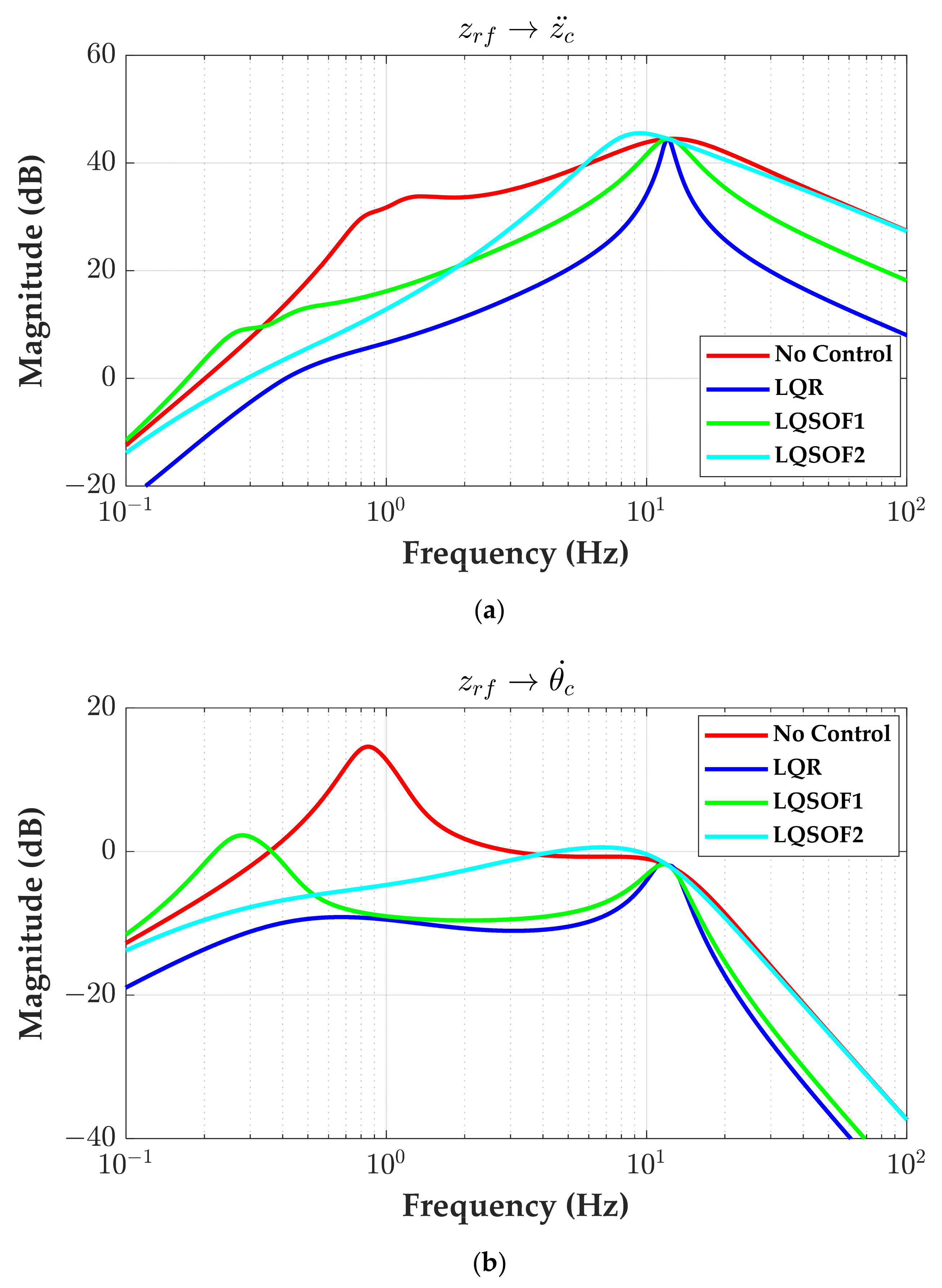
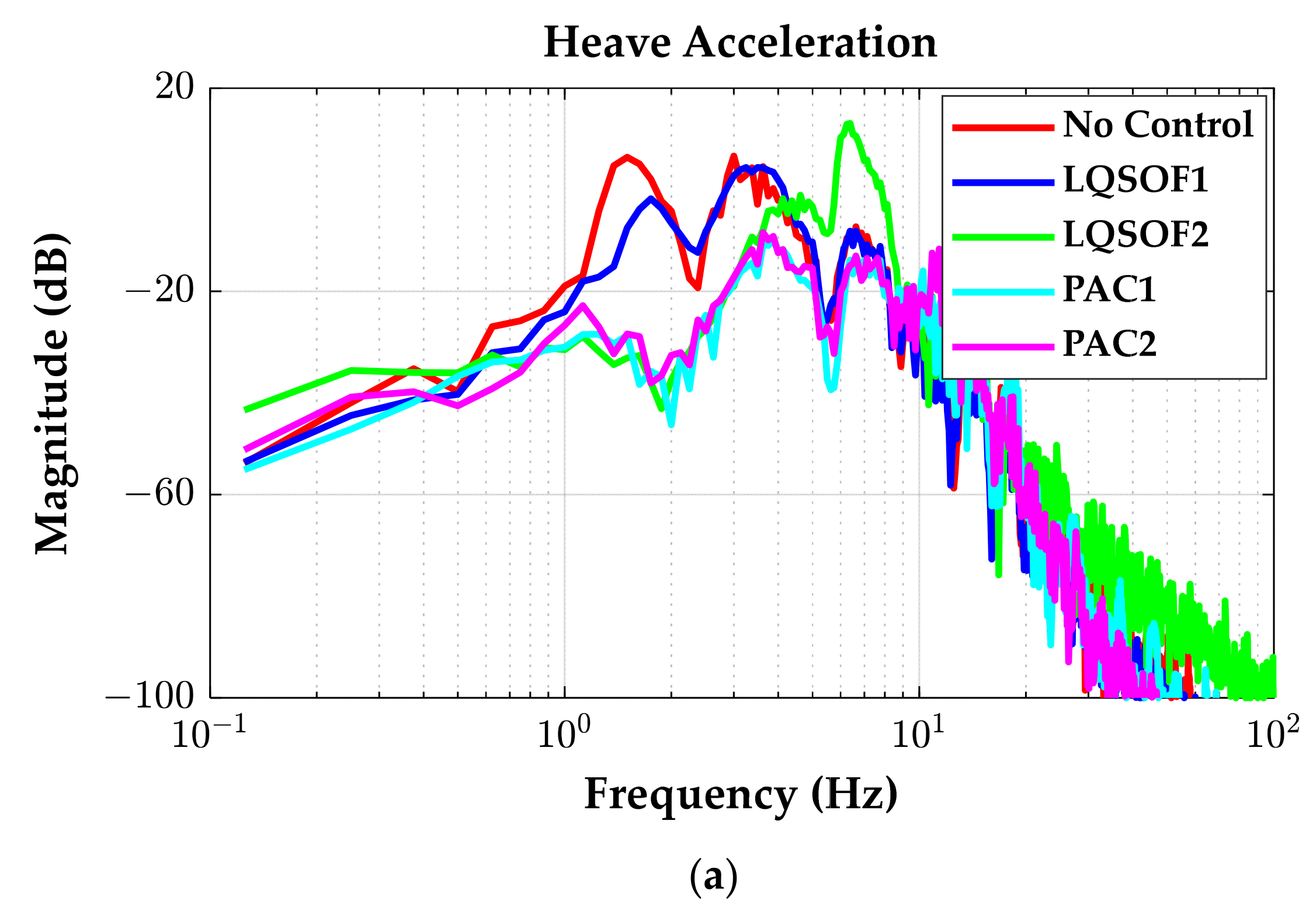
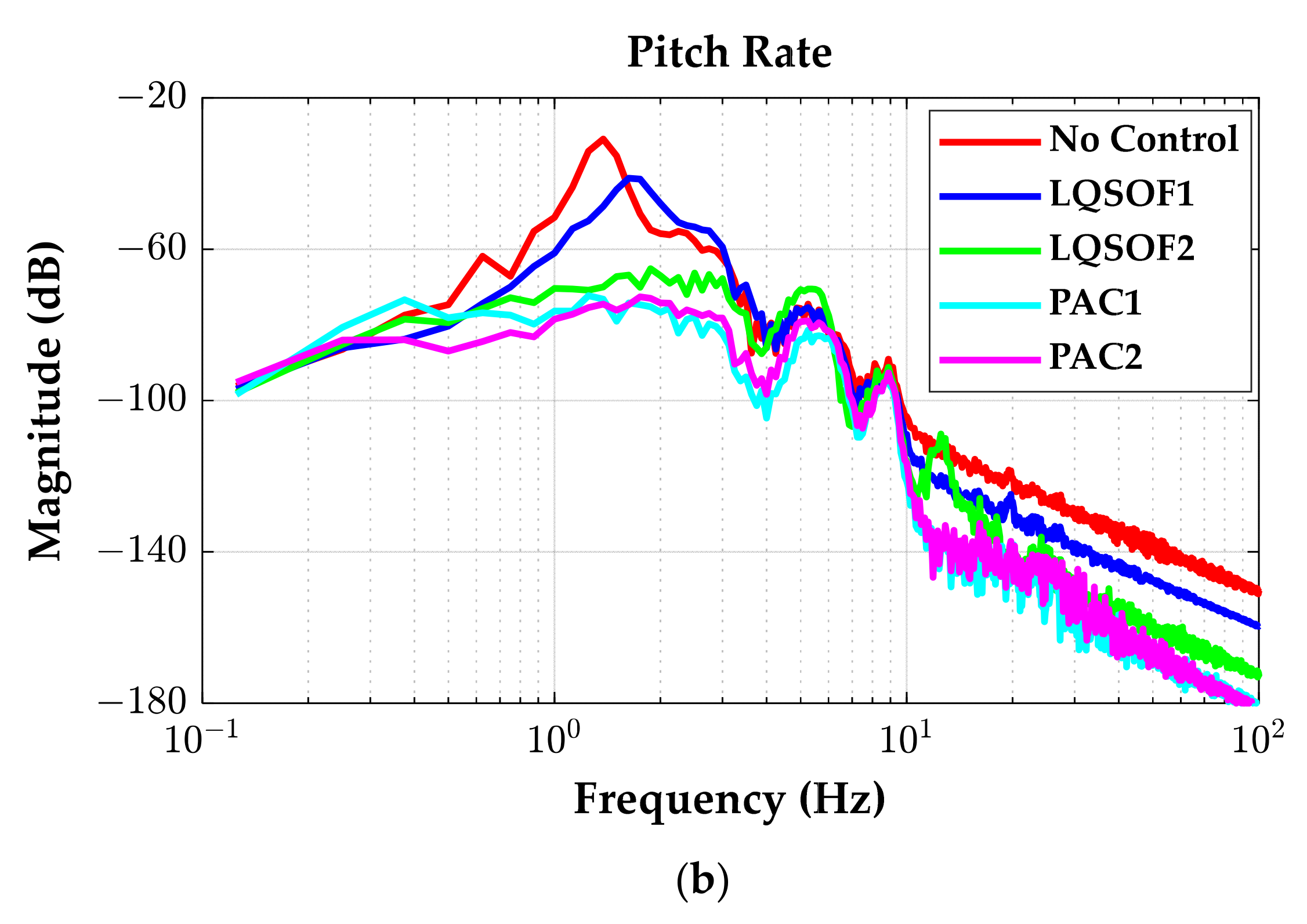
4.2. Frequency Response Analysis with LQ SOF Controllers

With Bryson’s rule and the MAVs presented in Table 1, K_LQR, K_SOF1 and K_SOF2 of LQR, LQSOF1 and LQSOF2 were computed. With the SSEQN and the gain matrices, the frequency response plots from z_rf to a_zc and ω_yc were drawn. Figure 5 shows these plots.

As shown in Figure 5, LQR shows the best performance in respect of RC and MS. It is natural that LQR outperforms LQSOFCs because it uses FSF. On the other hand, LQSOFCs show a worse performance than LQR because those use a smaller number of states. Despite this, LQSOFCs provide a relatively good performance over the frequency range below 5 Hz with respect to a_zc and ω_yc. LQSOF1 outperforms LQSOF2 over 1 Hz in view of a_zc and ω_yc. On the other hand, LQSOF2 outperforms LQSOF1 below 1 Hz. Specifically, LQSOF1 shows poor performance below 0.3 Hz, which does not have an effect on RC and MS.

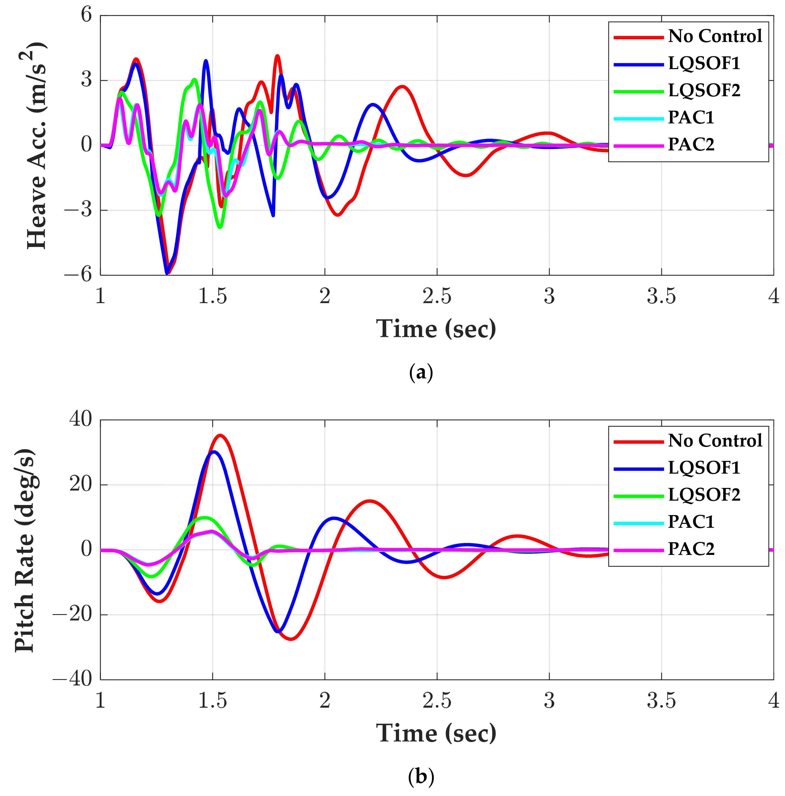
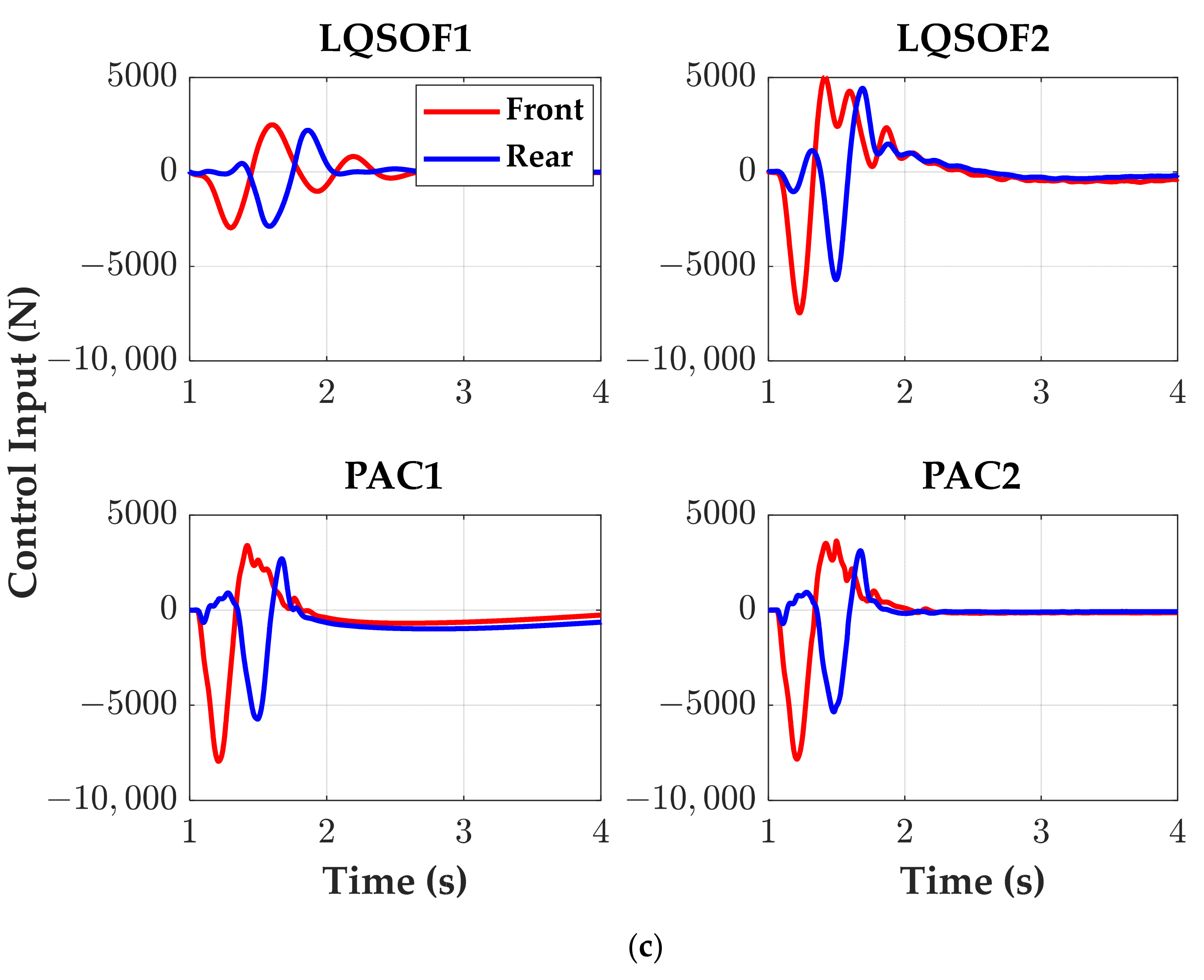
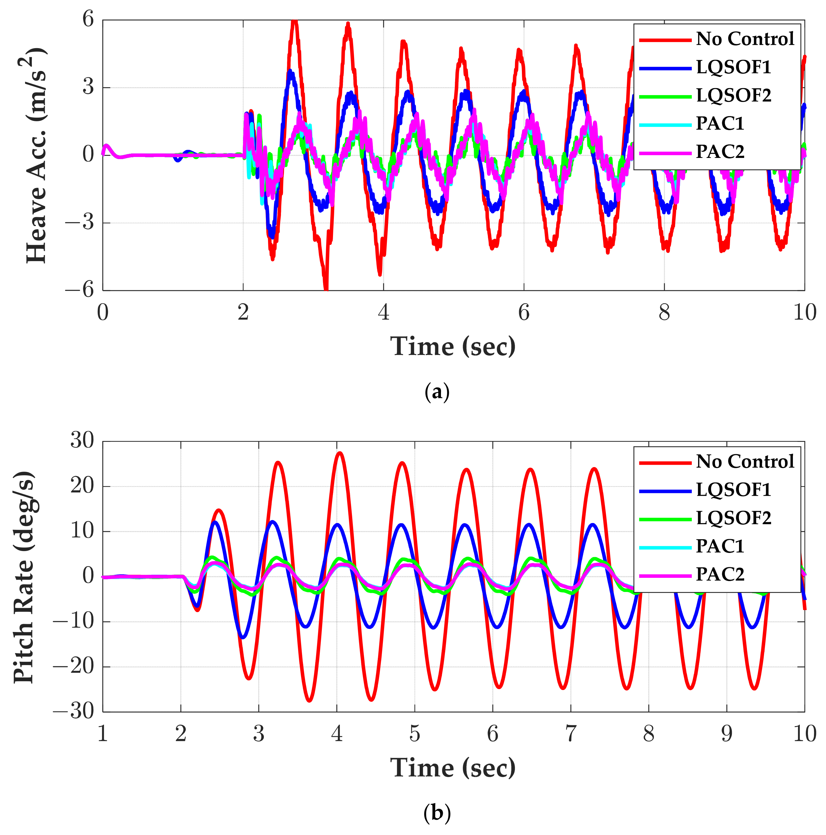
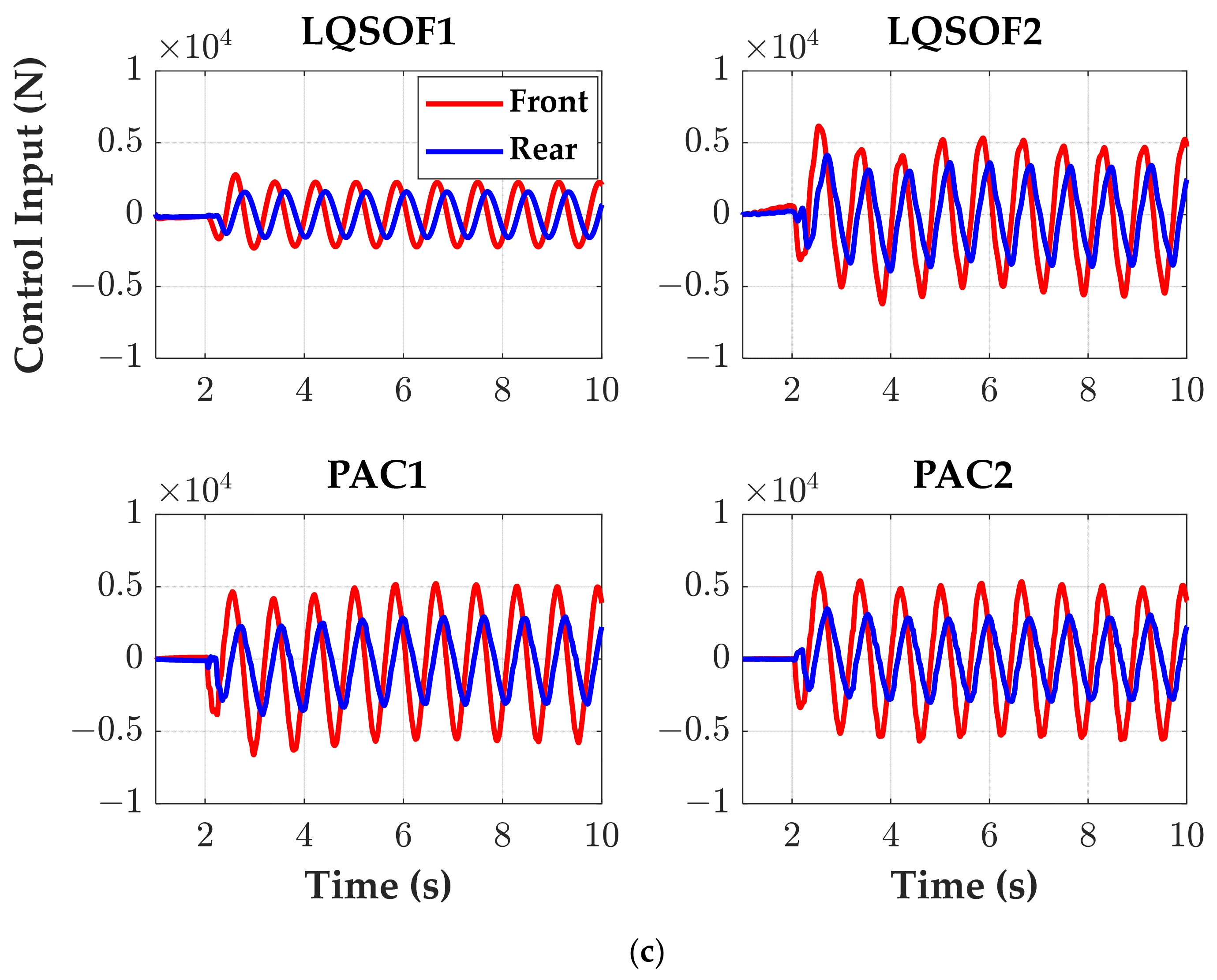
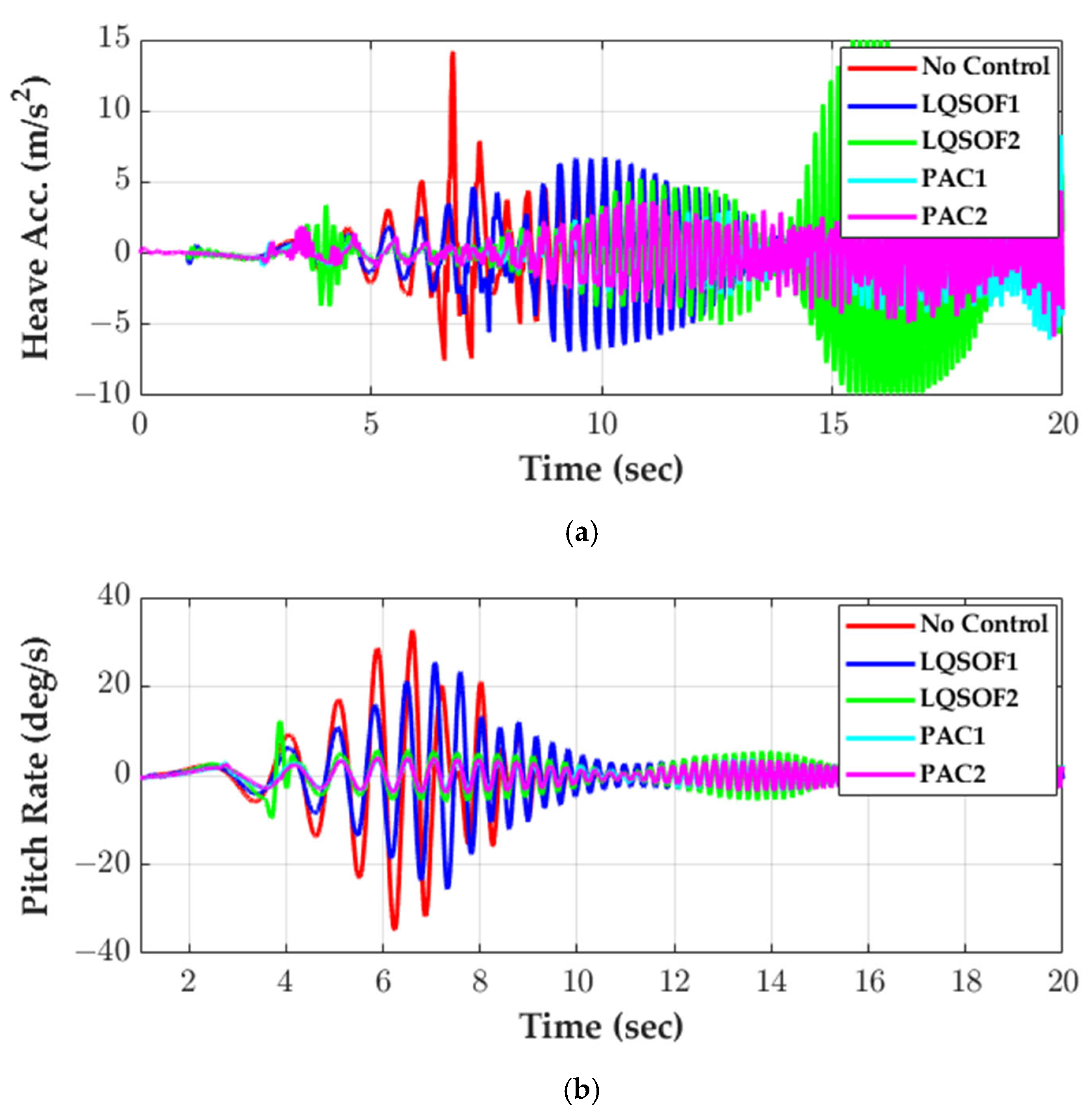
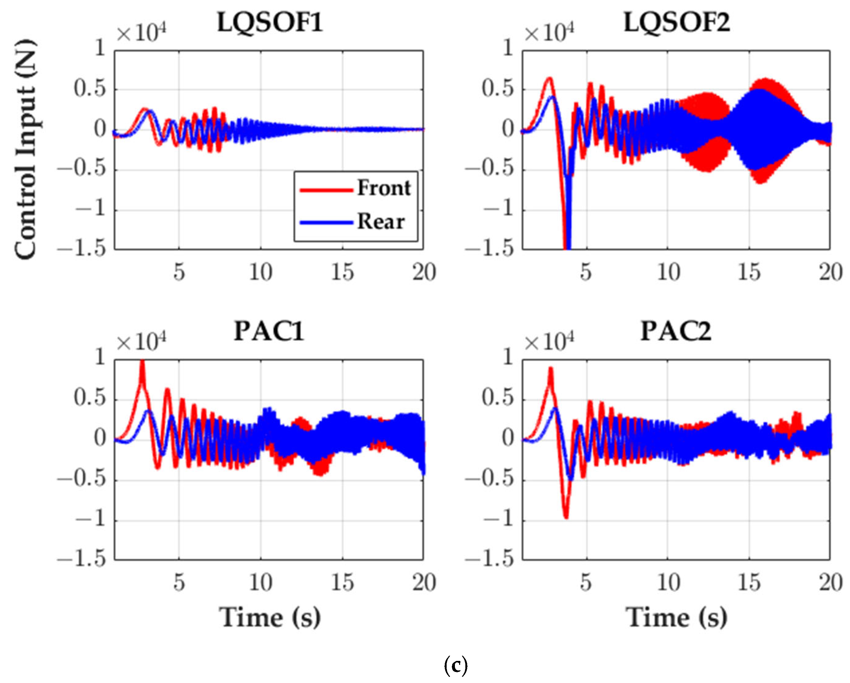
4.3. Simulation with LQ SOF and Parameter Adaptive Conrollers on CarSim

Two LQSOFCs, LQSOF1 and LQSOF2, and two PACs, PAC1 and PAC2, were simulated on CarSim connected to MATLAB/Simulink. The calculation procedure on v_zc and ω_yc given in Figure 3 was implemented in MATLAB/Simulink. When implementing it in MATLAB/Simulink, band-limited white noises were added into the sensor signals measured with Azs_f, Azs_r, Azw_f and Azw_r.

Figure 6 and Figure 7 show the simulation responses of four controllers on the LHSB and SWR, respectively.

Table 2. MAVHAs and MAVPRs obtained from the simulation responses of LQSOFCs and PACs on the LHSB.

Controller	Max |azc| (m/s2)	Max |ωyc| (deg/s)
No Control	5.9	35.2
LQSOF1	5.9 (0%)	30.2 (14%)
LQSOF2	3.8 (36%)	9.9 (72%)
PAC1	2.3 (61%)	5.4 (85%)
PAC2	2.3 (61%)	5.7 (84%)

and

Table 3. MAVHAs and MAVPRs obtained from the simulation responses of LQSOFCs and PACs on the SWR.

Controller	Max |azc| (m/s2)	Max |ωyc| (deg/s)
No Control	4.9	25.0
LQSOF1	3.0 (39%)	11.6 (54%)
LQSOF2	1.5 (69%)	4.1 (84%)
PAC1	1.8 (63%)	2.6 (90%)
PAC2	2.1 (57%)	2.8 (89%)

show the maximums of the absolute values of a_zc and ω_yc (MAVHA and MAVPR) over the simulation period from 1 s to 5 s and from 5 s to 10 s on the LHSB and SWR, respectively. In Table 2 and Table 3, the numbers in the parenthesis stand for the percentage reduction to the no control case. An increased percentage reduction corresponds to improved performance.

As shown in Figure 6 and Figure 7, LQSOF1 shows poor performance in respect of RC and MS. This was not expected from the frequency responses given in Figure 5. This is caused by the fact that there are nonlinearities in springs and dampers in S_f and S_r, and that the magnitudes of signals used for LQSOF1 in CarSim are much smaller than linear model, i.e., SSEQN, when nonlinear spring and dampers are used. For those reasons, the magnitude of the control input for LQSOF1 is much smaller than those of LQSOF2, PAC1 and PAC2. On the other hand, LQSOF2, PAC1 and PAC2 show good performance in respect of RC and MS. Especially, PACs proposed in this paper show much better performance than LQSOFCs. The difference between them originated from the fact that LQSOFCs have constant gains, while PACs adaptively update the gains of SOFCs. From the simulation responses given in Figure 6 and Figure 7, PAC2 is the best controller in respect of RC and MS.

As presented in Table 2, PAC1 and PAC2 provided the reductions of 61% and 61% in relation to a_zc, and the reductions of 85% and 84% in relation to ω_yc, on LHSB and SWR, respectively. Moreover, PAC1 and PAC2 provided the reductions of 63% and 57% in relation to a_zc, and the reductions of 90% and 89% in relation to ω_yc, on LHSB and SWR as presented in Table 3, respectively. These results mean that the parameter adaptive controllers, PAC1 and PAC2, proposed in this paper are quite effective for RC enhancement and MS reduction.

In simulation, the matrices, Χ and Σ, of EKF were set to diag(α,α,α,α) or diag(α,α) and diag(β,β) where α and β were set to 10² and 1, respectively. If α and β are set to 0.1 and 1, it was identified from the simulation result that there are little differences between the previous and current sets of α and β. This is caused by the fact that the system matrix of EKF is the identity, as shown in (34).

Figure 8 shows the simulation responses of LQSOFCs and PACs on the BSSR.

Table 4. MAVHAs and MAVPRs obtained from the simulation responses of LQSOFCs and PACs on the BSSR.

Controller	Max |azc| (m/s2)	Max |ωyc| (deg/s)
No Control	14.2	34.8
LQSOF1	3.5 (75%)	23.5 (33%)
LQSOF2	3.7 (74%)	12.3 (65%)
PAC1	0.9 (94%)	3.6 (90%)
PAC2	1.9 (87%)	4.0 (89%)

shows the MAVHAs and MAVPRs over the simulation period from 1 s to 7 s. Figure 9 shows the frequency responses of LQSOFCs and PACs drawn from the simulation results on the BSSR.

As shown in Figure 8 and Table 4, PAC1 shows the best performance on BSSR. Moreover, PAC1 is better than PAC2 because the former uses four signals and the latter does two signals for control. In contrast to this, LQSOFCs show a relatively worse performance than PACs on BSSR with respect to RC and MS. However, LQSOF2 shows worse performance than the uncontrolled case within the range from 5 to 9 Hz, as shown in Figure 9a. This means that LQSOF2 is not preferred for RC enhancement and MS reduction. As shown in Figure 8a,b, there are fluctuations in the responses of a_zc and ω_yc for PAC2. These deteriorated performance of PAC2. However, PAC2 shows the best performance with respect to a_zc and ω_yc below 5 Hz, as shown in Figure 9. In addition, LQSOFCs and PACs show good performance with respect to ω_yc over 10 Hz.

As presented in Table 4, PAC1 and PAC2 provided the reductions of 94% and 87% in relation to a_zc, and the reductions of 90% and 89% in relation to ω_yc, on BSSR, respectively. These results mean that the parameter adaptive controllers, PAC1 and PAC2, are quite effective on BSSR for RC enhancement and MS reduction.

From the responses obtained on LHSB, SWR and BSSR, it is recommended that PAC1 and PAC2 can be used for RC enhancement and MS reduction. Although PAC1 shows the best performance on LHSB and BSSR, it requires four signals for control. On the contrary, PAC2 requires only two signals and is simpler than PAC1. Although LQSOF2 shows relatively good performance on SWR and BSSR, it shows worse performance than the uncontrolled case within the range from 5 to 9 Hz. This will deteriorate RC and MS. From those results, it can be drawn that PAC2 is recommended for RC enhancement and MS reduction.

5. Conclusions

In this paper, LQSOFCs and PACs were designed and applied to reduce the heave acceleration and the pitch rate of the sprung mass for RC enhancement and MS reduction. HCM was chosen as a vehicle model, and the SSEQN was derived from it. With the SSEQN and LQOF, LQR is designed. To avoid the full-state feedback of LQR which is very difficult to implement in a real vehicle, two types of SOF structure were proposed and optimized with the LQOF by the meta-heuristic method, CMA-ES. PACs were designed with the two SOF structures which are set to make the suspension forces be zero. The PACs updated adaptively the gains of SOF controllers with the extended Kalman filter in every time step. To validate the proposed method regarding RC and MS, the simulation was performed on CarSim. Based on the simulation responses, it was identified that the proposed PACs are quite effective in enhancing RC and reducing MS. It was also shown that PACs are effective on three road profiles.

From simulation responses, the concluding points were identified as follows:

• PACs outperform LQSOFCs on three road profiles. PACs show very good performance below 5 Hz with respect to RC and MS, which is the actuator bandwidth. On the other hand, PAC2 is slightly better than PAC1 because the former uses four signals for control and the latter does two signals. For those reasons, PAC2 is recommended due to its simpler structure and smaller number of sensor signals.
• LQSOF1 shows worse performance than LQSOF2 on LHSB and SWR. This results from the suspension displacements and suspension velocities in CarSim are smaller than those in the linear SSEQN. On the contrary, LQSOF2 show better performance because it uses only the vertical velocity and pitch rate of SPMS. Instead, LQSOF2 shows worse performance than the uncontrolled case within the range from 5 to 9 Hz. In a comprehensive way, LQSOFCs are not recommended for ride comfort enhancement and motion sickness mitigation.

In further research, the performance of the proposed PAC will be verified by experiments on small-scale devices, on hardware-in-the-loop (HIL) environments or on a quarter-car test rig. The procedure to obtain suspension velocities and suspension displacements with accelerometers, as given in Figure 3, can be easily implemented in real vehicles. If a relevant actuator is selected, the proposed method in this paper can be implemented on real vehicles and tested on various scenarios. In addition to the implementation issues, based on the SOF structures proposed in this paper, neural networks or reinforcement learning will be applied for RC enhancement and MS reduction. This is a natural consequence due to the fact that RLS, EKF, neural networks and reinforcement learning are learning-based algorithms.

References

1. Hrovat, D. Survey of advanced suspension developments and related optimal control applications. Automatica 1997, 33, 1781–1817. [Google Scholar] [CrossRef]
2. Cao, D.; Song, X.; Ahmadian, M. Editors’ perspectives: Road vehicle suspension design, dynamics, and control. Veh. Syst. Dyn. 2011, 49, 3–28. [Google Scholar] [CrossRef]
3. Poussot-Vassal, C.; Spelta, C.; Sename, O.; Savaresi, S.M.; Dugard, L. Survey and performance evaluation on some automotive semi-active suspension control methods: A comparative study on a single-corner model. Annu. Rev. Control 2012, 36, 148–160. [Google Scholar] [CrossRef]
4. Tseng, H.E.; Hrovat, D. State of the art survey: Active and semi-active suspension control. Veh. Syst. Dyn. 2015, 53, 1034–1062. [Google Scholar] [CrossRef]
5. Theunissen, J.; Tota, A.; Gruber, P.; Dhaens, M.; Sorniotti, A. Preview-based techniques for vehicle suspension control: A state-of-the-art review. Annu. Rev. Control 2021, 51, 206–235. [Google Scholar] [CrossRef]
6. Tang, Q.; Xiang, H.; Cheng, J.; Xiao, X.; Yu, W.; Zhang, S.; Tang, B.; Ghu, G. Study on evaluation method of motion sickness in electric vehicles. In Proceedings of the 2024 8th CAA International Conference on Vehicular Control and Intelligence, CVCI 2024, Chongqing, China, 25–27 October 2024. [Google Scholar]
7. Shi, Z.; He, L.; Wang, M.; Bian, Y.; Cui, S.; Chen, P. Ideal comfort ellipses and comfort dynamics model for mitigating motion sickness in battery electric vehicle. Veh. Syst. Dyn. 2025, OnlineFirst. [Google Scholar] [CrossRef]
8. Deng, Z.; Yuan, K.; Xiao, X. Investigative examination of motion sickness indicators for electric vehicles. Proc. Inst. Mech. Eng. Part D J. Automob. Eng. 2025, OnlineFirst. [Google Scholar] [CrossRef]
9. Dam, A.; Jeon, M. A review of motion sickness in automated vehicles. In Proceedings of the AutomotiveUI ‘21: 13th International Conference on Automotive User Interfaces and Interactive Vehicular Applications, Leeds, UK, 9–14 September 2021; pp. 39–48. [Google Scholar]
10. Asua, E.; Gutiérrez-Zaballa, J.; Mata-Carballeira, O.; Ruiz., J.A.; del Campo, I. Analysis of the motion sickness and the lack of comfort in car passengers. Appl. Sci. 2022, 12, 3717. [Google Scholar] [CrossRef]
11. Kirst, L.; Ernst, B.; Kern, A.; Steinhauser, M. The Problem of motion sickness and its implications for automated driving. In User Experience Design in the Era of Automated Driving; Riener, A., Jeon, M., Alvarez, I., Eds.; Studies in Computational Intelligence; Springer: Cham, Switzerland, 2022; Volume 980. [Google Scholar]
12. Irmak, T.; Pool, D.M.; de Winkel, K.N.; Happee, R. Validating models of sensory conflict and perception for motion sickness prediction. Biol. Cybern. 2023, 117, 185–209. [Google Scholar] [CrossRef]
13. Pereira, E.; Macedo, H.; Lisboa, I.C.; Sousa, E.; Machado, D.; Silva, E.; Coelho, V.; Arezes, P.; Costa, N. Motion sickness countermeasures for autonomous driving: Trends and future directions. Transp. Eng. 2024, 15, 100220. [Google Scholar] [CrossRef]
14. Xie, W.; He, D.; Wu, G. Inducers of motion sickness in vehicles: A systematic review of experimental evidence and meta-analysis. Transp. Res. Part F Traffic Psychol. Behav. 2023, 99, 167–188. [Google Scholar] [CrossRef]
15. Diels, C.; Ye, Y.; Bos, J.; Maeda, S. Motion sickness in automated vehicles: Principal research questions and the need for common protocols. SAE Int. J. Connect. Autom. Veh. 2022, 5, 121–134. [Google Scholar] [CrossRef]
16. Zhang, Y.; Zhao, H.; Hu, C.; Tian, Y.; Li, Y.; Jiao, X. Mitigation of motion sickness and optimization of motion comfort in autonomous vehicles: Systematic survey. IEEE Trans. Intell. Trans. Sys. 2024, 25, 21737–21756. [Google Scholar] [CrossRef]
17. Jeong, Y.; Yim, S. Design of active suspension controller for ride comfort enhancement and motion sickness mitigation. Machines 2024, 12, 254. [Google Scholar] [CrossRef]
18. Kim, J.; Yim, S. Design of static output feedback suspension controllers for ride comfort improvement and motion sickness reduction. Processes 2024, 12, 968. [Google Scholar] [CrossRef]
19. Kim, J.; Yim, S. Design of a suspension controller with an adaptive feedforward algorithm for ride comfort enhancement and motion sickness mitigation. Actuators 2024, 13, 315. [Google Scholar] [CrossRef]
20. Kim, J.; Yim, S. Design of a suspension controller with human body model for ride comfort improvement and motion sickness mitigation. Actuators 2024, 13, 520. [Google Scholar] [CrossRef]
21. Oh, H.E.; Park, D.J.; Park, J.P.; Ahn, S.J.; Jeong, W.B. Digital filter design of frequency weighting function to measure and assess human vibration. Noise Control Eng. J. 2017, 65, 183–190. [Google Scholar] [CrossRef]
22. Medina Santiago, A.; Orozco Torres, J.A.; Hernández Gracidas, C.A.; Garduza, S.H.; Franco, J.D. Diagnosis and study of mechanical vibrations in cargo vehicles using ISO 2631-1:1997. Sensors 2023, 23, 9677. [Google Scholar] [CrossRef]
23. Ekchian, J.; Graves, W.; Anderson, Z.; Giovanardi, M.; Godwin, O.; Kaplan, J.; Ventura, J.; Lackner, J.R.; DiZio, P. A High-Bandwidth Active Suspension for Motion Sickness Mitigation in Autonomous Vehicles. In Proceedings of the SAE 2016 World Congress and Exhibition, Detroit, MI, USA, 13 April 2016; SAE Technical Paper 2016-01-1555. SAE International: Warrendale, PA, USA, 2016. [Google Scholar]
24. DiZio, P.; Ekchian, J.; Kaplan, J.; Ventura, J.; Graves, W.; Giovanardi, M.; Anderson, Z.; Lackner, J.R. An active suspension system for mitigating motion sickness and enabling reading in a car. Aerosp. Med. Hum. Perform. 2018, 89, 822–829. [Google Scholar] [CrossRef]
25. Camino, J.F.; Zampieri, D.E.; Peres, P.L.D. Design of a vehicular suspension controller by static output feedback. In Proceedings of the American Control Conference, San Diego, CA, USA, 2–4 June 1999; pp. 3168–3171. [Google Scholar]
26. Zhao, J.; Wang, X.; Wong, P.K.; Xie, Z.; Jia, J.; Li, W. Multi-objective frequency domain-constrained static output feedback control for delayed active suspension systems with wheelbase preview information. Nonlinear Dyn. 2021, 103, 1757–1774. [Google Scholar] [CrossRef]
27. Mrazgua, J.; Chaibi, R.; Tissir, E.H.; Ouahi, M. Static output feedback stabilization of T-S fuzzy active suspension systems. J. Terramechanics 2021, 97, 19–27. [Google Scholar] [CrossRef]
28. Behrouz, H.; Mohammadzaman, I.; Mohammadi, A. Robust static output feedback H2/H control synthesis with pole placement constraints: An LMI approach. Int. J. Control Autom. Syst. 2021, 19, 241–254. [Google Scholar] [CrossRef]
29. Park, M.; Yim, S. Design of static output feedback and structured controllers for active suspension with quarter-car model. Energies 2021, 14, 8231. [Google Scholar] [CrossRef]
30. Jeong, Y.; Shon, Y.; Chang, S.; Yim, S. Design of static output feedback controllers for an active suspension system. IEEE Access 2022, 10, 26948–26964. [Google Scholar] [CrossRef]
31. Elias, L.J.; Faria, F.A.; Araujo, R.; Magossi, R.F.Q.; Oliveira, V.A. Robust static output feedback H control for uncertain Takagi–Sugeno fuzzy systems. IEEE Trans. Fuzzy Syst. 2022, 30, 4434–4446. [Google Scholar] [CrossRef]
32. Hansen, N.; Muller, S.D.; Koumoutsakos, P. Reducing the time complexity of the derandomized evolution strategy with covariance matrix adaptation (CMA-ES). Evol. Comput. 2003, 11, 1–18. [Google Scholar] [CrossRef]
33. Hansen, N. The CMA evolution strategy: A comparing review. In Towards a New Evolutionary Computation. Advances in Estimation of Distribution Algorithms; Lozano, J.A., Larrañga, P., Inza, I., Bengoetxea, E., Eds.; Springer: Berlin/Heidelberg, Germany, 2006; pp. 75–102. [Google Scholar]
34. Pan, H.; Sun, W.; Jing, X.; Gao, H.; Yao, J. Adaptive tracking control for active suspension systems with non-ideal actuators. J. Sound Vib. 2017, 399, 2–20. [Google Scholar] [CrossRef]
35. Huang, Y.; Na, J.; Wu, X.; Gao, G.; Guo, Y. Robust adaptive control for vehicle active suspension systems with uncertain dynamics. Trans. Inst. Meas. Control. 2018, 40, 1237–1249. [Google Scholar] [CrossRef]
36. Mozaffari, A.; Chenouri, S.; Qin, Y.; Khajepour, A. Learning-based vehicle suspension controller design: A review of the state-of-the-art and future research potentials. eTransportation 2019, 2, 100024. [Google Scholar] [CrossRef]
37. Liu, Y.; Zhang, Y.; Liu, L.; Tong, S.; Chen, C.L.P. Adaptive finite-time control for half-vehicle active suspension systems with uncertain dynamics. IEEE/ASME Trans. Mechatron. 2021, 26, 168–178. [Google Scholar]
38. Yim, S. Comparative study on active suspension controllers with parameter adaptive and static output feedback control. Actuators 2025, 14, 150. [Google Scholar] [CrossRef]
39. Haykin, S. Adaptive Filter Theory, 2nd ed.; Prentice-Hall: Hoboken, NJ, USA, 1991; pp. 760–761. [Google Scholar]
40. Wan, E.A.; Nelson, A.T. Dual extended Kalman filter methods. In Kalman Filtering and Neural Networks; Haykin, S., Ed.; JohnWiley & Sons: NewYork, NY, USA, 2001; Chapter 5. [Google Scholar]
41. Wenzel, T.A.; Burnham, K.J.; Blundell, M.V.; Williams, R.A. Dual extended Kalman filter for vehicle state and parameter estimation. Veh. Syst. Dyn. 2006, 44, 153–171. [Google Scholar] [CrossRef]
42. Zhang, F.; Wang, Y.; Hu, J.; Yin, G.; Chen, S.; Zhang, H.; Zhou, D. A novel comprehensive scheme for vehicle state estimation using dual extended H-Infinity Kalman filter. Electronics 2021, 10, 1526. [Google Scholar] [CrossRef]
43. Wu, M.; Qin, L.; Wu, G. State of charge estimation of power lithium-ion battery based on an adaptive time scale dual extend Kalman filtering. J. Energy Storage 2021, 39, 102535. [Google Scholar]
44. Ok, M.; Ok, S.; Park, J.H. Estimation of vehicle attitude, acceleration, and angular velocity using convolutional neural network and dual extended Kalman filter. Sensors 2021, 21, 1282. [Google Scholar] [CrossRef]
45. Wei, W.; Dourra, H.; Zhu, G. Vehicle tire traction torque estimation using a dual extended Kalman filter. J. Dyn. Sys. Meas. Control 2022, 144, 031004. [Google Scholar] [CrossRef]
46. Bryson, A.E., Jr.; Ho, Y. Applied Optimal Control; Hemisphere: New York, NY, USA, 1975. [Google Scholar]
47. Sadabadia, M.S.; Peaucelleb, D. From static output feedback to structured robust static output feedback: A survey. Annu. Rev. Control. 2016, 42, 11–26. [Google Scholar] [CrossRef]
48. Khan, M.; Sun, H.; Xiang, Y.; Shi, D. Electric vehicles participation in load frequency control based on mixed H2/H. Int. J. Electr. Power Energy Syst. 2021, 125, 106420. [Google Scholar]
49. Rodrigues, L. From LQR to static output feedback: A new LMI approach. In Proceedings of the 2022 IEEE 61st Conference on Decision and Control (CDC), Cancun, Mexico, 6–9 December 2022. [Google Scholar]
50. Yang, Y.; Liu, C.; Chen, L.; Zhang, X. Phase deviation of semi-active suspension control and its compensation with inertial suspension. Acta Mech. Sin. 2024, 40, 523367. [Google Scholar] [CrossRef]
51. Liu, S.; Zhang, L.; Liu, Y.; Wang, J.; Yang, C.; Zhang, J. Motion posture control of corner module architecture intelligent electric vehicle on deep-potholed roads. IEEE/ASME Trans. Mechatron. 2024, 29, 4480–4491. [Google Scholar] [CrossRef]
52. Liu, S.; Zhang, L.; Chen, M.; Yang, C.; Zhang, J.; Wang, J. Multiple suspensions coordinated control for corner module architecture intelligent electric vehicles on stepped roads. IEEE Trans. Intell. Veh. 2025, EarlyAccess. [Google Scholar] [CrossRef]
53. Mechanical Simulation Corporation. CarSim Data Manual, 8th ed.; Mechanical Simulation Corporation: Ann Arbor, MI, USA, 2009. [Google Scholar]
Figure 1. Frequency weightings given in ISO 2631-1 [21] and presented by Dizio [23,24].
Applsci 15 04977 g001
Figure 2. Half-car model with front and rear suspensions.
Applsci 15 04977 g002
Figure 3. Block diagram for calculation on the signals for SOFCs.
Applsci 15 04977 g003
Figure 4. Bounce sine sweep road profile.
Applsci 15 04977 g004
Figure 5. Frequency responses of LQR and LQSOFCs. (a) from zrf to azc; (b) from zrf to ωyc.
Applsci 15 04977 g005
Figure 6. Simulation responses of LQSOFCs and PACs on the LHSB. (a) azc; (b) ωyc; (c) uf and ur.
Applsci 15 04977 g006aApplsci 15 04977 g006b
Figure 7. Simulation responses of LQSOFCs and PACs on the SWR. (a) azc; (b) ωyc; (c) uf and ur.
Applsci 15 04977 g007aApplsci 15 04977 g007b
Figure 8. Simulation responses of LQSOFCs and PACs on the BSSR. (a) azc; (b) ωyc; (c) uf and ur.
Applsci 15 04977 g008aApplsci 15 04977 g008b
Figure 9. Frequency responses of LQSOFCs and PACs on the BSSR. (a) azc; (b) ωyc.
Applsci 15 04977 g009aApplsci 15 04977 g009b