Robust Grey Relational Analysis-Based Accuracy Evaluation Method

Abstract

The conventional grey relational analysis (GRA) demonstrates limitations in dynamic simulation data evaluation due to its failure to simultaneously account for geometric similarity among dynamic indicators and the proximity of data curve distances. This deficiency manifests as a compromised robustness in noise resistance and interference suppression, consequently leading to discrepancies between model accuracy and practical scenarios. To address these shortcomings, this paper proposes a robust grey relational analysis-based accuracy evaluation method (RGRA-AEM). The methodology incorporates the expected penetration rate to facilitate interpolation computation and employs deviation acceptability as a distance threshold indicator. By integrating the grey relational degree, mean squared deviation distance, and accuracy modeling, this approach achieves enhanced stability in accuracy assessment. It effectively mitigates the inherent weakness of traditional GRA that overemphasizes sequential curve similarity while significantly improving the anti-noise performance and interference resistance of grey relational coefficients. Experimental validation through the internal ballistic test-simulation dynamic data of a hybrid rocket motor conclusively demonstrates the superior robustness of the proposed methodology.

1. Introduction

The development process of advanced equipment systems is typically characterized by high costs, small-sample constraints, and compressed development cycles. As an indispensable experimental methodology, simulation testing permeates the entire development lifecycle from conceptual design to system finalization. Although computational models are engineered to emulate physical systems with high fidelity, non-negligible divergences in their dynamic behavioral profiles. To ensure the validity and applicability of simulation results, it is imperative to conduct quantitative accuracy assessments of simulation models. This evaluation process enables systematic verification of model fidelity and establishes a scientific foundation for result interpretation and engineering decision-making throughout the equipment development process [1,2].

Accuracy evaluation constitutes a critical component in the construction of simulation models and systems. Distinct simulation model metrics necessitate tailored accuracy assessment methodologies. For dynamic data analysis employing temporal sequence characteristics, grey relational analysis (GRA) [3,4,5] emerges as an effective approach. This method quantifies the spatial consistency of geometric patterns between data sequences through grey relational degree computation, thereby analyzing inter-sequence correlations. Serving as a robust tool for simulation accuracy verification, GRA facilitates the quantification of geometric congruence among dynamic data trajectories, enabling the systematic evaluation of model fidelity in time-dependent simulation scenarios [6,7,8].

Grey relational analysis demonstrates significant advantages in synthesizing multi-dimensional indicator information to deliver comprehensive evaluation outcomes. By virtue of its capability to holistically integrate heterogeneous data attributes, this methodology effectively addresses the limitations of single-weighting approaches in indicator prioritization. Within the context of dynamic modulus prediction models, GRA is recognized as a methodologically robust framework, exhibiting enhanced reliability and practical applicability. Its inherent capacity to reconcile geometric pattern consistency with quantitative correlation analysis ensures a rigorous validation of model outputs, thereby overcoming limitations inherent in conventional unidimensional evaluation paradigms [9].

In the study of grey relational analysis, it has been found that grey relational degrees have limitations in ordinal preservation [10,11,12,13]. And due to the dependence of grey relational analysis on the geometric similarity between data to determine the degree of correlation, there are limitations in the processing of data with highly nonlinear features; moreover, grey relational analysis may be affected by data distribution and sample size when determining weights, which may lead to inaccurate weight allocation in some cases, difficulty in accurately reflecting the true correlation between factors in situations with small data volume or low data quality, and may affect the predictive ability of the model [14,15,16]. This leads to poorer robustness of the grey relational analysis method against noise and disturbances. Simply adjusting parameters such as the relational coefficient and resolution coefficient in hopes of achieving an approximation between simulation results and actual test results may adversely affect the reliability assessment and applicability of the model; in addition, traditional GRA models are mostly constructed based on sample matrices, and changes in the way the sample matrices are constructed will affect the stability of the results, and most of the models only describe the features from the perspectives of local distances and slopes, which makes it difficult to reflect the overall trend when the data are dispersed [17,18,19,20]. This can result in predictive deviations and limitations in subsequent model evaluations and practical applications [21,22].

Among the accuracy assessment methods of gray system theory, there are limitations in each method. For example, the gray correlation analysis model mentioned in reference [19] can effectively deal with “weak information” and “gray nature” data; however, it has certain requirements on the statistical characteristics of the data and the sample size, and the reliability of the results is affected when the non-statistical pattern of the data is obvious or the sample size is insufficient. Reference [23] highlighted that the standardization method in the calculation of grey relative occurrence has a great impact on the test results, and the original standardization method is prone to increasing the weight of the initial data and reducing the accuracy of the results. Although the multivariate gray prediction model in reference [24] has been improved in various ways, traditional models such as GM(1,1) are underperforming in multivariate interaction scenarios, and the MGM(1,n) model has an inherent error mechanism that affects the accuracy of simulated predictions. Overall, the existing accuracy assessment methods need to be improved in model construction, data processing, and result validation, and they need to be flexibly selected and improved according to specific problems and data characteristics in order to improve the reliability of the assessment results.

Compared to the previous methods, the proposed method has lower computational complexity and less difficulty in model construction. Unlike previous methods, the proposed method incorporates both an enhanced interpolation mechanism and bias tolerance control to improve robustness to noise and perturbation and incorporates the effect of relative distance between sequences on accuracy assessment taking into account the sequence geometry instead of relying solely on metrics such as mean deviation, percentage error, and geometric variation for accuracy assessment. For instance, the Mean Absolute Percentage Error (MAPE) is very sensitive to cases where the actual value is close to zero because it is calculated based on a percentage of the actual value, which can result in an infinitely magnified error. In addition, MAPE may have computational problems or lose its meaning when dealing with zero or negative data. Mean Absolute Error (MAE) fails to reflect the direction of the prediction error, i.e., it cannot distinguish whether the error is due to overestimation or underestimation. Also, because MAE treats all errors equally and does not consider the distribution of error sizes, it may not adequately reflect the true performance of the model in the presence of large but sparse errors. And in contrast to the accuracy assessment under traditional gray correlation analysis, the proposed bias acceptability approach enhances the traditional gray correlation analysis through a two-scale framework: microscopically, it locally adjusts the correlation coefficients of the data points within the error tolerance while preserving the original data distribution and fitting accuracy, and macroscopically, it amplifies the distance weights by strategically selecting sequence points. This coordinated approach addresses local perturbation uncertainty through targeted coefficient corrections, adapts to real-world noise complexity through macroscopic pattern enhancement, and systematically improves model robustness through synergistic micro–macro interactions, thus achieving superior stability and reliability when dealing with noisy time series datasets.

This paper addresses the drawback of poor robustness in grey relational analysis by introducing the expected valve crossing rate and combining it with interpolation functions to calculate the sequence distance correction points. It proposes a deviation acceptability control metric to filter and screen time series data, constructs a distance weighting function, and combines this with the grey relational degree—mean square deviation distance—accuracy model to achieve accuracy assessment. Finally, it verifies the approach using an example of dynamic data from experiments and simulations.

2. Accuracy Assessment Based on GRA

The principle of accuracy assessment based on grey relational analysis involves constructing a grey relational degree-mean square deviation distance model and an accuracy-mean square deviation distance model. The simulation test data and physical test data are substituted into the grey relational degree-mean square deviation distance model. The resulting mean square deviation distances are then converted into accuracy values through the mean square deviation distance–accuracy model.

2.1. Calculation of Grey Relational Degrees and Mean Square Deviation Distances

Let the reference time series data measured by physical tests at equal time intervals be given as $\mathit{X}=(x_1,x_2,\cdots ,x_n)$, the time series data generated by the simulation model is $\mathit{Y}=(y_1,y_2,\cdots ,y_n)$; the grey correlation of two time series is calculated as follows:

$$\gamma (\mathit{X},\mathit{Y})={\displaystyle \frac{1}{n}}{\displaystyle \sum _{i=1}^n\frac{\underset{i}{\min } |x_i-y_i|+\tau \underset{i}{\max } |x_i-y_i|}{|x_i-y_i|+\tau \underset{i}{\max } |x_i-y_i|}}$$

(1)

here, $\gamma (\mathit{X},\mathit{Y})$ denotes the grey correlation between time series $\mathit{X}$ and $\mathit{Y}$; $\underset{i}{\min } |x_i-y_i|$ and $\underset{i}{\max } |x_i-y_i|$, respectively, represent the minimum and maximum values of the absolute difference between data points $x_i$ and $y_i$; $\tau$ is the resolution coefficient; $\tau \in \left[0,1\right]$ determines the influence of grey correlation by the maximum distance $\underset{i}{\max } |x_i-y_i|$ according to the theory of grey correlation space proposed by Julong Deng, taking into account the overall correlation and anti-interference effect; $\tau$ usually take 0.5 [25].

According to the characteristics of the grey relational degree coefficient, the higher the grey relational degree, the greater the consistency between the simulation output time series and the reference data; conversely, the lower the grey relational degree, the lesser the consistency between the simulation output time series and the reference data [26].

Depending on the need to construct the grey relational degree-mean square deviation distance model later, the mean square deviation distance $d(\mathit{X},\mathit{Y})$ between two time series is given as follows:

$$d(\mathit{X},\mathit{Y})=\sqrt{{\displaystyle \frac{1}{n}}{\displaystyle \sum _{i=1}^n{(x_i-y_i)}^2}}$$

(2)

here, $x_i$ and $y_i$ denotes the sampling point of the time series $\mathit{X}$ and $\mathit{Y}$.

According to Yugang Sun’s research on grey relational analysis, a threshold value for the mean square deviation distance is introduced, denoted as $d_{ref}$, called the reference mean square distance. When $d(\mathit{X},\mathit{Y})>d_{ref}$, the consistency and accuracy between $\mathit{X}$ and $\mathit{Y}$ are low, which indicates that there is a significant discrepancy between $\mathit{X}$ and $\mathit{Y}$, suggesting that the degree of agreement or similarity is not high, and, consequently, the accuracy is also low. When $d(\mathit{X},\mathit{Y})<d_{ref}$, the consistency and accuracy between $\mathit{X}$ and $\mathit{Y}$ are high.

Define $d_{\max }$ as the maximum mean square deviation distance between $\mathit{X}$ and $\mathit{Y}$ at any time t, which is referred to as the upper limit of the mean square deviation distance. Define $d_{\min }$ as the minimum mean square deviation distance between $\mathit{X}$ and $\mathit{Y}$ at any time t, which is referred to as the lower limit of the mean square deviation distance.

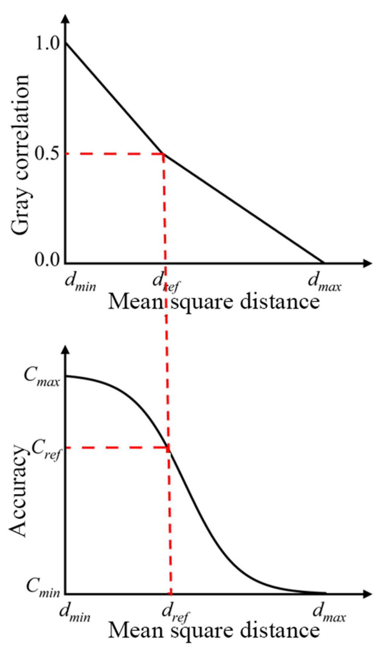
2.2. Grey Relational Degree-Mean Square Deviation Distance Model

The reference grey relational degree ${\gamma }_{ref}$ is determined jointly by the selected relational degree model and the actual requirements. The higher its value, the greater the requirement for model consistency. When converting from grey relational degree to accuracy, the changes in accuracy near the reference grey relational degree become smoother.

To link the grey relational coefficient with the mean square deviation, we introduce some intermediary variables, define the grey relational degree corresponding to the upper limit of the mean square deviation distance as ${\gamma }_{\min }$, termed the minimum grey relational degree, and define the grey relational degree corresponding to the lower limit of the mean square deviation distance as ${\gamma }_{\max }$, termed the maximum grey relational degree.

To represent the relationship between the grey relational degree and the mean square deviation distance, define the reference grey relational degree ${\gamma }_{ref}$ corresponding to the reference mean square deviation distance $d_{ref}$. When $\gamma (\mathit{X},\mathit{Y})>{\gamma }_{ref}$, the consistency between $\mathit{X}$ and $\mathit{Y}$ are high. When $\gamma (\mathit{X},\mathit{Y})<{\gamma }_{ref}$, the consistency between $\mathit{X}$ and $\mathit{Y}$ are high. According to Li Yuning’s research, for the ideal standard model, take ${\gamma }_{ref}=0.5$ [12].

Consequently, $\gamma (\mathit{X},\mathit{Y})\in [{\gamma }_{ref},{\gamma }_{\max }]$ corresponds to $d(\mathit{X},\mathit{Y})\in (d_{\min },d_{ref})$, as $\gamma (\mathit{X},\mathit{Y})\in [{\gamma }_{\min },{\gamma }_{ref}]$ is equivalent to $d(\mathit{X},\mathit{Y})\in (d_{ref},d_{\max })$, and $\gamma (\mathit{X},\mathit{Y})$ has a linear relationship with $d(\mathit{X},\mathit{Y})$. Accordingly, the grey relational degree—mean square deviation distance model is established as follows:

$$\left\{\begin{array}{l}{\displaystyle \frac{d_{\min }-d_{ref}}{{\gamma }_{\max }-{\gamma }_{ref}}}={\displaystyle \frac{d(\mathit{X},\mathit{Y})-d_{ref}}{\gamma (\mathit{X},\mathit{Y})-{\gamma }_{ref}}}\hspace{1em}\hspace{1em}if \gamma (\mathit{X},\mathit{Y})\in \left({\gamma }_{ref},{\gamma }_{\max }\right)\\ {\displaystyle \frac{d_{ref}-d_{\max }}{{\gamma }_{ref}-{\gamma }_{\min }}}={\displaystyle \frac{d_{ref}-d(\mathit{X},\mathit{Y})}{{\gamma }_{ref}-\gamma (\mathit{X},\mathit{Y})}}\hspace{1em}\hspace{1em}if \gamma (\mathit{X},\mathit{Y})\in \left({\gamma }_{\min },{\gamma }_{ref}\right)\end{array}\right.$$

(3)

here, $d(\mathit{X},\mathit{Y})$ is the mean square deviation distance between $\mathit{X}$ and $\mathit{Y}$; $\gamma (\mathit{X},\mathit{Y})$ is the grey relational degree between $\mathit{X}$ and $\mathit{Y}$; ${\gamma }_{\min }$ is the minimum grey relational degree; ${\gamma }_{\max }$ is the maximum grey relational degree; ${\gamma }_{ref}$ is the reference grey relational degree; $d_{ref}$ is the reference mean square deviation distance.

2.3. The Mean Square Deviation Distance–Accuracy Model

Further, we need to construct a mean-variance distance–accuracy model to further map the gray correlation to accuracy via the mean-variance distance. The function for converting mean square deviation distance to accuracy can be selected based on specific circumstances. Generally, the mean square deviation distance $d(\mathit{X},\mathit{Y})$ is transformed into a distance under a standard model $d_0(\mathit{X},\mathit{Y})$ for calculation. The transformation relationship is as follows:

$$d_0(\mathit{X},\mathit{Y})=(d_{\max 0}-d_{\min 0})\times {\displaystyle \frac{d(\mathit{X},\mathit{Y})-d_{\min }}{d_{\max }-d_{\min }}}+d_{\min 0}\hspace{1em}if d(\mathit{X},\mathit{Y})\in [d_{\min },d_{\max }]$$

(4)

In the equation, $d_{\max 0}$ represents the maximum mean square deviation distance under the standard model. $d_{\min 0}$ represents the minimum mean square deviation distance under the standard model. At the same time, the median of the mean square deviation distances under the standard model $d_{mean0}$ is defined as follows:

$$d_{mean0}={\displaystyle \frac{d_{\max 0}+d_{\min 0}}{2}}$$

(5)

The accuracy corresponding to this situation is $C_{mean}=0.5$; meanwhile, the accuracy corresponding to the upper limit of the mean square deviation distance $d_{\max }$ is referred to as the lower limit of accuracy, denoted as $C_{\min }$; the accuracy corresponding to the lower limit of the mean square deviation distance $d_{\min }$ is referred to as the upper limit of accuracy, denoted as $C_{\max }$. The accuracy corresponding to the reference mean square deviation distance $d_{ref}$ is referred to as the reference accuracy $C_{ref}$, which serves as the passing line for simulation accuracy. In engineering, the reference accuracy is commonly set to $C_{ref}=0.6$ [27,28].

Furthermore, the mean square deviation distance–accuracy standard model is as follows:

$$C(\mathit{X},\mathit{Y})={\displaystyle \frac{1}{2}}\left[{\displaystyle \frac{e^{-\alpha \left(d_0(\mathit{X},\mathit{Y})-d_{mean0}\right)}-e^{\alpha \left(d_0(\mathit{X},\mathit{Y})-d_{mean0}\right)}}{e^{-\alpha \left(d_0(\mathit{X},\mathit{Y})-d_{mean0}\right)}+e^{\alpha \left(d_0(\mathit{X},\mathit{Y})-d_{mean0}\right)}}}+1\right]\hspace{1em}if d_0(\mathit{X},\mathit{Y})\in [d_{\min 0},d_{\max 0}]$$

(6)

here, $C(\mathit{X},\mathit{Y})$ is the accuracy between $\mathit{X}$ and $\mathit{Y}$; $d_0(\mathit{X},\mathit{Y})$ is the distance under a standard model; $d_{mean0}$ is the mean square deviation distances under the standard model; $\alpha$ is the shape factor of the curve, and the shape of the curve can be altered by changing $\alpha$.

According to the study in reference [11], the shape factor generally exhibits better versatility when set to 0.5. The standard model curve is illustrated in Figure 1, which shows the mean square deviation distance–accuracy model.

By utilizing the aforementioned two models, the grey relational degree can be converted into mean square deviation distance, which is then further converted into accuracy, thereby completing the accuracy evaluation of dynamic time series in simulation models based on time-domain analysis [13].

In the study presented in reference [6], it was proposed that one reason why the grey relational degree cannot determine the geometric similarity of time series data is due to its inability to ensure order preservation during calculations. This means that it cannot distinguish between positive and negative deviations between simulation and experimental data, thus making it difficult to assess the consistency of geometric shapes across continuous time-varying data. When applying the grey relational analysis method to evaluate model accuracy, potential disturbance factors must be considered. If these disturbance factors fall within the error tolerance threshold or are inevitably introduced in practical engineering experiments at acceptable levels, then the robustness of traditional grey relational analysis methods is relatively low, failing to provide ideal evaluation results. Therefore, to ensure the accuracy and validity of the evaluation, additional measures need to be taken to control or correct these disturbance factors. Based on this, the above theoretical background lays the foundation for the methodological improvements proposed in Section 3.

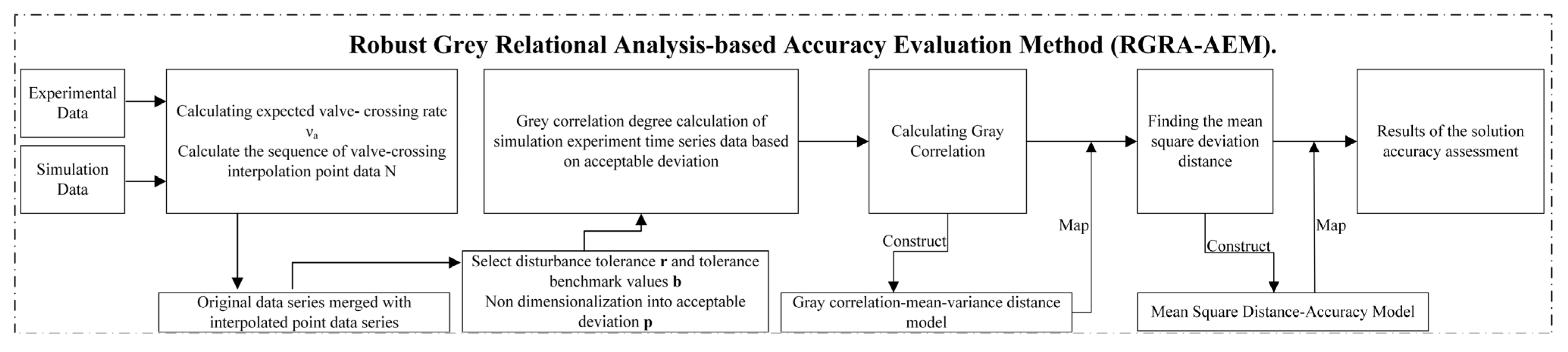
3. Robust Grey Relational Analysis-Based Accuracy Evaluation Method

The essence of traditional grey relational analysis (GRA) lies in evaluating the similarity of the spatial curves formed by time series data based on the distances between corresponding data points. However, this method has a fundamental issue: it does not consider the relative distances between the two sequences, leading to inaccuracies in the evaluation of sequence correlation. As illustrated in the case shown in Figure 2, where $X_0$, $X_1$, $X_2$, and $X_3$ represent different data sequences, the traditional GRA method exhibits the following problems:

(1)

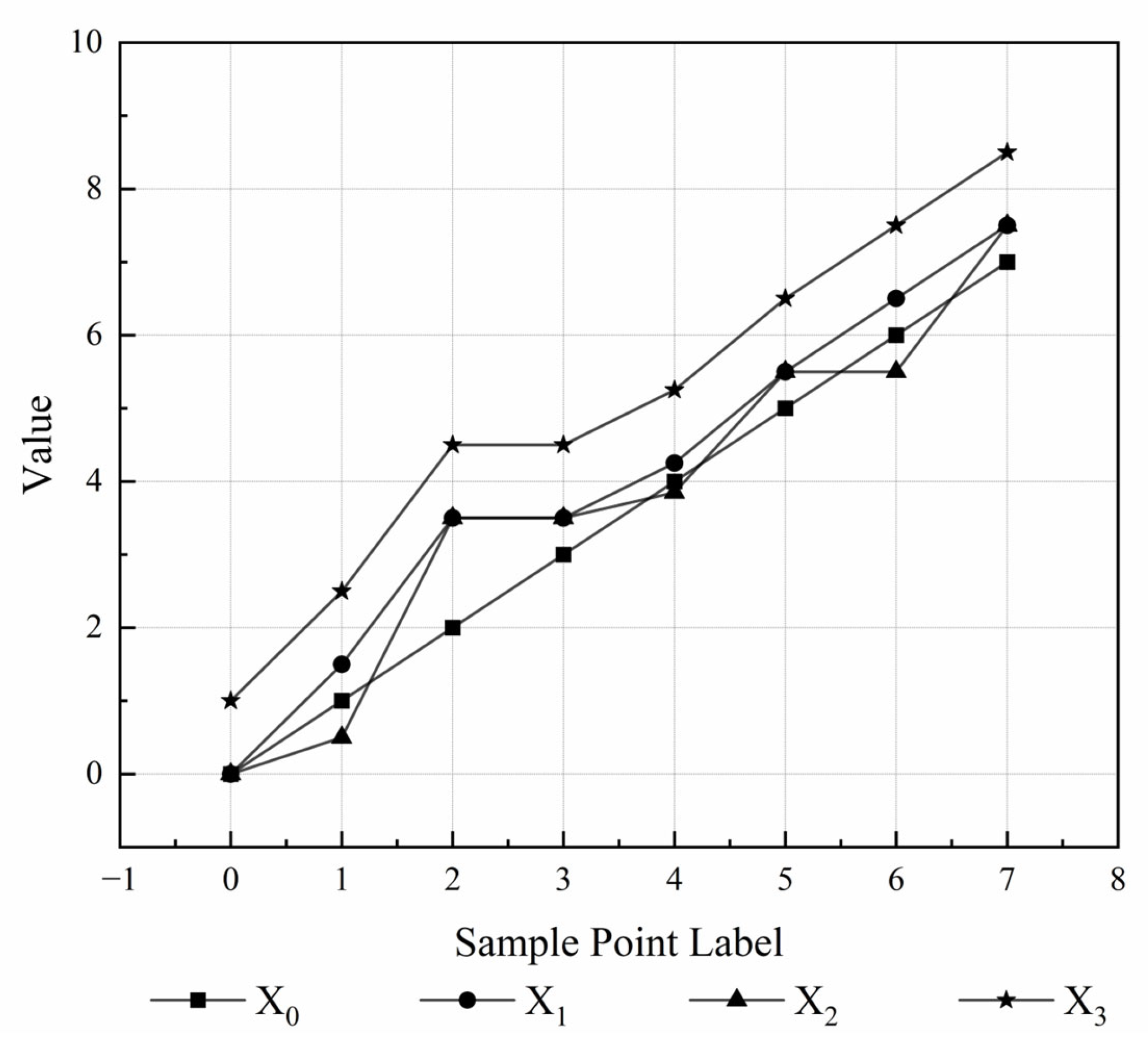
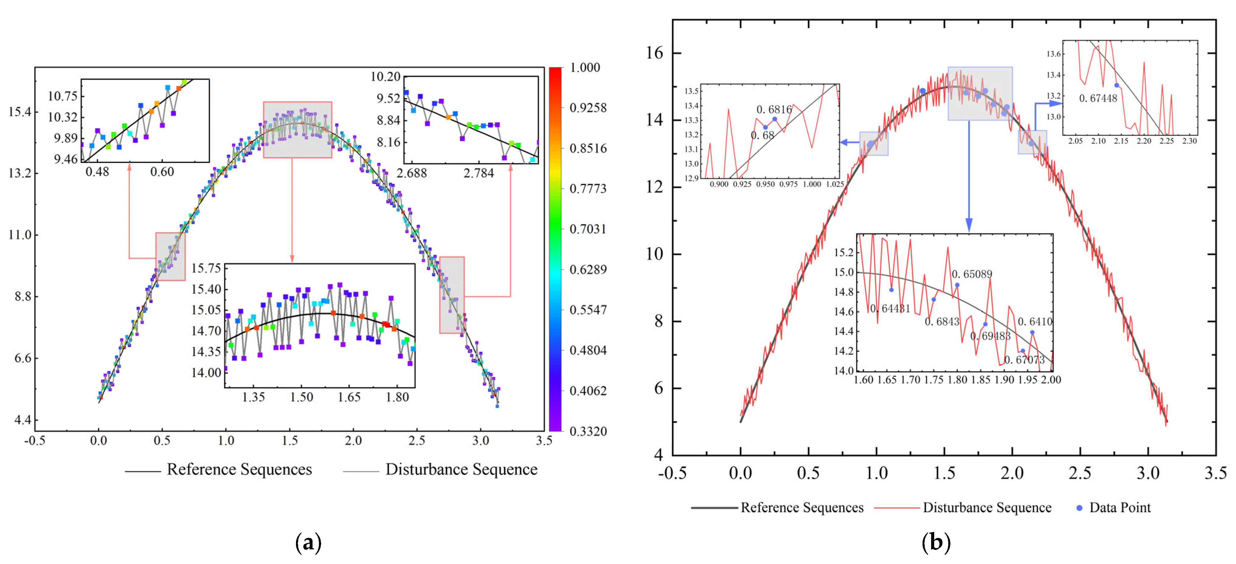
Intuitively, when comparing the consistency of sequences $X_1$ and $X_2$ with sequence $X_0$, it can be observed that sequence $X_2$ should exhibit better consistency with $X_0$ than with $X_1$. This leads to $\gamma (X_0,X_1)<\gamma (X_0,X_2)$. However, in the case where the differences between the data points of sequences $X_1$ and $X_2$ and the reference sequence $X_0$ are equal or opposite values, the traditional grey relational analysis (GRA) yields $\gamma (X_0,X_1)=\gamma (X_0,X_2)$, which contradicts the actual observation.

(2)

For sequences $X_1$ and $X_3$ that exhibit a parallel trend, where the displacement difference at each sampling point is a constant, the minimum differences $\underset{k}{\min }\left|X_1(k)-X_3(k)\right|$ and maximum differences $\underset{k}{\max }\left|X_1(k)-X_3(k)\right|$ between the two sequences are equal. In this scenario, the traditional grey relational analysis (GRA) method yields $\gamma (X_1,X_3)=1$, which fails to account for the relative distances between the sequences, leading to a result that does not align with the actual observations.

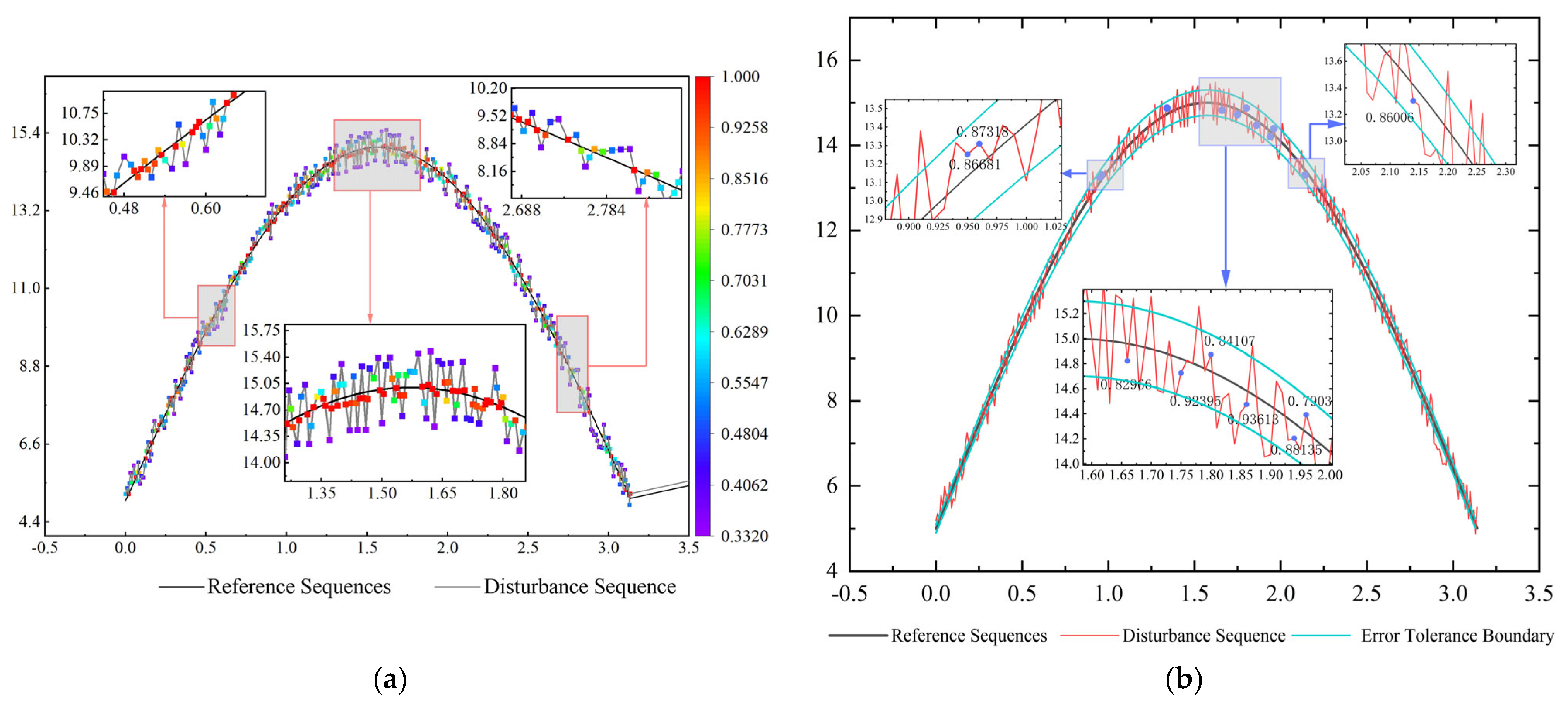
(3)

There are cases where the data points of the sequences are relatively close to each other; however, due to the significant difference in the range (the difference between the maximum and minimum values) of the sequences, the grey relational coefficient is low, which, in turn, results in a low overall grey relational degree.

In this paper, we address the first issue by introducing the expected valve crossing rate combined with an interpolation function to calculate the corrected distance points of the sequences. This approach increases the weight of the grey relational coefficient in the valve crossing point domain. For the second and third issues, we propose a bias tolerance control index to filter and screen time series data, assess the proximity of data sequences, and construct a distance weighting function. This function corrects the distances and geometric shapes of time series data on a small scale to enhance the robustness of the grey relational degree evaluation results. We combine the grey relational degree, mean square deviation distance, and accuracy model to achieve accuracy evaluation, and propose a robust grey relational analysis-based accuracy evaluation method (RGRA-AEM).

3.1. Expected Valve Crossing Rate

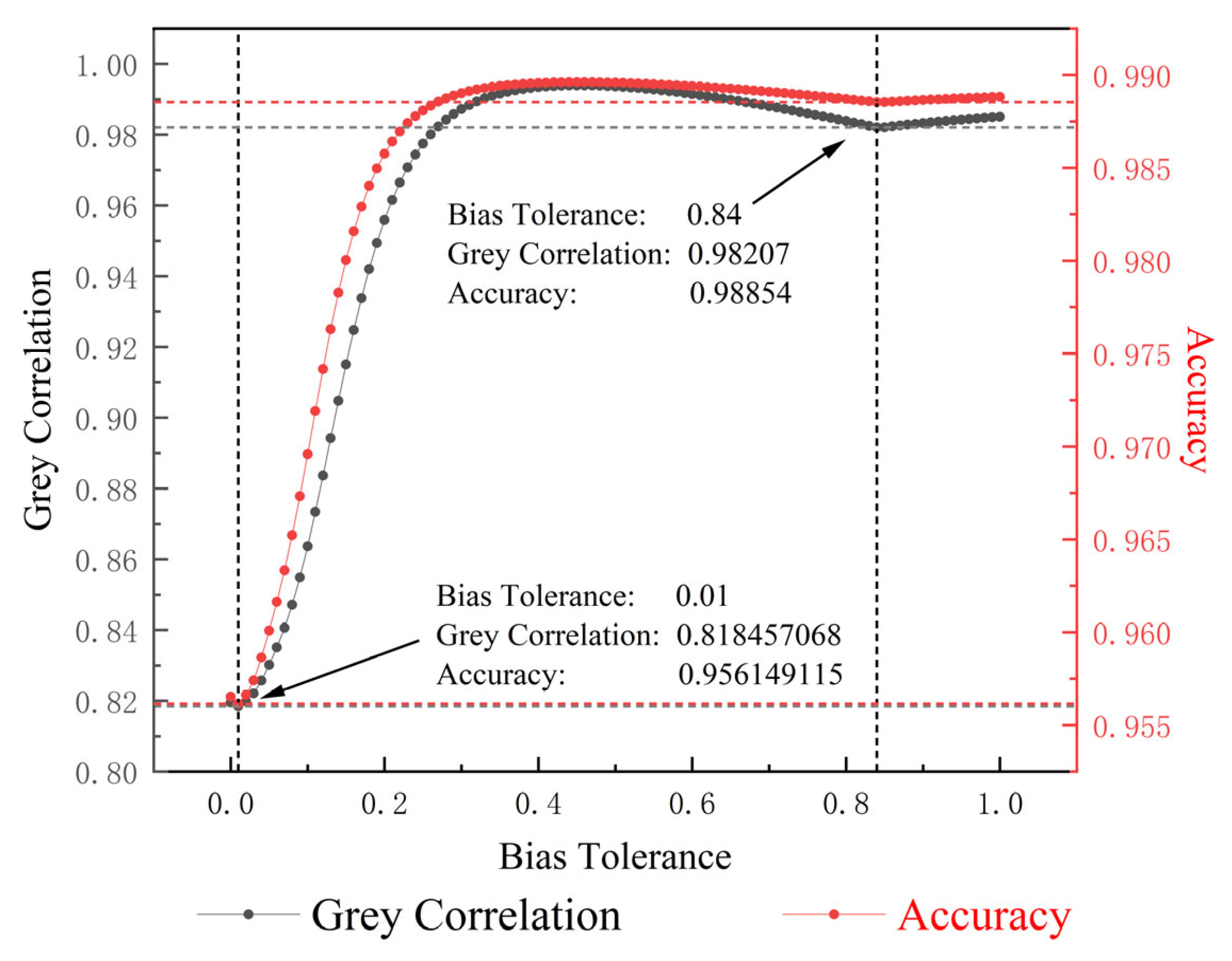
The expected through-the-valve rate was originally proposed by Rice in 1944 as a secondary statistic for describing stochastic processes and their envelopes, and a mathematically more perfect derivation was subsequently given by Middleton [29] in 1960. In this paper, the expected through-the-valve rate is employed to determine the frequency at which the perturbed sequence’s spatial curve intersects the reference sequence as well as the through-the-valve point neighborhood spatial position ranges, which provide positional references for the subsequent construction of interpolation points.

Let $Y\left(t\right)$ be a random sequence of consecutive states at consecutive times and at least once squarely differentiable; then, the number of times the sequence $Y\left(t\right)$ traverses the valve $a$ in the time $\left[t_1,t_2\right]$ is said to be the number of times it penetrates the valve, and its expectation can be constructed with the help of the unit step function $u$ as a 0–1 process function $Z\left(t\right)$:

$$Z(t)=u[Y(t)-a]$$

(7)

here, $u$ is the unit step function, and $a$ is the valve value.

The formal derivative of $Z\left(t\right)$ is as follows:

$$\dot{Z}(t)=\dot{Y}(t)\delta [Y(t)-a]$$

(8)

here, $\delta$ is the Dirac function.

Then, the number of times $N_a(t_1,t_2)$ the random sequence $Y\left(t\right)$ traverses the valve a in the time interval $\left[t_1,t_2\right]$ is as follows:

$$N_a(t_1,t_2)={\displaystyle {\int }_{t_1}^{t_2}\left|\dot{Y}(t)\right|\delta \left[Y(t)-a\right]dt}$$

(9)

The expected number of valve penetrations is as follows:

$$\begin{array}{cc}E[N_a(t_1,t_2)]& ={\displaystyle {\int }_{t_1}^{t_2}E\left[\left|\dot{Y}(t)\right|\delta \left[Y(t)-a\right]\right]dt}\hfill \\ & ={\displaystyle {\int }_{t_1}^{t_2}{\displaystyle {\int }_{-\infty }^{+\infty }{\displaystyle {\int }_{-\infty }^{+\infty }\left|\dot{y}\right|\delta (y-1)p(y,\dot{y},t)dyd\dot{y}dt}}}\hfill \\ & ={\displaystyle {\int }_{t_1}^{t_2}{\displaystyle {\int }_{-\infty }^{+\infty }\left|\dot{y}\right|p(a,\dot{y},t)d\dot{y}dt}}\hfill \end{array}$$

(10)

The number of desired valve penetrations per unit time, i.e., the desired valve penetration rate, is as follows:

$${\upsilon }_a={\displaystyle {\int }_{-\infty }^{+\infty } \left|y\right| p(a,\dot{y},t)d\dot{y}}$$

(11)

The higher the expected through the valve rate, proving that the perturbed sequence curve traverses the reference sequence curve more times per unit of time, the smaller the distance between the relative positions of the perturbed sequence and the reference sequence within the range of a certain perturbation threshold through the valve point. The grey correlation should be given to positive gain, such as in the reference example in Figure 2, where the X₁ and X₂ curves are in the range of the definition, ${\upsilon }_a(X_1)<{\upsilon }_a(X_2)$; however, the results of the calculation of the grey correlation of the data points 1 and 2 are $\gamma (X_0,X_1)=\gamma (X_0,X_2)$.

Therefore, it is possible to indirectly increase the weight of the influence of distance on the gray correlation by increasing the number of computed data points in the neighborhood of the penetrating valve point. In order to ensure that the spatial shape of the curve composed of the data sequence does not change, as well as to avoid the impact of the size of the local extreme difference in the neighborhood of the penetrating valve point on the distribution of the inserted data points, the creation of the data points is carried out using the unilinear interpolation, bilinear interpolation, or trilinear interpolation according to the different dimensions of the data.

The arithmetic example shown in Figure 3 is validated using the Gramacy and Lee Function [30] as the basis function, as follows:

$$f(x)={\displaystyle \frac{\sin (10\pi x)}{2x}}+{(x-1)}^4$$

(12)

here, $f$ denote the Gramacy and Lee Function, and $x$ is the independent variable, which is usually evaluated on the domain $\left[0.5,2.5\right]$.

On the basis of this function, to add a random perturbation to construct the perturbed sequence data, sequence one is the result of a random perturbation under positively proportional weighting coefficients. The reference sequence and the corresponding data point difference of sequence one are used as the benchmark, using a random ± 1 times the gain to construct sequence two, to satisfy sequences one and two in the corresponding data point, and the difference between the reference sequence is equal or opposite.

Grey correlation is calculated for the two sets of sequence data. The results are shown in

Table 1. Comparison of evaluation results between two grey relational analysis methods under equidistant difference conditions.

Statistical Indicators	Traditional Method		RGRA-AEM
	Sequence I	Sequence II	Sequence I	Sequence II
Grey Correlation/(%)	87.3134	87.3134	87.1090	89.7850
Accuracy/(%)	97.1851	97.1851	97.1377	97.7010

, and it is found that, under the traditional grey correlation analysis method, the grey correlation of the two sets of sequence data is equal, which is 87.3134%, and the accuracy after model mapping is 97.1851%, which is not in accordance with the actuality; by judging the expected rate of penetration of the valve of the sequences I and II, respectively, it is obtained that the ${\upsilon }_{a,\mathrm{I}}<{\upsilon }_{a,\mathrm{II}}$. Sequence merging is carried out after calculating the sequence of wearing valve points, respectively, and the merged sequence index is taken to carry out the unilinear difference on the original data sequences I and II, and calculate the grey correlation corresponding to interpolated sequences I and II. The grey correlation of the interpolated sequences I and II is 87.1090% and 89.7850%, respectively, and the accuracy of the sequences after the model mapping is 97.1377% and 97.7010%, respectively. Calculated and verified using the TIC unequal coefficients method, we get ${\mathrm{TIC}}_{\mathrm{I}}=0.12544>{\mathrm{TIC}}_{\mathrm{II}}=0.11904$. That is, the fitting accuracy of sequence II for the reference sequence is greater than that of sequence I, which is consistent with the evaluation results of the improved method in this paper.

The near-identical MAPE–accuracy scores for sequence I and sequence II (75.2848% vs. 75.2869%) reveal critical metric instability that contradicts both the a priori superiority of sequence II and TIC evaluation conclusions. This paradoxical prioritization stems from MAPE’s inherent flaws, exacerbated by the following sequence perturbations: (1) Denominator-induced instability from near-zero actual values amplifies computational sensitivity; (2) Asymmetric error weighting systematically distorts positive/negative deviation impacts; (3) Percentage normalization artificially inflates minor absolute errors into exaggerated deviations in low-magnitude regions. Furthermore, the metric’s sign dependence invalidates mathematical rigor when prediction–actual polarity mismatches occur, while its scale invariance obscures absolute error magnitude—a dual limitation particularly detrimental in zero-rich or volatile datasets. These compounded deficiencies depress accuracy scores below true performance thresholds, ultimately inducing distorted assessments that misrepresent sequence quality under perturbation conditions.

3.2. Bias Tolerance

Figure 4 uses the perturbation sequence constructed by using the sine function as the base function and adding random perturbations as an example. From the figure, it can be seen that when there is a perturbation situation, at a larger geometric scale, the perturbation data sequence and the test data sequence are geometrically similar, and it can be seen that the simulation is acceptable; however, at a smaller geometric scale, the simulation accuracy of the grey correlation analysis is unacceptable. Therefore, in the face of too “harsh” geometric similarity evaluation conditions, qualified models often produce unqualified evaluation results in engineering.

The grey correlation result presented in the figure is about 54.315%, and the accuracy result of its corresponding assessment is only about 68.312%; however, this type of perturbation is perfectly acceptable for practical applications.

The distribution of global grey correlation coefficients in the example is shown in Figure 5a, and the local grey correlation coefficients of the data points are shown in Figure 5b. It was found that, due to the two-level extreme difference being too large as well as the error in the selection of resolution coefficients, the existence of the data points presents a small difference in the distance from the reference series. However, the grey correlation coefficients are small, which, in turn, affects the overall grey correlation degree discrimination.

After using the expected through-the-valve rate to assess the sequence curve through-the-valve situation and linear interpolation, the assessed grey correlation result is about 62.048%, which corresponds to the assessed accuracy result of about 80.504%, which is a certain increase in comparison with the assessment result of the traditional grey correlation analysis method; however, as shown in Figure 6, there still exists a slightly lower assessment result for the data points within the 1% deviation range of the original data.

It can be concluded that the use of the expected through-valve rate to assess the sequence curve and valve situations—combined with linear interpolation for grey correlation analysis—improves the accuracy of the grey correlation results. This improvement comes from increasing the number of interpolation points through the valve to increase the number of evaluation data points in a certain neighborhood of the reference sequence data, so that the grey correlation calculation of the distance weight increases, effectively making up for the traditional grey correlation analysis. To judge the similarity of the sequence curve is to ignore the distance similarity. However, it still belongs to the macro-improvement method, and the optimization object is the data series as a whole, and no improvement is made to the assessment results of single data points.

Therefore, this paper further proposes a quantitative measure of perturbation tolerance $\mathrm{r}=[r_1,r_2,\dots ,r_n]$, $n\in R$ on the basis of the through-valve interpolation method, which means that, for the size of error that a simulation result can be accepted, it is equivalent to adding an error tolerance band. In addition, the simulation results within the error tolerance band are all plausible, and the grey correlation coefficient of a single data point is corrected. After adding the perturbation tolerance index, the original grey correlation analysis method evaluation formula becomes as follows:

$$\begin{array}{l}\gamma (\mathit{X},\mathit{Y})={\displaystyle \frac{1}{n}}{\displaystyle \sum _{i=1}^n\frac{\underset{i}{\min } \underset{k}{\min } |x_i(k)-y_i(k)|+\tau \underset{i}{\max } \underset{k}{\max } |x_i(k)-y_i(k)|}{\left|{\delta }_i\right|+\tau \underset{i}{\max } \underset{k}{\max } |x_i(k)-y_i(k)|}}\\ s.t.\hspace{1em}\hspace{1em}\hspace{1em}{\delta }_i=\left\{\begin{array}{cc}{x}_i(k)-y_i(k)\hfill & if \left|x_i(k)-y_i(k)\right|\ge r_i\hfill \\ f(z_i,r_i)\left[x_i(k)-y_i(k)\right]& if \left|x_i(k)-y_i(k)\right|<r_i\hfill \end{array}\right.\end{array}$$

(13)

where $f(z_i,r_{\mathrm{i}})$ is a weight function that is satisfied as follows:

$$\left\{\begin{array}{l}\underset{z_i\to 0}{\lim }f(z_i,r_i)=0\\ \underset{z_i\to r_i}{\lim }f(z_i,r_i)=1\\ z_i=\left|x_i-y_i\right|\end{array}\right.$$

(14)

In this paper, the Sigmoid function is used as the basis, and Equation (14) is the boundary condition for function fitting to achieve a small slope and a smooth transformation near the boundary of the error tolerance band, which is used to construct an S-shaped distribution of the weights, so that the outputs are restricted to a specific range, which is conducive to the stability and explanatory nature of the model’s weight update.

Using the experimental time series data as the reference sequence b, the disturbance tolerance dimensionless parameter of deviation acceptability p satisfies Equation (15):

$$\mathrm{r}=\mathrm{p}\times \mathrm{b}$$

(15)

The grey correlation formula, after adding the fitted weight function, is shown in Equation (16) as follows:

$$\begin{array}{l}\gamma (\mathit{X},\mathit{Y})={\displaystyle \frac{1}{n}}{\displaystyle \sum _{i=1}^n\frac{\underset{i}{\min } \underset{k}{\min } | x_i(k)-y_i(k)|+\tau \underset{i}{\max } \underset{k}{\max } | x_i(k)-y_i(k)|}{\left|{\delta }_i\right|+\tau \underset{i}{\max } \underset{k}{\max } | x_i(k)-y_i(k)|}}\\ s.t.\hspace{1em}\hspace{1em}\hspace{1em}{\delta }_i=\left\{\begin{array}{cc}{x}_i(k)-y_i(k)\hfill & if {\displaystyle \frac{\left|x_i(k)-y_i(k)\right|}{\mathrm{b}}}\ge \mathrm{p}\hfill \\ {\displaystyle \frac{x_i(k)-y_i(k)}{1+\exp \left[3\ln 10\times (1-\frac{2}{r_i}{z}_i)\right]}}& if {\displaystyle \frac{\left|x_i(k)-y_i(k)\right|}{\mathrm{b}}}<\mathrm{p}\hfill \end{array}\right.\end{array}$$

(16)

where $z_i=\left|x_i-y_i\right|$.

In summary, we optimize the grey correlation coefficients at each point of the data series by using (100 ± p)% times the benchmark value as the error tolerance boundaries for different cases corresponding to the appropriate p-value and optimize the grey correlation coefficients at each point of the data series by combining the linear difference method after the discrimination of the expected through-valve rate, so as to construct the accuracy assessment method based on the strong robust grey correlation analysis.

The through-valve interpolation method corrects the grey correlation equation for distance weights, and the bias acceptability metric is filtered for grey correlation coefficients. A global average deviation of 2% was used as the selection criterion for deviation acceptability for the example in Figure 4. The grey correlation coefficients of data points with 2% deviation acceptability added after using through-valve interpolation are shown in Figure 7, and the calculation results are shown in

Table 2. Comparison of evaluation results between two grey relational analysis methods under disturbance conditions.

Statistical Indicators	Traditional Method	RGRA-AEM
	No Additional Interpolation Points Through the Valve	No Additional Interpolation Points Through the Valve	Increase Penetration Valve Interpolation Points
	No Increase in Bias Tolerance	Increase in Bias Tolerance by 2%	No Increase in Bias Tolerance	Increase in Bias Tolerance by 2%
Grey Correlation/(%)	54.315	58.0955	62.048	68.439
Accuracy/(%)	68.312	74.760	80.504	87.602

. Through a comparison of Figure 7a and Figure 5a, it is found that the use of this paper’s method increases the grey correlation coefficient of each data point within a certain deviation range of the reference sequence. This strengthens the weight coefficient of the distance when calculating the grey correlation coefficient, which is obtained by calculating the TIC inequality coefficient $TIC=0.01032$, which proves that the fitting accuracy of the sequence is higher; in the case using both the through-valve interpolation method and bias acceptability, the overall grey correlation degree of the sequence reaches 68.439%, and the accuracy reaches 87.602%. Compared with the traditional grey correlation analysis method, the method suggested in this paper is more in line with the TIC discrimination conclusion.

3.3. Accuracy Assessment Process Based on Strong Robust Grey Correlation Analysis

The accuracy assessment steps based on strong robust grey correlation analysis are summarized as shown in Figure 8. Firstly, calculate the expected through-valve rate and the through-valve interpolation point data sequence, merge the interpolation point sequence with the original data sequence, select the perturbation tolerance and tolerance benchmark sequence according to the actual engineering application, dimensionless them to the bias acceptability, and construct the grey correlation coefficient–mean squared distance model and the mean squared distance–accuracy model based on the time series data from the simulation and test. Based on the simulation-test time series data, the grey correlation coefficient and grey correlation degree are calculated based on the acceptable deviation, and the grey correlation degree is mapped to the mean square distance by combining the grey correlation degree–mean square distance model. The mean square distance is mapped to the accuracy assessment result by combining the mean square distance–accuracy model.

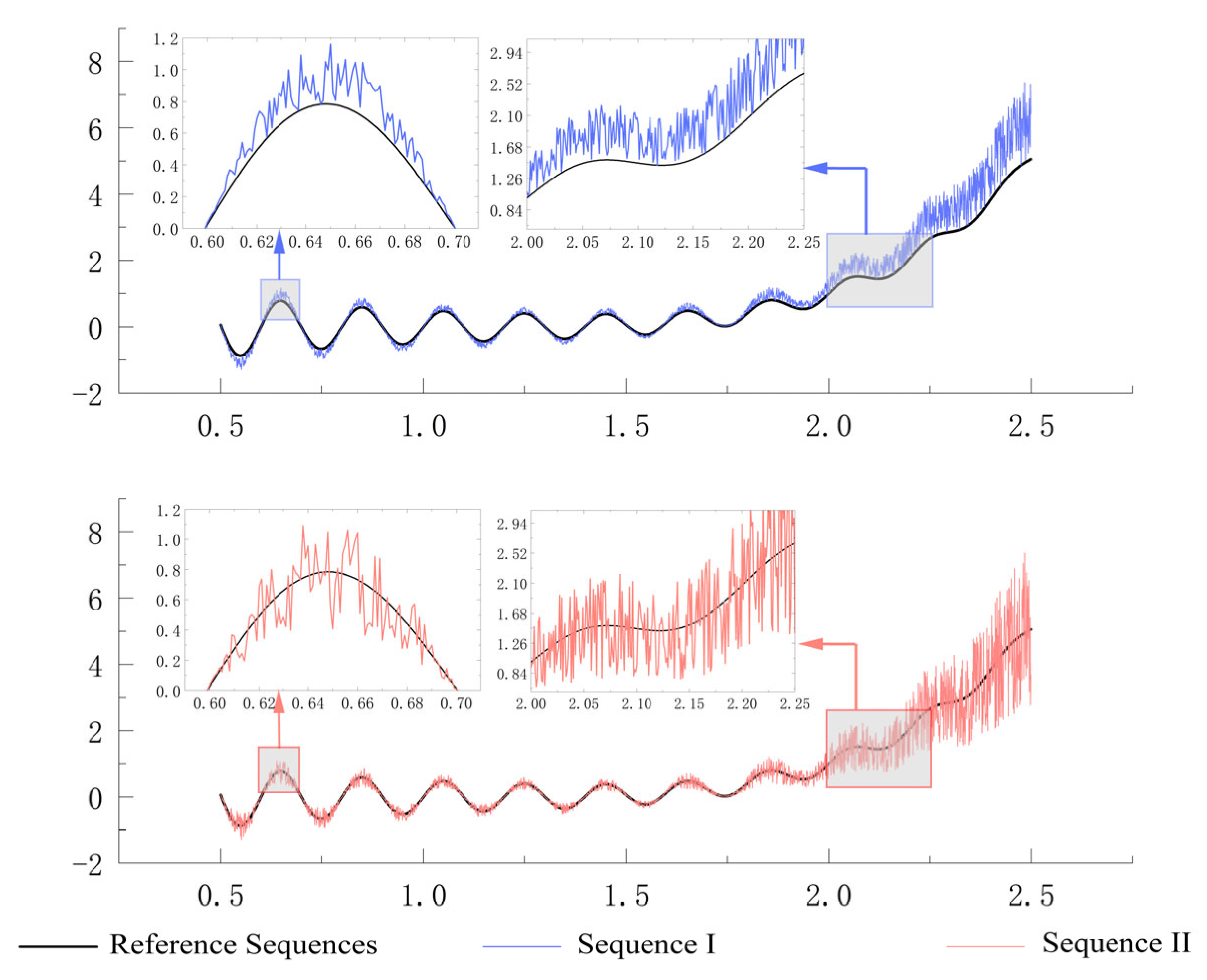
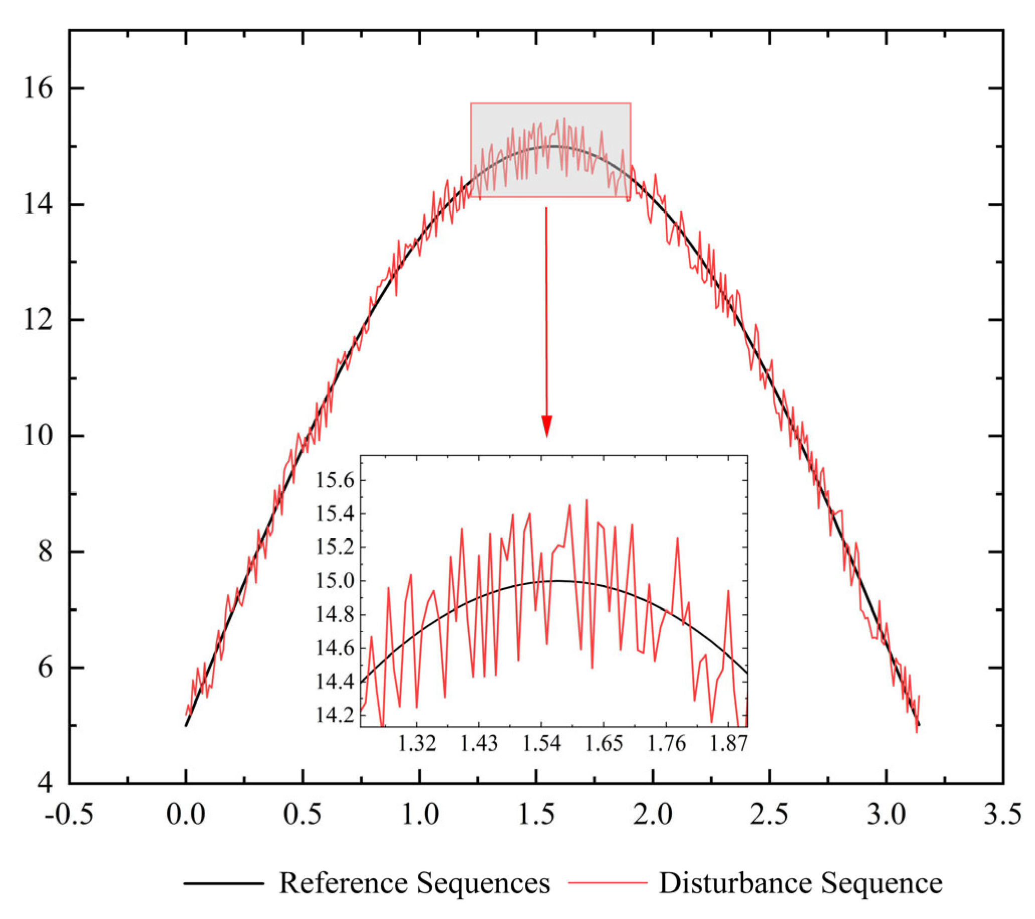
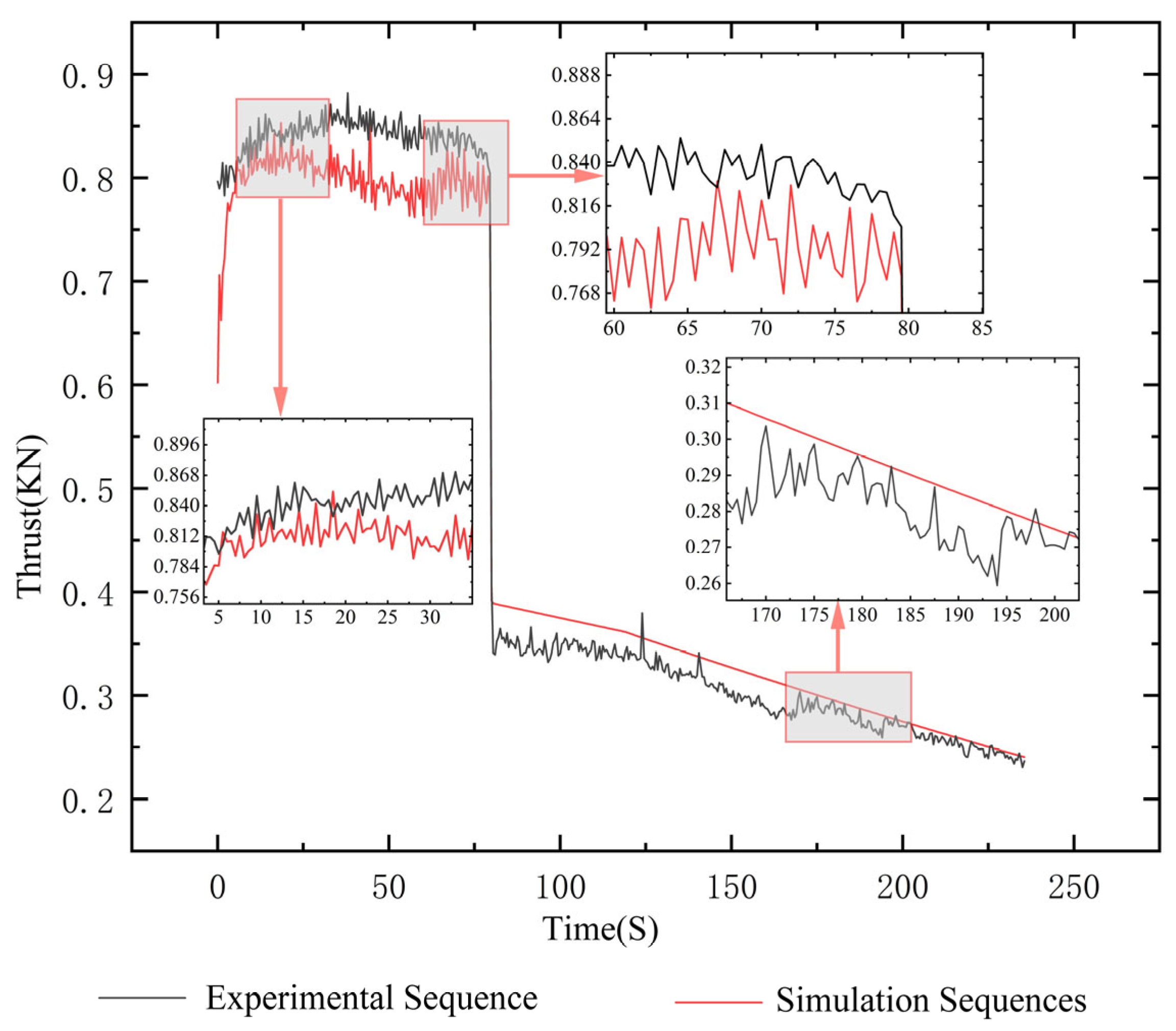
4. Instance Validation

In order to verify the improvement effect and practical application of the proposed method in Section 3, we carried out an example verification on a hybrid rocket motor. The hybrid rocket motor uses a solid fuel of hydroterminated polybutadiene (HTPB) and a liquid oxidizer of hydrogen peroxide (H₂O₂), with the return and specific impulse of the fuel improved by the addition of metal particles.

An accuracy assessment method based on strong robust grey correlation analysis is applied for the internal ballistic test-simulation model validation of a certain type of hybrid rocket motor to analyze the consistency between the output timing data of the model thrust characteristics and that of the actual test [31,32,33].

The timing curves, composed of the experimental sequence and the simulation sequence, are shown in Figure 9, and the two sets of sequence curves have the same trend of change and the same perturbation, which belong to the simulation model with higher accuracy and more reasonable data in engineering applications. The test is carried out through the TIC inequality coefficient, and $\mathrm{TIC}=0.03170$ is obtained.

From Figure 10, it can be concluded that there is a positive correlation between grey correlation and model accuracy; grey correlation and accuracy change curves are similar. As a measure of the similarity between the model output and the actual data, an increase in the grey correlation usually predicts an increase in the model accuracy, i.e., when the correlation between the output of the simulation model and the actual observed data is enhanced, the prediction accuracy of the model tends to improve, which is in line with the nature of the linear mapping of the grey correlation–mean squared deviation distance–accuracy model. As the bias acceptability increases, there is a tendency for the grey correlation and accuracy to first decrease and then increase within a certain tolerance. The perturbation tolerance allows the grey correlation to correct the accuracy bias due to geometric similarity and distance proximity when quantifying the data series curves. In addition, the increase in bias acceptability reflects a greater tolerance for model prediction errors by the user or decision-maker, which may result in higher ratings of model accuracy during the evaluation process, thus increasing the acceptance of the model’s accuracy overall.

The selection criterion of bias acceptability for this example is based on the global average deviation of 5%. The relative position of the data series curve with the 5% bias acceptability added after interpolation using the through-valve is shown in Figure 11 in relation to the error tolerance boundary.

Figure 12a shows the distribution of grey correlation coefficient using the traditional grey correlation analysis method, corresponding to the grey correlation degree of 80.4016% and accuracy of 95.0768% in

Table 3. Comparison of evaluation results between two grey relational analysis methods.

Statistical Indicators	Traditional Method	→		RGRA-AEM
	No Additional Interpolation Points Through the Valve	Only Increase Penetration Valve Interpolation Points	Only Increase in Bias Tolerance by 5%	Increase Penetration Valve Interpolation Points
	No Increase in Bias Tolerance			Increase in Bias Tolerance by 5%
Total number of positions	472	589	472	598
Number of data points corrected	0	126	200	326
Grey Correlation/(%)	80.4016	81.8313	81.3763	83.0590
Accuracy/(%)	95.0768	95.6098	95.4465	96.0231

; Figure 12b shows the distribution of grey correlation coefficient by using only valve interpolation, corresponding to the grey correlation degree of 81.8313% and accuracy of 95.6098%; comparing Figure 12a with Figure 12b, it is found that the essence of valve interpolation lies in increasing the number of data points within the proximity range of the sequence curve without changing the shape of the original sequence curve in order to indirectly increase the proportion of distance proximity in the calculation of the grey correlation coefficient. Moreover, due to the increase in the fitting accuracy caused by the increase in the number of data points, the corresponding TIC coefficients will also change accordingly: ${\mathrm{TIC}}_{\mathrm{a}}=0.03170>{\mathrm{TIC}}_{\mathrm{b}}=0.03107$.

Figure 12c shows the distribution of grey correlation coefficients under the use of bias acceptability only, which corresponds to a grey correlation of 81.3763% and an accuracy of 95.4465%; comparing Figure 12a with Figure 12c, it can be found that the essence of bias acceptability lies in the correction of grey correlation coefficients of the data points in the tolerance band of error, which acts directly on the data points in the tolerance band and does not change the original data distribution as well as the fitting accuracy, as follows: ${\mathrm{TIC}}_{\mathrm{a}}=0.03170={\mathrm{TIC}}_{\mathrm{c}}=0.03170$.

Figure 12d shows the distribution of grey correlation coefficients after the combined use of through-valve interpolation as well as bias acceptability, at which point the grey correlation is 83.0590% and the accuracy is 96.0231%.

By correcting the grey correlation coefficients of individual data points in the microscopic level and selectively increasing the sequence data points in the macroscopic level to indirectly enhance the distance weights, a robust grey correlation analysis method is constructed; when dealing with perturbed time series datasets and noisy data, the new method shows higher stability and reliability, and it can better take into account the uncertainties of perturbation in a small-scale range or the complexity of the noise in the practical application scenarios. The robustness of the grey correlation analysis model is improved.

5. Conclusions

In this paper, in response to the phenomenon of the poor robustness of grey correlation analysis method in dealing with the accuracy assessment of noisy data, the interpolation method guided by the expected penetration rate is introduced, and on the basis of not changing the shape of the curve of the original data series, the weight of the data distance for the calculation of the grey correlation analysis is indirectly increased by increasing the number of data points within the range of the difference of the distance of a small distance, and the indicator of the acceptable degree of bias p is proposed to be the threshold of the distance of the data. On the basis of taking the absolute value of the difference in the grey correlation analysis interpolation, the weight correction after judging the tolerance of perturbation is added, and the grey correlation is mapped to the accuracy by constructing the grey correlation–mean square, distance–accuracy model. The grey correlation coefficient of individual data points is corrected in the microcosm, and the weight of the data point distance is increased in the macrocosm, which effectively improves the anti-noise performance and anti-perturbation performance of the evaluation results and helps to accurately and clearly reflect the accuracy of the simulation model. This method may have potential applications in many more areas, such as neural network modeling, quality assessment for time series data, and assisted assessment of calibration quality for multi-sensor data alignment calibrations. In future research, we wanted to optimize these methods from a more data-driven perspective. It is an important to select a more reasonable hyperparameter (e.g., the acceptable degree of bias p) that is less disturbed by human factors.

References

1. Deng, J.; Zhou, C. Sufficient condition for stability of grey systems and its application in the analysis of stability of linear time-varying systems. Inf. Control 1987, 4, 24–27. [Google Scholar]
2. Deng, J. Introduction to gray system theory. Inn. Mong. Power 1993, 3, 51–52. (In Chinese) [Google Scholar]
3. Tian, M.; Liu, S.; Bu, Z. A review of research on grey correlation algorithm modeling. Stat. Decis.-Mak. 2008, 1, 24–27. (In Chinese) [Google Scholar]
4. Zhou, W.; Zeng, B. A research review of grey relational degree model. Stat. Decis. 2020, 36, 29–34. [Google Scholar]
5. Wei, H.; Li, Z. Grey relational analysis and its application to the validation of computer simulation models for missile systems. Syst. Eng. Electron. 1997, 2, 55–61. [Google Scholar]
6. Ning, X.; Wu, Y.; Chen, Z. Study on validation of simulation models based on improved grey relational analysis. Comput. Simul. 2015, 32, 259–263. [Google Scholar]
7. Ning, X.; Wu, Y.; Yu, T.; Chen, W.; Shan, B.; Zhang, Y. Research on comprehensive validation of simulation models based on improved grey relational analysis. Acta Armamentarii 2016, 37, 338–347. [Google Scholar]
8. Wu, J.; Wu, X.; Chen, Y.; Teng, J. Validation of simulation models based on improved grey relational analysis. Syst. Eng. Electron. 2010, 32, 1677–1679. [Google Scholar]
9. Zhang, Y.; Shang, K. Evaluation of mine ecological environment based on fuzzy hierarchical analysis and grey relational degree. Environ. Res. 2024, 257, 119370. [Google Scholar] [CrossRef]
10. Mei, Z. The concept and computation method of grey absolute correlation degree. Syst. Eng. 1992, 5, 43–44+72. [Google Scholar]
11. Tang, W. Some shortcomings of grey absolute correlation degree. J. Syst. Eng. 1994, 5, 59–62. [Google Scholar]
12. Tang, W. The concept and the computation method of t’s correlation degree. J. Appl. Stat. Manag. 1995, 1, 34–37+33. [Google Scholar]
13. Shen, M.; Hu, B. The modified t’s correlative degree and its application in the securities business. Syst. Eng. Theory Pract. 2003, 5, 36–40. [Google Scholar]
14. Prakash, J.U.; Sivaprakasam, P.; Juliyana, S.J.; Ananth, C.; Rubi, C.S.; Sadhana, A.D. Multi-objective optimization using grey relational analysis for wire EDM of aluminium matrix composites. Mater. Today Proc. 2023, 72, 2395–2401. [Google Scholar] [CrossRef]
15. Ben Taher, M.A.; Pelay, U.; Russeil, S.; Bougeard, D. A novel design to optimize the optical performances of parabolic trough collector using Taguchi, ANOVA and grey relational analysis methods. Renew. Energy 2023, 216, 119105. [Google Scholar] [CrossRef]
16. Zhang, M.; Zhao, H.; Fan, L.; Yi, J.; Junyan, Y. Dynamic modulus prediction model and analysis of factors influencing asphalt mixtures using gray relational analysis methods. J. Mater. Res. Technol. 2022, 19, 1312–1321. [Google Scholar] [CrossRef]
17. Gao, S.; Zhi, Y.; Zhang, P.; Zuo, X. Consistency validation method of simulation results based on improved grey relational analysis for aerospace product performance prototype. Syst. Eng. Electron. 2023, 45, 2777–2783. [Google Scholar]
18. Liu, Z.; Xie, Y.; Dang, Y. Characteristic test method of matrix grey incidence degree and its application. Oper. Res. Manag. Sci. 2020, 29, 131–138. [Google Scholar]
19. Hu, A.; Xie, N. Construction and application of a novel grey relational analysis model considering factor coupling relationship. Grey Syst. Theory Appl. 2025, 15, 1–20. [Google Scholar] [CrossRef]
20. Wang, R.; Xu, Y.; Yang, Q. A new adaptive grey seasonal model for time series forecasting tasks. Grey Syst. Theory Appl. 2024, 14, 360–373. [Google Scholar] [CrossRef]
21. Li, X. Research on the computation model of grey interconnet degree. Syst. Eng. 1995, 6, 58–61. [Google Scholar]
22. Liu, S.; Cai, H.; Ying, Y.; Yang, Y. Advance in grey incidence analysis modeling. Syst. Eng.-Theory Pract. 2013, 33, 2041–2046. [Google Scholar]
23. Nowak, M.; Pawłowska-Nowak, M.; Kokocińska, M.; Kułyk, P. The evaluation of grey relative incidence. Grey Syst. Theory Appl. 2024, 14, 263–282. [Google Scholar] [CrossRef]
24. Zhang, L.; Ma, X.; He, Q.; Li, T. A novel unbiased multi-variable grey model. Grey Syst. Theory Appl. 2025, 15, 209–238. [Google Scholar] [CrossRef]
25. Lu, F. Research on the identification coefficient of relational grade for grey system. Syst. Eng.-Theory Pract. 1997, 6, 50–55. [Google Scholar]
26. Sun, Y. Research on Grey Incidence Analysis and Its Application; Nanjing University of Aeronautics and Astronautics: Nanjing, China, 2009. [Google Scholar]
27. Li, Y. Research on Simulation Model Validation Methods and Assistant Tool Based on Grey Relational Analysis; Harbin Institute of Technology: Harbin, China, 2015. [Google Scholar]
28. Zhou, Y. Research on Validation Method for Complex Simulation Model; Harbin Institute of Technology: Harbin, China, 2019. [Google Scholar]
29. Middleton, D. An Introduction to Statistical Communication Theory; McGrawHill: New York, NY, USA, 1960. [Google Scholar]
30. Gramacy, R.B.; Lee, H.K. Cases for the nugget in modeling computer experiments. Stat. Comput. 2012, 22, 713–722. [Google Scholar] [CrossRef]
31. Tan, G.; Tian, H.; Wang, Z.; Guo, Z.; Gao, J.; Zhang, Y.; Cai, G. Experimental investigation into closed-loop control for htpb-based hybrid rocket motors. Aerospace 2023, 10, 421. [Google Scholar] [CrossRef]
32. Tian, H.; Meng, X.; Zhu, H.; Li, C.; He, L.; Cai, G. Dynamic numerical simulation of hybrid rocket motor with htpb-based fuel with 58% aluminum additives. Aerospace 2022, 9, 727. [Google Scholar] [CrossRef]
33. Meng, X.; Tian, H.; Niu, X.; Zhu, H.; Gao, J.; Cai, G. Long-duration dynamic numerical simulation of combustion and flow in hybrid rocket motors considering nozzle erosion. Aerospace 2024, 11, 318. [Google Scholar] [CrossRef]
Figure 1. Grey correlation–mean square distance–accuracy conversion model.
Applsci 15 04926 g001
Figure 2. Reference example.
Applsci 15 04926 g002
Figure 3. Gramacy and Lee function and random data series comparison.
Applsci 15 04926 g003
Figure 4. Schematic diagram of the perturbation data.
Applsci 15 04926 g004
Figure 5. Grey relational coefficients of data points using traditional grey relational analysis: (a) Global distribution of grey relational coefficients, which shows the distribution of gray correlation coefficients for the sequence as a whole; (b) Some sample points with anomalous grey correlation coefficients, highlighting some of the anomalies with small gray correlation coefficients (color blocks represent sample points and their corresponding grey correlation coefficients).
Applsci 15 04926 g005
Figure 6. Grey relational coefficients of local data points after linear interpolation.
Applsci 15 04926 g006
Figure 7. Grey relational coefficients of data points after adding 2% deviation acceptability: (a) Global distribution of grey relational coefficients, which shows the distribution of gray correlation coefficients for the sequence as a whole; (b) Some sample points with anomalous grey correlation coefficients, highlighting some of the anomalies with small gray correlation coefficients. Color blocks represent sample points and their corresponding grey correlation coefficients.
Applsci 15 04926 g007
Figure 8. Methodology flowchart.
Applsci 15 04926 g008
Figure 9. Internal ballistic experimental-simulation thrust time series data of a hybrid rocket engine.
Applsci 15 04926 g009
Figure 10. Grey correlation–accuracy deviation acceptability variation curve.
Applsci 15 04926 g010
Figure 11. Illustration of data at 5% deviation acceptability.
Applsci 15 04926 g011
Figure 12. Grey relational coefficient distribution map of hybrid rocket engine internal ballistic experiment-simulation data: (a) Traditional grey relational analysis, which shows the distribution of gray correlation coefficients under the traditional approach; (b) Interpolation method, highlighting changes in the number of sample points for gray correlation coefficient calculations; (c) Deviation acceptability, highlighting changes in gray correlation coefficients; (d) Robust grey relational analysis, highlighting an overall increase in the correlation coefficient. Color blocks represent sample points and their corresponding grey correlation coefficients.
Applsci 15 04926 g012aApplsci 15 04926 g012b