Photoacoustic Imaging with a Finite-Size Circular Integrating Detector

Abstract

Photoacoustic imaging (PAI) has rapidly developed in biomedical imaging. The point spread function (PSF) is critical for addressing image blurring in PAI. However, in circular integrating detection systems, the PSF exhibits spatial variations. This makes PSF extraction challenging. The existing studies typically assume that the PSF is known or obtained through experiments. This study proposes a method for extracting the PSF based on the polar coordinate system. By transforming the image from the Cartesian coordinate system to the polar coordinate system, the “spin blur” problem is decomposed into multiple independent subproblems. With the separation of the radial and angular directions, the blurring kernel remains invariant at each radius, thereby simplifying the estimation of the PSF. To estimate the blurring kernel, we use polynomial algebraic common factor extraction techniques. The numerical simulation results validate the effectiveness of the method, and the impact of sample size on computational efficiency and accuracy is discussed.

1. Introduction

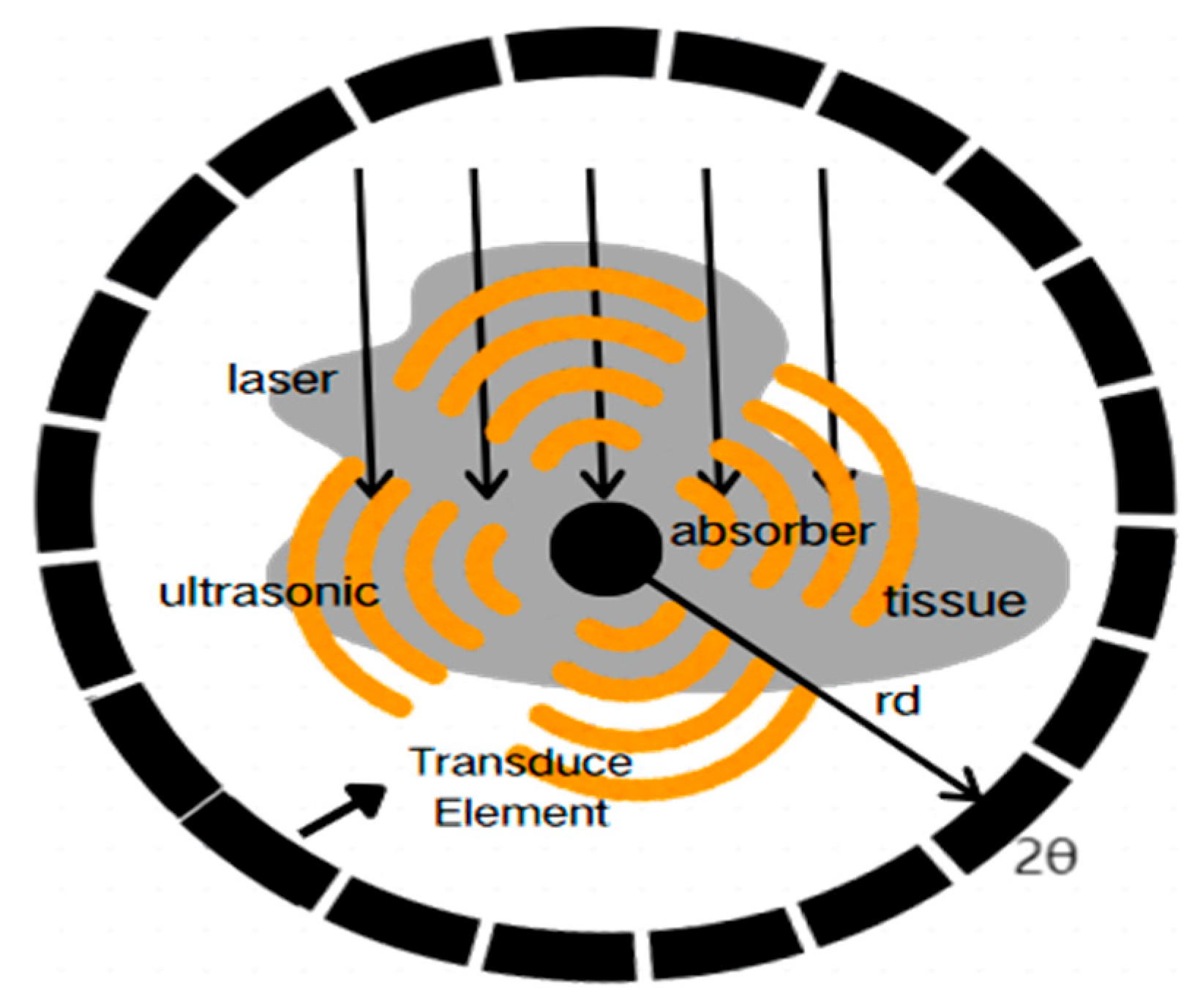
Photoacoustic imaging (PAI) is an emerging biomedical imaging technology that combines the high contrast of optical imaging with the high resolution of ultrasound imaging. PAI uses short-pulse laser excitation on biological tissues. Optically absorbing regions undergo adiabatic expansion, generating ultrasound waves. This phenomenon is known as the photoacoustic effect [1,2]. By detecting the resulting photoacoustic signals, the spatial distribution of optical absorption in biological tissues can be reconstructed. Recent advances in PAI have significantly propelled its clinical translation. PAI enables microvascular oxygenation visualization [3,4] and 3D vasculature reconstruction [5], noninvasive hemodynamic tracking in brain studies [6], and high-resolution cortical mapping [7]. In oncology, PAI is used to monitor tumor neovascularization dynamics [8], and multimodal breast scanners [9], along with molecular characterization [10], improve cancer diagnoses. Sentinel lymph node mapping techniques [11,12,13,14] have further revolutionized surgical navigation. Targeted gold nanorods support theranostics for submillimeter bladder cancer [15], while diversified nanomaterials expand functional imaging capabilities [16]. Despite persistent challenges in in vivo targeting efficiency [17], PAI’s clinical value continues to grow, demonstrating broad potential across medical disciplines.

Ultrasonic detector arrays can be configured in various geometries as a critical component of PAI systems. Circular integrating detectors are compact and symmetric. This design helps to capture accurate structural and functional information about tissues. This ability is particularly valuable in the early diagnosis and precise treatment of breast cancer and in cardiovascular disease assessments [18,19]. However, applying existing image reconstruction algorithms [20,21] that are designed for ideal point detectors to finite-sized circular integrating detectors degrades image reconstruction quality [22].

To mitigate the blurring effects introduced by circular integrating detectors, researchers have proposed the concept of the spatial impulse response (SIR) and developed algorithms to correct the spatial blurring caused by the detectors. Based on a linear and discrete PAI imaging model, Meng Lin Li et al. designed a spatiotemporal optimal filter using the minimum mean square error criterion to correct SIR effects caused by defocused regions, thereby improving tangential resolution [23]. Kenji Mitsuhashi et al. included SIR in their imaging model. They focused on far-field imaging to improve 3D tomography for small animals [24]. Although incorporating SIR into the imaging model enhances imaging accuracy, it also increases computational complexity. To address this issue, Xiao Fei Luo et al. proposed a sensor-based SIR back-projection (BP) method to quickly correct the limitations caused by the detector size, thereby accelerating image reconstruction [25].

The above approach addresses the issue in the data domain before image reconstruction. In the image domain after reconstruction, blind deconvolution methods have become an alternative strategy for handling PAI image blurring. For example, Xianlin Song and Lingfang Song employed a blind deconvolution method to process the reconstructed data to restore PAI images [26]. They employed iterative deconvolution and used focal measurements from a photoacoustic microscope as the initial PSF. They combined their method with Lucy–Richardson (LR) deconvolution. Their method significantly enhanced the vascular imaging resolution. L. Qi et al. developed a spatial variant PSF-based PAI image restoration method. PSF was measured experimentally and estimated with pixel-level precision using multi-Gaussian fitting and interpolation algorithms. Their optimized iterative restoration model substantially enhanced image quality and resolution [27]. Additionally, Wende Dong and colleagues introduced the concept of spatial angular convolution to describe “spin blur”. They constructed a regularized restoration model that further improved image quality using an alternating minimization algorithm [28]. Experimentally measured PSF methods improve imaging quality, but their complexity and costs limit practical applications.

Unlike conventional methods that require either experimental acquisition or prior knowledge to extract the PSF, this study proposes a novel approach that directly extracts blurring kernels from blurred pressure distributions without requiring experimental measurements or any a priori information. By integrating coordinate transformation with polynomial common factor extraction techniques, the proposed method converts rotational blurring problems in Cartesian coordinates into independent deblurring tasks in polar coordinates. Each problem involves pixels at a specific radius, and the pixels at each radius share the same spatially invariant point spread function, i.e., the blurring kernel. To achieve this, we employ a polynomial algebraic common factor extraction technique to further estimate the blurring kernel. Numerical simulations validate the effectiveness of this method, and we discuss the impact of sample quantity on computational efficiency and accuracy. Overall, this method provides an efficient and stable solution to the rotational blur problem in photoacoustic imaging.

2. Methods

2.1. Generation and Propagation of Photoacoustic Waves

A laser pulse irradiates biological tissue, where the absorbers absorb light energy, triggering instantaneous thermal expansion. This results in a pressure increase proportional to the absorbed light energy, generating pressure waves. The general equation for the generation and propagation of PA waves is given by [29]:

$${\displaystyle \frac{{\partial }^{2}p(\mathbf{r},t)}{\partial t^2}}-c^2\mathrm{\Delta }p(\mathbf{r},t)=p_0(\mathbf{r})\cdot {\displaystyle \frac{d}{dt}}\delta (t)$$

(1)

where $p(\mathbf{r},t)$ is the pressure at position $\mathbf{r}$ and time $t$: it describes the pressure signal that is propagating through the medium (such as biological tissue). $p_0(\mathbf{r})$ represents the initial pressure distribution due to thermal expansion, $c$ is the speed of sound in the tissue, and $\delta (t)$ is the Dirac delta function representing the instantaneous excitation.

Equation (1) corresponds to an initial value problem for the homogeneous wave equation:

$${\displaystyle \frac{{\partial }^2}{\partial t^2}}p(\mathbf{r},t)-c^2\mathrm{\Delta }p(\mathbf{r},t)=0$$

(2)

with the initial conditions:

$$p(\mathbf{r},0)=p_0(\mathbf{r}); {\displaystyle \frac{\partial }{\partial t}}p{(\mathbf{r},t)}_{t=0}=0$$

(3)

In PAI, the main goal is to reconstruct the spatial distribution of the sample’s internal energy absorption, which is proportional to the initial pressure distribution $p_0(\mathbf{r})$. To achieve this, the initial pressure distribution $p_0(\mathbf{r})$ needs to be recovered from the pressure signals $p({\mathbf{r}}_{\mathbf{d}},t)$ measured by the detector D on the sample surface S (as shown in Figure 1).

The pressure signal $p(\mathbf{r},t)$ at position $\mathbf{r}$ and time $t$ can be obtained as follows:

$$p(\mathbf{r},t)={\displaystyle \frac{1}{4\pi c}}{\displaystyle {\iint }_{|\mathbf{r}-{\mathbf{r}}^{\prime }|=ct}\frac{p_0({\mathbf{r}}_0)}{|\mathbf{r}-{\mathbf{r}}^{\prime }|}}dS({\mathbf{r}}^{\prime })$$

(4)

In this equation, ${\mathbf{r}}^{\prime }$ represents points on a spherical surface centered around $\mathbf{r}$ with a radius equal to $ct$.

The research in this study is based on the circular integrating detector, and its structure is shown in Figure 2. The finite size of the detector causes it to perform a weighted integral of the acoustic field signal $p(\mathbf{r},t)$ within its sensing region. The recorded signal $p_{\omega }({\mathbf{r}}_{\mathbf{d}},t)$ is essentially the result of the convolution between the SIR ${\omega }_{\det }(r,t)$ and the acoustic field signal $p({\mathbf{r}}_{\mathbf{s}},t)$. The SIR describes the spatial averaging effect of the detector on the received acoustic signal. The mathematical expression for the recorded signal of a finite-size detector can be written as follows [30]:

$$p_{\omega }({\mathbf{r}}_{\mathbf{d}},t)={\displaystyle \underset{S}{\int }{\omega }_{\det }(\left|{\mathbf{r}}_{\mathbf{d}}-{\mathbf{r}}_{\mathbf{s}}\right|,t)}\cdot p({\mathbf{r}}_{\mathbf{s}},t)dS({\mathbf{r}}_{\mathbf{s}})$$

(5)

Here, ${\mathbf{r}}_{\mathbf{d}}$ indicates the center of the detector, while ${\mathbf{r}}_{\mathbf{s}}$ represents positions on the detector’s surface. S is the sensing area of the detector. When we apply reconstruction algorithms designed for ideal point detectors, such as time reversal or backprojection, to $p_{\omega }({\mathbf{r}}_{\mathbf{d}},t)$, the reconstructed image will exhibit blurring.

Figure 2. Schematic diagram of the circular array PAI system.

Figure 2. Schematic diagram of the circular array PAI system.

2.2. Blurring Effects of Circular Integrating Detectors

According to [31], the finite size of the circular integrating detector causes a spatially variant blur. The PSF exhibits spatially variant characteristics. The blurred pressure distribution can be expressed as the convolution of the initial pressure distribution $p_0(\mathbf{r}\prime )$ and PSF $h(r)$ [27]:

$$p(\mathbf{r})={\displaystyle \underset{{\Re }^2}{\int }h(\mathbf{r}–{\mathbf{r}}^{\prime })}{p}_0({\mathbf{r}}^{\prime })dA({\mathbf{r}}^{\prime })$$

(6)

Figure 3 provides a simple example to illustrate this phenomenon visually. Figure 3a shows the initial pressure distribution consisting of four points. Figure 3b shows the image reconstructed using a detector with an aperture of $2\theta$. The relationship between the arc aperture size and its radius is proportional, and the blurring effect increases linearly with the distance from the center of the reconstruction domain. The blur of the point sources near the detector approaches the width of the detector. A similar phenomenon occurs when a camera or an object being photographed rotates rapidly around a central point; during the exposure, the resulting image exhibits blur in the arc direction. This angular blur, which is proportional to the distance from the rotation center, is referred to as “spin blur”.

The “spin blur” image can be described using the following formula:

$$p^{\theta }(r,\varphi )={\displaystyle \underset{-\theta }{\overset{\theta }{\int }}{p}_0(r,\varphi +{\theta }^{\prime })}d{\theta }^{\prime }={\displaystyle \underset{0}{\overset{2\pi }{\int }}{h}_{\theta }(\varphi -{\varphi }^{\prime })p_0(r,{\varphi }^{\prime })}d{\varphi }^{\prime }$$

(7)

where $p^{\theta }(r,\varphi )$ is the blurred pressure distribution in the radial $r$ and angular $\varphi$ directions, and $p_0(r,{\varphi }^{\prime })$ represents the initial pressure distribution. The blurring kernel is represented as: $h_{\theta }(\varphi )=\left\{\begin{array}{cc}1,& \left|\varphi -\varphi \prime \right|\le \theta \\ 0,& \mathrm{otherwise}\end{array}\right.$, where $\theta$ represents half of the angle of the detector aperture.

In Cartesian coordinates, the spatially varying nature of the PSF leads to complex coupling between pixels. However, in polar coordinates, the blurring effect remains constant in the $\varphi$ direction and is independent of $r$ (as shown in Figure 3c), which simplifies the problem. On this basis, we can convert the spatially varying blurring problem into a spatially invariant blurring problem through coordinate transformation. Specifically, the image is transformed from Cartesian coordinates to polar coordinates, and pixel information for the polar coordinate image $P_{pol}$ is obtained using bilinear interpolation. In $P_{pol}$, each column corresponds to a fixed radius, so the blurring effect in that column is independent of the pixels in other columns. As a result, after transforming the $n\times n$ Cartesian image into a ${\displaystyle \frac{n}{2}}\times 2n$ polar image, the problem is decomposed into ${\displaystyle \frac{n}{2}}$ independent blurring problems, each with a length of $2 n$, and all of these problems share the same blurring kernel.

We represent the blurring problem at each specific radius as:

$$p^{\theta }(\varphi )=p^0(\varphi )*h_{\theta }(\varphi )$$

(8)

At this point, the initial pressure distribution of interest is denoted by $p^0(\varphi )$, and the blurred pressure distribution is denoted by $p^{\theta }(\varphi )$. We focus on the initial pressure distribution. Therefore, in photoacoustic image processing, the general procedure involves estimating the blurring kernel and then removing its effect on the image through deconvolution.

3. Algorithms

This section primarily introduces a method for extracting the blurring kernel based on polynomial algebra. It explores the process of recovering the initial pressure distribution from the blurred pressure distribution. Initially, we derive the relationship between the blur and the initial pressure distribution and construct the corresponding convolution matrix. Building upon this foundation, we employ singular value decomposition (SVD) to solve the system of linear equations, thereby reconstructing the initial pressure distribution. In the presence of noise, the proposed improved algorithm further enhances the accuracy and stability of the recovery. Additionally, to address the need for image transformation, this chapter also introduces coordinate transformation methods and elaborates on the application of interpolation techniques.

3.1. Linear Equation Formulation of the Blurring Kernel Extraction Problem

This section elaborates on the blurring kernel estimation method based on polynomial algebraic common factor extraction. Initially, we transform Equation (8) into the frequency domain to simplify the convolution operation. Consequently, the relationship between the blurred and initial pressure distributions in the frequency domain can be expressed as:

$$P_j^{\theta }(\omega )=P_j^0(\omega )\cdot H^{\theta }(\omega )$$

(9)

where $P_j^{\theta }(\omega )$ represents the blurred pressure distribution $p_j^{\theta }(\varphi )$ at a certain radial position $r_j$ in the frequency domain, $P_j^0(\omega )$ represents the initial pressure distribution $p_j^0(\varphi )$ in the frequency domain, and $H^{\theta }(\omega )$ represents the blurring kernel $h_{\theta }(\varphi )$ in the frequency domain.

Since the blurring kernel $H^{\theta }(\omega )$ of the circular detector is independent of radial positions, the blurring kernel is consistent across all radial positions. Thus, we can derive the following relationship:

$$H^{\theta }(\omega )={\displaystyle \frac{P_1^{\theta }(\omega )}{P_1^0(\omega )}}={\displaystyle \frac{P_2^{\theta }(\omega )}{P_2^0(\omega )}}=\cdots ={\displaystyle \frac{P_j^{\theta }(\omega )}{P_j^0(\omega )}}$$

(10)

where $j=1,2,\cdots ,J$ indexes the radial positions in the polar coordinate image. Each position corresponds to an independent blurring problem.

Taking two radial positions $r_1$ and $r_2$ as an example, we have the following proportionality relationship:

$$H^{\theta }(\omega )={\displaystyle \frac{P_1^{\theta }(\omega )}{P_1^0(\omega )}}={\displaystyle \frac{P_2^{\theta }(\omega )}{P_2^0(\omega )}}$$

(11)

We can express this as:

$$P_1^{\theta }(\omega )\cdot P_2^0(\omega )-P_2^{\theta }(\omega )\cdot P_1^0(\omega )=0$$

(12)

The frequency domain multiplication can be transformed into the time domain convolution form through the inverse Fourier transform:

$$P_1^{\theta }(\varphi )\ast P_2^0(\varphi )-P_2^{\theta }(\varphi )\ast P_1^0(\varphi )=0$$

(13)

where $\ast$ denotes the convolution operation.

We can discretize Equation (13):

$$P_1^{\theta }(k)\ast P_2^0(k)-P_2^{\theta }(k)\ast P_1^0(k)=0$$

(14)

Convolutions in the time domain can be represented as matrix operations. We derive the following matrix form:

$$P_1^{\theta }{P}_2^0-P_2^{\theta }{P}_1^0=0$$

(15)

where $P_i^0$ is the discretized vector of the initial pressure distribution $p_i^0(\varphi )$ at radial position $r_i$. The matrix $P_j^{\theta }$ is a special Toeplitz matrix, constructed as follows: the first column consists of the discrete values of the blurred pressure distribution $[p_j^{\theta }({\varphi }_1),p_j^{\theta }({\varphi }_2),\cdots ,p_j^{\theta }({\varphi }_M)]$, followed by $K-1$ zeros. Each subsequent column is a cyclic shift of the first column:

$$P_j^{\theta }(0)=\left(\begin{array}{ccccc}{p}_j^{\theta }({\varphi }_1)& 0& \cdots & 0& 0\\ p_j^{\theta }({\varphi }_2)& p_j^{\theta }({\varphi }_1)& \cdots & 0& 0\\ ⋮& ⋮& \ddots & ⋮& ⋮\\ 0& 0& \cdots & p_j^{\theta }({\varphi }_M)& p_j^{\theta }({\varphi }_M)\\ 0& 0& \cdots & 0& p_j^{\theta }({\varphi }_M)\end{array}\right)$$

(16)

The matrix dimensions satisfy $K=M-L+1$, where $M$ is the discrete length of the blurred pressure distribution, $K$ is the discrete length of the initial pressure distribution, and $L$ is the discrete length of the blurring kernel.

We can extend Equation (15) to multiple radial positions $r_1,r_2,\cdots ,r_j$:

$$P_j^{\theta }{P}_i^0-P_j^{\theta }{P}_i^0=0$$

(17)

Based on the convolution relationships at multiple radial positions, we can construct a linear system containing $J(J-1)/2$ equations:

$${\hat{P}}^{\theta }{\hat{P}}^0=0$$

(18)

where ${\hat{P}}^{\theta }$ is a sparse block matrix composed of all the convolution matrices $P_j^{\theta }$ at the radial positions, and ${\hat{P}}^0$ is a vector containing the initial pressure distributions at all radial positions.

The sparse block matrix ${\hat{P}}^{\theta }$ can be expressed as:

$${\hat{P}}^{\theta }=\left(\begin{array}{cccccc}{P}_2^{\theta }& -P_1^{\theta }& & & & \\ P_3^{\theta }& & -P_1^{\theta }& & & \\ P_4^{\theta }& & & -P_1^{\theta }& & \\ ⋮& & & & \ddots & \\ & P_3^{\theta }& -P_2^{\theta }& & & \\ & P_4^{\theta }& & -P_2^{\theta }& & \\ & ⋮& & & \ddots & \\ & & & P_{J-1}^{\theta }& -P_{J-2}^{\theta }& \\ & & & P_J^{\theta }& & -P_{J-2}^{\theta }\\ & & & & P_J^{\theta }& -P_{J-1}^{\theta }\end{array}\right)$$

(19)

This representation ensures efficient computation by leveraging the sparsity of ${\hat{P}}^{\theta }$, significantly reducing memory and computational overheads.

The vector ${\hat{P}}^0$ is:

$${\hat{P}}^0=\left(\begin{array}{c}{P}_1^0\\ P_2^0\\ ⋮\\ P_J^0\end{array}\right)$$

(20)

This formula indicates that ${\hat{P}}^0$ is a block vector of size $J\times K$, where each sub-vector $P_j^0$ corresponds to the discrete values of the initial pressure distribution at one radial position.

Once we obtain the data for the initial pressure distribution, we can determine the blurring kernel $h_{\theta }(\varphi )$ based on the relationship between the blurred and initial pressure distributions.

3.2. Steps for Solving the Blurring Kernel Estimation

By conducting a theoretical analysis, this problem can be transformed into solving a homogeneous linear equation system (Equation (18)). To solve this equation, referring to the method described in [32], we introduce an autocorrelation matrix $\widehat{{\rm E}}={\hat{P}}^{{\mathbf{\theta }}^{\mathbf{{\rm T}}}}{\hat{P}}^{\theta }$. This matrix has significant mathematical properties: if the homogeneous linear equation system has a non-zero solution ${\hat{P}}^0$, then $\widehat{{\rm E}}$ must have at least one zero eigenvalue. The eigenvector corresponding to the zero eigenvalue is the desired initial pressure distribution vector ${\hat{P}}^0$, which serves as the solution to the equation system.

To efficiently extract the eigenvector associated with the zero eigenvalue, SVD is applied to decompose matrix ${\hat{P}}^{\theta }$. Specifically, SVD decomposes ${\hat{P}}^{\theta }$ as follows:

$${\hat{P}}^{\theta }=U\sum V^T$$

(21)

where $\sum$ is a diagonal matrix containing singular values arranged in descending order, and $V$ is an orthogonal matrix whose column vectors represent possible solutions for the initial pressure distribution. The column vector $V_{zero}$ corresponding to the zero singular value in $\sum$ is the column vector of the initial pressure distribution ${\hat{P}}^0$, expressed as ${\hat{P}}^0=V_{zero}$. Finally, the column vector $V_{zero}$ is rearranged into $J$ columns to reconstruct the initial pressure distribution in the polar coordinate image.

Although the above method can be used to directly recover the initial pressure distribution from the blurred pressure distribution, the scale of matrix ${\hat{P}}^{\theta }$ becomes extremely large when processing high-resolution images, significantly increasing computational complexity. To address this issue, we begin by selecting a small number of samples $p_j^{\theta }(\varphi )$ (indexed as $j=1,2,3,\dots$) from the polar coordinate image and computing the corresponding initial pressure distribution vectors. Subsequently, based on the convolution relationship among the blurred pressure distribution, the blurring kernel, and the initial pressure distribution, the blurring kernel $h_{\theta }(\varphi )$ is estimated. Since the blurring kernel is consistent across all columns, this estimation result can be globally applied to remove the blurring effects in the polar coordinate image, thereby restoring the clear initial pressure distribution across the entire polar coordinate image.

The estimation of the blurring kernel is accomplished using the least-squares method. The relationship among the blurred pressure distribution, the blurring kernel, and the initial pressure distribution can be expressed as [33]:

$$A\cdot h=B$$

(22)

where $A$ is the convolution matrix constructed from the $j$-th column of the initial pressure distribution vector, $h$ is the blurring kernel vector to be estimated, and $B$ is the $j$-th column of the blurred pressure distribution vector. The blurring kernel is estimated by minimizing the error ${‖A\cdot h-B‖}^2$. The solution to this problem is given by:

$$h={(A^{T}A)}^{-1}{A}^{T}B$$

(23)

This method estimates the blurring kernel. With a known blurring kernel and blurred pressure distribution, the convolution matrix of the blurring kernel is constructed. Deconvolution is then performed by solving the least square method (LS) problem for each column of the polar coordinate image. This removes the effect of the blurring kernel and restores the initial pressure distribution, ultimately resulting in a high-quality photoacoustic image.

3.3. Improved Algorithm Under Noise Conditions

In the presence of noise, recovering the initial pressure distribution from the blurred pressure distribution becomes more challenging because noise can cause deviations in the zero eigenvalues of the matrix $\widehat{{\rm E}}$, or even introduce additional near-zero eigenvalues. These deviations can significantly affect the stability of the solution. To achieve a more stable recovery of the initial pressure distribution ${\hat{P}}^0$, we propose an improved algorithm that leverages multiple near-zero eigenvalues and their corresponding eigenvectors.

The matrix $\hat{E}$ has the following two characteristics related to the initial pressure distribution [32]. In the absence of noise, the correct length $K$ ensures that the null space of the matrix $\hat{E}$ is directly associated with the initial pressure distribution. Therefore, the initial pressure distribution can be uniquely determined by this zero eigenvector. In the presence of noise, the null space of the matrix $\hat{E}$ will expand, leading to multiple eigenvectors corresponding to zero eigenvalues. As a result, the initial pressure distribution becomes non-unique.

We determine that $K=K^{\prime }$ ($K^{\prime }$ is not the correct length of the initial pressure distribution); then, matrix $\hat{E}$ will find zero eigenvalues of $L=K^{\prime }-K+1$.

To account for these additional eigenvalues, we structure the zero eigenvectors as:

$$y=\left(\begin{array}{l}\begin{array}{c}{r}_1\\ 0\\ ⋮\\ 0\end{array}\\ \begin{array}{c}{r}_2\\ 0\\ ⋮\\ r_J\end{array}\end{array}\right)$$

(24)

The first eigenvector consists of $J$ initial pressure distribution vectors $r_J$ arranged in sequence, with each vector being appended by L additional zeros. The second eigenvector is generated as a cyclically shifted copy of the first eigenvector, and so on. The length of the blurred pressure data in each column of the image is $M$, meaning that $y$ will be a $MJ-L+1$ dimensional vector.

When solving for the eigenvectors of matrix $\hat{E}(0)$ to determine the correct value of K, there exists an L-dimensional vector $s_j$ such that the eigenvector corresponding to the zero eigenvalue satisfies the following relationship with vector $y$:

$$w_j=y\ast s_j=Y{s}_j=S_{j}y$$

(25)

where $w_j$ represents the L eigenvectors corresponding to the zero eigenvalue of $\hat{E}(0)$. $Y$ denotes a C-matrix constructed from the vector $y$ with dimensions $MJ-L+1$. $S_j$ represents the C-matrix constructed from the vector $s_j$. Among these, $J_v$ eigenvectors $w_j$ are selected. Using these vectors, a matrix $\hat{W}$ is constructed, which is the same as the matrix in Equation (19).

Similarly, $\hat{W}(MJ-L)$ also has a singular vector, for example, the singular value of u is zero. It is equal to:

$$s=\left(\begin{array}{c}{s}_1\\ s_2\\ ⋮\\ s_{Jv}\end{array}\right)$$

(26)

Once we have the vector $s_j$, we can use Equation (25) to solve the initial pressure distribution $y$.

3.4. Coordinate Transformation

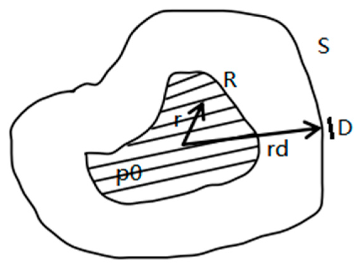
The algorithm proposed in this study is based on coordinate transformation and interpolation techniques. The detailed process and algorithm for this transformation are described as follows:

The Cartesian image $I(x,y)$, with dimensions $\left[N\times N\right]$, assumes that the origin $(0,0)$ is located at the center of the image. For any Cartesian coordinate $(x,y)$, its mapping to the polar coordinate $(r,\theta )$ is defined as:

$$r=\sqrt{{(x-x_c)}^2+{(y-y_c)}^2}, \theta =\arctan 2(y-y_c,x-x_c)$$

(27)

where $(x_c,y_c)$ is the center of the image, typically $x_c={\displaystyle \frac{N}{2}}$ and $y_c={\displaystyle \frac{N}{2}}$. The radial coordinate $r$ represents the distance of a point from the center, while the angular coordinate $\theta$ denotes the angle between the point and the x-axis, usually ranging from $[0,2\pi ]$.

For the target polar coordinate image $I(r,\theta )$, the discrete resolutions of $r$ and $\theta$ are $R$ and $\mathrm{\Theta }$, respectively. The inherent lack of direct one-to-one correspondence between polar grid points $(r,\theta )$ and Cartesian pixels $I(x,y)$ in polar coordinate systems necessitates pixel value estimation through interpolation. The bicubic interpolation method adopted here uses 16 adjacent pixels to maintain superior detail preservation and conversion accuracy.

The bicubic interpolation formula can be expressed as:

$$I(r,\theta )={\displaystyle \sum _{i=-1}^2{\displaystyle \sum _{j=-1}^2\omega (i,\mathrm{\Delta }x)}\cdot \omega (j,\mathrm{\Delta }y)}\cdot I(x_i,y_j)$$

(28)

In the bicubic interpolation formula, $(x_i,y_j)$ represents the coordinates of neighboring pixels in the Cartesian image, which are used to calculate the intensity value at the interpolation point. The offsets of the interpolation point are defined as $\mathrm{\Delta }x$ and $\mathrm{\Delta }y$, the offsets of the interpolation point; $\omega (i,\mathrm{\Delta }x)$ and $\omega (j,\mathrm{\Delta }y)$ are the weight functions that depend on the offsets $\mathrm{\Delta }x$ and $\mathrm{\Delta }y$, respectively.

The weight function $\omega (k,\mathrm{\Delta })$ is defined as [34]:

$$\omega (k,\mathrm{\Delta })=\left\{\begin{array}{c}1.5{\left|\mathrm{\Delta }\right|}^3-2.5{\left|\mathrm{\Delta }\right|}^2+1,\\ -0.5{\left|\mathrm{\Delta }\right|}^3+2.5{\left|\mathrm{\Delta }\right|}^2-4\left|\mathrm{\Delta }\right|+2,\\ 0\end{array}\right.\begin{array}{c}if\left|k\right|\le 1\\ if1<\left|k\right|\le 2\\ if\left|k\right|>2\end{array}$$

(29)

The error of bicubic interpolation converges at a rate of O(d⁴), meaning that, as the sampling spacing d decreases, the interpolation error rapidly approaches zero [34]. Therefore, bicubic interpolation provides a reliable approximation of pixel values during the coordinate transformation process.

The algorithm for converting from polar to Cartesian coordinates involves reversing the mapping process used for Cartesian to polar conversion.

4. Test and Discussion

In this section, we use K-Wave to simulate the generation of blurred pressure distribution images in PAI and test the proposed algorithm to verify its validity [35]. First, we validate the algorithm by calculating a small number of initial pressure distributions, which involves computing the eigenvalues and the eigenvectors corresponding to the minimum eigenvalue. Based on these results, we estimate the blurring kernel. The estimated blurring kernel was then applied to the deblurring process, effectively restoring a clear pressure distribution image. Furthermore, this section explores how to improve the efficiency and accuracy of blurring kernel estimations by selecting an appropriate number of radial column samples from the blurred pressure distribution in the polar coordinate system. To further evaluate the algorithm’s performance, we compared it with the traditional Wiener deconvolution method. The results demonstrated that the proposed deconvolution method outperformed the Wiener deconvolution method in terms of processing accuracy and image quality. Finally, to better reflect real-world scenarios, simulated noise was introduced during the tests to comprehensively assess the robustness and performance of the optimized algorithm under complex conditions.

4.1. Ability to Calculate $h(\varphi )$ Without Noise

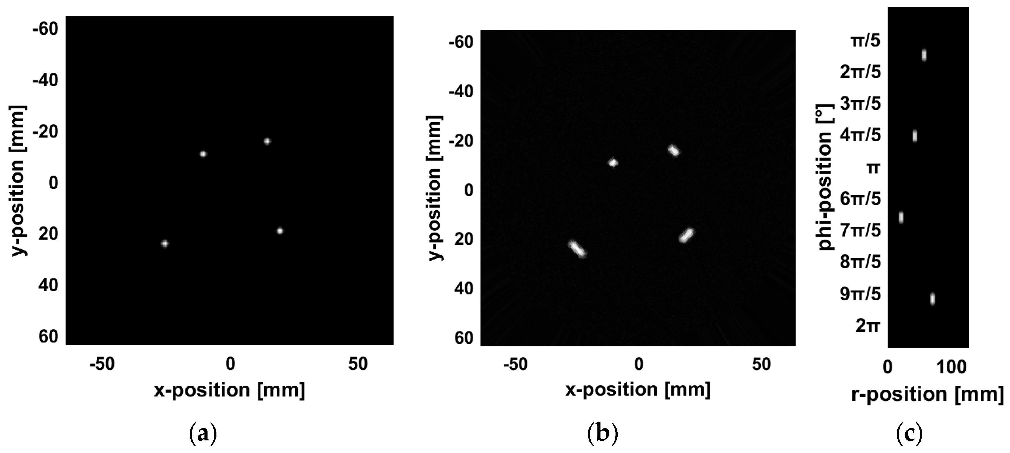
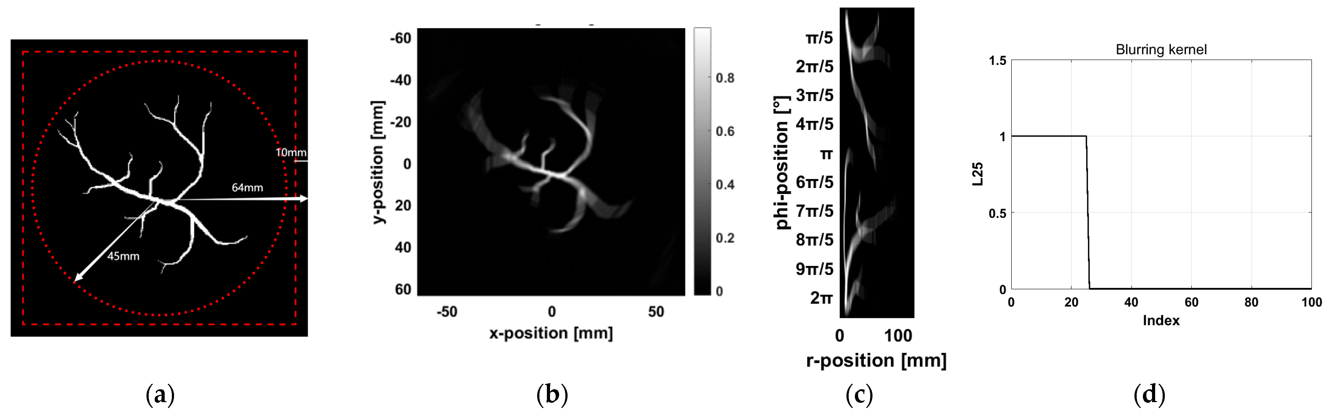
To reduce the computational load, this simulation is conducted in a two-dimensional space. The initial pressure of the vascular model is loaded from an image and scaled accordingly, using a computational grid discretized into 256 × 256 pixels (128 × 128 mm), with a grid spacing of 0.5 mm. To satisfy boundary conditions, a perfectly matched layer (PML) with a thickness of 20 grid cells is applied. The vascular model is positioned at the center of the computational grid. A total of 120 detectors are arranged uniformly along a circular trajectory with a radius of 45 mm to simulate the signal acquisition configuration of a PAI system. Each detector is assumed to be a point detector, with its specific arrangement shown in Figure 4a. In the simulation, the speed of sound is set to 1500 m/s, and the optical absorption coefficient of the vascular model is defined as 1 mm⁻¹. To simplify the computation, the medium is assumed to be acoustically homogeneous, with no sound absorption or scattering. The simulation environment is considered nearly ideal, accounting only for the SIR while ignoring other noise sources. In practical applications, variations in detector size affect the SIR, which in turn influences the PSF of the reconstructed image.

To simulate the circle detector PAI system, we set the angular coverage of the detector to $2\theta ={10}^{°}$, corresponding to a box function with $2\theta ={10}^{°}$. We then convolved the image with the blurring kernel. Figure 4b shows the image after blurring, Figure 4c shows the result after converting the blurred image into polar coordinates, and Figure 4d displays the blurring kernel used for the convolution.

The method we propose for extracting blurring kernels from polar-coordinate pressure distributions involves coordinate transformation using bicubic interpolation. With the O (d⁴) error convergence characteristic of bicubic interpolation, the interpolation error under a grid spacing of d = 0.5 mm remains below 10⁻³ pixel intensity levels. This error is within an acceptable range for the blurring kernel extraction computation.

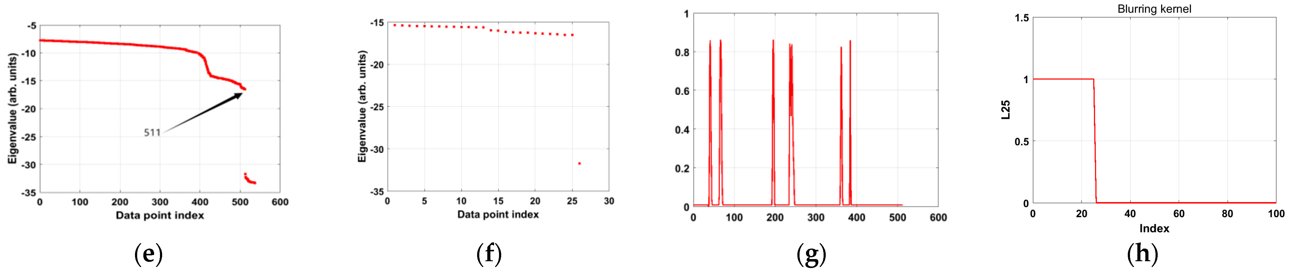
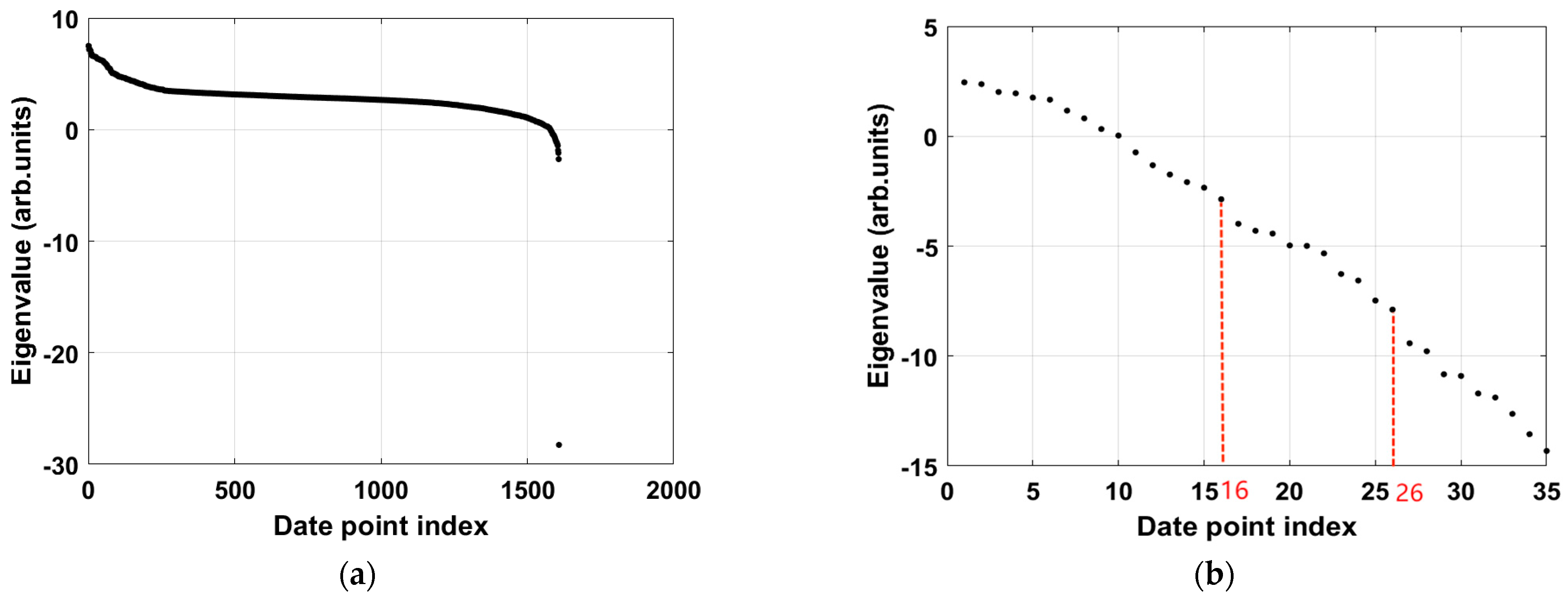
In the tests conducted in this section, we successfully extracted the blurring kernel using the proposed algorithm and reconstructed a clear image. First, we calculated the eigenvalues to determine the length of each column of data in the real discrete initial pressure distribution image. The length of the blurred pressure data in the polar coordinate image used in this study is 536. Therefore, we assumed the length of the initial pressure data to be 536 and compared the sizes of the smallest 536 eigenvectors.

Figure 5a shows the distribution of eigenvalues in logarithmic coordinates. It can be observed that, after the 511th eigenvalue, there is a significant drop, and the eigenvalues after this point are much smaller than the earlier ones. This indicates that the eigenvalues from the 512th to the 536th are close to zero and can be considered zero, totaling 25 zero eigenvalues. This step confirmed that the length of the blurring kernel is 25. Considering the relationship between the blurred pressure distribution, the initial pressure distribution, and the blurring kernel, $M=K+L-1$.

We considered the relationship between the discrete lengths of the blurred pressure distribution, the initial pressure distribution, and the blurring kernel: $M=K+L-1$. We determined the length of the initial pressure distribution to be $K=512$. When only one zero eigenvalue exists, the initial pressure distribution can be accurately determined. Figure 5b shows the relative magnitude of the 25 smallest recalculated eigenvalues, where it is clear that the final eigenvalues are much smaller than the others. The vector corresponding to this eigenvalue represents the estimated initial pressure distribution. Finally, Figure 5c compares the reconstructed radial distribution curve of the initial pressure with the assumed initial pressure distribution curve. The results show that the reconstructed pressure distribution curve closely matches the true initial pressure distribution curve, thereby verifying the accuracy of the algorithm in reconstructing the initial pressure distribution.

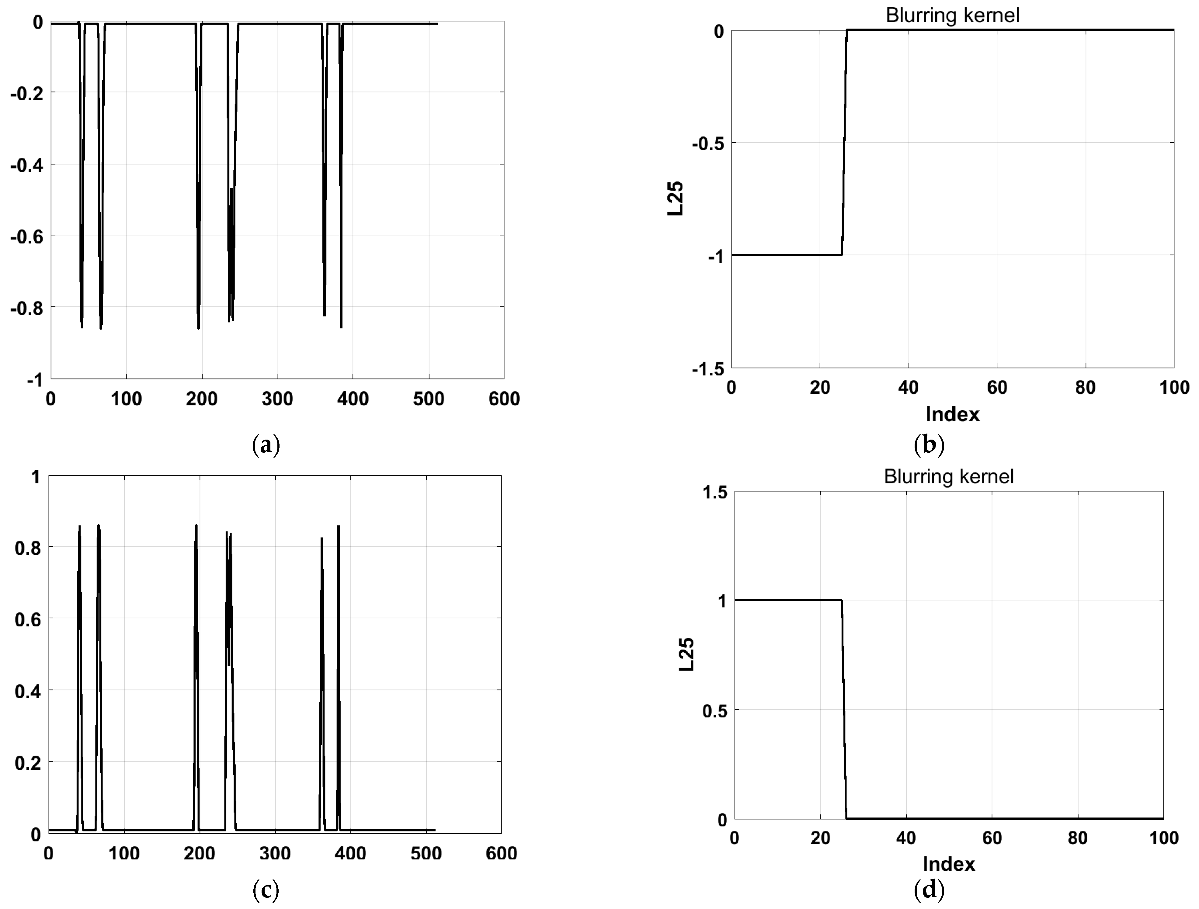
4.2. The Influence of the Number of Bluured Pressure Distributions on the Results

In the algorithm section, we mentioned using two columns of data for the blurring kernel estimations ($j=57,58$). To validate the effectiveness of this approach, we selected two columns of data with abundant and effective information from the polar coordinate image. The selection of these two columns was based on their significant structural features within the image, which provided sufficient information to support the calculation of the blurring kernel while avoiding the inclusion of excessive irrelevant information that could introduce computational interference. This selection method reflects the need for data representativeness. However, in some cases, the initial part of the calculated initial pressure distribution $p_j^0(\varphi )$ exhibited a downward trend that was inconsistent with the actual situation, as shown in Figure 6a,b. To address this issue, we hypothesized that a sign error might have occurred during the calculation.

Therefore, a negative sign was added to $p_j^0(\varphi )$ for correction, and the corrected results are shown in Figure 6c,d. By convolving the corrected $p_j^0(\varphi )$ with the blurring kernel $h_{\theta }(\varphi )$, the final calculation results matched the blurred pressure distribution data exactly, validating the reliability of the method.

To further evaluate the computational efficiency and accuracy of using two columns of data, we tested the effects of using more data columns. Figure 7 illustrates the feature value calculation results for different numbers of data columns. Figure 7a–d shows the relative sizes of the 536 feature values calculated using three columns of data, while Figure 7e–h presents the results for four columns of data. Regardless of whether three or four columns of data were used, the 25 recalculated feature values showed no significant improvement in accuracy compared to the results obtained using two columns of data.

We conducted quantitative analyses using the computation time, peak signal-to-noise ratio (PSNR), and structural similarity index (SSIM). As shown in

Table 1. Computational efficiency and image quality metrics versus varying data column numbers.

Number of Columns	Computation Time (s)	PSNR (dB)	SSIM
2	3.53	32.09	0.9823
3	21.04	33.56	0.9860
4	73.53	34.44	0.9872

, processing with two columns of data required 3.53 s, while using three and four columns increased the computation time to 21.04 s and 73.53 s, respectively. However, the PSNR only improved from 32.09 dB to 33.56 dB and 34.44 dB, and the SSIM increased from 0.9823 to 0.9860 and 0.9872. Although there was a marginal improvement in accuracy, the additional computational cost outweighed the benefits.

Based on the above analysis, it can be concluded that selecting two columns of data with abundant effective information not only ensures sufficient accuracy in the calculation but also significantly improves computational efficiency.

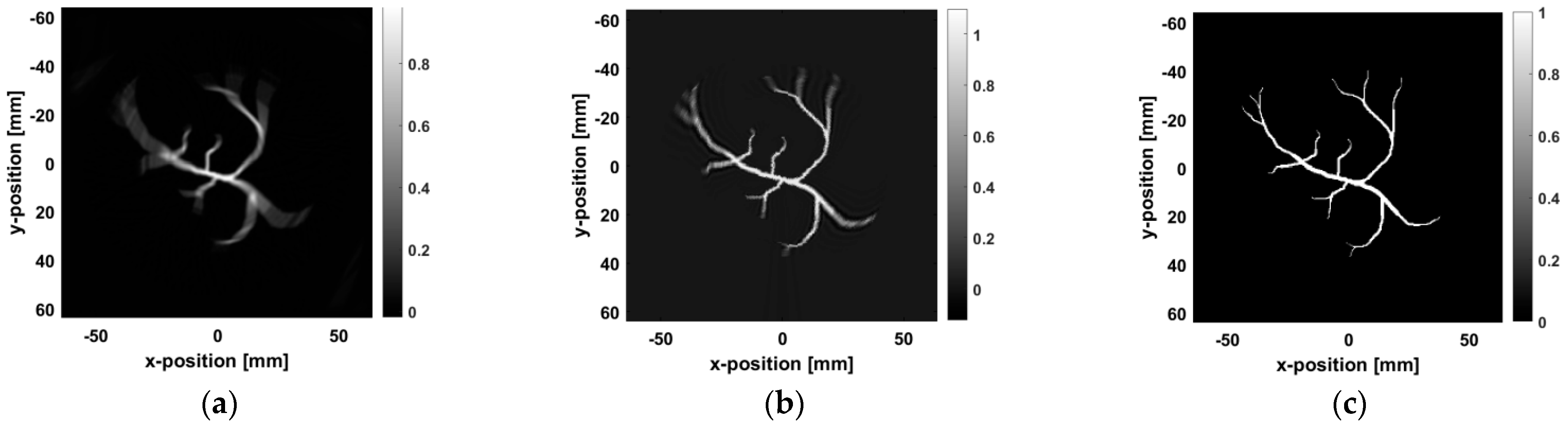
4.3. Comparison with Wiener Deconvolution

The method proposed in this study was compared with Wiener deconvolution, and the results demonstrate that the proposed approach is more effective in reducing blur and enhancing image edge details. Figure 8a shows the blurred image. Although the general shape of the blood vessels is visible, the image suffers from edge blurring and unclear details. Figure 8b shows the results after Wiener deconvolution, where the blur is somewhat reduced. However, due to the limitations of Wiener deconvolution in processing high-frequency image details, especially its tendency to confuse edges and details with noise during the estimation process, the edges and details of the image are excessively smoothed, making it impossible to preserve the original features accurately. As a result, as shown in Figure 8b, the edges of the blood vessels remain unclear. Figure 8c presents the image processed using the proposed method, where significant improvements in edge sharpness, a noticeable reduction in artifacts, and more precise blood vessel details can be observed.

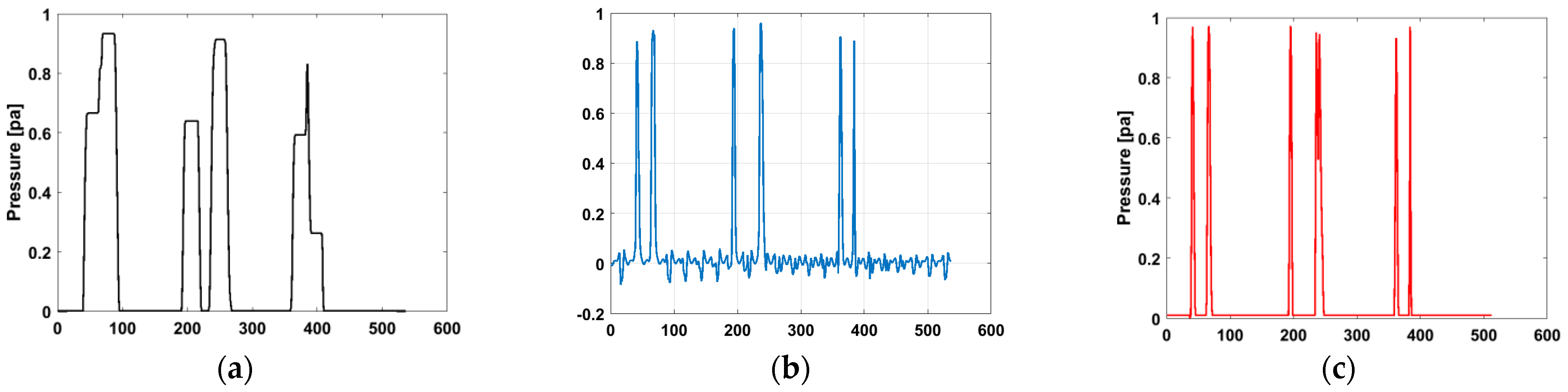
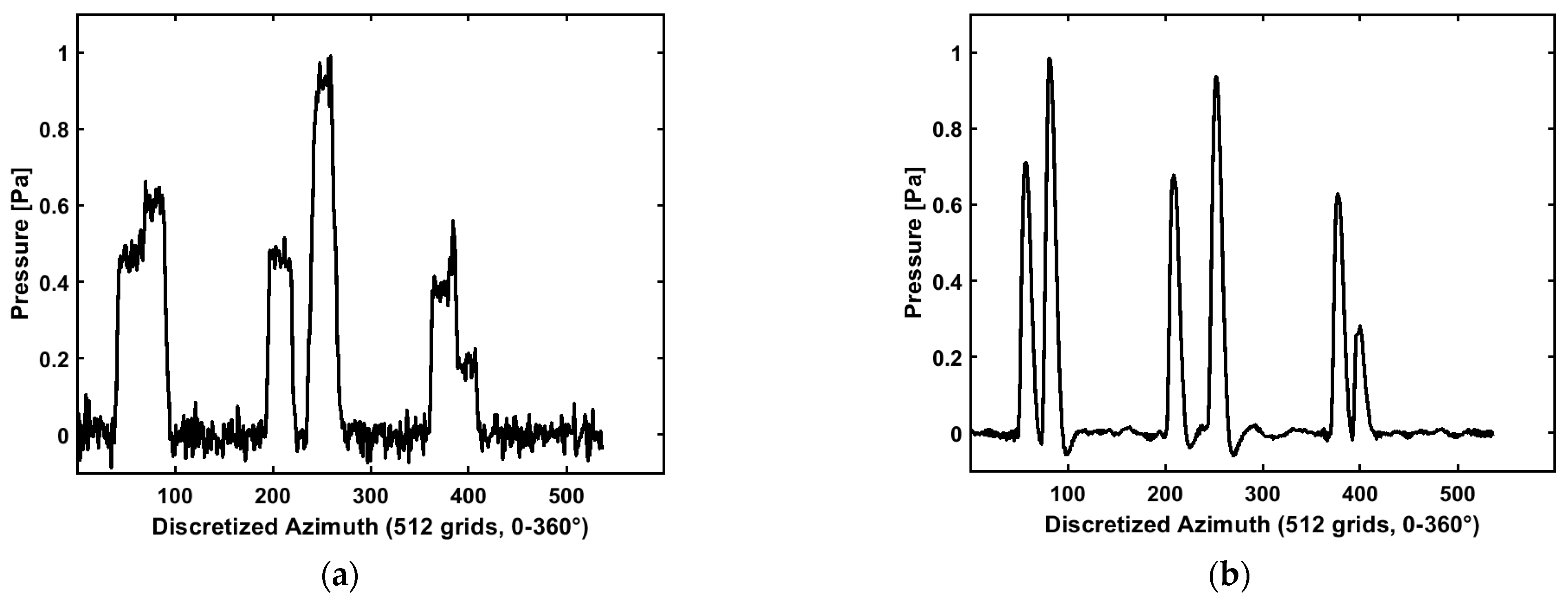
Figure 9 illustrates a comparison of the blurred pressure distribution profile $p_j^{\theta }(\varphi )$, the pressure distribution profile $p_j^0(\varphi )$ calculated using the proposed algorithm, and the one $p_j^W(\varphi )$ calculated using the Wiener deconvolution algorithm $(j=57)$. As shown, the polar pressure distribution profile in Figure 9a appears relatively “smooth”, lacking the delicate and sharp details commonly observed in accurate reconstructions, and it exhibits an overall blurred and smooth appearance. The profile processed by the Wiener deconvolution algorithm (Figure 9b) demonstrates clearer and sharper features but is accompanied by noticeable fluctuations, i.e., noise, which negatively affects the overall quality. In contrast, the profile obtained using the proposed algorithm (Figure 9c) excels in detail recovery, especially in reconstructing edge features and delicate structures, and it aligns more closely with the original assumed initial pressure distribution profile.

Table 2. Quantitative evaluation of image quality for different processing methods (under noise-free conditions).

Image Condition	PSNR (dB)	SSIM
Blurred image	10.41	0.6245
Wiener deconvolution image	23.26	0.7866
Processed image (proposed)	32.09	0.9823

presents the quantitative evaluation results using the PSNR and SSIM metrics to compare the image quality under different processing methods.

The blurred image had a PSNR of 10.41 dB and an SSIM of 0.6245. The Wiener deconvolution method improves the image quality with a PSNR of 23.26 dB and an SSIM of 0.7866, but the proposed method outperforms it, achieving a PSNR of 32.09 dB and an SSIM of 0.9823. This indicates a significant enhancement in image quality, particularly in recovering fine details and edge features, with PSNR improving by 8.83 dB and SSIM increasing by 0.1957 compared to the Wiener deconvolution results. Overall, the proposed method significantly improves the clarity and accuracy of photoacoustic images, particularly in high-resolution imaging tasks. Compared to the Wiener deconvolution algorithm, it demonstrates superior performance in recovering image details and edge features.

4.4. Algorithm Performance Testing in a Noisy Environment

Gaussian noise with an SNR of 40 dB was added to the simulation data, and the improved algorithm’s feasibility and robustness were tested. Columns 57, 58, and 67 of the pressure distribution were chosen as test data due to their rich information and their tail values, which were close to zero, reducing the impact of noise on performance.

In the first step of the optimization algorithm, eigenvalue decomposition was performed on the constructed matrix, as shown in Figure 10a. Apart from the smallest eigenvalue, the remaining eigenvalues exhibit a stable decay trend. To analyze the variations in the tail region, after removing the last abrupt drop in the eigenvalue, the variations between the preceding eigenvalues can be observed more clearly, resulting in a more accurate estimation of the blurring kernel, as shown in Figure 10b. Through the analysis of Figure 10b, it can be observed that the eigenvalues gradually decrease without the noticeable “jump” seen in the noise-free case, which typically indicates the determination of the blurring kernel length. However, some “inflection points” can still be observed, where the difference between certain eigenvalues is more significant than the difference between others. An inflection point appears at the 26th eigenvalue, which suggests that the blurring kernel length may be too short; another inflection point occurs at the 15th eigenvalue, which corresponds to a more reasonable blurring kernel length. Therefore, we determine that L = 20. Although the blur length was set to L = 25 during the simulation, the actual blurring kernel of the noisy image is significantly affected by the noise in the data. During the optimization process, the algorithm interprets part of the original blurred distribution (especially the weaker signal components) as part of the initial pressure distribution rather than an extension of the blurring kernel. In this case, the blurring kernel length calculated according to the optimization algorithm will be shorter.

After determining that L = 20, the algorithm proceeded to the second step, where the eigenvector corresponding to the smallest eigenvalue was used to reconstruct the initial pressure distribution. This eigenvector was decomposed into three groups of pressure sequences, and the LS method was applied to calculate the blurring kernel and deblur the entire image, yielding the processed pressure distribution image.

Figure 11 shows the comparison results of pressure distribution curves before and after denoising processing: (a) the pressure distribution curve with noise exhibits significant blurring kernel effect and noise interference, and (b) after being processed using the optimization method proposed in this article, the pressure distribution curve exhibits more accurate feature extraction.

In the absence of noise and when the blurring kernel is error free, the LS can serve as an effective approach for recovering the acoustic pressure distribution. However, in practical applications, both the observed data and the blurring kernel are typically subject to errors, and the least squares method cannot handle the errors in the blurring kernel effectively, resulting in the inability to completely eliminate the influence of the blurring kernel. This issue relates to the ill-posed nature of inverse problems. To address this, we will further explore the field of inverse problems in the future.

Figure 12 further compares the processing effects under noisy conditions through images: (a) the original pressure distribution image affected by noise and blurring kernels and (b) the reconstruction results after applying the improved algorithms. The test results show that the improved algorithm significantly suppresses the interference of noise and blurring kernels and substantially improves the clarity of the vascular contours.

Table 3. Quantitative comparison of image quality under noisy conditions.

Image Condition	PSNR (dB)	SSIM
Blurred image	8.80	0.2615
Processed image	14.98	0.7113

presents a quantitative evaluation of image quality under noisy conditions. The PSNR of the blurred image under noisy conditions is 8.80 dB, and the SSIM is 0.2615. After applying the proposed blurring kernel extraction method under noisy conditions, the processed image shows improved metrics: the PSNR increases to 14.98 dB while the SSIM rises to 0.7113. Although the PSNR remains relatively low, the substantial improvement in SSIM demonstrates the effectiveness of our method in enhancing the overall image structure and visual coherence. Therefore, the proposed blurring kernel extraction method proves successful in addressing noise-related challenges in deblurring tasks.

4.5. Validation with a Digital Breast Phantom Based on Clinical MRI Data

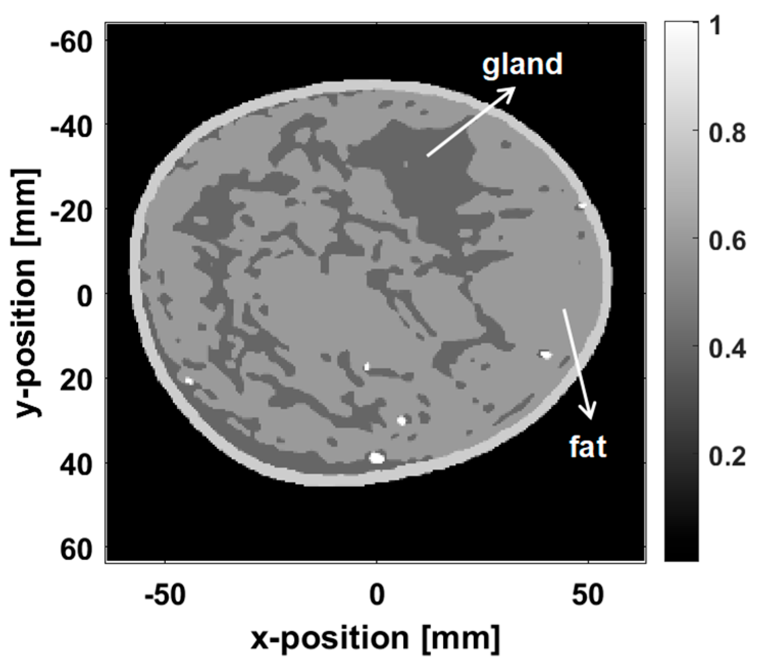
To bridge the gap between idealized simulations and real-world PAI challenges, we further validated our method using an open-source breast phantom derived from clinical MRI data (Washington University School of Medicine) [36]. This breast phantom, constructed based on clinical data, accurately reflects the distribution of breast tissues, including fibroglandular and adipose tissues, providing a more representative testing scenario than that offered by traditional simulations. Figure 13 shows the y–z cross-section of the digital breast phantom at x = 4 × 10⁻² m, realistically simulating the photoacoustic response of breast tissue.

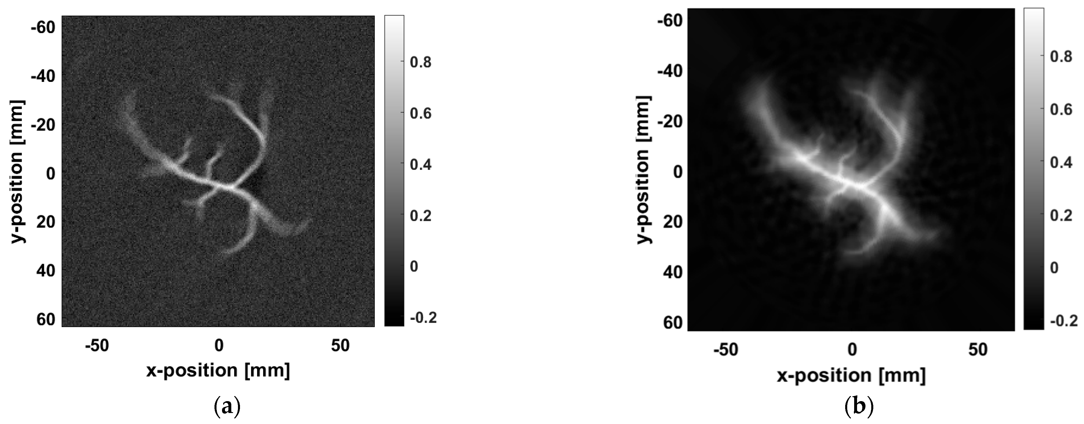
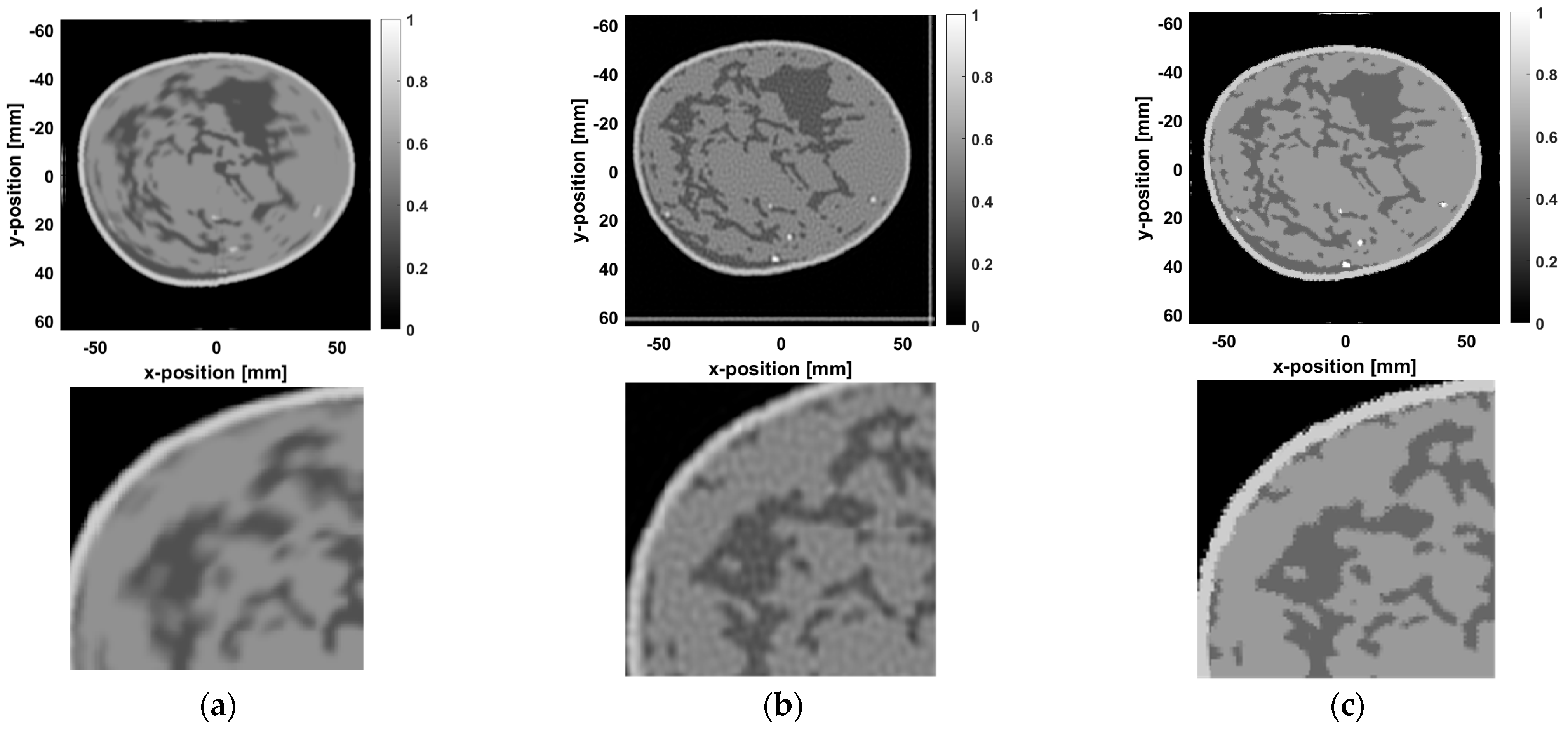
As shown in Figure 14, we present the unprocessed blurred image, the image after Wiener deconvolution, and the image processed using the proposed method, along with their magnified views. In the unprocessed blurred image (Figure 14a), noise and blur effects are quite prominent, and significant detail is lost. The magnified view shows an unnaturally smooth transition between adipose tissue and fibroglandular tissue, which affects the diagnostic quality of the image.

The image after Wiener deconvolution (Figure 14b) shows improvement in noise suppression, but magnification still reveals subtle blurring, especially at the interface between the adipose and fibroglandular tissues. The blur effect remains noticeable, and some regions suffer from detail loss, with no fundamental improvement in image quality.

In contrast, the image processed using the proposed method (Figure 14c) demonstrates significant improvements. The magnified view shows sharper boundaries for the fibroglandular tissue, with more precise restoration of tissue structures. The transition between adipose and fibroglandular tissues is smoother and more natural, with clearer boundaries between different tissue types. Noise and artifacts are effectively suppressed, leading to a substantial improvements in overall image quality.

To further quantify the performance of the proposed method, as shown in

Table 4. Quantitative comparison of objective metrics for breast photoacoustic images under different processing methods.

Processing Method	PSNR (dB)	SSIM
Blurred image	16.81	0.4941
Wiener deconvolution image	22.61	0.5164
Processed image (proposed)	36.77	0.9912

, the unprocessed image exhibits a low PSNR (16.81 dB) and SSIM (0.4941), indicating significant noise and blur, along with poor structural fidelity. After applying Wiener deconvolution, the PSNR and SSIM values improve to 22.61 dB and 0.5164, respectively. Although there is an improvement, some blur remains, particularly in detail recovery. In contrast, the proposed method achieves PSNR and SSIM values of 36.77 dB and 0.9912, respectively, showing a significant improvement in quality, especially in the recovery of fibroglandular tissue details and overall tissue structure.

As seen from the results above, the proposed method achieves a good balance between deblurring and structural fidelity, validating the effectiveness of the algorithm in real breast photoacoustic imaging.

5. Conclusions

This study proposes a PSF estimation method based on coordinate transformation and polynomial standard factor extraction. The algorithm simplifies the complexity of extracting spatially varying PSFs by transforming the image into polar coordinates. It estimates the blurring kernel from the blurred pressure distribution, effectively eliminating the influence of the blurring kernel. Using deconvolution, the influence of the blurring kernel is removed from the photoacoustic image. Test results show that the PSF extracted using this method can effectively be applied to the deblurring of photoacoustic images affected by circular integral detectors, significantly reducing “spin blurring” and restoring image edges and details. This algorithm supports the selection of two columns of pressure data to save computation time when solving blurring kernel problems. Its high reconstruction accuracy, low computational complexity, and strong robustness make it suitable for photoacoustic imaging systems constrained by the size of ring detectors and noise. Furthermore, the method has demonstrated promising results in breast photoacoustic imaging, where it helps to recover fine details and improve structural fidelity in complex tissue structures. Future work will test it on real photoacoustic data and improve its robustness to noise through optimized regularization techniques for deconvolution.