Dynamic Modeling of a Compressed Natural Gas Refueling Station and Multi-Objective Optimization via Gray Relational Analysis Method

Abstract

Compressed natural gas (CNG) refueling stations operate under highly dynamic thermodynamic conditions, requiring accurate modeling and optimization to ensure efficient performance. In this study, a dynamic simulation model of a CNG station was developed using MATLAB-SIMULINK, including detailed subsystems for multi-stage compression, cascade storage, and vehicle tank filling. Real gas effects were incorporated to improve prediction accuracy of the pressure, temperature, and mass flow rate variations during fast filling. The model was validated against experimental data, showing good agreement in both pressure rise and flow rate evolution. A two-stage multi-objective optimization approach was applied using Taguchi experimental design and gray relational analysis (GRA). In the first stage, storage pressures were optimized to maximize the number of vehicles filled and gas mass delivered, while minimizing compressor-specific work. The second stage focused on optimizing the volume distribution among the low, medium, and high-pressure tanks. The combined optimization led to a 12.33% reduction in compressor-specific energy consumption with minimal change in refueling throughput. These results highlight the critical influence of pressure levels and volume ratios in cascade storage systems on station performance. The presented methodology provides a systematic framework for the analysis and optimization of transient operating conditions in CNG infrastructure.

1. Introduction

In the global transition toward cleaner energy systems, compressed natural gas (CNG) continues to serve as a viable alternative fuel for the transportation sector due to its relatively low emissions, mature infrastructure, and economic feasibility [1]. Compared to conventional fuels, CNG exhibits superior combustion characteristics and environmental benefits, particularly in urban mobility applications [2,3,4]. Its usage not only reduces greenhouse gas emissions but also provides a reliable transitional pathway within existing engine technologies [5].

Recent comparative studies have evaluated CNG, battery electric vehicle (BEV), and fuel cell electric vehicle (FCEV) technologies in public transport, emphasizing that CNG remains a competitive and transitional option in terms of both environmental and economic performance [6]. While CNG remains a viable low-emission alternative in many urban freight applications, recent cost–benefit analyses suggest that electric light commercial vehicles (LCVs) may offer lower total cost of ownership under certain conditions. For example, Bhutani et al. [7] found that EVs had a cost advantage of 2% over CNG vehicles in urban distribution scenarios, although infrastructure and policy support remain critical factors in the adoption process.

In addition to performance considerations, recent research has also explored the safety and risk aspects of CNG infrastructure by applying integrated decision-making methods. For example, Ali et al. [8] analyzed the CNG sector in Pakistan using fuzzy AHP and TOPSIS, identifying system design limitations, human error, and economic instability as key issues, especially in developing countries.

Meanwhile, dynamic modeling has become a useful tool for capturing how gas storage and distribution systems respond under variable conditions. Di Nardo et al. [9,10] demonstrated that incorporating time-varying parameters into simulations improves the accuracy of system behavior predictions. In a similar context, Xu et al. [11] used scenario-driven risk assessments to show how dynamic models can support better safety planning in integrated energy systems.

Hybrid systems that combine CNG and electricity are drawing increasing interest, especially in the broader area of multi-energy systems. Seyfi et al. [12] proposed an energy management method that uses deep learning to control a virtual energy hub, which connects vehicles that run on both CNG and electricity with a gas compression station. Their results showed that CNG can help improve system flexibility when used together with electric and thermal energy sources.

At the same time, comparisons between different refueling technologies show a growing focus on hydrogen systems. For example, Chu et al. [13] described a hydrogen station powered by solar energy, which includes an electrolyzer, a compressor, and a storage setup. They also used life cycle and full-chain efficiency analyses to study its environmental and economic impact. These modeling efforts reflect the growing demand for cleaner and more efficient fuel systems.

Simulation tools such as MATLAB and Simulink are widely used in engine and control system development. For instance, Munahar et al. [14] used this platform to evaluate passenger comfort by measuring vibration levels in vehicles that use CNG.

Despite these advantages, the operation of CNG refueling stations introduces several engineering challenges. These include high-pressure storage requirements, energy-intensive compression cycles, transient thermal effects during fast filling, and the need for efficient system control [15,16,17,18]. One of the primary difficulties lies in managing the dynamic behavior of thermodynamic parameters, such as pressure, temperature, and gas density, which vary significantly during the refueling process [19,20,21,22]. Rapid temperature rise due to gas compression can lead to lower fill efficiency, reduced safety margins, and increased energy consumption [23,24,25,26]. Experimental and numerical studies have shown that initial gas conditions, pressure staging, and heat transfer mechanisms play critical roles in determining system performance during fast filling operations [27,28,29,30,31].

In CNG infrastructure, the proper design and control of compressor systems are also crucial. Compressor cycling, control algorithms, and reservoir pressure staging significantly affect station efficiency and operational cost [32,33,34]. Additionally, component-level reliability issues, such as valve material degradation or improper mounting structures, can impact safety and maintenance performance [35,36,37].

Although several studies have addressed individual aspects of CNG station operation, such as fuel transmission [38], energy cost [39,40], and thermodynamic losses [41,42], a comprehensive approach that simultaneously considers multiple engineering objectives, such as pressure level, storage volume allocation, and thermal behavior, remains underexplored [43,44,45].

Another important factor influencing the performance of CNG refueling systems is the optimization of pressure levels and volume distributions within cascade storage configurations. Farzaneh-Gord and Deymi-Dashtebayaz [46] investigated the effects of different pressure stages on station efficiency using an ideal gas model and demonstrated that determining optimal pressure levels can enhance compressor energy usage and refueling time. Similarly, Farzaneh-Gord et al. [47] presented a comprehensive analysis on optimizing the volume ratios of storage tanks in multi-line systems to improve overall station performance. However, most of these studies were conducted under steady-state or quasi-steady assumptions, with limited attention to the dynamic behavior of the system.

In recent years, multi-objective optimization techniques have gained attention as a means to holistically improve energy systems. In particular, the combination of Taguchi experimental design with gray relational analysis (GRA) has proven effective in a wide range of thermal and mechanical applications, such as refrigeration systems [48], battery thermal management [49], absorption cooling [50] and organic Rankine cycles [51]. This approach allows for simultaneous consideration of several conflicting performance metrics, making it highly suitable for systems like CNG refueling stations, where trade-offs between pressure utilization, energy efficiency, and temperature control must be carefully balanced.

In this study, the well-established Taguchi–GRA framework was adapted to optimize a dynamically modeled CNG refueling station. The model evaluates system behavior over a 24 h operating cycle and targets simultaneous optimization of reservoir pressure levels and volume distribution to minimize compressor cycling and ensure sufficient fill pressure for vehicle tanks. All thermodynamic properties of natural gas, including pressure-dependent density and enthalpy, were calculated based on real gas properties to ensure accurate simulation of compression and filling dynamics. This ensures that the simulation reflects the actual behavior of natural gas during compression and filling.

By combining dynamic simulation with multi-objective optimization, this work contributes a novel framework for improving the technical performance, energy efficiency, and operational stability of CNG refueling systems. In doing so, it addresses critical gaps in the current literature and offers insights for future infrastructure development.

2. Materials and Methods

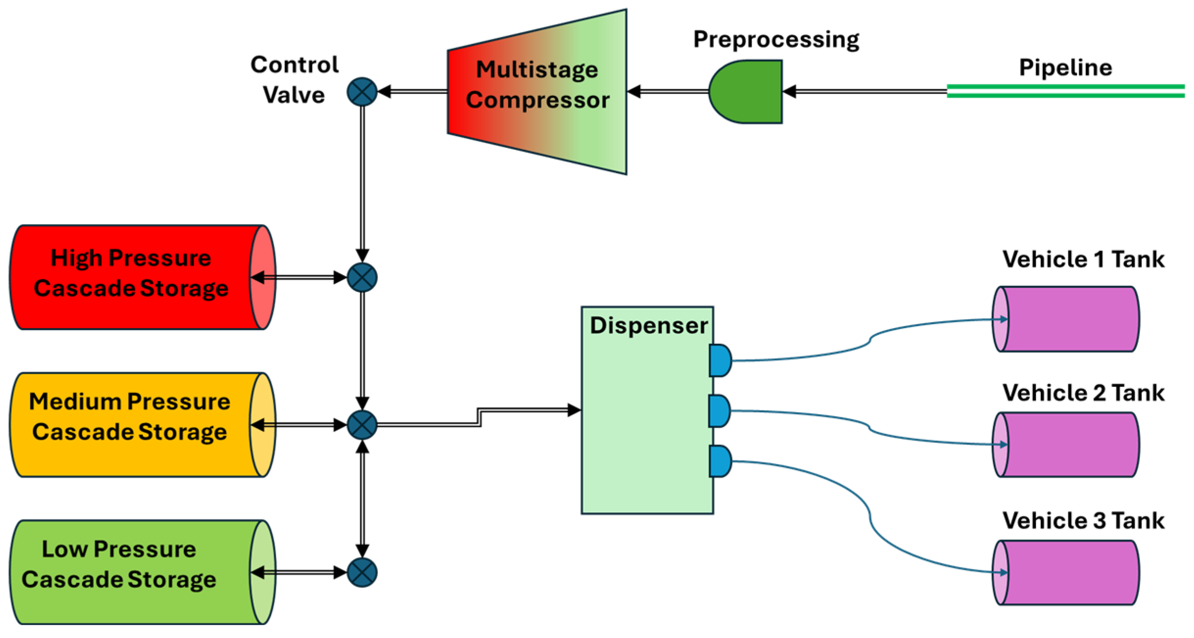
The CNG refueling station model used in this study is shown in Figure 1. It was developed using MATLAB ^® (R2024a)-SIMULINK software. The model simulates the entire refueling process, including gas intake from the natural gas pipeline, compression in the compressor, storage in tanks, and dispensing to vehicles. Additionally, it incorporates a logical control system that manages these operations efficiently.

The pipeline subsystem includes the solver configuration, where essential solver parameters are defined before starting the simulation. It also incorporates a gas properties block, which defines the characteristics of the natural gas, and a reservoir block that sets the initial conditions for gas entering the system. These components are sourced from the gas library and modeled within this subsystem.

In this study, the gas is modeled as a real gas, specifically pure methane. However, perfect gas properties are also used for validation against experimental data, with the ideal gas law applying to perfect gases.

Table 1. Physical properties for methane as an ideal gas.

Physical Properties for Methane as an Ideal Gas
Specific gas constant	0.51827 kJ/(K kg)
Compressibility factor	0.99814
Reference temperature for gas properties	293.15 K
Specific enthalpy at reference temperature	898.82 kJ/kg
Specific heat at constant pressure	2.2206 kJ/(K kg)
Dynamic viscosity	11.037 μPa·s
Thermal conductivity	33.448 mW/(K m)

presents the gas properties of the connected gas network under the assumption of ideal gas behavior. These values correspond to methane at a temperature of 293.15 K and a pressure of 1.01325 bar [52].

For real gas modeling, all properties vary as functions of temperature and pressure, represented as two-dimensional arrays. The selected temperature range for thermodynamic properties extends from 153.15 K to 543.15 K, while the pressure range covers 0.1 to 300 bars. These property arrays are sourced from the open-source CoolProp database [52].

In order to implement real-gas behavior dynamically, a MATLAB Function block was developed to call the PropsSI function from the CoolProp library at each simulation step. This function enables the retrieval of real-time thermophysical properties such as density, specific heat, and enthalpy based on instantaneous temperature and pressure conditions, ensuring consistency with Helmholtz-based equations of state. Compared to fixed tabular data or simplified ideal gas assumptions, this method allows for more accurate and continuous representation of gas behavior during transient processes such as fast-filling. CoolProp’s interpolation algorithms have been validated against NIST reference data and are widely adopted in thermodynamic modeling.

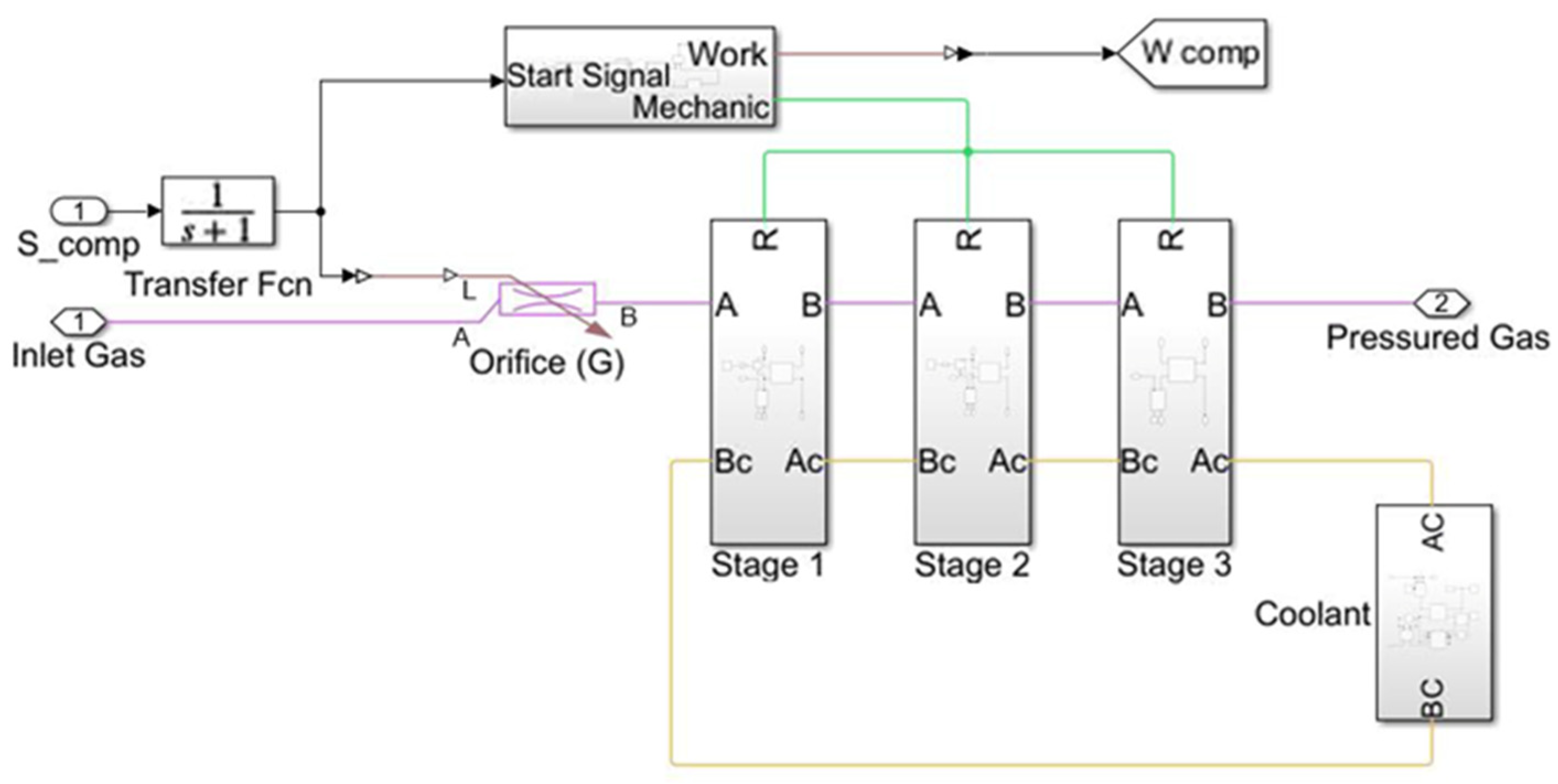
A multi-stage compressor subsystem is shown in Figure 2. This subsystem shows the operating principle of a compressor system. The signal from the control unit passes through a transfer function and is subjected to a process that determines the dynamic response of the system. The gas then flows through an orifice, where the flow is regulated and directed to a three-stage compression system. The orifices used here and throughout the system are modeled with a gas library.

At each stage, the gas is pressurized and passed to the next stage. This process ensures an efficient compression process by gradually increasing the pressure. The cooling system is also in operation and contributes to the healthy operation of the system by dissipating the heat generated during compression.

The mechanical operation is initiated by a start signal, which activates the compression process. The system incorporates mechanical rotational reference, ideal angular velocity source, and ideal torque sensor from the mechanical library, ensuring accurate modeling of mechanical dynamics. As a result, the compressor generates mechanical work, ultimately delivering pressurized gas as the final output.

The design parameters used in the development of the compressor system are detailed in

Table 2. CNG compressor parameters.

Positive-Displacement Compressor
Stage 1 Displacement volume	1856 cm3/rev
Stage 2 Displacement volume	862 cm3/rev
Stage 3 Displacement volume	400 cm3/rev
Polytropic exponent	1.3
Nominal volumetric efficiency	0.9
Nominal pressure ratio	10
Mechanical efficiency	0.95
Maximum shaft speed	1000 rpm

, providing insight into the system’s performance characteristics and operational capabilities. These design parameters were selected based on typical specifications of industrial reciprocating compressors commonly used in CNG refueling stations. Although exact values may vary across manufacturers, the chosen values fall within the range observed in publicly available technical documents and are representative of commercial systems operating under similar pressure ratios and flow conditions [53,54].

In particular, the polytropic exponent was set to n = 1.3, which characterizes a partially cooled gas compression process with intercooling between stages. This value is thermodynamically realistic, lying between isothermal (n = 1) and adiabatic (n ≈ 1.4) conditions. It has also been validated in experimental studies involving real-gas compression under non-ideal conditions [53].

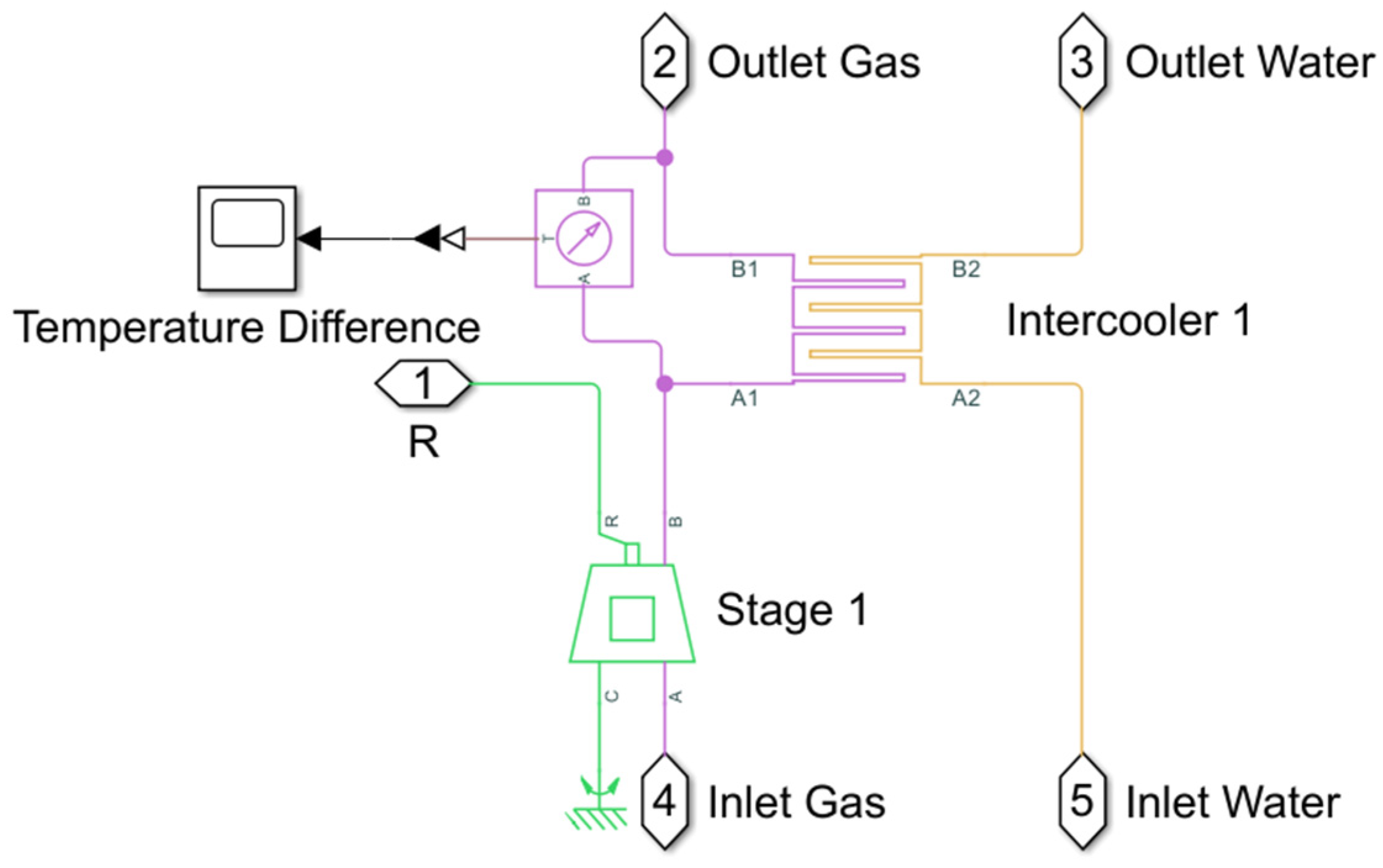
The Stage 1 subsystem, as illustrated in Figure 3, represents the first phase of a multi-stage compression system, with subsequent stages modeled in a similar manner. To regulate the temperature of the compressed gas, an intercooler has been implemented, modeled using the heat exchanger library.

The process begins when the inlet gas enters the first stage of compression. At this stage, the gas is compressed, leading to an increase in both pressure and temperature. Before progressing to the next stage, the compressed gas is directed to the intercooler, where its temperature is reduced to improve efficiency.

The intercooler operates using inlet water, which absorbs heat from the compressed gas, ensuring an effective cooling process. As a result, outlet water carries the heat away from the system, while the cooled gas is delivered as outlet gas, ready for the next stage of compression. Additionally, a temperature difference measurement unit is included in the model to monitor and evaluate the effectiveness of the cooling process by comparing the inlet and outlet temperatures.

This stage plays a critical role in improving the overall efficiency of the system. By reducing the gas temperature between compression phases, the energy required for subsequent compression stages is minimized, while thermal stress on system components is significantly reduced. As a result, the performance and operational lifespan of the compressor system are optimized.

The coolant subsystem is modeled to demonstrate a heat exchange mechanism that includes a cooling system. Heat transfer is achieved using water and air flow, ensuring the regulation of the coolant temperature.

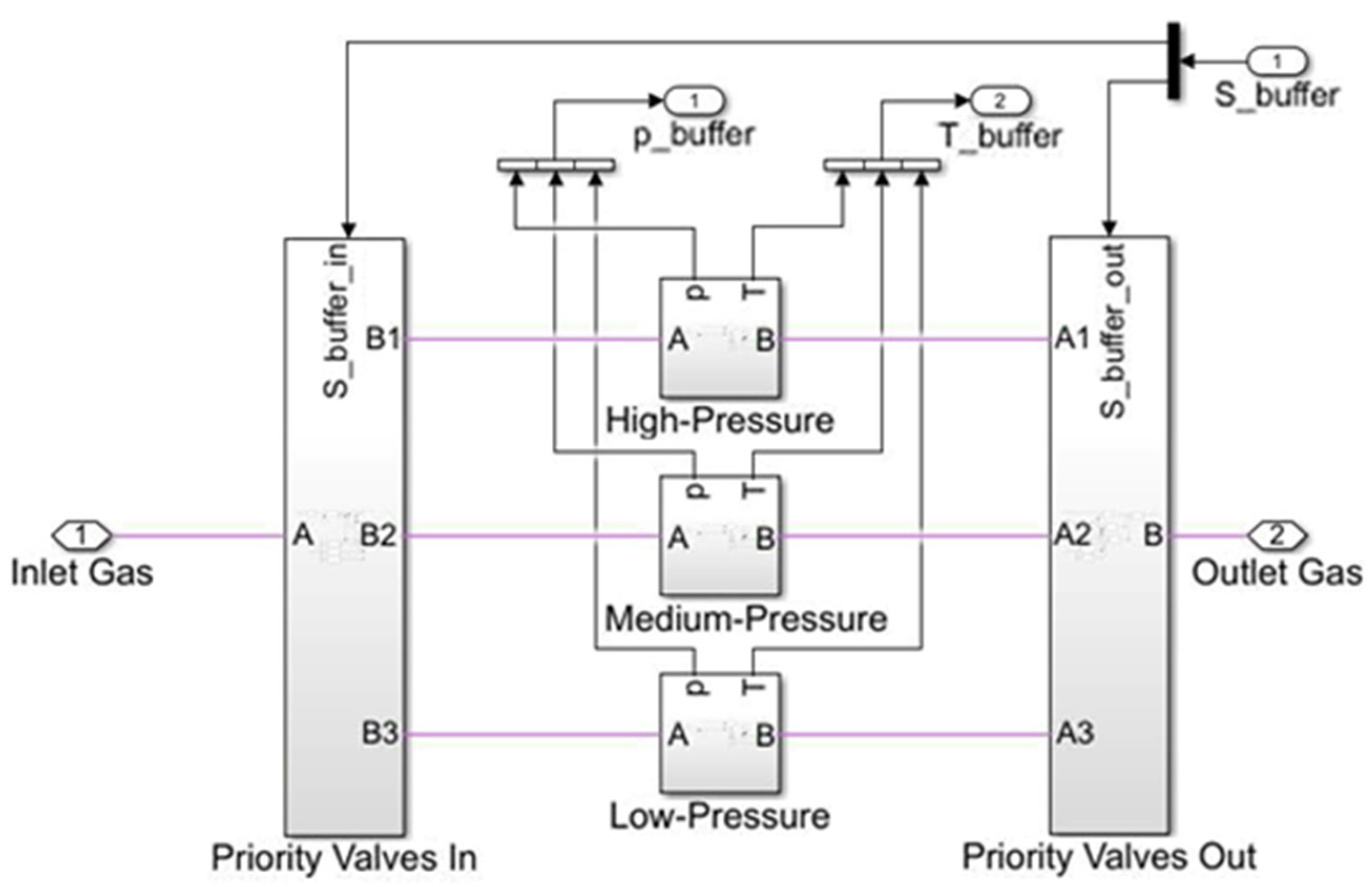
The cascade storage system is divided into three reservoirs, classified as low-pressure, medium-pressure, and high-pressure reservoirs. Each of these reservoirs consists of several large tanks. Figure 4 presents a schematic diagram of the cascade storage system.

On the left side, the “Priority Valves In” subsystem is where the inlet gas enters the system. As the gas passes through this section, it is directed into three different storage levels based on pressure: high-pressure, medium-pressure, and low-pressure. These sections store gas at different levels and regulate the supply according to demand. When the pressure in the high-pressure reservoir reaches the pre-set minimum level, the orifices in the “Priority Valves In” subsystem sequentially fill the low-pressure, medium-pressure, and high-pressure reservoirs. During the filling of the storage tanks, vehicle refueling through dispensers does not occur.

The heat transfer mechanism between the storage tanks and the environment is modeled in the subsystems, and temperature and pressure monitoring is conducted. Thermal mass, conductive heat transfer, and convective heat transfer are modeled using the thermal elements library. Temperature control is modeled using a temperature sensor block, which allows for the analysis of the temperature difference between two desired points without removing heat from the system. The values used in heat transfer and material properties are provided in

Table 3. Parameters for heat transfer at storage and vehicle tanks [55].

Storage and Environment Properties
Tank construction material (Type I)	34CrMo4
Single storage tank capacity	150 L
Vehicle tank capacity	70 L
Empty storage tank weight	125 kg
Empty vehicle tank weight	75 kg
Storage tank outer diameter	370 mm
Storage tank inner diameter	350 mm
Storage tank height	1.8 m
Vehicle tank height	0.9 m
Tank specific heat capacity	561 J/kgK
Tank thermal conductivity	50 W/mK
Internal heat transfer coefficient	300 W/m2K
External heat transfer coefficient	10 W/m2K
Total number of storage tanks	48
Ambient temperature	20 °C

.

On the right side, the “Priority Valves Out” subsystem manages the release of gas from the system. During fast refueling, the vehicle tank is initially connected to the low-pressure reservoir. As the pressure in the reservoir drops and the pressure in the vehicle’s cylinder increases, the gas flow rate decreases. When the flow rate reaches a predefined threshold, the system switches to the medium-pressure reservoir and finally to the high-pressure reservoir to complete the refueling process.

Compared to storing all gas in a single-pressure buffer tank, the cascade system is expected to provide more complete refueling while optimizing the efficiency of both the compressor and the storage tanks. To ensure that vehicle tanks are adequately filled, the high-pressure reservoir must always be maintained at a slightly higher pressure than the target pressure of the vehicle tank.

Proper determination of compressor capacity and cascade storage volume is essential to allow the CNG station to manage vehicle frequency efficiently. Additionally, setting the correct maximum and minimum pressure values for the low, medium, and high-pressure tanks and allocating volumes appropriately ensures the effective operation of the station.

In the dispenser subsystem, the inlet gas serves as the starting point of the system and is directed through a control mechanism. The control unit regulates the inlet valve using a transfer function, which determines the dynamic response of the gas flow, smoothing sudden changes and ensuring a steady flow. The valve is a fundamental component that regulates both the direction and quantity of flow. When opened, gas moves toward the hose, which provides a flexible conduit for directing the flow. The check valve ensures that the gas moves only in the designated direction, preventing backflow and enhancing system safety. Finally, the outlet gas point is where the gas is delivered to vehicles under appropriate pressure and flow conditions. This system is designed to facilitate the controlled and safe distribution of gas. The check valve, hose connection, and control valve are modeled using elements from the gas library.

The three-vehicle subsystem models the vehicle tank filling process and its thermodynamic interactions. During gas transfer, parameters such as mass flow, pressure, and temperature are monitored by sensors to ensure efficient and controlled filling. The inlet point, labeled as dispensed gas, represents the gas line responsible for filling the vehicle tank, where a mass flow rate sensor measures the transfer speed. The pressure sensor monitors the tank’s current pressure, providing real-time data to the control unit, while the temperature sensor detects the gas temperature inside the tank. The vehicle tank is modeled using internal convection and heat conduction mechanisms, where internal convection accounts for heat transfer within the tank, and heat exchange with the surroundings is represented through internal conduction and external convection. The thermal properties of the tank wall are incorporated via the wall mass component, considering conductivity and heat capacity in the heat transfer process. Heat dissipation to the environment is modeled using the conduction tank and external convection components, while the environment temperature component simulates the ambient temperature effects on overall heat transfer. The values and material properties used in the heat transfer calculations are provided in Table 3.

The experimental dataset used for validation in this study was originally presented by George [56], based on a fast-fill CNG operation with cascade storage. This dataset has also been widely used in previous research for benchmarking and validation purposes, notably by Saadat-Targhi et al. [27] and Farzaneh-Gord et al. [47]. In these studies, the model predictions showed high consistency with the experimental results, reinforcing the reliability of the dataset.

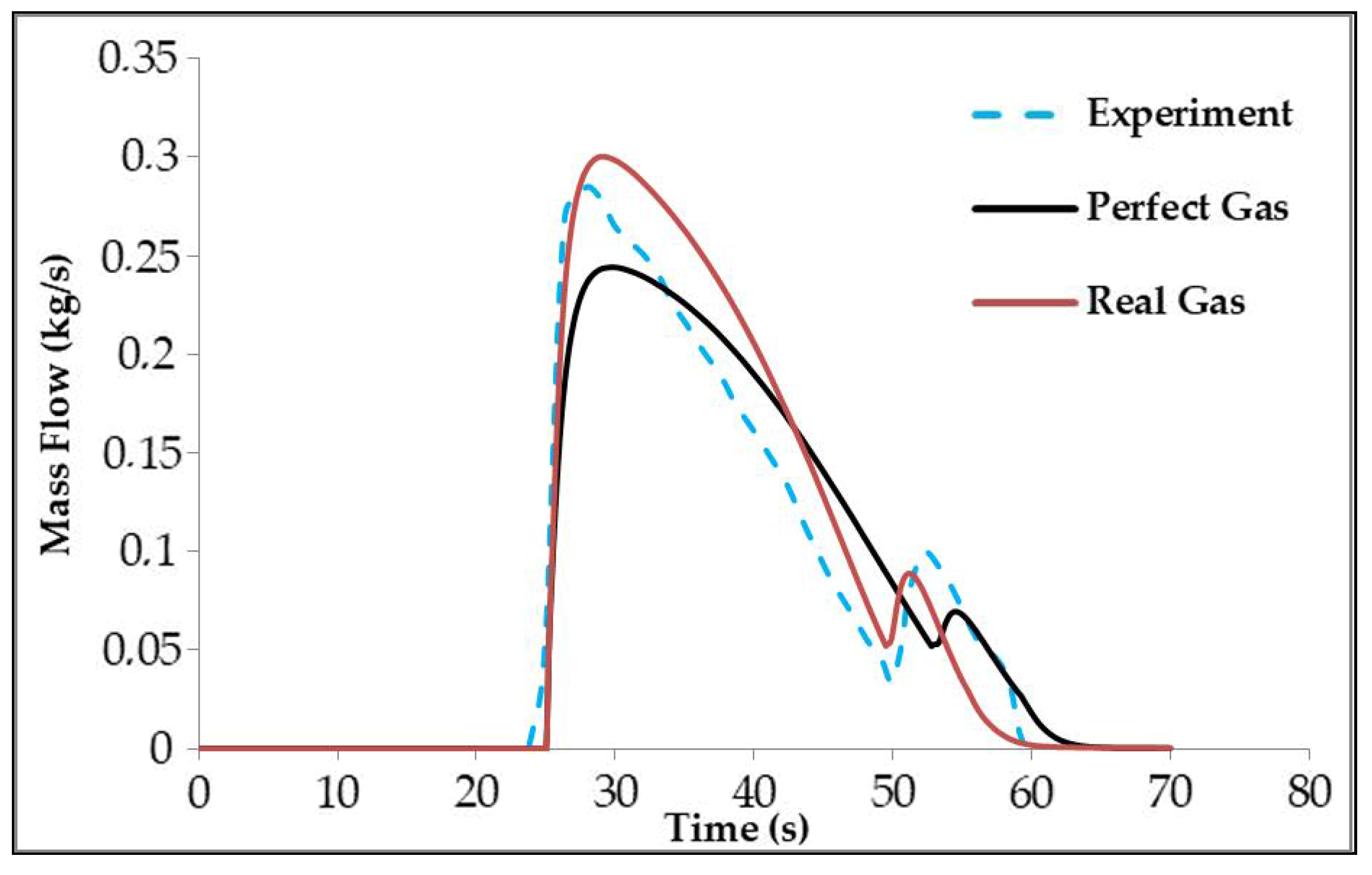
Figure 5 illustrates the variation of mass flow rate over time, comparing the simulation results with the experimental data. The experimental conditions are consistent with those reported in [27,47], where the initial pressure of the NGV cylinder is 72 bar and the volume is 52 L. The mass flow rate varies between 0.29 kg/s and 0.04 kg/s, managed through a cascade storage system. The fast-filling process starts at 24 s and ends at 60 s. The experimental data are shown as a blue dashed line, while the perfect gas and real gas simulation results are represented by black and red lines, respectively.

These results indicate that the real gas model provides a closer alignment with the experimental measurements, especially at the peak flow rate and during the decline phase. The perfect gas model underestimates the maximum flow rate and shows noticeable discrepancies in the decreasing region. These findings confirm that considering real gas behavior improves the accuracy of mass flow predictions during high-pressure filling.

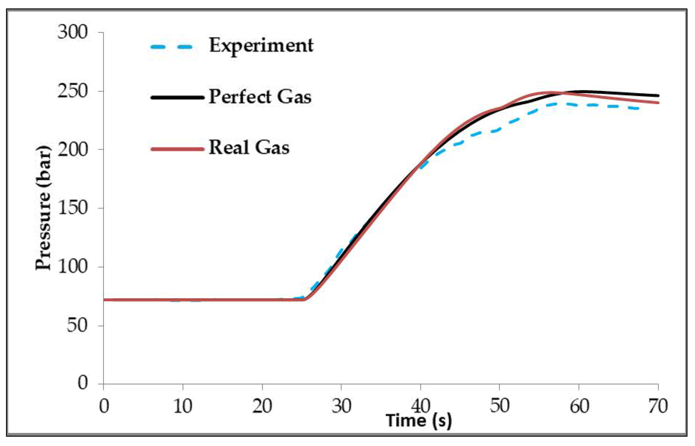
Figure 6 shows the pressure variation in the NGV cylinder over time. Initially, the pressure remains low and then increases rapidly after approximately 24 s. Both gas models (perfect and real) showed a high degree of agreement with the experimental results, particularly during the pressure rise phase. However, the final pressure predicted by both simulations was slightly higher than the experimental values. This is due to the target pressure being set at 250 bar in the simulation, compared to 240 bar in the experimental setup. The real gas model again yielded results closer to the experimental curve, confirming its higher accuracy under dynamic filling conditions. This target pressure difference also accounted for the small deviation observed during the flow decline stage, as the simulation continued for a longer duration to reach 250 bar, leading to slightly higher mass flow values near the end of the process.

The experimental flow rate deviation was approximately ±0.015 kg/s, as also reported by Farzaneh-Gord et al. [47] and Saadat-Targhi et al. [27]. Similarly, the pressure deviation between the simulation and experiment was approximately 10 bar (4.2%), consistent with the target pressure difference observed in George [54]. The total filling time deviation between the simulation and experiment was around 2 s, corresponding to about 5.5% of the total duration.

The Taguchi method, a statistical approach, is a systematic and efficient technique for optimizing design variables. It utilizes fractional designs derived from orthogonal arrays to explore the entire experimental domain with a minimal number of experiments, ensuring efficiency while maintaining accuracy. This method facilitates the identification of optimal conditions, and the conclusions drawn from the Taguchi method are applicable across the entire experimental region.

In this study, the Taguchi method was employed to analyze the pressure and volume arrangements of low-, medium-, and high-pressure storage tanks for the efficient operation of the station. Within the Taguchi design, three control factors were selected to determine the storage tank pressures: high storage tank pressure (P_high), medium storage tank pressure (P_medium), and low storage tank pressure (P_low). Each factor was analyzed at four distinct levels, as detailed in

Table 4. Control factors and levels used in the pressure analysis.

Parameters	Phigh [Bar]	Pmedium [Bar]	Plow [Bar]
Level 1	250	205	130
Level 2	240	185	110
Level 3	230	165	90
Level 4	220	145	70

. These pressure values were evaluated using a four-level design to independently observe their impact at different cascade stages, thereby justifying the selection of an L16 orthogonal array. In the subsequent volume optimization stage, the control factors V_low/V_total and V_medium/V_high were limited to three levels due to the fixed total tank count (48 cylinders) and the physical feasibility of the storage configuration, which led to the use of an L9 orthogonal array. Although no separate sensitivity analysis was performed, the level ranges were carefully selected based on thermodynamic principles, engineering judgment, and previous simulation experience.

The ratio of the pressure storage tank volume (V_low, V_medium, V_high) to the total volume V_total was established for optimal volume distribution in Equations (1)–(3). The remaining volume, after selecting V_low, is expressed as the ratio of the medium-pressure storage tank volume V_medium to the high-pressure storage tank volume V_high in Equation (4) [47]. The volume optimization can be further refined by introducing four dimensionless parameters, defined as follows:

$${\overline{\mathrm{v}}}_{\mathrm{low}}={\displaystyle \frac{{\mathrm{V}}_{\mathrm{low}}}{{\mathrm{V}}_{\mathrm{low}}+{\mathrm{V}}_{\mathrm{medium}}+{\mathrm{V}}_{\mathrm{high}}}}={\displaystyle \frac{{\mathrm{V}}_{\mathrm{low}}}{{\mathrm{V}}_{\mathrm{total}}}}$$

(1)

$${\overline{\mathrm{v}}}_{\mathrm{medium}}={\displaystyle \frac{{\mathrm{V}}_{\mathrm{medium}}}{{\mathrm{V}}_{\mathrm{low}}+{\mathrm{V}}_{\mathrm{medium}}+{\mathrm{V}}_{\mathrm{high}}}}={\displaystyle \frac{{\mathrm{V}}_{\mathrm{medium}}}{{\mathrm{V}}_{\mathrm{total}}}}$$

(2)

$${\overline{\mathrm{v}}}_{\mathrm{high}}={\displaystyle \frac{{\mathrm{V}}_{\mathrm{high}}}{{\mathrm{V}}_{\mathrm{low}}+{\mathrm{V}}_{\mathrm{medium}}+{\mathrm{V}}_{\mathrm{high}}}}={\displaystyle \frac{{\mathrm{V}}_{\mathrm{high}}}{{\mathrm{V}}_{\mathrm{total}}}}$$

(3)

$${\overline{\mathrm{v}}}_{\mathrm{m}/\mathrm{h}}={\displaystyle \frac{{\overline{\mathrm{v}}}_{\mathrm{medium}}}{{\overline{\mathrm{v}}}_{\mathrm{high}}}}={\displaystyle \frac{{\mathrm{V}}_{\mathrm{medium}}}{{\mathrm{V}}_{\mathrm{high}}}}$$

(4)

These two dimensionless numbers $({\overline{\mathrm{v}}}_{\mathrm{low}}$, ${\overline{\mathrm{v}}}_{\mathrm{m}/\mathrm{h}})$were selected as factors in the second Taguchi design. Each factor has three levels, as presented in

Table 5. Control factors and levels used in the volume analysis.

Parameters	${\overline{\mathbf{v}}}_{\mathrm{low}}$	${\overline{\mathbf{v}}}_{\mathbf{m}/\mathbf{h}}$
Level 1	0.25	0.5
Level 2	0.5	1
Level 3	0.75	2

.

In the Taguchi method, the columns of an orthogonal array represent the experimental variables used to achieve the optimal design, while the rows represent the optimal combinations of different variable levels. Additionally, in determining the optimal level of each variable within the orthogonal array, the mean and variance of the experimental results are combined into a single performance measure known as the signal-to-noise (S/N) ratio.

Three different performance categories are defined in the analysis of the S/N ratio: smaller is better, larger is better, and nominal is better. Based on the required output performance parameter, the appropriate S/N ratio condition is selected. The S/N ratios for the “smaller is better” and “larger is better” conditions are calculated using Equations (5) and (6), respectively.

$$\mathrm{S}/\mathrm{N}=-10\log \left({\displaystyle \frac{1}{n}}{\displaystyle \sum }_{i=1}^n{y_i}^2\right)$$

(5)

$$\mathrm{S}/\mathrm{N}=-10\log \left({\displaystyle \frac{1}{n}}{\displaystyle \sum }_{i=1}^n{\displaystyle \frac{1}{{y_i}^2}}\right)$$

(6)

In these equations, n represents the number of experiments and y_i defines the output value for the ith performance parameter. For the analysis of pressure values, the L16 orthogonal array was chosen in the Taguchi method since all three factors have four levels. For the analysis of volume values, the L9 orthogonal array was selected, as both factors have three levels. Three output parameters are considered in this study: the number of vehicle tanks that can be filled within 24 h (n_Vehicle), the average gas mass accumulated in the vehicle tank m_Average, and the work performed by the compressor per unit mass charged (W_Comp).

To maximize the CNG refueling station output parameters n_Vehicle and m_Average, the “larger is better” condition was applied for the S/N ratio calculations. Conversely, to minimize W_Comp, the “smaller is better” condition was selected. Minitab 18 and Microsoft Excel 365 software were used to perform these analyses. The Taguchi design method provides the optimal values for each output parameter separately. However, for multi-objective optimization, a hybrid approach known as the Taguchi–gray relational analysis (GRA) technique was applied.

In this method, the experimental data are first normalized between 0 and 1, forming the gray relational production matrix. the gray relational coefficient (GRC) is then calculated from the normalized matrix to quantify the correlation between the desired and simulated data. Finally, the overall gray relational grade (GRG) is determined, incorporating the weighting factors for each output parameter in the objective function. This approach transforms the multi-response problem into a single-response optimization problem. Lastly, Taguchi analysis is conducted to determine the optimal values.

In this study, since the objective function aims to maximize the system’s performance, two different normalization criteria are applied in the GRA method. For n_Vehicle and m_Average, normalization follows the “larger is better” criterion using Equation (7), while for W_Comp, normalization follows the “smaller is better” criterion using Equation (8).

$${\mathrm{y}}_{\mathrm{i}}\left(\mathrm{k}\right)={\displaystyle \frac{{\mathrm{x}}_{\mathrm{i}}^0\left(\mathrm{k}\right)-\min {\mathrm{x}}_{\mathrm{i}}^0\left(\mathrm{k}\right) }{\max {\mathrm{x}}_{\mathrm{i}}^0\left(\mathrm{k}\right)-\min {\mathrm{x}}_{\mathrm{i}}^0\left(\mathrm{k}\right)}}$$

(7)

$${\mathrm{y}}_{\mathrm{i}}\left(\mathrm{k}\right)={\displaystyle \frac{\max {\mathrm{x}}_{\mathrm{i}}^0\left(\mathrm{k}\right)-{ \mathrm{x}}_{\mathrm{i}}^0\left(\mathrm{k}\right)}{\max {\mathrm{x}}_{\mathrm{i}}^0\left(\mathrm{k}\right)-\min {\mathrm{x}}_{\mathrm{i}}^0\left(\mathrm{k}\right)}}$$

(8)

In these equations, y_i(k) represents the normalization value of the gray relational generation. The terms max x_i⁰ (k) and min x_i⁰ (k) denote the maximum and minimum values of x_i(k) for the kth response, respectively. The symbols i and k indicate the number of simulations and the number of responses, respectively [48,49,50,51]. After the data are normalized, the gray correlation coefficient (ξ_i), which quantifies the relationship between the ideal and actual normalized results, is computed using Equation (9) [48,49,50,51]. In this equation, the resolution coefficient ∅ was set to 0.5, following the standard practice in GRA applications. This value, originally proposed by Deng [57], ensures a balanced level of sensitivity and has been widely adopted in similar engineering optimization studies [48,49,50].

$${\mathrm{\xi }}_{\mathrm{i}}\left(\mathrm{k}\right)={\displaystyle \frac{{\Delta }_{\min }+\mathrm{\varphi }{ \Delta }_{\max }}{{\Delta }_{0\mathrm{i}}\left(\mathrm{k}\right)+\mathrm{\varphi }{ \Delta }_{\max }}}$$

(9)

$${\Delta }_{0\mathrm{i}}\left(\mathrm{k}\right)=\Vert {\mathrm{y}}_0\left(\mathrm{k}\right)-{ \mathrm{y}}_{\mathrm{i}}\left(\mathrm{k}\right)\Vert$$

(10)

$${\Delta }_{\max }={\max }_{\forall \mathrm{j}\mathrm{\epsilon }\mathrm{i}}{ \max }_{\forall \mathrm{k}} \Vert {\mathrm{y}}_0\left(\mathrm{k}\right)-{ \mathrm{y}}_{\mathrm{i}}\left(\mathrm{k}\right)\Vert$$

(11)

$${\Delta }_{\min }={ \min }_{\forall \mathrm{j}\mathrm{\epsilon }\mathrm{i} }{ \min }_{\forall \mathrm{k}} \Vert {\mathrm{y}}_0\left(\mathrm{k}\right)-{ \mathrm{y}}_{\mathrm{i}}\left(\mathrm{k}\right)\Vert$$

(12)

In Equation (10), Δ_0i(k) represents the deviation between y₀(k) and y_i(k). The values Δmax and Δmin are determined using Equations (11) and (12), respectively. The gray relational degree (γ_i) is calculated using Equation (13) with the normalized weighting factor.

$${\gamma }_i={\displaystyle \frac{1}{n}} {\displaystyle \sum }_{k=1}^n{\mathrm{w}}_{\mathrm{k}}{\mathrm{\xi }}_{\mathrm{i}}\left(\mathrm{k}\right)$$

(13)

In this equation, a high γ_i indicates a strong correlation between y₀(k) and y_i(k). If the two compared series have identical values, then γ_i = 1. This implies that γ_i is used to measure the similarity between the compared series and the reference series. Additionally, in Equation (13), the total weighting factor satisfies the condition w_k = 1, where w_k represents the normalized weighting factor for each response. The weighting factor defines the influence of each output parameter on the objective function, allowing the transformation of the multi-objective optimization problem into a single equation. It is calculated using Equation (14) [48,49,50,51], where t represents the number of responses, p is the number of parameters, and Delta denotes the S/N range. This weighting strategy was chosen to reflect the relative sensitivity of each output to the control factors based on empirical data, thus ensuring objectivity. While physical importance–based weights are also valid, the Delta-based approach avoids subjective bias and maintains consistency between the Taguchi and GRA stages.

$${\mathrm{w}}_{\mathrm{i}}={\displaystyle \frac{{{\displaystyle \sum }}_{\mathrm{j}=1}^{\mathrm{p}}{\mathrm{Delta}}_{\mathrm{i},\mathrm{j}}}{{{\displaystyle \sum }}_{\mathrm{i}=1}^{\mathrm{t}}{{\displaystyle \sum }}_{\mathrm{j}=1}^{\mathrm{p}}{\mathrm{Delta}}_{\mathrm{i},\mathrm{j}}}}$$

(14)

The Taguchi method is an efficient statistical tool that reduces the number of simulations by employing orthogonal arrays, enabling systematic evaluation of factor effects across multiple levels. However, it does not inherently support multi-objective optimization. To address this, GRA was employed as a decision-making method to consolidate multiple performance indicators into a single response metric. This combined Taguchi–GRA framework is known for its simplicity, low computational cost, and applicability in engineering systems involving multi-response problems. Nevertheless, GRA has certain limitations, such as sensitivity to weighting factors and normalization schemes, which are acknowledged in the literature.

This integrated Taguchi–GRA optimization framework provides a novel and practical approach for enhancing the performance of CNG refueling stations. It enables a systematic evaluation of multi-parameter and multi-objective trade-offs, such as maximizing vehicle fuel delivery while minimizing compressor energy consumption. By transforming multiple performance outputs into a single comparable metric, this approach simplifies complex decision-making processes and allows for effective optimization under constrained conditions. The combined methodology is computationally efficient and highly interpretable, making it well suited for engineering systems like CNG refueling stations, where both operational efficiency and system level design considerations must be balanced. Similar applications in thermal and energy systems, such as absorption refrigeration systems [48], battery thermal management [49], electric motor cooling [50], and ORC based power generation [51], demonstrate the method’s versatility and reliability.

3. Results

In the context of the designed simulation for natural gas compression, the process begins with natural gas entering the compressor from the pipeline at a pressure of 15 bar. The simulation details the compression stages: in the first stage, the gas is compressed to an average of 30 bar, followed by a second stage where it is further compressed to 75 bar. The third stage’s final pressure is variable, depending on the set pressure and volume of the storage tanks being filled.

Before any optimization is applied, the storage tanks are pressurized as follows: low-pressure (LP) tanks are set to 130 bar, medium-pressure (MP) tanks to 205 bar, and high-pressure (HP) tanks to 250 bar. Notably, all three types of storage tanks have an equal volume of 2400 L and initially contain gas at a pressure of 15 bar. The pressure variations during the compressor’s initial operation are illustrated in Figure 7.

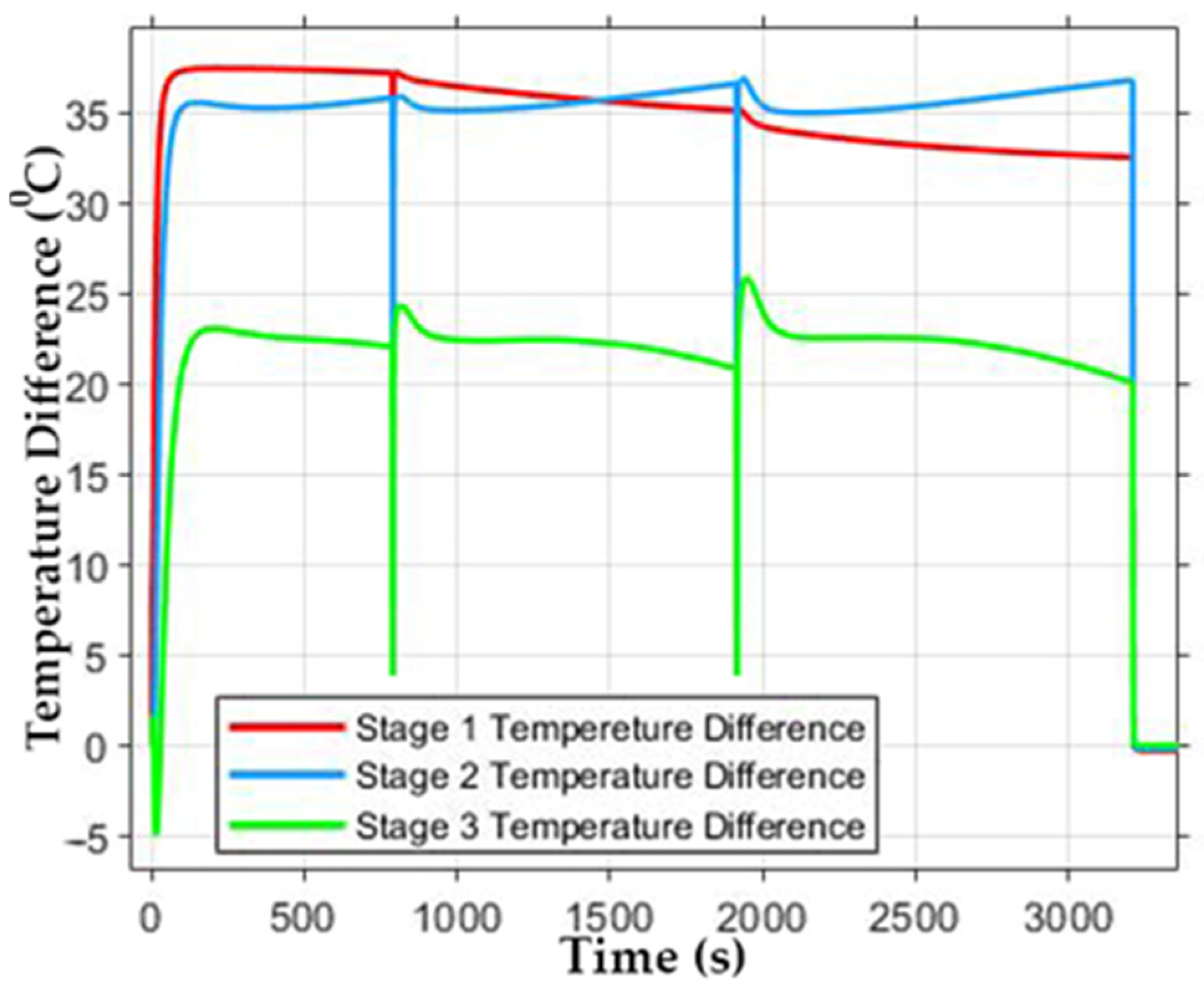
After each compression stage, the natural gas is cooled with water using an intercooler. The temperature difference before and after intercooling is shown in Figure 8. The intercooler reduces the gas temperature by an average of 35 °C at the exit during the first and second stages and by approximately 22 °C at the end of the third stage.

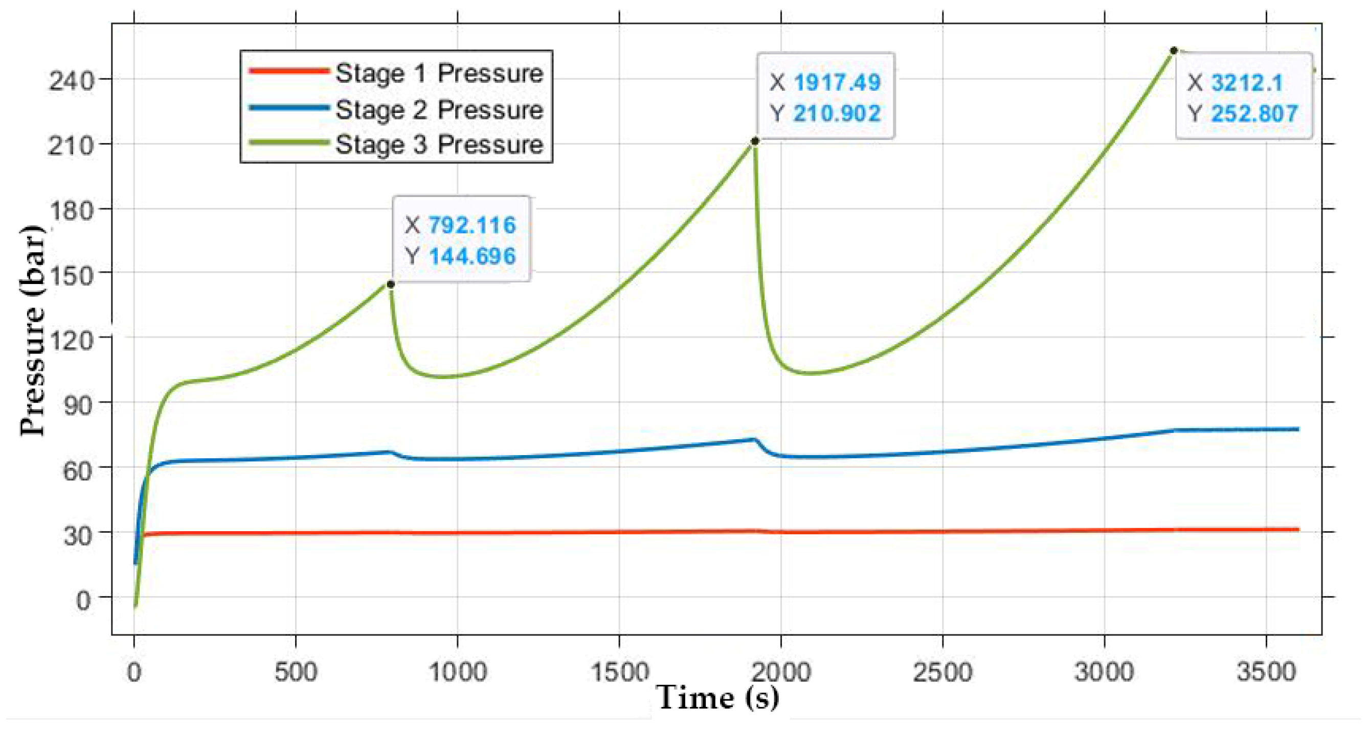
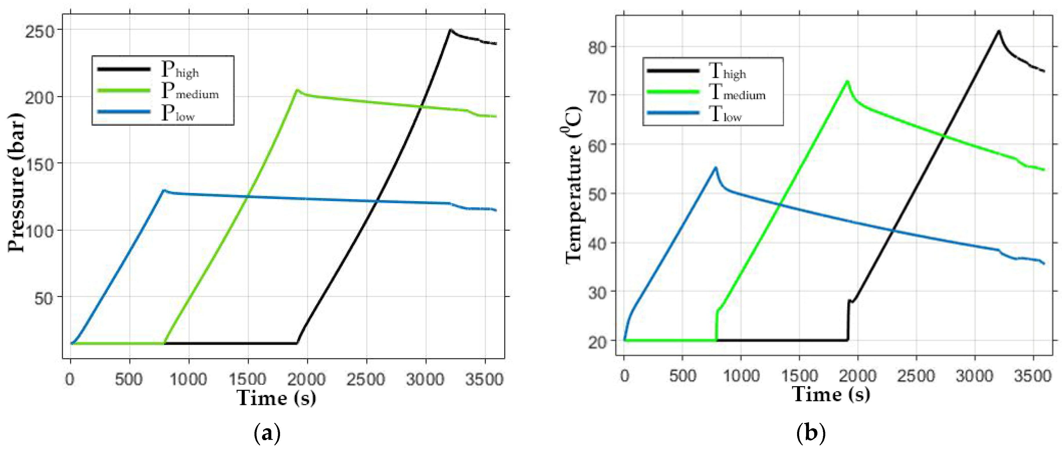
The equal-volume storage tanks take approximately 54 min (3211 s) to reach the set pressure. The filling times for each tank are as follows: LP takes 13 min, MP 19 min, and HP 22 min. The pressure and temperature variations during the filling process are illustrated in Figure 9a,b.

During the filling process, the storage tank temperatures rise, with the LP tank reaching 55 °C, the MP tank 73 °C, and the HP tank 82 °C. Once filling is complete, heat dissipates into the surrounding ambient air, which is at 20 °C, gradually lowering these temperatures.

The 24 h monitoring period begins with the compressor filling the empty storage tanks. Once the tanks reach full capacity, the compressor shuts down and the vehicle tanks are refueled using a dispenser. Three vehicle tanks are selected for this process. While one vehicle tank is being filled, the other two are discharged and reset to an initial pressure of 5 bar at ambient temperature. The total number of vehicle tanks filled within the 24 h period is recorded.

The vehicle tank filling process follows a staged approach. It begins with LP, which initiates the transfer. As soon as the pressure difference between LP and the vehicle tank reaches 10 bar, MP is activated to continue the process. Once MP reaches the same 10 bar pressure difference with the vehicle tank, HP takes over and completes the filling process, bringing the vehicle tank pressure up to 200 bar. After each vehicle tank is filled, the system waits approximately 60 s before initiating the next filling cycle.

The 10 bar pressure difference between the storage tanks was chosen as a design parameter to ensure a sufficient mass flow rate is maintained throughout each phase of the filling sequence. This value is not a fixed standard and may vary depending on station layout, storage tank configuration, and operating objectives. In this study, it was selected to guarantee continuous flow without stagnation, particularly during the high-demand fast-fill process. The model allows this threshold to be easily modified, enabling its application to various design or operational scenarios.

During refueling, LP is excluded from the process if its pressure drops to 55 bar, and MP is excluded when it falls to 130 bar. At this point, the next stage begins. If HP drops to 205 bar, the compressor is activated to refill all storage tanks in sequence, starting with LP, followed by MP, and finally HP.

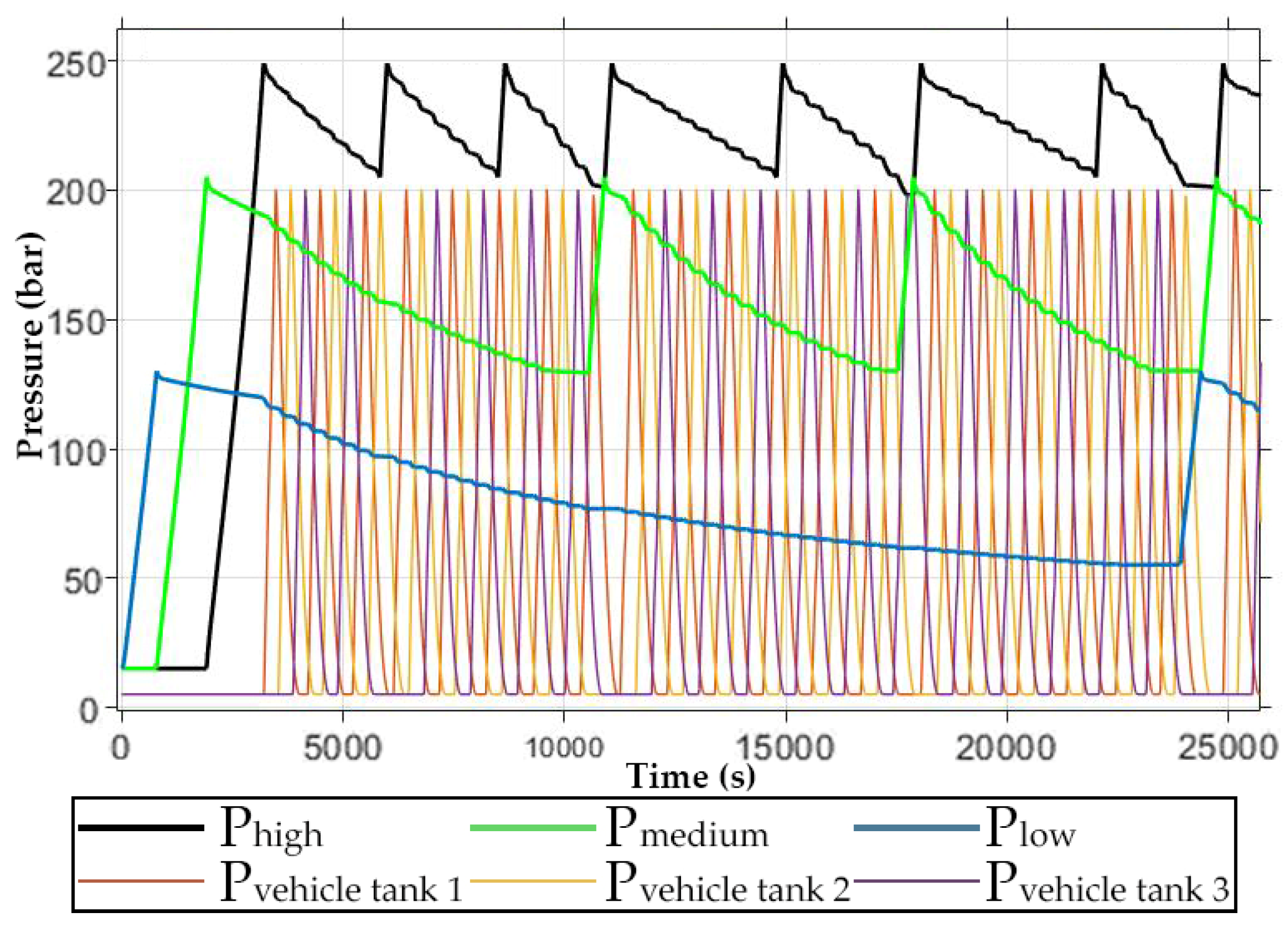
The pressure variations within the system follow a specific range. LP and MP operate with a pressure range of 75 bar, while HP operates within a 45 bar range. On average, the compressor is activated every 60 min to refill HP, while MP and LP require activation every 130 min and 375 min, respectively. The refill times for each storage tank differ, with HP taking 3 min, MP taking 6 min, and LP requiring 9 min to reach full capacity.

Figure 10 illustrates the pressure fluctuations of HP, MP, LP, and the vehicle tanks over a seven-hour period.

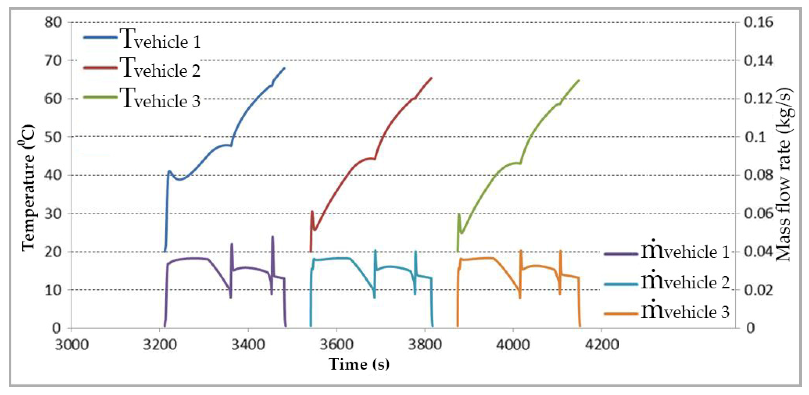
The temperature and mass flow rate variations for the first three vehicle tanks filled are shown in Figure 11. Each vehicle tank is filled in approximately 270 s. Since the storage tanks are newly filled, they are at their maximum pressure and temperature, leading to a higher initial temperature during the first vehicle tank’s filling process.

During filling, the temperature increase in the first three vehicle tanks is 68 °C, 65 °C, and 62 °C, respectively. In subsequent fillings, this temperature rise stabilizes at around 50 °C. The filling times for LP, MP, and HP are 140, 90, and 40 s on average. As the pressures in LP and MP decrease over time, the filling duration of HP increases to compensate.

Flow rate fluctuations occur in the vehicle tanks during the transition between storage tanks. These fluctuations are most noticeable when the mass flow rate drops below 0.02 kg/s. During these transitions, a temperature drop is observed due to the cooling effect.

3.1. Storage Tank Pressure Optimization

After 24 h of monitoring, the compressor was activated four times to refill LP, twelve times for MP, and twenty-four times for HP. A total of 218 vehicle tanks were filled, with an average mass of 9.46 kg per tank. The work performed by the compressor for compression was calculated as 0.1938 kWh per unit mass.

These results indicate that optimizing the selected pressures and volumes of the storage tanks can enhance refueling efficiency. To achieve this, the Taguchi design method was used to analyze the pressure and volume ratios that maximize the number of vehicle tanks filled and the total mass delivered while minimizing compressor operation.

The control factors and levels used in the analysis are presented in Table 4. In the Taguchi design, three control factors were selected to determine storage tank pressures: high storage tank pressure (P_high), medium storage tank pressure (P_medium), and low storage tank pressure (P_low). Each factor had four levels (4³ combinations). The control factor levels were assigned according to the L16 orthogonal array.

For these 16 test cases, the number of vehicle tanks filled in 24 h (n_Vehicle), the average mass of gas accumulated in each vehicle tank (m_average), and the work performed by the compressor per unit mass (W_comp) were calculated. The results are summarized under the “Results” column in

Table 6. Results and S/N ratios according to the L16 orthogonal array.

	Control Factors and Levels			Results			S/N Ratio
Sim. No	Phigh [Bar]	Pmedium [Bar]	Plow [Bar]	nVehicle	mAverage [kg]	WComp [kWh/kg]	nVehicle	mAverage [kg]	WComp [kWh/kg]
1	250	205	130	218	9.46	0.1938	46.77	19.52	14.25
2	250	185	110	214	9.43	0.1946	46.61	19.49	14.22
3	250	165	90	221	9.41	0.1887	46.89	19.47	14.49
4	250	145	70	229	9.43	0.1898	47.20	19.49	14.43
5	240	205	110	217	9.43	0.1910	46.73	19.49	14.38
6	240	185	130	219	9.41	0.1879	46.81	19.48	14.52
7	240	165	70	217	9.36	0.1930	46.73	19.43	14.29
8	240	145	90	217	9.43	0.1881	46.73	19.49	14.51
9	230	205	90	214	9.42	0.1875	46.61	19.48	14.54
10	230	185	70	220	9.39	0.1898	46.85	19.46	14.43
11	230	165	130	213	9.41	0.1923	46.57	19.47	14.32
12	230	145	110	216	9.40	0.1859	46.69	19.46	14.61
13	220	205	70	216	9.41	0.1904	46.69	19.47	14.41
14	220	185	90	210	9.42	0.1862	46.44	19.48	14.60
15	220	165	110	218	9.39	0.1835	46.77	19.45	14.73
16	220	145	130	221	9.39	0.1856	46.89	19.45	14.63

.

Using Minitab software, signal-to-noise (S/N) ratios were computed. The “larger is better” approach was applied to n_Vehicle and m_average, while the “smaller is better” approach was used for W_comp. The calculated S/N ratio values for each output parameter are also provided in Table 6.

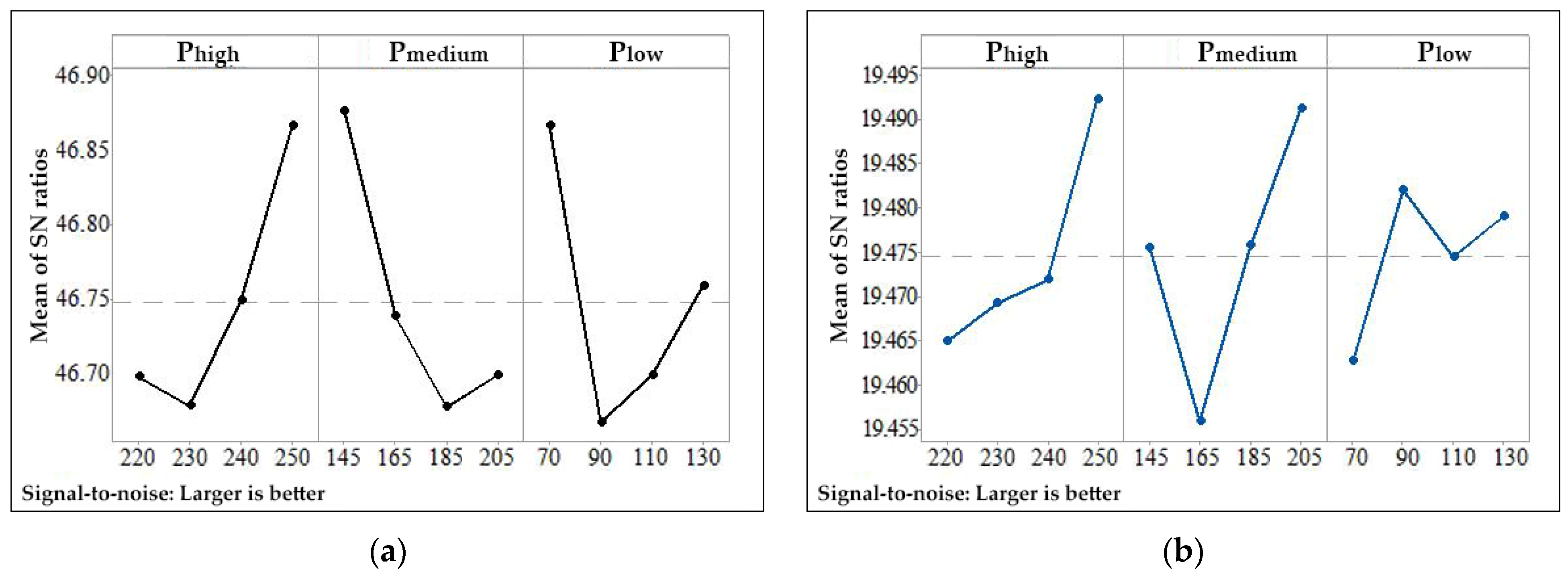
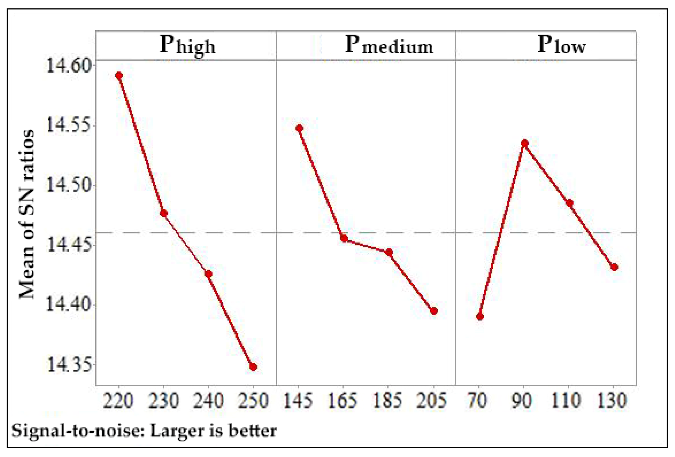
Figure 12a illustrates the calculated S/N ratios for n_Vehicle at specified control factor levels. Optimal performance is achieved by selecting the level that maximizes the S/N value for each factor. The highest n_Vehicle value of 229 occurs when the HP pressure (P_high) is set to 250 bar, the MP pressure (P_medium) to 145 bar, and the LP pressure (P_low) to 70 bar.

Figure 12b presents the S/N ratios of control factors for the average gas mass (m_Average) accumulated in the vehicle tank. The highest m_average value of 9.43 kg is obtained when P_high is 250 bar, P_medium is 205 bar, and P_low is 90 bar. At 130 bar (P_low), which is the second-best option, m_Average is calculated as 9.46 kg.

Figure 13 displays the graphical S/N ratios of control factors for the work performed by the compressor per unit mass filled (W_Comp). The lowest W_Comp value of 0.1898 kWh/kg is achieved when P_high is set to 220 bar, P_medium to 145 bar, and P_low to 90 bar, which correspond to the levels yielding the maximum S/N ratio.

Table 7. The S/N ratios and the weight factors calculated for the n_Vehicle, m_Average, and W_Comp. during storage pressure optimization.

Level	Phigh [Bar]	Pmedium [Bar]	Plow [Bar]
nVehicle
1	46.7	46.88	46.87
2	46.68	46.74	46.67
3	46.75	46.68	46.7
4	46.87	46.7	46.76
Delta	0.1871	0.1982	0.1984
Rank	3	2	1
∑ Delta	0.5837
w (%)	48.82
mAverage [kg]
1	19.46	19.48	19.46
2	19.47	19.46	19.48
3	19.47	19.48	19.47
4	19.49	19.49	19.48
Delta	0.0274	0.0353	0.0192
Rank	2	1	3
∑ Delta	0.0819
w (%)	6.85
WComp [kWh/kg]
1	14.59	14.55	14.39
2	14.48	14.45	14.53
3	14.42	14.44	14.49
4	14.35	14.4	14.43
Delta	0.24	0.15	0.14
Rank	1	2	3
∑ Delta	0.53
w (%)	44.33

presents the calculated S/N ratios of control factors at the levels determined through the Taguchi analysis. The difference between the highest and lowest S/N values for each factor, known as the Delta value, indicates the factor’s influence on the output parameter—a higher Delta signifies a greater impact.

As shown in the table, the Delta values for n_Vehicle are very close. The P_low factor has the highest influence (Delta = 0.1984), followed by P_medium (Delta = 0.1982) and P_high (Delta = 0.1871). Over a 24 h period, P_low and P_medium pressures have a greater effect on the number of vehicles filled than P_high pressure. The ranking in the table reflects the relative importance of each control factor in determining the number of vehicles filled within this period. The weighting coefficient for n_Vehicle is w = 48.82%.

The impact of control factors on the average filled gas mass (m_Average) was also analyzed using the Taguchi method, with results shown under the m_Average row in Table 7. Here, the Delta values are even smaller, indicating a lower influence. As a result, the weighting factor for m_average in the multi-objective optimization process is only 6.85%.

Another design objective is minimizing the work performed by the compressor per unit mass filled (W_Comp). The Taguchi analysis confirmed that P_high pressure is the most significant factor in reducing W_Comp, as expected. The influence of W_Comp on the objective function (weighting factor w) is 44.33%.

Since the output parameters examined separately indicated different influential factors, they were integrated based on their respective weights and combined into a single objective function. The Taguchi–gray relational analysis method was employed to generate and analyze this function. The weighting coefficients used in the multi-objective optimization process were derived from the normalized Delta values presented in Table 7. These values represent the sensitivity of each output parameter to the control factors and were used to objectively assign relative importance. Although the entropy weight method was not explicitly applied, this approach serves a similar function by quantifying the information contribution of each response variable in a consistent, data driven manner.

In this approach, the three output parameters listed under the “Results” column, calculated according to the orthogonal array in Table 6, are first normalized using Equations (7) and (8). The normalized results are then presented in

Table 8. Normalization, gray relational coefficient, gray relational grade, and order of output parameters during storage pressure optimization.

	Normalization			Gray Relational Coefficient			GRG	Order
Sim. No	nVehicle	mAverage	WComp	nVehicle	mAverage	WComp
1	0.42	1.00	0.07	0.46	1.00	0.35	0.45	11
2	0.21	0.68	0	0.39	0.61	0.33	0.38	16
3	0.58	0.45	0.53	0.54	0.48	0.52	0.53	5
4	1.00	0.74	0.43	1.00	0.65	0.47	0.74	1
5	0.37	0.70	0.33	0.44	0.62	0.43	0.45	12
6	0.47	0.53	0.60	0.49	0.51	0.56	0.52	6
7	0.37	0	0.14	0.44	0.33	0.37	0.40	14
8	0.37	0.72	0.58	0.44	0.64	0.54	0.50	7
9	0.21	0.63	0.64	0.39	0.58	0.58	0.49	10
10	0.53	0.32	0.43	0.51	0.42	0.47	0.49	9
11	0.16	0.48	0.20	0.37	0.49	0.39	0.39	15
12	0.32	0.39	0.78	0.42	0.45	0.70	0.55	4
13	0.32	0.48	0.38	0.42	0.49	0.45	0.44	13
14	0	0.59	0.76	0.33	0.55	0.67	0.50	8
15	0.42	0.30	1.00	0.46	0.42	1.00	0.70	2
16	0.58	0.26	0.81	0.54	0.40	0.73	0.62	3

. Next, these values are applied to Equations (9)–(12) to compute the gray relational coefficient (GRC) for each output parameter. Finally, the gray relational grade (GRG) is determined using Equation (13).

The weighting factors calculated for each output parameter, as shown in Table 7, are taken into account, leading to the formulation of the objective function given in Equation (15).

$$\mathrm{GRG}=0{.4882 \mathrm{GRC}}_{{\mathrm{n}}_{\mathrm{Vehicle}}}+0{.0685 \mathrm{GRC}}_{{\mathrm{m}}_{\mathrm{Average}}}+0{.4433 \mathrm{GRC}}_{{\mathrm{W}}_{\mathrm{Comp}}}$$

(15)

The last column of Table 8 ranks the calculated GRG values. Based on these rankings, the optimal result, which represents the simulation design that maximizes the objective function, is achieved with 250 bar (P_high), 145 bar (P_medium), and 70 bar (P_low), corresponding to simulation 4. As a result, the number of vehicle tanks that can be filled in 24 h is n_Vehicle = 229, with an average gas mass of m_Average = 9.43 kg, and the compressor’s work per mass filled is W_Comp = 0.1898 kWh/kg.

Taguchi analysis was conducted to assess the influence of control factors on the obtained GRG, with the results presented in

Table 9. S/N ratios of the gray relational grade.

Level	Phigh	Pmedium	Plow
1	−5.137	−4.521	−5.996
2	−6.512	−6.218	−5.966
3	−6.65	−6.598	−5.951
4	−5.886	−6.847	−6.273
Delta	1.513	2.326	0.322
Rank	2	1	3

. Analyzing the Delta and Rank values in the table reveals that the parameters influencing the objective function the most are P_medium, followed by P_high and P_low.

3.2. Storage Tank Volume Optimization

Up to this point in the study, the volumes of the three storage tanks have been assumed to be equal. The Taguchi design was applied once again to evaluate how different volume ratios affect the performance of the fuel station and to determine the optimal ratio. The control factors and their levels used in the analysis are listed in Table 5.

In the Taguchi design, two control factors were selected to define the tank volumes. The first is the ratio of LB volume to total volume (${\overline{\mathrm{v}}}_{\mathrm{low}}$), given in Equation (1). The second is the ratio of MP volume to HP volume (${\overline{\mathrm{v}}}_{\mathrm{m}/\mathrm{h}}$), given in Equation (4), for the remaining volume. Each factor has three levels, resulting in nine cases (3² = 9). These levels are based on a total storage volume of 48 tanks, each with a 150 L capacity, leading to a total of 7200 L. The control factor values are designed to align with the L9 orthogonal array.

For each of the nine cases, the number of vehicle tanks that can be filled in 24 h (n_Vehicle), the average mass of gas accumulated in a vehicle tank (m_Average), and the work performed by the compressor per mass charged (W_Comp), are calculated. In these calculations, the pressure values that yielded the best results in previous analyses are used. The results are summarized in

Table 10. Results and S/N ratios according to L9 orthogonal array.

	Control Factors and Levels		Results			S/N Ratio
Sim. No	${\overline{\mathbf{v}}}_{\mathbf{low}}$	${\overline{\mathbf{v}}}_{\mathbf{m}/\mathbf{h}}$	nVehicle	mAverage [kg]	WComp [kWh/kg]	nVehicle	mAverage [kg]	WComp [kWh/kg]
1	0.25	0.5	231	9.511	0.200	47.272	19.564	13.989
2	0.25	1	227	9.456	0.194	47.121	19.514	14.263
3	0.25	2	229	9.358	0.185	47.197	19.424	14.638
4	0.5	0.5	226	9.335	0.188	47.082	19.402	14.502
5	0.5	1	224	9.290	0.184	47.005	19.360	14.708
6	0.5	2	229	9.209	0.177	47.197	19.284	15.024
7	0.75	0.5	231	9.021	0.175	47.272	19.105	15.127
8	0.75	1	229	8.979	0.173	47.197	19.065	15.262
9	0.75	2	229	8.941	0.170	47.197	19.027	15.413

under the column heading “Results.”

Following this, S/N (signal-to-noise) ratios were calculated using the larger-is-better approach for n_Vehicle and m_Average, while the smaller-is-better approach was applied for W_Comp. The S/N ratio values for each output parameter are also presented in Table 10.

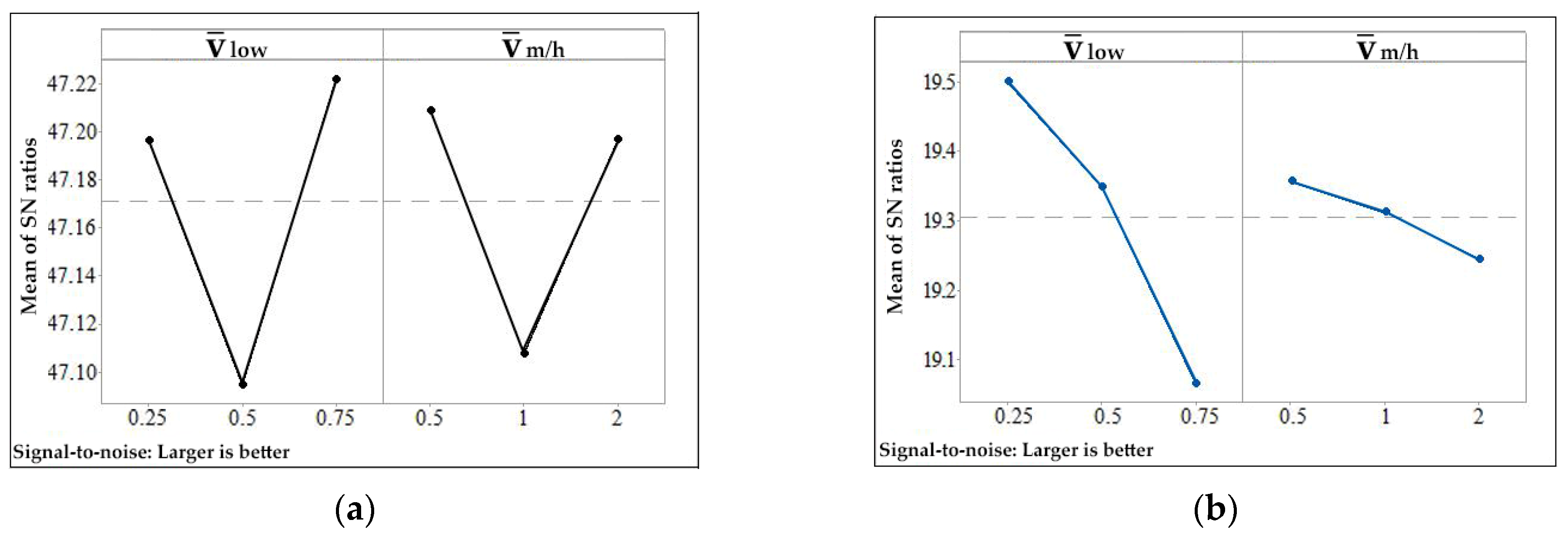
Figure 14a illustrates the behavior of the S/N ratios calculated for n_Vehicle at the specified levels of the control factors. According to this figure, the maximum n_Vehicle of 231 is achieved when the ratio of LB volume to total volume (${\overline{\mathrm{v}}}_{\mathrm{low}}$) is set to 0.25 and the ratio of MP volume to HP volume (${\overline{\mathrm{v}}}_{\mathrm{m}/\mathrm{h}}$) is set to 0.5.

Figure 14b presents the calculated S/N ratios of the control factors for the average gas mass (m_Average) accumulated in the vehicle tank. According to this figure, m_Average is approximately 9.511 kg when ${\overline{\mathrm{v}}}_{\mathrm{low}}$ is set to 0.25 and ${\overline{\mathrm{v}}}_{\mathrm{m}/\mathrm{h}}$ is set to 0.5.

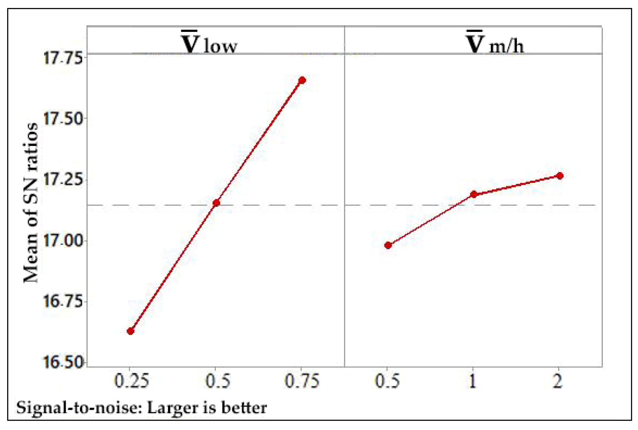
Figure 15 illustrates the graphical representation of the S/N ratios for the control factors calculated for the work performed by the compressor per mass filled (W_Comp). According to this figure, the minimum W_Comp is found to be 0.17 kWh/kg when ${\overline{\mathrm{v}}}_{\mathrm{low}}$ is set to 0.75 and ${\overline{\mathrm{v}}}_{\mathrm{m}/\mathrm{h}}$ is set to 2.

Table 11. The S/N ratios and the weight factors calculated for the n_vehicle, m_Average, and W_Comp.

Level	${\overline{\mathbf{v}}}_{\mathrm{low}}$	${\overline{\mathbf{v}}}_{\mathbf{m}/\mathbf{h}}$
nVehicle
1	47.2	47.21
2	47.09	47.11
3	47.22	47.2
Delta	0.13	0.1
Rank	1	2
∑ Delta	0.23
w (%)	10.31%
mAverage [kg]
1	19.5	19.36
2	19.35	19.31
3	19.07	19.25
Delta	0.43	0.11
Rank	1	2
∑ Delta	0.54
w (%)	24.22%
WComp [kWh/kg]
1	14.3	14.54
2	14.74	14.74
3	15.27	15.02
Delta	0.97	0.49
Rank	1	2
∑ Delta	1.46
w (%)	65.47%

presents the calculated S/N ratios of the control factors at the levels determined through the Taguchi analysis. For the number of vehicle tanks that can be filled in 24 h, the calculated weighting factor for n_Vehicle is 10.31%. The effects of the control parameters on the average mass of gas filled are shown in the m_Average row, with a weighting factor of 24.22% in the multi-objective optimization process. The work performed by the compressor per filled mass (W_Comp) has the highest impact on the objective function, with a weighting factor of 65.47%.

In the Taguchi–gray relational analysis method, the results are first normalized, and the gray relational coefficients are calculated, as shown in

Table 12. Normalization, gray relational coefficient, gray relational grade, and order of output parameters.

	Normalization			Gray Relational Coefficient			GRG	Order
Sim. No	nVehicle	mAverage	WComp	nVehicle	mAverage	WComp
1	1.00	1.00	0	1.00	1.00	0.33	0.56	5
2	0.43	0.90	0.21	0.47	0.84	0.39	0.50	8
3	0.71	0.73	0.48	0.64	0.65	0.49	0.54	6
4	0.29	0.69	0.38	0.41	0.62	0.45	0.48	9
5	0	0.61	0.53	0.33	0.56	0.51	0.51	7
6	0.71	0.47	0.74	0.64	0.49	0.66	0.62	4
7	1.00	0.14	0.81	1.00	0.37	0.73	0.67	3
8	0.71	0.07	0.90	0.64	0.35	0.84	0.70	2
9	0.71	0	1.00	0.64	0.33	1.00	0.80	1

. The gray relational grade (GRG) is then computed using Equation (16), which is derived based on the weighting factors in Table 11. The GRG results obtained from Equation (16) are presented in Table 12, with the final column displaying the ranking of the calculated GRG values.

As a result, the optimal simulation design is achieved with parameters of 0.75 for ${\overline{\mathrm{v}}}_{\mathrm{low}}$ and 2 for ${\overline{\mathrm{v}}}_{\mathrm{m}/\mathrm{h}}$, corresponding to simulation 9. The selected simulation 9 results are: n_Vehicle = 229, m_Average = 8.941 kg, and W_Comp = 0.17 kWh/kg. With this configuration, n_Vehicle increases while W_Comp and m_Average decrease.

$$\mathrm{GRG}=0.1031 {\mathrm{GRC}}_{{\mathrm{n}}_{\mathrm{Vehicle}}}+0.2422 {\mathrm{GRC}}_{{\mathrm{m}}_{\mathrm{Average}}}+0.6547 {\mathrm{GRC}}_{{\mathrm{W}}_{\mathrm{Comp}}}$$

(16)

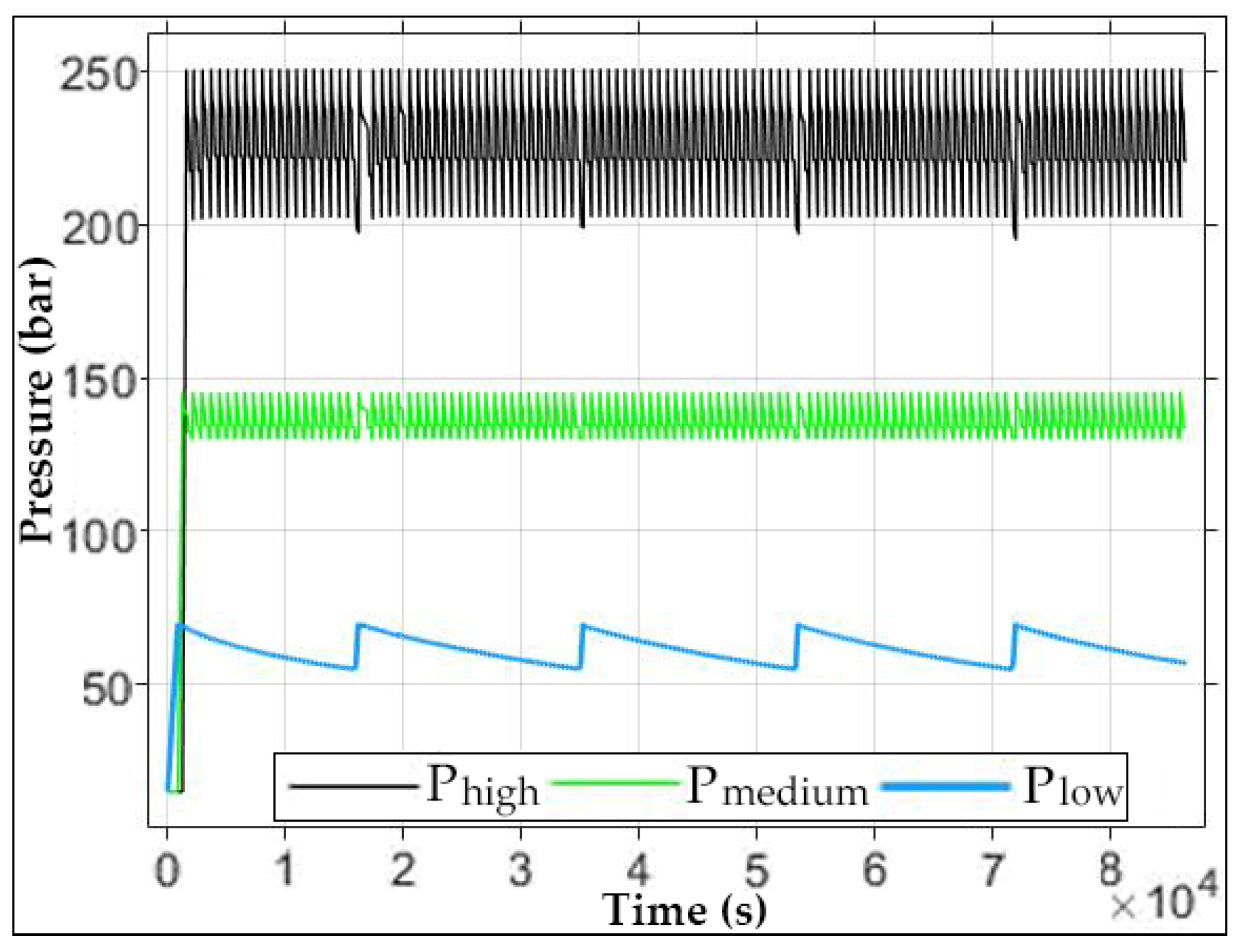
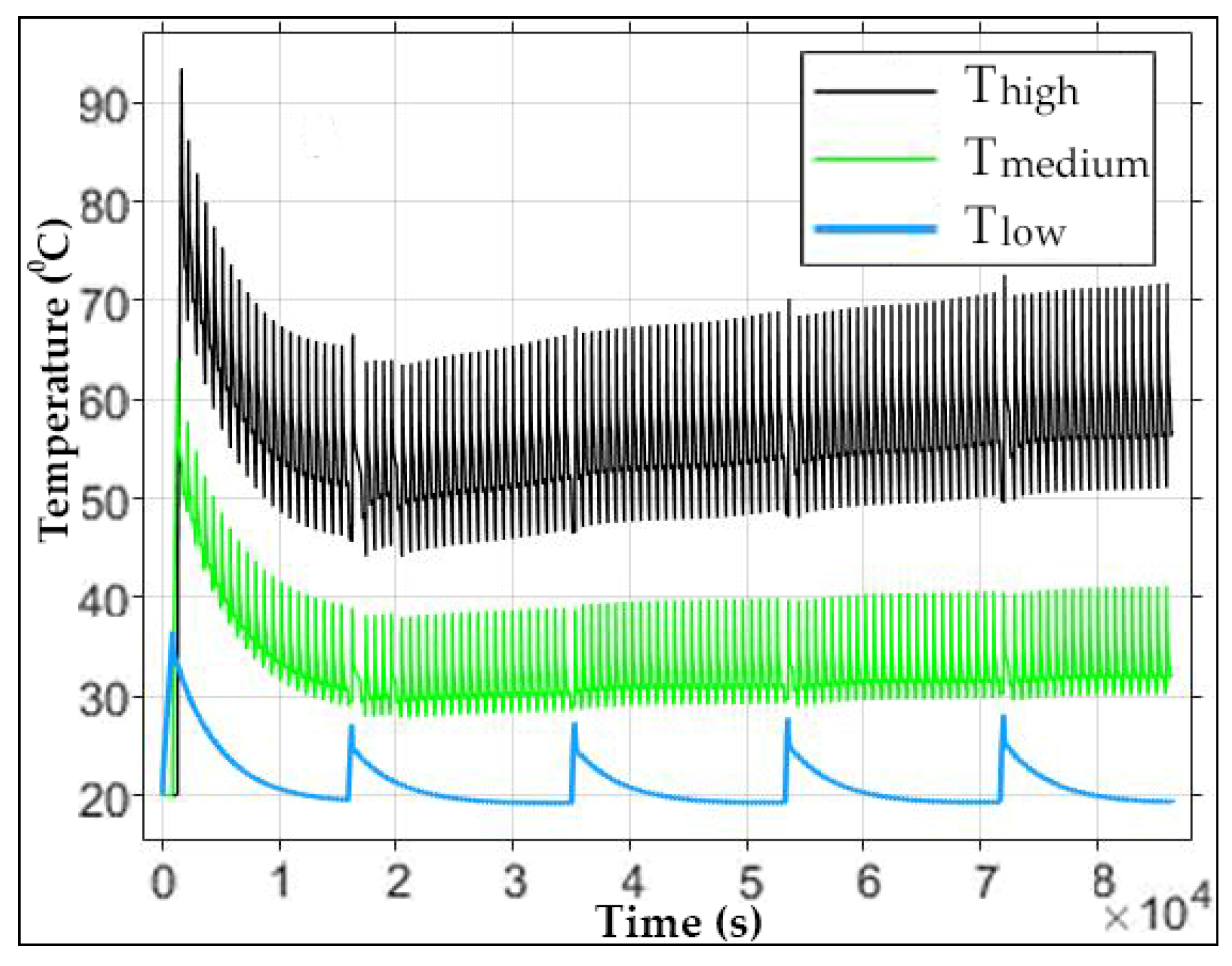
Following the pressure and volume optimizations, the pressure and temperature variations of the storage tanks during a 24 h operation are presented in Figure 16 and Figure 17. The pressure of the high-pressure storage tanks, indicated by the black line, reaches up to 250 bar as a result of the optimization. Since the vehicle tanks are intended to be filled up to 200 bar, the minimum pressure level of the high-pressure storage tanks is set to 205 bar. According to the volume optimization, only 4 out of the total 48 storage tanks are designated as high-pressure tanks. This results in a rapid pressure drop to the minimum level in these tanks, causing the compressor to frequently engage and restore the pressure to its maximum level. In this context, it requires compressor activation roughly every 12.5 min. Due to the frequent and short-term refilling by the compressor, the temperature in the high-pressure storage tanks remains consistently high. During the first filling process, the low-, medium-, and finally high-pressure storage tanks are filled in sequence, leading to the highest temperature being observed during this initial filling phase.

The medium-pressure storage tanks, represented by the green line, reach a maximum pressure of 145 bar as a result of the optimization. To participate in the filling process, their minimum pressure is set to 130 bar. In line with the volume optimization, 8 out of the 48 tanks are assigned as medium-pressure storage tanks. Due to the narrow pressure range and their share of only one-sixth of the total storage volume, these tanks are also refilled by the compressor within short time intervals.

The low-pressure storage tanks, shown by the blue line, have a maximum pressure of 70 bar and a minimum pressure of 55 bar. Similar to the medium-pressure group, the pressure range is relatively narrow. However, based on the volume optimization, three-quarters of the total storage capacity is allocated to the low-pressure tanks. As a result, it takes significantly longer for the pressure in these tanks to drop to the minimum level. Therefore, they need to be refilled only five times during the 24 h period. Due to the lower refilling frequency, their temperature gradually decreases to ambient levels.

Table 13. CNG station performance before optimization, after pressure optimization, and after volume ratio optimization.

Performance Indicator	Initial Configuration	After Pressure Optimization	After Volume Optimization
Number of vehicles refueled (nVehicle)	218	229	229
Average mass per vehicle (mAverage, kg)	9.46	9.43	8.94
Compressor specific work(WComp, kWh/kg)	0.1938	0.1898	0.17

provides a stage-wise summary of CNG station performance before optimization, after pressure optimization, and after volume ratio optimization. It reflects the incremental improvements achieved through each stage of the Taguchi–GRA optimization process.

4. Discussion

This study presents a dynamic modeling and multi-objective optimization of a compressed natural gas (CNG) refueling station. The system model includes the full refueling cycle: multi-stage compression, cascade storage, vehicle tank filling, and thermodynamic interactions. The model was constructed with a modular structure by using a dynamic simulation environment and was validated against experimental data for pressure and mass flow rate profiles.

The effects of varying storage pressures and volume allocations were investigated through a two-stage Taguchi-based optimization framework combined with gray relational analysis (GRA). In the first stage, the optimal storage pressures were determined as 250 bar (P_high), 145 bar (P_medium), and 70 bar (P_low). Compared to the initial configuration, these settings increased the number of vehicles refueled in a 24 h cycle by 5.05%, improved the average charged gas mass by 0.34%, and reduced the compressor specific work by 2.07%.

In the second optimization stage, optimal volume ratios were identified as V_low/V_total = 0.75 and V_medium/V_high = 2. This configuration led to an additional 5.18% reduction in compressor-specific work compared to equal volume tanks, with no significant change in the number of vehicles filled. However, this stage resulted in a 5.5% reduction in the average mass delivered per vehicle, indicating a trade-off between energy efficiency and refueling completeness.

The combined pressure and volume optimization resulted in a total decrease of 12.33% in compressor-specific energy consumption. These findings demonstrate that both pressure levels and volume distributions in cascade storage systems are critical parameters that strongly affect the thermodynamic performance and energy requirements of CNG stations. The applied optimization methodology provides a systematic approach for evaluating such multi-parameter systems under transient operation.

In the Taguchi analysis stage, the main effects of each input factor on system response variables were independently examined. For example, increasing the initial pressure in the high pressure section of the cascade storage system resulted in a higher average refueling mass due to the greater pressure differential, but it also increased energy consumption due to the additional compressor workload. In the subsequent GRA stage, where multi-objective optimization was performed, the trade-off between energy savings and filling performance became more apparent. In particular, activating the priority valve earlier in the filling cycle improved energy efficiency while causing a slight decrease in the amount of gas transferred to vehicle tanks. These results can be physically explained by the pressure driven gas flow and the thermodynamic behavior of real gas during rapid compression and expansion. Therefore, the optimization process revealed the engineering balance required between performance objectives and system level physical behavior. These findings are supported by the performance comparison presented in Table 13, and they are consistent with the physical mechanisms described in the literature [24,27].

In terms of practical applications, the optimized pressure levels and volume ratios obtained in this study can serve as a guideline for designing more efficient cascade storage configurations in real world CNG refueling stations. These configurations may reduce the workload on compressors, enhance the consistency of fuel delivery, and improve operational energy efficiency. For future work, it is recommended to implement adaptive control strategies that can respond to varying demand profiles and to compare the current Taguchi–GRA optimization framework with other multi-objective approaches, such as NSGA-II or Particle Swarm Optimization (PSO), to evaluate performance under more complex operational conditions.