Determination of the Spring Constant for the Horizontal Movement of Rigid Rectangular Foundations Resting on Elastic Subsoil

Abstract

In this paper, a formula for the spring constant $K_x$ for the horizontal movement of rigid rectangular foundations resting on elastic subsoil and spring coefficient ${\beta }_x$ in this formula was derived, which demonstrates that ${\beta }_x$ depends on Poisson’s ratio ν. It was also shown that ${\beta }_x$, which has already been presented in the literature, was determined for a constant value ν = 0.3. It was shown that the values of ${\beta }_x$ and $K_x$, obtained from the formulas derived in this paper and the calculations based on the formulas and nomogram for the ${\beta }_x$ given in the literature, may differ by 8–11%. For the adopted parameters, among others ν = 0.5, and for the side ratio α = 10, the value of spring constant is in the first case $K_x=1$45.9 MN/m and in the second case $K_x$ = 158.3 MN/m (differ by 8%), while for ν = 0.1, is, respectively, $K_x$ = 517.8 N/m and $K_x$ = 464.3 MN/m (differ by 11%). Numerical FEM 3D analysis verified analytical solutions for the concrete foundation footing and the soil layer beneath it. This paper also provides useful nomograms that can be used to easily read the values $K_x$ and ${\beta }_x$. The use of the proposed formulas in this paper, refined formulas for determining $K_x$and ${\beta }_x$ in engineering calculations, can improve the accuracy of the analyses related to the influence of soil stiffness in horizontal movement.

1. Introduction

In the case of building structures (buildings, bridges, retaining walls, masts, etc.) that transfer their loads to the ground via foundations, deformations of the subsoil must be taken into account. When designing foundations of any type, including isolated footings, strip wall footings, slabs, or piles, it is very important to prevent excessive settlements that could damage the structure or reduce its utility value. Nowadays, in the era of using technologically advanced software and computers, taking into account a number of factors that significantly affect the deformation of a structure in the calculation models is not a problem for a structural engineer [1,2]. Nevertheless, the time needed to perform such calculations is often significantly extended (up to several or even a dozen or so hours). Therefore, a simplified structure scheme and a typical method of support are still often used for the structural and dynamic calculations of building structures.

In engineering calculations, the support of a structure is often assumed in the form of fixed, hinged, or pinned supports, which allow for free movement along a specific direction or a specific surface. With such assumptions, the structure itself is treated as a deformable body, and the supports as being rigidly connected to a non-deformable medium. The adoption of such a simplified method of modeling any support of a structure can cause significant differences between the results obtained from structural calculations and the work of the actual structure. This, in turn, can have an impact on the uneconomical design of structures.

A very often adopted model of elastic subsoil in engineering calculations is the Winkler model [3], in which it is assumed that the settlement w at any point in the ground is directly proportional to the pressure p applied at this point, i.e., p = K·w. The settlement of a given point only depends on the pressure applied at this point and is completely independent of the pressures acting in the vicinity. It is, therefore, a set of springs that are not connected to each other. The K coefficient is called the modulus of subgrade reaction. This is a so-called one-parameter model.

In the literature, there are the so-called two-parameter models, which better describe the actual behavior of the soil under a foundation, i.e., they take into account soil deformations that often occur at a considerable distance from the acting loads. In these models, structural elements are introduced that connect single elastic bonds and ensure their mutual cooperation. Two-parameter models were proposed by, among others: Pasternak [4], Kerr [5], Filonienko-Borodich [6], Muravsky [7], and Świtka [8]. In the first three models, the additional structural elements include an incompressible layer subjected to shear, a shearing layer placed between two spring layers with different elasticity characteristics, a tensile tendon (for a one-dimensional problem), or a tensile membrane (for a two-dimensional problem). In the last two models, the cooperation of individual springs, which are connected to each other by additional springs that have different stiffness characteristics, was assumed.

For many years, elastic half-space has been considered and adopted in the literature for calculations. In such a space, soil is treated as a continuous, homogeneous, and elastic body of infinitely large dimensions, which is limited on one side by a half-plane. In such a model, there is an assumption that the soil can be treated as an environment to which, under certain conditions, the formulas of the elasticity theory can be applied. According to this theory, the elastic properties of the soil are characterized by Young’s modulus of soil E and Poisson’s ratio ν. As studies have shown, this theory allows for a sufficiently accurate reflection of the actual state and can be applied to both cohesive and non-cohesive soils [9,10,11,12]. However, it is important to properly interpret and estimate soil parameters. In this paper, the plastic state that could appear in the soil in the case of very large loads is omitted—the soil, like any other material, then begins to “flow”. It is assumed that when calculating most structures and foundations on elastic soil, relatively small loads occur on the soil. Therefore, in simpler analyses, the linear–elastic behavior of the soil is acceptable [12].

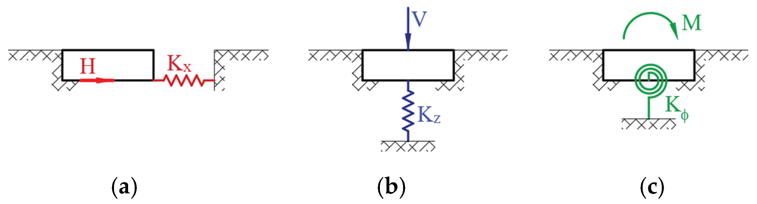
Richart, Woods, and Hall [10]; Whitman and Richart [13]; Lambe and Whitman [11]; and Braja M. Das [14], based on assumptions for the elastic half-space, gave simplified relations for the spring constants of soil. These are, respectively:

-

The soil spring constant $K_x$, which is related to the horizontal movement (see Figure 1a)

$$K_x=2G(1+\nu )\sqrt{A}·{\beta }_x,$$

(1)

-

The soil spring constant $K_z$, which is related to the vertical movement (see Figure 1b)

$$K_z={\displaystyle \frac{G}{1-\nu }}·{\beta }_z\sqrt{A},$$

(2)

-

The soil spring constant $K_{\varphi }$, which is related to the rotational movement (see Figure 1c)

$$K_{\varphi }={\displaystyle \frac{G}{1-\nu }}·{\beta }_{\varphi }·8a{b}^2,$$

(3)

where

• G [Pa]—the shear modulus of soil; ν [-]—the Poisson’s ratio of soil; A [m²]—the foundation area (A = 2a·2b); 2a [m]—the length of the foundation (along the axis of rotation in the case of rocking); 2b [m]—the width of the foundation (in the plane of rotation in the case of rocking); and ${\beta }_x,{\beta }_z,{\beta }_{\varphi }$ [-]—the spring coefficients.

It should be mentioned that when describing the values characterizing the discussed models ($K_x$, $K_z$, and $K_{\varphi }$), the authors cited above call them “constants”, which should be considered imprecise in view of the current knowledge on the nonlinear behavior of the soil medium. However, in order to maintain consistency with the cited literature, this nomenclature was also adopted in this work.

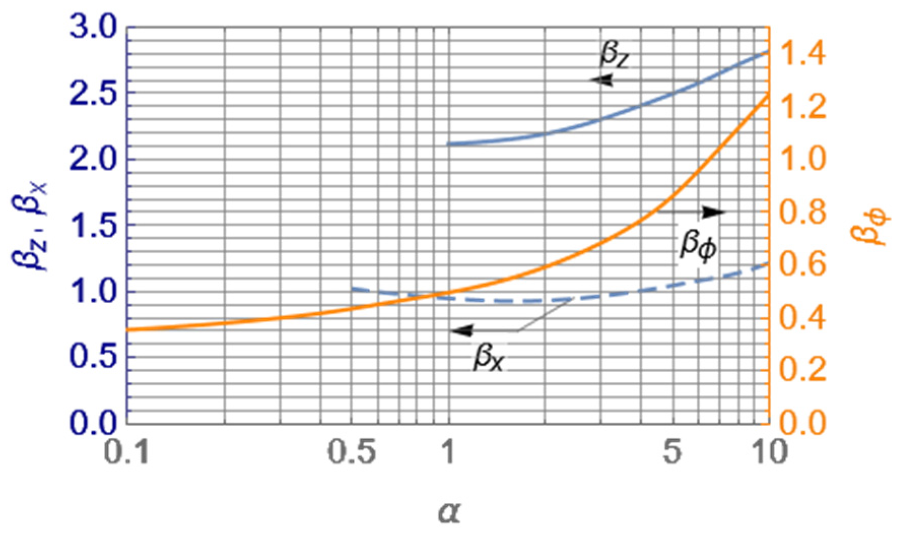
The slab geometry designations are shown in Figure 2. The spring coefficients ${\beta }_x$, ${\beta }_z$, and ${\beta }_{\varphi }$ for a rectangular foundation can be determined from the nomogram in Figure 3.

Richart, Woods, and Hall [10]; Whitman and Richart [13]; Lambe and Whitman [11]; and Braja M. Das [14] reported that the spring constant $K_x$, related to horizontal movement, and the spring constant $K_z$, related to vertical movement, were derived based on the assumptions given in Barkan’s paper [9]. In turn, the spring constant $K_{\varphi }$, which corresponds to rotational movement, was derived based on the assumptions of Gorbunov-Possadov’s papers [12,15]. It should be emphasized that a spring constant represents a linear relationship between the applied load and the foundation displacement, which in turn implies a linear stress–strain relationship of the soil. The formulas for the spring constants were obtained for rigid footings [10]. These formulas are still used to model the contact between the structure and the subsoil and can be found in the source literature [16,17,18,19].

In this paper, based on the assumptions given by Barkan [9], the formula for the spring constant $K_x$ and the spring coefficient ${\beta }_x$ were derived. It was shown that Poisson’s ratio ν not only occurs in the term of the equation for the spring constant $K_x$ before spring coefficient ${\beta }_x$, but also in the spring coefficient. It was also indicated that the graph showing the dependence between the spring coefficient ${\beta }_x$ and $\alpha ={\displaystyle \frac{a}{b}}$, i.e., the ratio of the length and width of a rectangular footing, which is given, among others, in papers [10,11,13,14,16] and was calculated for a constant value of Poisson’s ratio ν = 0.3.

This paper presents calculation results that illustrate the differences in the values of the spring constant $K_x$, which was calculated for the spring coefficient ${\beta }_x$ that was assumed in accordance with papers [10,11,13,14,16] (i.e., calculated for the constant value ν = 0.3) and for ${\beta }_x$ derived in this paper. Useful nomograms were also provided for reading the values of the spring constant $K_x$ with regard to the change in the following parameters: G—the shear modulus of the soil; A—the foundation area (A = 2a·2b); and also for different parameters of ν—Poisson’s ratio of the soil; and $\alpha ={\displaystyle \frac{a}{b}}$—the ratio of the length and width of a rectangular footing.

In order to verify the analytical solutions, a numerical analysis of the complex 3D Finite Element Method (FEM) model of the concrete footing foundation and the subsoil was performed. The interlayer interaction between the top surface of the soil layer and the bottom surface of the foundation footing was modeled in the numerical model. The model considered the friction between the contact surfaces.

2. Formula for the Spring Constant ${\mathit{K}}_{\mathit{x}}$ (Horizontal Motion)

In this chapter, based on the assumptions given by Barkan [9], the formula for the spring constant $K_x$ and dimensionless spring coefficient ${\beta }_x$ are derived. The theoretical foundations used to derive these formulas are also given. The final form of the formula for $K_x$ can be found, among others, in papers [10,11,13,14,16]. However, these works do not provide either the derivation of these relations or the precise theoretical assumptions.

If a horizontal force is applied to the foundation at the level of the contact zone between the foundation base and the ground (see Figure 1a), the foundation will move in the direction of this force. As engineering experience shows, under conditions that exactly correspond to those established for soil compression, it can be assumed that there is a linear relationship between the foundation sliding and the average sliding shearing stress generated along the plane of contact with the foundation base [9], i.e.,

$${\tau }_{av}=c_{\tau }{S}_e^{’},$$

(4)

where

• ${\tau }_{av}$ [Pa]—the average shearing stress in the soil at the plane of contact with the foundation;
• $S_e^{’}$ [m]—the elastic part of the total horizontal sliding of the foundation base under the action of ${\tau }_{av}$.

Barkan [9] assumed $S_e^{’}=S_{av}^{’}$ and stated that the average value of the horizontal sliding along the surface area 2a by 2b equals

$$S_{av}^{’}={\displaystyle \frac{4a}{\pi }}{\displaystyle \frac{1-{\nu }^2}{E}}\left({\displaystyle \frac{1}{\alpha }}{\mathrm{s}\mathrm{i}\mathrm{n}\mathrm{h}}^{-1}\alpha +{\mathrm{s}\mathrm{i}\mathrm{n}\mathrm{h}}^{-1}{\displaystyle \frac{1}{\alpha }}-{\displaystyle \frac{1}{3}}\left[{\displaystyle \frac{1}{{\alpha }^2}}\left(\sqrt{1+{\alpha }^2}-1\right)+\sqrt{1+{\alpha }^2}-\alpha \right]+{\displaystyle \frac{\nu }{1+\nu }}\left\{{\displaystyle \frac{1}{\alpha }}{\mathrm{s}\mathrm{i}\mathrm{n}\mathrm{h}}^{-1}\alpha +{\displaystyle \frac{1}{3}}\left[\sqrt{1+{\alpha }^2}-\alpha -{\displaystyle \frac{2}{{\alpha }^2}}\left(\sqrt{1+{\alpha }^2}-1\right)\right]\right\}\right){\tau }_{av},$$

(5)

where

• $\alpha ={\displaystyle \frac{a}{b}}$ [-]; $E$ [Pa]—Young’s modulus of soil; $\nu$ [-]—Poisson’s ratio.

By substituting ${\tau }_{av}={\displaystyle \frac{H}{A}}$ [${\displaystyle \frac{\mathrm{N}}{{\mathrm{m}}^2}}$] and $a={\displaystyle \frac{1}{2}}\sqrt{A·\alpha }$ [m] (knowing that $A=2a·2b$ [m²]) into Equation (5), and by making minor transformations, the following is obtained:

$${\displaystyle \frac{H}{S_{av}^{’}}}={\displaystyle \frac{E}{1-{\nu }^2}}\sqrt{A}{·k}_{\tau },$$

(6)

where

$$k_{\tau }={\displaystyle \frac{\pi }{2\sqrt{\alpha }\left(\frac{1}{\alpha }{\mathrm{s}\mathrm{i}\mathrm{n}\mathrm{h}}^{-1}\alpha +{\mathrm{s}\mathrm{i}\mathrm{n}\mathrm{h}}^{-1}\frac{1}{\alpha }-\frac{1}{3}\left[\frac{1}{{\alpha }^2}\left(\sqrt{1+{\alpha }^2}-1\right)+\sqrt{1+{\alpha }^2}-\alpha \right]+\frac{\nu }{1+\nu }\left\{\frac{1}{\alpha }{\mathrm{s}\mathrm{i}\mathrm{n}\mathrm{h}}^{-1}\alpha +\frac{1}{3}\left[\sqrt{1+{\alpha }^2}-\alpha -\frac{2}{{\alpha }^2}\left(\sqrt{1+{\alpha }^2}-1\right)\right]\right\}\right)}},$$

(7)

By substituting $E=2G(1+\nu )$ into Equation (6), $K_x$ is obtained

$$K_x={\displaystyle \frac{H}{S_{av}^{’}}}=2G(1+\nu )\sqrt{A}·{\beta }_x,$$

(8)

where

$${\beta }_x={\displaystyle \frac{1}{1-{\nu }^2}}{·k}_{\tau },$$

(9)

The spring constant according to Formula (8) has the dimension [N/m], whereas the spring coefficient (9) is dimensionless. G [Pa] is the shear modulus of soil.

3. Analytical and Numerical Analysis of the Influence of Poisson’s Ratio on the Obtained Results

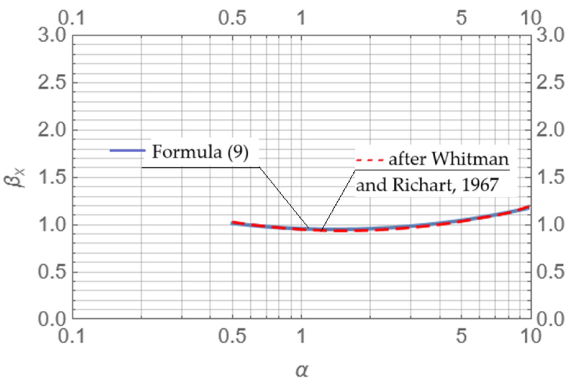
Based on Equation (9), it can be seen that the dimensionless spring coefficient ${\beta }_x$ not only depends on $\alpha ={\displaystyle \frac{a}{b}}$, but also on Poisson’s ratio $\nu$. Additionally, it should be noted that in Formula (8), Poisson’s ratio $\nu$ not only appears in the ${\beta }_x$ coefficient, but also in the term of the equation before this coefficient. In turn, in the literature (among others, in papers [10,11,13,14,16]) the same form of the equation for spring constant $K_x$ as in Equation (8) is given, but the nomogram for reading the ${\beta }_x$ value is only given for one constant value, i.e., $\nu =0.3$ (see Figure 3 and Figure 4). Therefore, a reader wishing to calculate the $K_x$ values based on the formula and nomogram presented in the above-mentioned literature may unknowingly obtain a certain error.

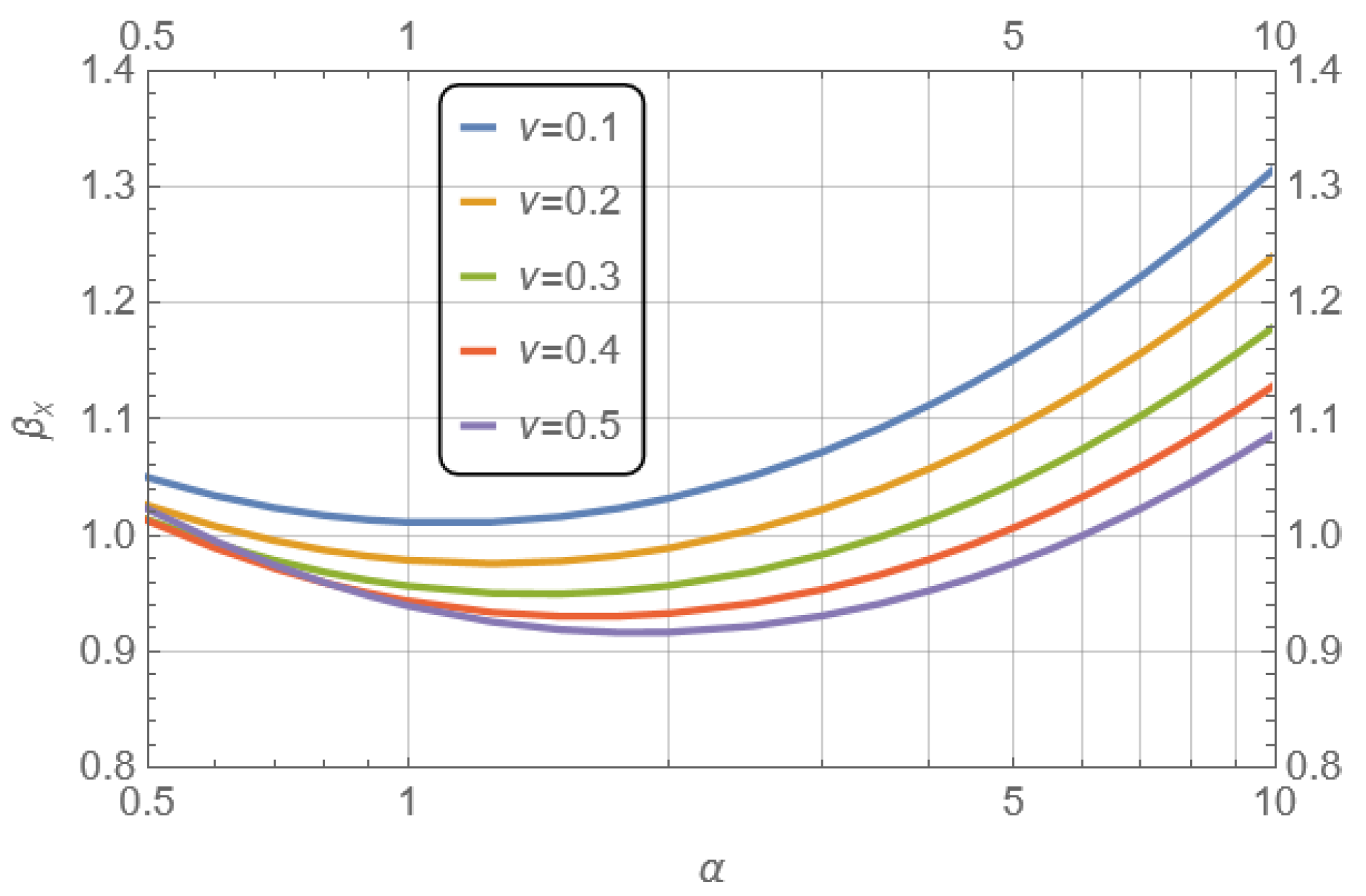
This chapter presents the results of numerical analyses that take into account different values of Poisson’s ratio $\nu ,$ and its influence on both the dimensionless spring coefficient ${\beta }_x$ and the spring constant $K_x$.

In Figure 5 is a nomogram for the dimensionless spring coefficient ${\beta }_x$, plotted for different values of Poisson’s ratio $\nu$, which can be used to more accurately determine the value of $K_x$.

Table 1. Spring coefficient ${\beta }_x$ for rectangular footings with respect to $\alpha ={\displaystyle \frac{a}{b}}$ and Poisson’s ratio $\nu$.

ν	α
	0.5	0.8	1	1.5	2	3	4	5	6	7	8	9	10
0.1	1.050	1.017	1.011	1.016	1.032	1.071	1.112	1.151	1.188	1.223	1.255	1.286	1.316
0.2	1.026	0.987	0.978	0.978	0.989	1.022	1.057	1.092	1.125	1.156	1.186	1.214	1.241
0.3	1.014	0.968	0.956	0.949	0.956	0.983	1.014	1.045	1.074	1.103	1.130	1.155	1.180
0.4	1.013	0.959	0.943	0.930	0.933	0.953	0.979	1.006	1.033	1.059	1.083	1.107	1.129
0.5	1.023	0.959	0.939	0.919	0.917	0.931	0.952	0.976	1.000	1.023	1.045	1.067	1.088

provides the ${\beta }_x$ values for several exemplary values of the $\alpha$ and $\nu$ coefficients.

Table 2. Percentage change in the spring coefficient $\mathsf{\Delta }{\beta }_x$.

ν	α
	0.5	0.8	1	1.5	2	3	4	5	6	7	8	9	10
0.1	3.6%	5.1%	5.8%	7.1%	7.9%	9.0%	9.7%	10.1%	10.6%	10.9%	11.1%	11.3%	11.5%
0.2	1.2%	2.0%	2.3%	3.1%	3.5%	4.0%	4.2%	4.5%	4.7%	4.8%	5.0%	5.1%	5.2%
0.3	0.0%	0.0%	0.0%	0.0%	0.0%	0.0%	0.0%	0.0%	0.0%	0.0%	0.0%	0.0%	0.0%
0.4	−0.1%	−0.9%	−1.4%	−2.0%	−2.4%	−3.1%	−3.5%	−3.7%	−3.8%	−4.0%	−4.2%	−4.2%	−4.3%
0.5	0.9%	−0.9%	−1.8%	−3.2%	−4.1%	−5.3%	−6.1%	−6.6%	−6.9%	−7.3%	−7.5%	−7.6%	−7.8%

shows the percentage change in the spring coefficient ${\beta }_x$ for different values of Poisson’s ratio $\nu$ in relation to the spring coefficient value ${\beta }_x$ calculated at a constant value of $\nu =0.3$. This change was calculated from the following relationship:

$${∆\beta }_x={\displaystyle \frac{{\beta }_x\left(\nu \right)-{\beta }_x\left(\nu =0.3\right)}{{\beta }_x\left(\nu =0.3\right)}}\left[\%\right].$$

(10)

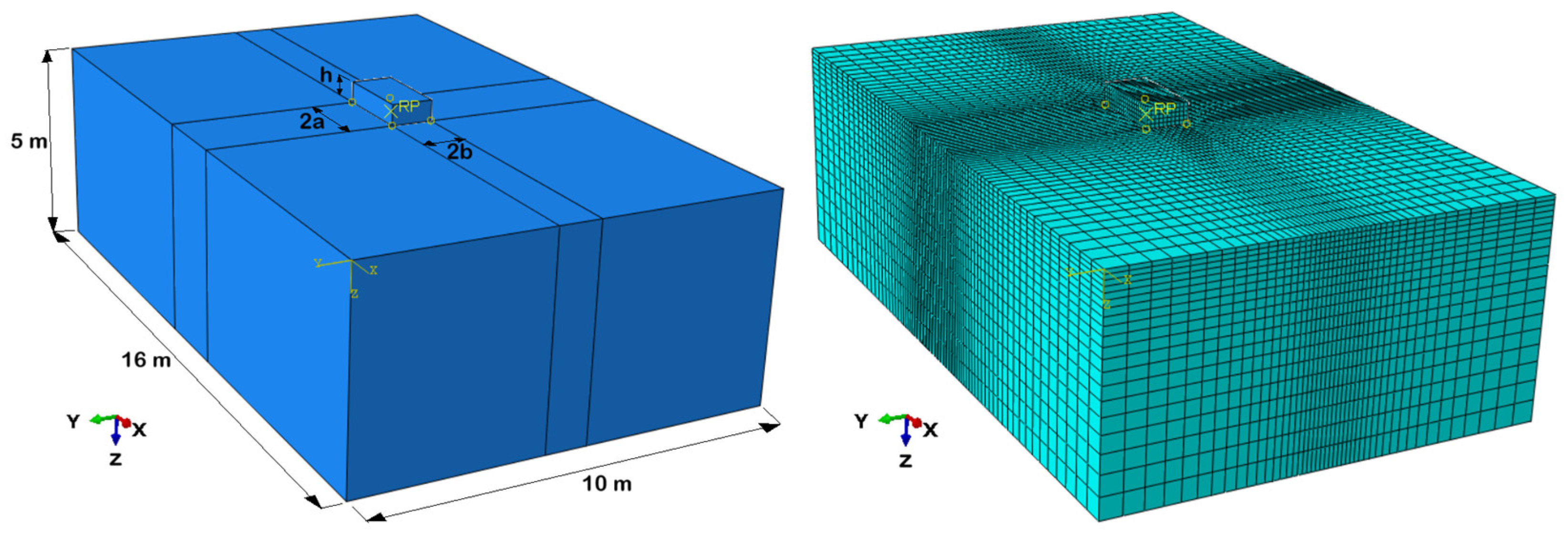
For the purpose of numerically determining the spring coefficient ${\beta }_x$, Finite Element Method (FEM) three-dimensional (3D) models of the concrete foundation footing and the soil (Figure 6) were built using the Abaqus FEA software v. 2017 [20]. The foundation footing and the soil layer beneath it are represented by general-purpose eight-node linear hexahedral elements of type C3D8. The interlayer interaction between the top surface of the soil layer and the bottom surface of the foundation footing was modeled as a standard contact surface-to-surface with friction between the contact surfaces. Furthermore, normal behavior with “hard” contact pressure overclosure and tangential behavior with so-called “rough” friction were used. The adopted contact method permits some relative motion of the contact surfaces after a certain threshold value is exceeded. Due to the nonlinear boundary conditions used in the model, such as contact and friction, the large displacement formulation was used in the static analysis. The self-weight of the soil layer was omitted in the analysis. The following material and geometric parameters were assumed for the calculations:

• Soil: E_s = 100 MPa (Young’s modulus), v = 0.1, 0.2, 0.3, 0.4, 0.5 [-] (Poisson’s ratio),
• Concrete: h = 0.5 m, 2a × 2b = 1 × 1, 2 × 1, 4 × 1, 8 × 1 [m], E_cm = 31 GPa, v = 0.2 [-], ρ = 2400 kg/m³.

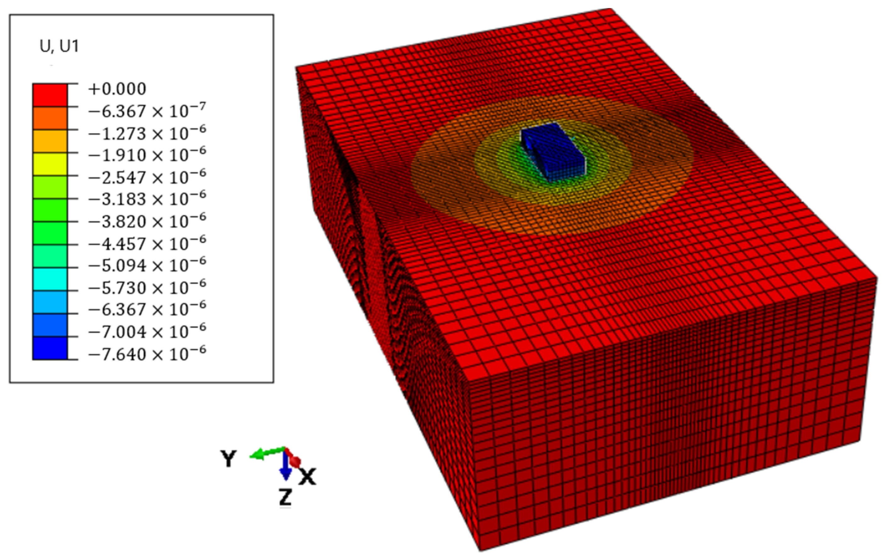
In order to numerically determine the spring coefficient ${\beta }_x$, a horizontal (with respect to the X-axis) unit force was applied to the foundation footing model, which caused displacements (see Figure 7) in the soil and the foundation footing (the base) level. Based on the calculated displacements with respect to the X-axis and the unit force, the spring constant was calculated (see Equation (8)), and then the dimensionless spring coefficient ${\beta }_x$ value (see Equation (9)) was obtained.

Table 3. Spring coefficient ${\beta }_x$ [-] with respect to $\alpha ={\displaystyle \frac{a}{b}}$ [-] and Poisson’s ratio $\nu$ [-] for analytical and numerical calculation.

ν	Analy.	Numer.	Analy.	Numer.	Analy.	Numer.	Analy.	Numer.
	Equation (9)	Abaqus	Equation (9)	Abaqus	Equation (9)	Abaqus	Equation (9)	Abaqus
	α = 1		α = 2		α = 4		α = 8
0.1	1.011	1.043	1.032	1.128	1.112	1.272	1.255	1.519
0.2	0.978	1.034	0.989	1.103	1.057	1.233	1.186	1.468
0.3	0.956	1.043	0.956	1.094	1.014	1.211	1.130	1.435
0.4	0.943	1.077	0.933	1.105	0.979	1.208	1.083	1.423
0.5	0.939	1.163	0.917	1.156	0.952	1.241	1.045	1.450

shows the spring coefficient ${\beta }_x$ with respect to $\alpha ={\displaystyle \frac{a}{b}}$ and Poisson’s ratio ν for analytical and numerical calculations.

Table 4. Percentage change in the spring coefficient $\mathsf{\Delta }{\beta }_x$ [%] for analytical and numerical calculation.

ν	α = 1	α = 2	α = 4	α = 8
0.1	3.0%	8.5%	12.5%	17.4%
0.2	5.4%	10.4%	14.3%	19.2%
0.3	8.4%	12.6%	16.3%	21.3%
0.4	12.4%	15.6%	18.9%	23.9%
0.5	19.2%	20.7%	23.3%	27.9%

shows the percentage change in the spring coefficient ${\beta }_x$. This change was calculated from the following relationship:

$${∆\beta }_x={\displaystyle \frac{{\beta }_x^{Num.}-{\beta }_x^{Anal.}}{{\beta }_x^{Num.}}}\left[\%\right].$$

(11)

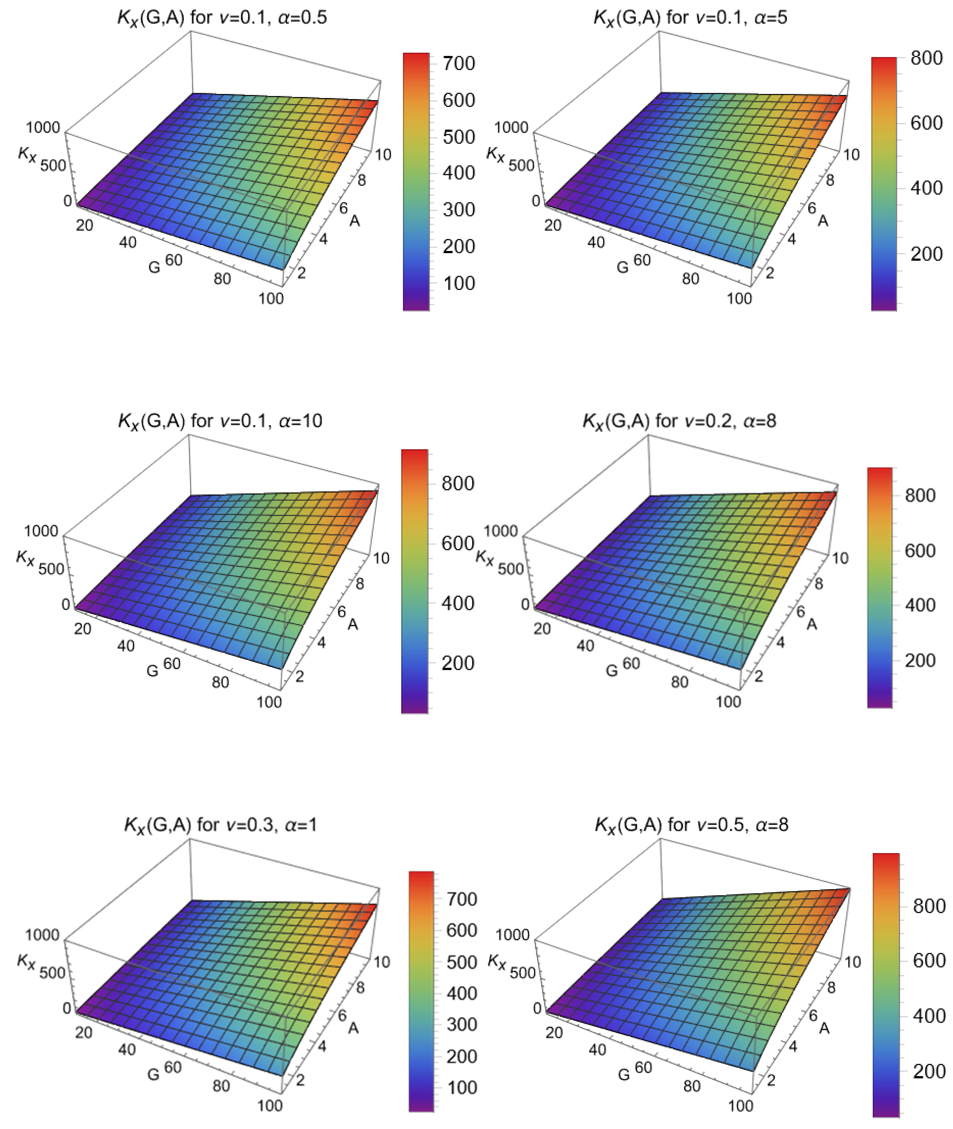
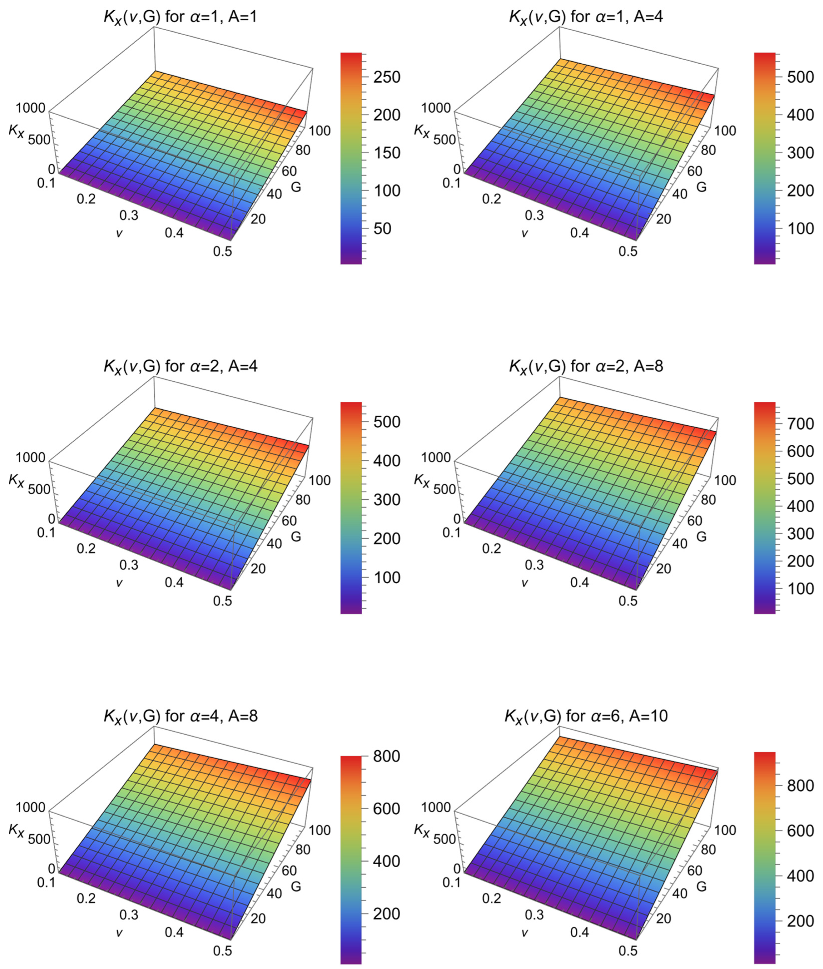
Figure 8 shows the dependence between the spring constant $K_x$ [MN/m] and the shear modulus of soil G [MPa] and the foundation area $A$ [m²] for several different values of $\alpha ={\displaystyle \frac{a}{b}}$ [-] as well as for different Poisson ratios $\nu$ [-]. These solutions were obtained from the analysis of Equation (8).

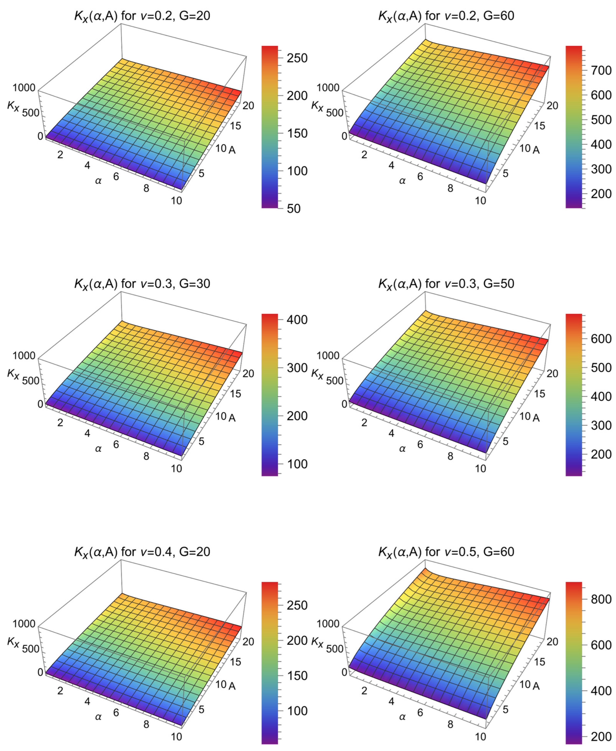
Figure 9 shows the dependence between the spring constant $K_x$ [MN/m] for rectangular footings with respect to the foundation area $A$ [m²] and $\alpha ={\displaystyle \frac{a}{b}}$ [-] for different values of the shear modulus of soil G [MPa] and for different Poisson ratios $\nu$ [-].

Figure 10 shows the dependence between the spring constant $K_x$ [MN/m] for rectangular footings with respect to the shear modulus of soil G [MPa] and the Poisson ratios $\nu$ [-] for different values of the foundation area $A$ [m²] and $\alpha ={\displaystyle \frac{a}{b}}$ [-].

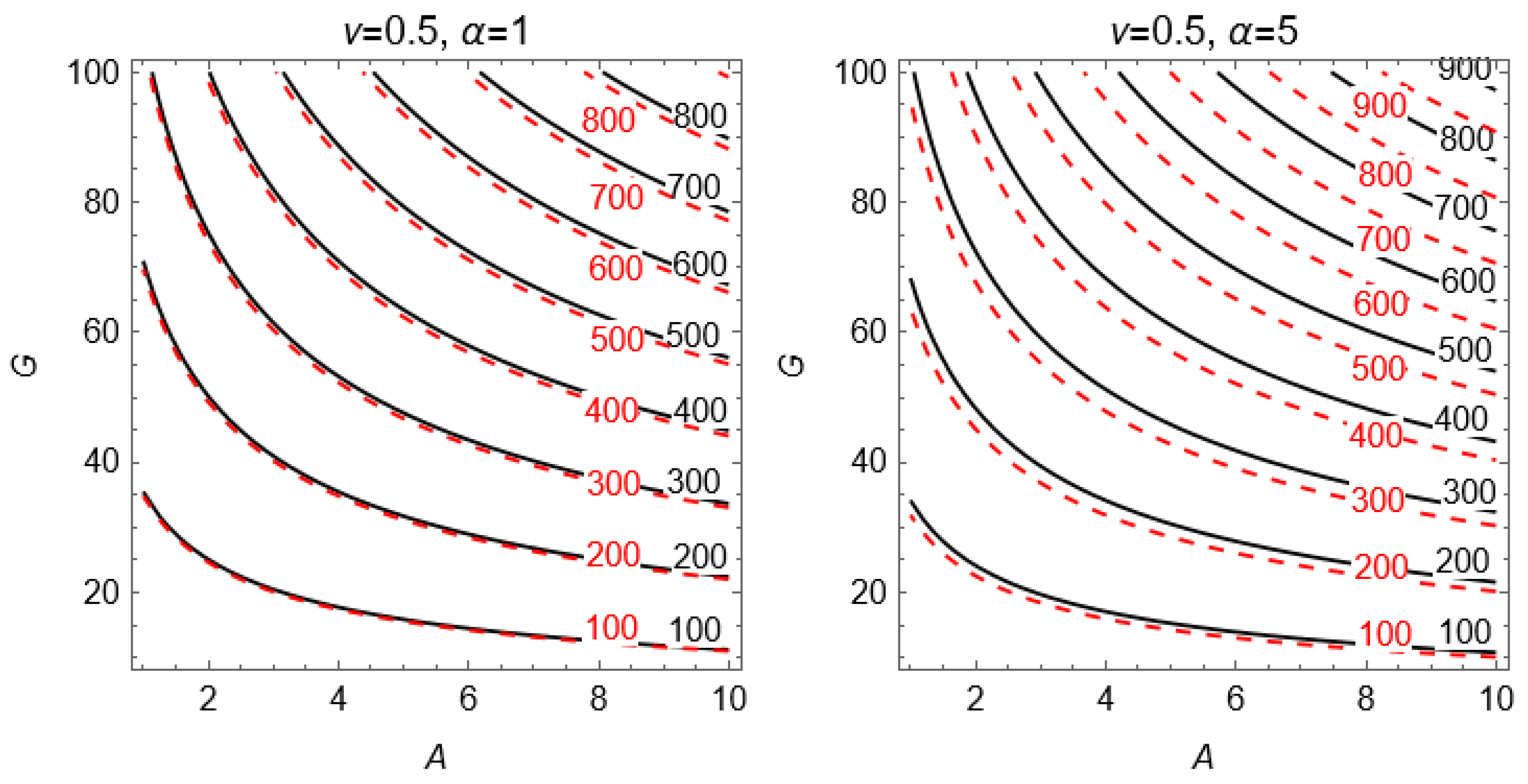
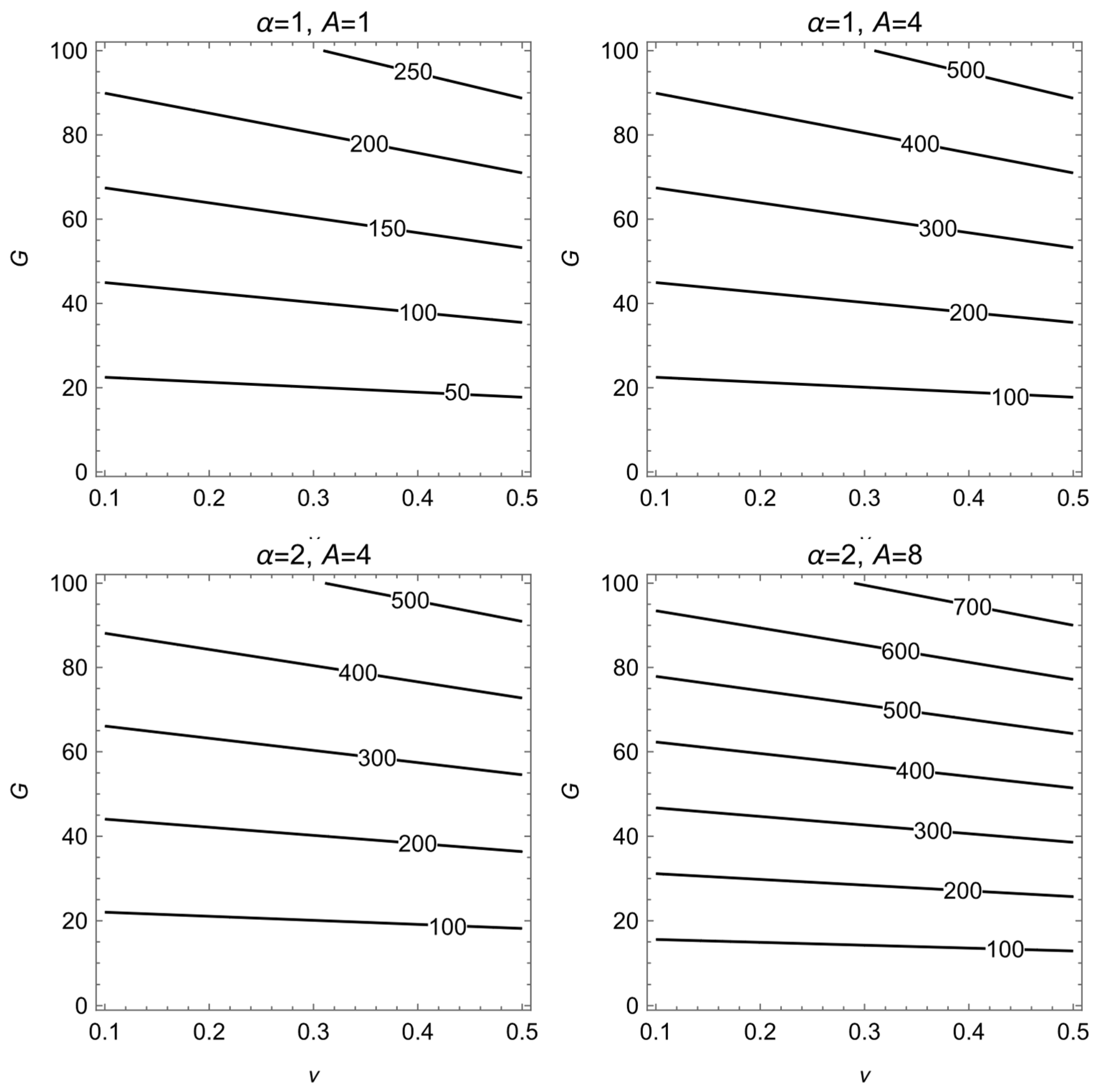
Figure 11 presents contour nomograms showing the values of the spring constant $K_x$[MN/m] with respect to the shear modulus of soil G [MPa] and the foundation area A [m²] for several different values of $\alpha ={\displaystyle \frac{a}{b}}$ [-] and for several different Poisson ratios $\nu$ [-]. The values of the spring constant $K_x$[MN/m] can be easily read from these nomograms. The black continuous line shows the values of the spring constant $K_x$[MN/m], which was determined from Formula (8). The red dashed line shows the values of the spring constant determined for the dimensionless parameter ${\beta }_x$ at a constant value of Poisson’s ratio $\nu =0.3$, i.e., for the parameter ${\beta }_x$ given in, among others, papers [10,11,13,14,16].

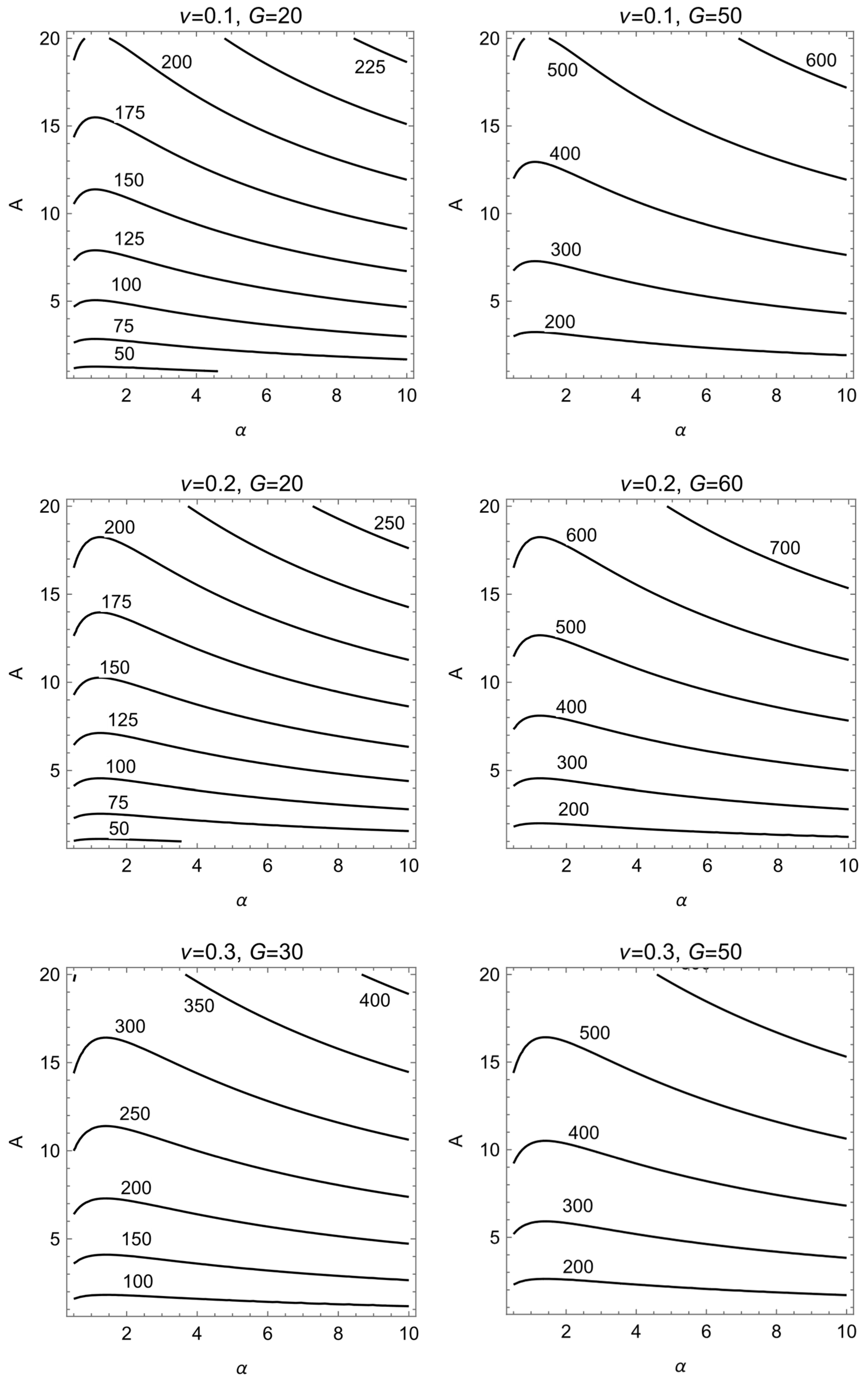
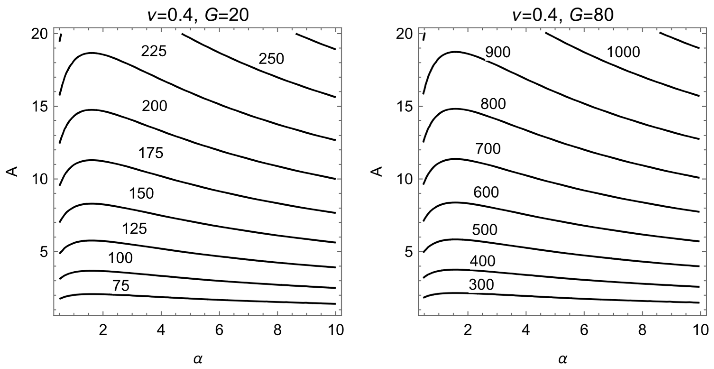
Figure 12 presents contour nomograms that show the values of the spring constant $K_x$ [MN/m] for rectangular footings with respect to foundation area A [m²] and value $\alpha ={\displaystyle \frac{a}{b}}$ [-] for different values of the shear modulus of soil G [MPa] and Poisson’s ratio ν.

Figure 13 presents contour nomograms that show the values of the spring constant $K_x$ [MN/m] for rectangular footings with respect to the shear modulus of soil G [MPa] and Poisson’s ratio $\nu$ [-] for different values of the foundation area $A$ [m²] and value $\alpha ={\displaystyle \frac{a}{b}}$ [-].

4. Discussion

The values of the spring coefficient ${\beta }_x$, which were calculated from the relationship derived in the paper (Formula (9)) for $\nu =0.3,$ are analogous to the values given in the literature, among others in papers [10,11,13,14,16], as can be seen in Figure 4. This proves that the relationships for this spring coefficient were derived correctly.

Figure 5 and Table 1 and Table 2 present the influence of different values of Poisson’s ratio ν on the ${\beta }_x$ coefficient. When comparing the obtained values of the spring coefficient ${\beta }_x$ with the values of the spring coefficient ${\beta }_x$ calculated at a constant value of ν = 0.3 (see Table 1 and Table 2), it can be seen that the differences in the obtained results are greater for a Poisson’s ratio ν < 0.3. Moreover, it can be seen that this difference increases for an increasing value of the ratio of the sides of the rectangular footing $\alpha ={\displaystyle \frac{a}{b}}$. It is the largest (of around 11.5%) for $\alpha =10$. For a Poisson’s ratio $\nu >0.3,$ the differences in the obtained results are smaller; however, for the ratio of the sides of the footing $\alpha ={\displaystyle \frac{a}{b}}=10,$ the difference is still large, i.e., about 7.8%.

It can also be noticed that for the Poisson’s ratio $\nu <0.3$, the values of the spring coefficient ${\beta }_x$ obtained from the relationship derived in this paper (Formula (9)) are higher than the values of the spring coefficient ${\beta }_x$ given in the literature (in, among others, papers [10,11,13,14,16]), i.e., calculated at a constant value of $\nu =0.3$ (compare Figure 5 and Table 1). In turn, for the Poisson’s ratio $\nu >0.3$, the values of the spring coefficient ${\beta }_x$ were lower than the values of the spring coefficient ${\beta }_x$ given in the above-mentioned literature (compare Figure 5 and Table 1). It was only for a Poisson’s ratio close to 0.5 and the ratio of the footing approaching $\alpha ={\displaystyle \frac{a}{b}}=0.5$ that the value of ${\beta }_x,$ obtained from the relationship derived in the paper (Formula (9)), was slightly (0.9%) higher than the one obtained from the calculations for a constant value of $\nu =0.3$(compare Figure 5 and Table 1).

The tendency for the initial decrease and then increase in the dimensionless spring coefficients with the change in the α coefficient, i.e., the ratio of the sides of a rectangular foundation, results from the complex interaction of several factors related to the distribution of displacements and stresses in the soil and the geometry of the foundation. Foundations closer to a square shape show larger displacements because the soil resistance is then the least effective. This occurs when the soil has difficulty generating lateral resistance across the entire width. Therefore, the value of the spring coefficient decreases. With the increase in the α coefficient, more soil begins to counteract the movement (the soil offers strong resistance) and the displacement decreases, and thus the value of the spring coefficient increases.

Based on the values of the elasticity coefficient ${\beta }_x$ obtained from numerical calculations (see Table 3 and Table 4), it can be observed that for small ratios $\alpha ={\displaystyle \frac{a}{b}}$ and Poisson’s ratio values in the range $\nu =0.1–0.3$, the agreement was obtained at the level of 3–10% with respect to the ${\beta }_x$ values obtained from analytical formulas. However, for larger values of Poisson’s ratio $\nu =0.4–0.5$, the agreement is at the level of 10–20%. With increasing ratio ${\displaystyle \frac{a}{b}}$ and Poisson’s ratio $\nu =0.5$, the difference between the results obtained from numerical and analytical calculations increases to about 28%.

Figure 8, Figure 9 and Figure 10 show the three-dimensional dependence of the spring constant $K_x$ for different values of soil parameters (the shear modulus of soil G and Poisson’s ratio of soil ν) and foundation geometry (foundation area A and the ratio of length and width of a rectangular footing $\alpha ={\displaystyle \frac{a}{b}}$). Based on Figure 8, it can be observed that the spring constant $K_x$ increases with the increasing values of the soil’s shear modulus G and the foundation area A while keeping Poisson’s ratio and the coefficient α constant. Based on Figure 9, it can be observed that the spring constant $K_x$ increases with increasing values of the coefficient α and the foundation area A while keeping the soil’s shear modulus G and Poisson’s ratio constant ν. Furthermore, the influence of the foundation area A is significantly greater than the influence of the coefficient α. Whereas based on Figure 10, it can be observed that the spring constant $K_x$ increases with increasing values of the soil’s shear modulus G and Poisson’s ratio ν while keeping the coefficient α and the foundation area A constant. Furthermore, the influence of the soil’s shear modulus G is significantly greater than the influence of Poisson’s ratio ν.

The study also furnishes valuable nomograms (presented in Figure 11, Figure 12 and Figure 13) that facilitate the direct reading of the spring constant $K_x$. These nomograms utilize common soil parameters, namely the shear modulus G and Poisson’s ratio ν, along with foundation characteristics such as area A and the aspect ratio $\alpha ={\displaystyle \frac{a}{b}}$ for rectangular foundations. As such, they can serve as a useful resource for engineers seeking rapid preliminary estimations of $K_x$ in their analyses.

The values of the spring constant $K_x$ can be calculated directly from the derived Formulas (8) and (9), or can be easily read from the nomograms (Figure 11) determined in the previous chapter. For example, for the surface area of a rectangular foundation $A=5{\mathrm{m}}^2$, the side ratio $\alpha ={\displaystyle \frac{a}{b}}=5,$ and soil parameters $\nu =0.1$ and $G=80\mathrm{M}\mathrm{N}/{\mathrm{m}}^2$, the value of the spring constant calculated from Formulas (8) and (9) is $K_x=453.018\mathrm{M}\mathrm{N}/\mathrm{m}$. In turn, the value of the spring constant calculated for the coefficient ${\beta }_x,$ given in paper [10,11,13,14,16] (i.e., at a constant value of $\nu =0.3$), is $K_x=411.085\mathrm{M}\mathrm{N}/\mathrm{m}$. Therefore, the error resulting from the application of the solution given in [10,11,13,14,16] in relation to the formulas given in this paper is (453.018 − 411.085)/411.085 = 10.20%. In turn, with similar parameters as given above, but for the side ratio $\alpha ={\displaystyle \frac{a}{b}}=10$, the value of the spring constant $K_x$ was, in the first case—$K_x=517.834\mathrm{M}\mathrm{N}/\mathrm{m}$, and in the second case—$K_x=464.348\mathrm{M}\mathrm{N}/\mathrm{m}$. Therefore, the error was already 11.52%.

In another example, for the surface area of a rectangular foundation $A=5{\mathrm{m}}^2$, the side ratio $\alpha ={\displaystyle \frac{a}{b}}=5$, and soil parameters $\nu =0.5$ and $G=20\mathrm{M}\mathrm{N}/{\mathrm{m}}^2$, the value of the spring constant calculated from Formulas (8) and (9) is $K_x=130.940\mathrm{M}\mathrm{N}/\mathrm{m}$. In turn, the value of the spring constant calculated for the spring coefficient ${\beta }_x$ given in papers [10,11,13,14,16] (i.e., for a constant value of $\nu =0.3$) is equal to $K_x=140.142\mathrm{M}\mathrm{N}/\mathrm{m}$. Therefore, the error resulting from the application of the solution given in papers [10,11,13,14,16] is equal to (130.940 − 140.142)/140.142 = −6.57%. However, with similar parameters as given above, but for the side ratio $\alpha =10,$ the value of the spring constant $K_x$ will be in the first case $K_x=145.91\mathrm{M}\mathrm{N}/\mathrm{m}$ and in the second case $K_x=158.30\mathrm{M}\mathrm{N}/\mathrm{m}$. Therefore, the error amounts to −7.83%.

The stiffness of the subsoil in the horizontal direction has a significant impact on the horizontal displacements of the entire structure or its elements, especially in the case of structures founded on flexible soils such as soft clays or peats. With the increase in the stiffness of the subsoil, the structure encounters greater resistance from the ground during horizontal displacements, which results in smaller lateral displacements. In turn, reduced stiffness of the subsoil facilitates horizontal displacements of the structure, which can lead to greater deformations and sometimes to changes in internal forces. As a consequence, this can worsen resistance to loads, e.g., seismic or wind loads. Larger structural displacements may also lead to cracking of the concrete, which may require, for example, the use of greater reinforcement or a change in the foundation system. Therefore, underestimating or overestimating the stiffness in the horizontal direction can result in less effective design in terms of safety, use, and also the economics of the structure.

In paper [10], it was found that the Poisson’s ratio ranges from about 0.25 to 0.35 for non-cohesive soils and from about 0.35 to 0.45 for cohesive soils. Lambe and Whitman, in paper [11], also state that the Poisson’s ratio can usually be assumed, with sufficient accuracy, to be equal to 0.35 for soils with low moisture content, and 0.5 for wet soils. Based on the numerical analyses carried out in this paper and by taking into account the range of the Poisson’s ratio values that may occur in real engineering cases, it should be stated that more accurate results can be obtained when using the formulas or nomograms derived here than in the case of using the nomograms previously accepted and given in the literature—in, among others, papers [10,11,13,14,16].

It should be noted that the proposed simplified approach in the calculations of structures founded on the ground, which involves adopting the spring constants ${K_x,K}_z,\mathrm{a}\mathrm{n}\mathrm{d}{K}_{\mathsf{\varphi }},$ requires an accurate determination of the geotechnical constants that appear in these formulas, i.e., the shear modulus of soil G and the Poisson’s ratio of soil $\nu$. This may constitute a certain disadvantage of the proposed method. Another limitation of the proposed method is not considering the plastic deformation that soil might undergo under extremely high loads, at which point it starts to behave like a fluid. This model also neglects the effect of foundation embedment in the soil on the spring constant. This last issue could serve as a direction for future research to be presented in a separate article.

5. Conclusions

In this paper, the formula for spring constant $K_x$ and spring coefficient ${\beta }_x$ were derived, thereby demonstrating that the spring coefficient ${\beta }_x$ depends on Poisson’s ratio ν. It was also shown that the graph presenting the dependence between the spring coefficient ${\beta }_x$ and the length–width ratio of a rectangular footing, i.e., $\alpha ={\displaystyle \frac{a}{b}}$, which was presented, among others, in papers [10,11,13,14,16], was plotted for a constant value of the Poisson’s ratio $\nu =0.3$ (see Figure 3 and Figure 4). It was shown that taking into account the Poisson’s ratio ν of a given soil significantly affects the value of the spring coefficient ${\beta }_x$, and thus affects the value of the spring constant $K_x$. The differences between the ${\beta }_x$ and $K_x$ values obtained from the calculations based on the formulas derived in this paper and from the calculations based on the formulas and nomogram for the spring coefficient ${\beta }_x$ given in, among others, papers [10,11,13,14,16] (i.e., ${\beta }_x$ calculated for the constant value $\nu =0.3$) reached 8–11%. These differences were obtained by assuming the Poisson’s ratio $\nu =0.5$ and $\nu =0.1$, and the coefficient $\alpha =10,$ for the calculations.

This paper also provides useful nomograms (see Figure 11, Figure 12 and Figure 13), which, with known soil parameters (the shear modulus of soil G and Poisson’s ratio of soil $\nu$) and foundation geometry (foundation area A and the ratio of length and width of a rectangular footing $\alpha ={\displaystyle \frac{a}{b}}$) can be used to easily read the value of the spring constant $K_x$. These nomograms can, therefore, be useful in engineering calculations for quick and preliminary estimation values of spring constant $K_x$.

Based on the results of the numerical Finite Element Method (FEM) calculations (see Table 3 and Table 4), it can be assumed that the proposed simplified approach to determining the spring coefficient yields good results (agreement at the level of 3–10% for small ratio $\alpha ={\displaystyle \frac{a}{b}}$ and Poisson’s ratio values in the range of $\nu =0.1–0.3$, and agreement of 10–28% for higher values of the analyzed parameters) in relation to the complex, three-dimensional, numerical FEM model.

The presented method in the article, the simplified method of modeling the interaction of the structure with the soil, due to its computational efficiency, can be used in preliminary engineering calculations or for the verification of complex numerical models. It should be borne in mind that the analytical methods are desirable for the correct verification of the currently used numerical methods.

The horizontal stiffness of the subsoil has a crucial impact on structural displacements, especially on flexible soils—greater stiffness limits movement, while lower stiffness increases it, potentially negatively affecting resistance and leading to damage. Incorrect estimation of this stiffness results in a less effective design in terms of safety, usability, and economics.