A Shadow Detection Method Combining Topography and Spectra for Remote Sensing Images in Mountainous Environments

Abstract

Shadow in remote sensing images can obscure important details of land features, making shadow detection crucial for enhancing the accuracy of subsequent analyses and applications. Current shadow detection methods primarily rely on the spectral information of images, which can often result in shadow misdetection due to the phenomenon of spectral confusion of different objects. To mitigate this issue, we propose a method that combines topography and spectra (CTS). Firstly, we introduce a new DEM-based shadow coarse detection method to obtain the DEM rough shadow mask, which uses a relationship between the magnitude of terrain height angle and solar elevation angle to determine shadow properties. Then, we use the MC3 (modified C3 component) index-based shadow fine detection method to obtain an MC3 mean map, which includes image enhancement with a stretching process and multi-scale superpixel segmentation. We then derive the Shadow pixel Proportion Map (SPM) by counting the DEM rough shadow mask in terms of superpixels. The Joint Shadow probability Map (JSM) is obtained by combining the SPM and the MC3 mean map with specific weights. Finally, a multi-level Otsu threshold method is applied to the JSM to generate the shadow mask. We compare the proposed CTS method against several state-of-the-art algorithms through both qualitative assessments and quantitative metrics. The results show that the CTS method demonstrates superior accuracy and consistency in detecting true shadows, achieving an average overall accuracy of 95.81% on mountainous remote sensing images.

1. Introduction

With the successive launches of high-resolution remote sensing satellites such as Jilin-1, WorldView-2, GeoEye-1, WorldView-3, GF-6, GF-7, etc., the spatial resolution of satellite remote sensing images has been continuously upgraded, which presents richer information and clearer details of land features. Shadow is a common phenomenon in remote sensing images, which is caused by direct sunlight being obscured by objects such as clouds and ground bumps. Shadows obscure critical land features, reducing image quality and readability [1]. In order to fully utilize the information provided by shadows [2,3,4,5] and eliminate the influence of shadows on the subsequent processing and application of remote sensing images, it is necessary to perform shadow detection.

Current shadow detection methods can be broadly categorized into three types: model-based methods, attribute-based methods, and deep learning-based methods.

Model-based shadow detection methods can be divided into two categories based on the data used: image model-based and elevation data-based. Image model-based methods extract information from the image itself to compute the parameters of the model [6,7,8], and then a multi-step shadow detection procedure based on the proposed model can be designed. However, when the image conditions do not satisfy the hypothesized situation, the established model may be invalid. Elevation data-based methods construct a three-dimensional light source irradiation model on the basis of elevation data to predict possible shadow areas in the image [9,10]. This approach typically requires a priori scene information such as sensor positions, camera imaging parameters, light source direction, and object geometry, which is represented by the Digital Elevation Model (DEM). Wang et al. [11] combined DEM and Sun position to detect shadows in Very High Resolution (VHR) remote sensing orthophotos and refined the coarse shadow mask generated by the high-resolution DEM with morphological operations to obtain a fine shadow mask, which is suitable for shadow detection in complex urban environments. However, the results are dependent on the accuracy of DEM and the selected parameters. While model-based shadow detection methods effectively distinguish shadows from water bodies, their performance depends heavily on the accuracy of input parameters and elevation data utilization.

Attribute-based shadow detection methods extract shadows by analyzing the differences in the spectral, texture, contextual information, geometry, and other attributes between the shadowed regions and non-shadowed regions in images [12,13,14,15,16,17,18,19]. Compared to model-based methods, these methods usually do not require the inclusion of a priori information and only perform shadow detection based on existing image features. Because the image features are relatively easy to obtain, attribute-based methods have a wide range of applications. Silva et al. [20] proposed a shadow detection method based on the Logarithmic Spectral Ratio Index (LSRI) by considering the data compression characteristics of logarithmic operations. Liu et al. [21] proposed the Normalized Color Difference Index (NCDI) and Color Purity Index (CPI) by analyzing the different reflectance characteristics of shadows, vegetation, and water in visible and near-infrared wavelengths, which can effectively enhance shadows by suppressing the characteristics of dark features. Wang et al. [22] combined the Simple Linear Iterative Clustering (SLIC) method and LSRI to detect three types of shadows in mountainous areas caused by terrain, clouds, and buildings, which achieves good detection results. However, if there are dark water bodies and vegetation in the image, the method still cannot avoid the problem of shadow misdetection. Overall, attribute-based shadow detection methods can accurately locate the boundary and outline of shadow regions by analyzing the detailed attributes of the image using color, texture, and gradient information. However, it is difficult to select highly universal optimal features, and inappropriate feature selection may lead to shadow misdetection or omission. Moreover, they are unable to accurately differentiate between water bodies, low-reflectance objects, and shadows due to the problem of spectral similarity.

Deep learning-based shadow detection methods recognize shadow regions by learning shadow patterns in images [23,24,25,26,27,28,29,30,31,32,33,34,35]. Commonly used neural network structures for shadow detection include Convolutional Neural Networks (CNNs), Generative Adversarial Networks (GANs), and networks based on attention mechanisms. Instead of manually designing shadow features as in traditional methods, deep learning methods enable the discovery of high semantic features through complex and dense network connections. Luo et al. [36] proposed the first Aerial Imagery dataset for Shadow Detection (AISD) and, accordingly, proposed a Deeply Supervised convolutional neural network for Shadow Detection (DSSDNet), which solves the problem of insufficient shadow feature extraction by adopting the encoder-decoder residual structure. Zhang et al. [37] proposed a Multi-Resolution Parallel Fusion Attention Network (MRPFANet), which improves the ability to extract spatial information and shadow features from images by incorporating a cross-space attention module and a channel attention module. In recent research, deep models have been used to segment shadows in videos [38], and deep models that use the Transformer architecture as a backbone network [39,40] are also being used more often for shadow detection in images. However, although deep learning methods show high robustness in specific scenes, they require massive amounts of training data as input, and the cost of manually labeling is too high. Additionally, the extraction of deep features is not fully sufficient, as high-level features still tend to mix with low-level features, making it challenging to distinguish independent shadow features.

In this paper, we propose a shadow detection method that combines topography and spectra (CTS). Based on the spectral attributes used to detect shadows, we exploit the terrain information of the elevation data to avoid the misdetection caused by spectral similarity. In cases where the image contains large areas of dark objects mixed with shadows, such as vegetation and water bodies, CTS can accurately identify shadows, leading to a significant improvement in detection performance compared to existing methods.

The rest of this paper is organized as follows. In Section 2, the relevant theories and the proposed framework are described in detail. Section 3 presents the experimental results with a comparison. In Section 4, the experimental parameters are analyzed. The conclusions are provided in Section 5.

2. Materials and Methods

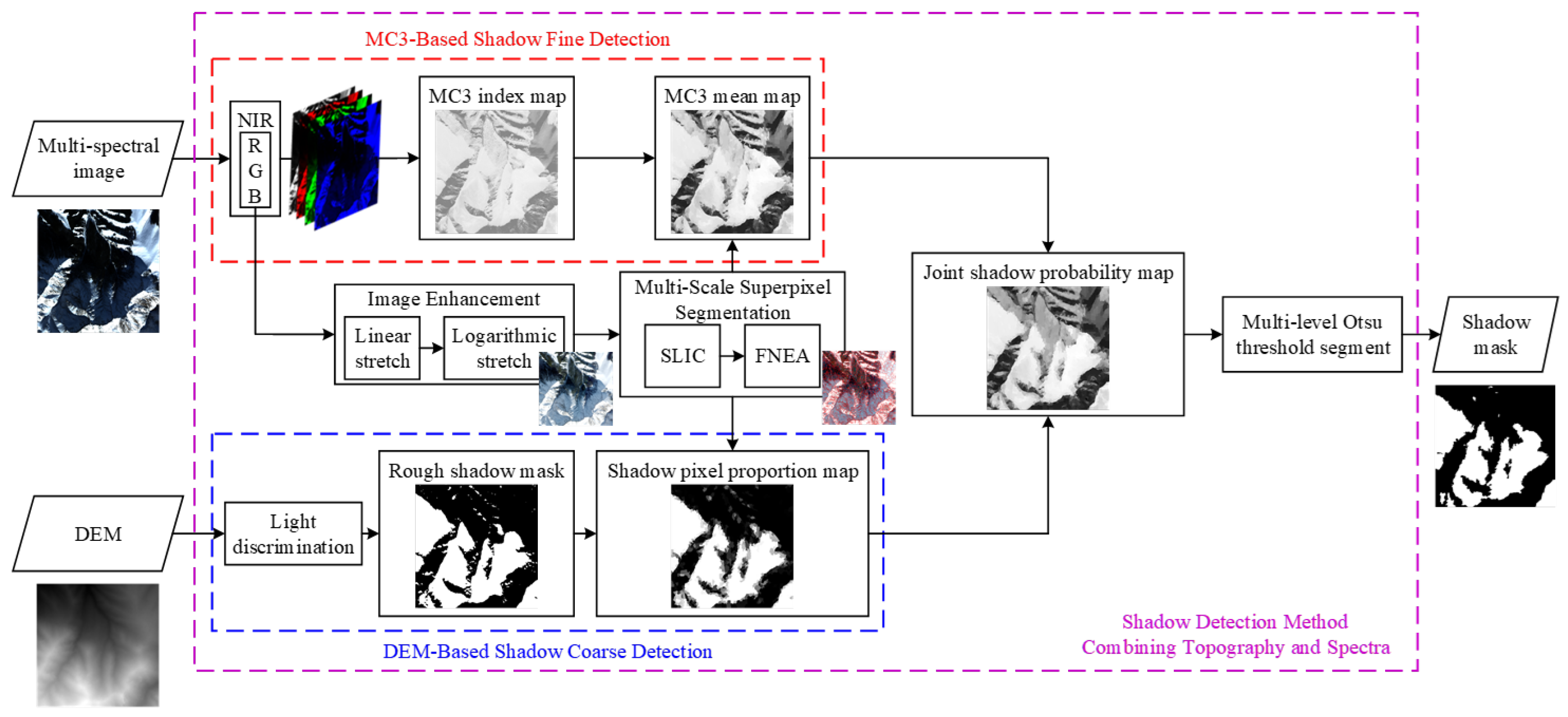
The proposed CTS method consists of two parts: coarse shadow detection based on DEM and fine shadow detection based on the MC3 index. Firstly, we perform image enhancement [41] with linear and logarithmic stretching on the ortho-corrected RGB image to extend the low gray range of the image to better separate the shadow from the background. Then, the Fractal Net Evolution Approach (FNEA) based on SLIC is performed on the enhanced image to generate multi-scale superpixels for the subsequent shadow detection. DEM-based coarse shadow detection uses DEM data as input to obtain a rough shadow mask; MC3-based fine shadow detection utilizes the RGBNIR four-band pixel values of the image for the calculation of the MC3 shadow index. Subsequently, We derive the Shadow-pixel Proportion Map (SPM) and the MC3 mean map based on superpixels. These two maps are then fused with specific weights to generate the Joint Shadow probability Map (JSM), which indicates the likelihood of each superpixel belonging to the shadow. Finally, we apply a multi-level Otsu threshold to the JSM to generate the final shadow mask. Figure 1 illustrates the CTS processing flowchart.

2.1. Image Enhancement

The pixel values of remote sensing images are generally stored in 10 or 11 bits. In order to facilitate subsequent superpixel segmentation, the images are converted to 8 bits by 2% linear stretching. Then, the logarithmic stretching is used to expand the darker part of the image by utilizing its property of steep change in a low-value range so that the difference between real shadows and non-shadowed dark regions in the enhanced image is more obvious. The logarithmic function is defined as follows:

$$g(x,y)=c·{log}_{(1+v)}(1+v·f(x,y))$$

(1)

where c is a constant coefficient, usually set to 1. The larger v indicates the higher degree of logarithmic stretching, and the pixel value of the original image at $(x,y)$ is $f(x,y)\in [0,1]$. Figure 2 illustrates the logarithmic curves corresponding to different values of v.

Figure 3 illustrates the images and their corresponding histograms after different degrees of logarithmic stretching. The values of dark vegetation and shadow in the image before stretching are similar, which cannot be effectively distinguished by the naked eye, while after logarithmic stretching, the dark vegetation and shadow are easier to distinguish visually. It can be seen that logarithmic stretching can show more details of the low gray part of the image and highlight the shadow in the image, which is important for the subsequent superpixel segmentation and shadow detection.

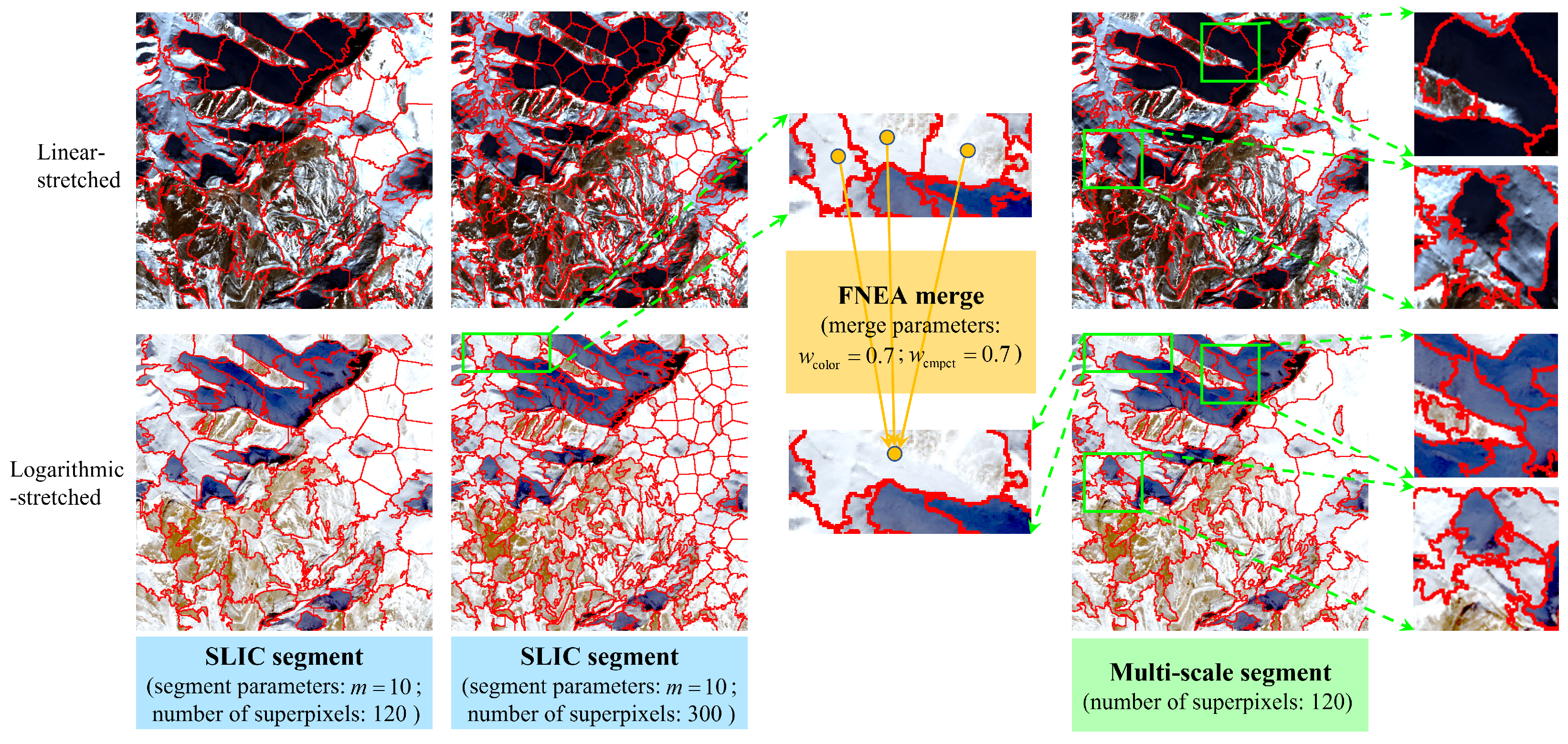
2.2. Multi-Scale Superpixel Segmentation

Applying the shadow index calculation to the image produces the corresponding shadow index map. However, directly thresholding this index map to extract shadows can result in numerous dense separation points and false alarms. In order to overcome the effect of noise and to protect the integrity of shadow edges, ensuring the continuity and integrity of shadow superpixel, superpixel segmentation can be performed on the image. The superpixel segmentation of images may have the problem of over-segmentation and under-segmentation, which is difficult to balance. In the shadow detection task, under-segmentation may cause the shadows and non-shadows to be mixed in the same object, and the over-segmentation will unnecessarily increase computation costs. Therefore, we adopt a multi-scale segmentation method. We first use the SLIC [42] method to generate an initial large number of superpixels. Then, we use FNEA [43] to merge spectrally similar and spatially close SLIC superpixels to form a multi-scale segmentation result. FNEA is a bottom-up superpixel segmentation method that views the image as a four-neighborhood Region Adjacency Graph (RAG) based on the idea of graph theory. It combines the spectral features and shape features of multiple bands to describe the node characteristics. The neighboring nodes are then merged according to the merging cost in a Nearest Neighbor Graph (NNG). We use the superpixels obtained by over-segmentation of SLIC as the starting nodes for merging by FNEA. This way, we can avoid the problem of mixing shadows and non-shadows to the greatest extent while having a suitable number of superpixels.

Figure 4 illustrates the multi-scale segmentation method we use and its segmentation results on the two stretch-processed images. We set the number of over-segmented superpixels $n_o$ as the iterative stopping control quantity for SLIC and the number of merged superpixels $n_m$ to control the iteration of FNEA. We define the average area of merged superpixels $a_m$, then $n_m=M\times N/a_m$, where M and N are the number of rows and columns of the image.

The shadow and the background in the linear-stretched image are more likely to be mixed in the same object, and the superpixel contour cannot closely adhere to the real shadow edge, while the superpixels in the logarithmic-stretched image are able to segment shadows more accurately. Compared with single-scale, the multi-scale segmentation results are more hierarchical, with more superpixels and smaller sizes in the dark region containing shadows and fewer superpixels and larger sizes in the non-shadowed background. All in all, multi-scale superpixel segmentation of the logarithmic-stretched image can separate the shadow and background more clearly in the form of image objects. It can ensure the continuity and integrity of shadows, which creates a good condition for the subsequent shadow processing.

2.3. DEM-Based Shadow Coarse Detection Method

The DEM-based shadow coarse detection method is used to determine the presence or absence of light for each point in the DEM raster, which involves calculating the maximum of the terrain height angles formed by the points within the shade analysis radius toward the Sun for each point. If the maximum terrain height angle is less than the solar elevation angle at that moment, then the point is in light; otherwise, there is no light.

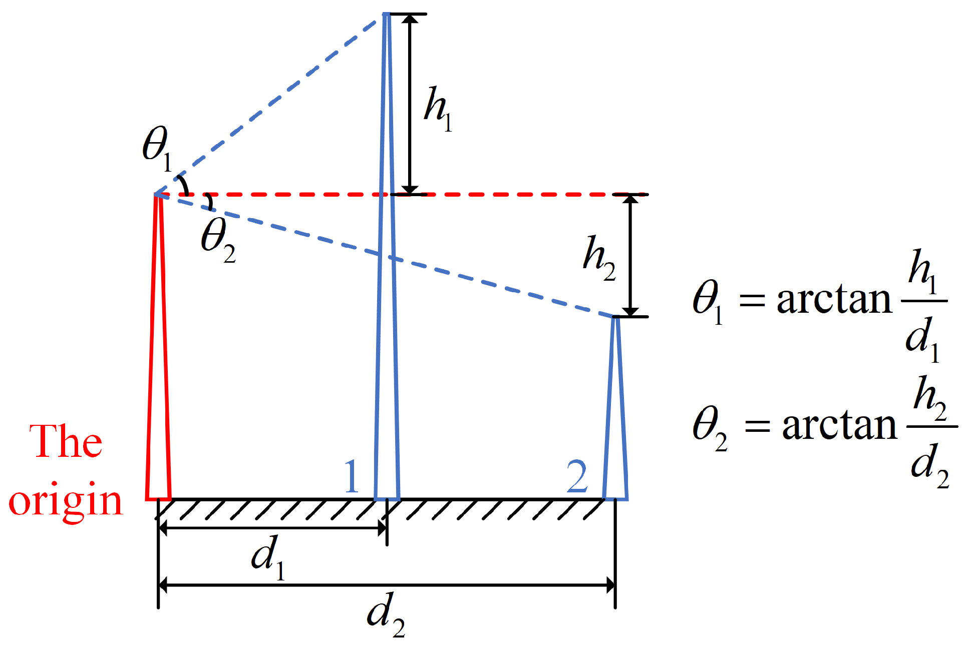
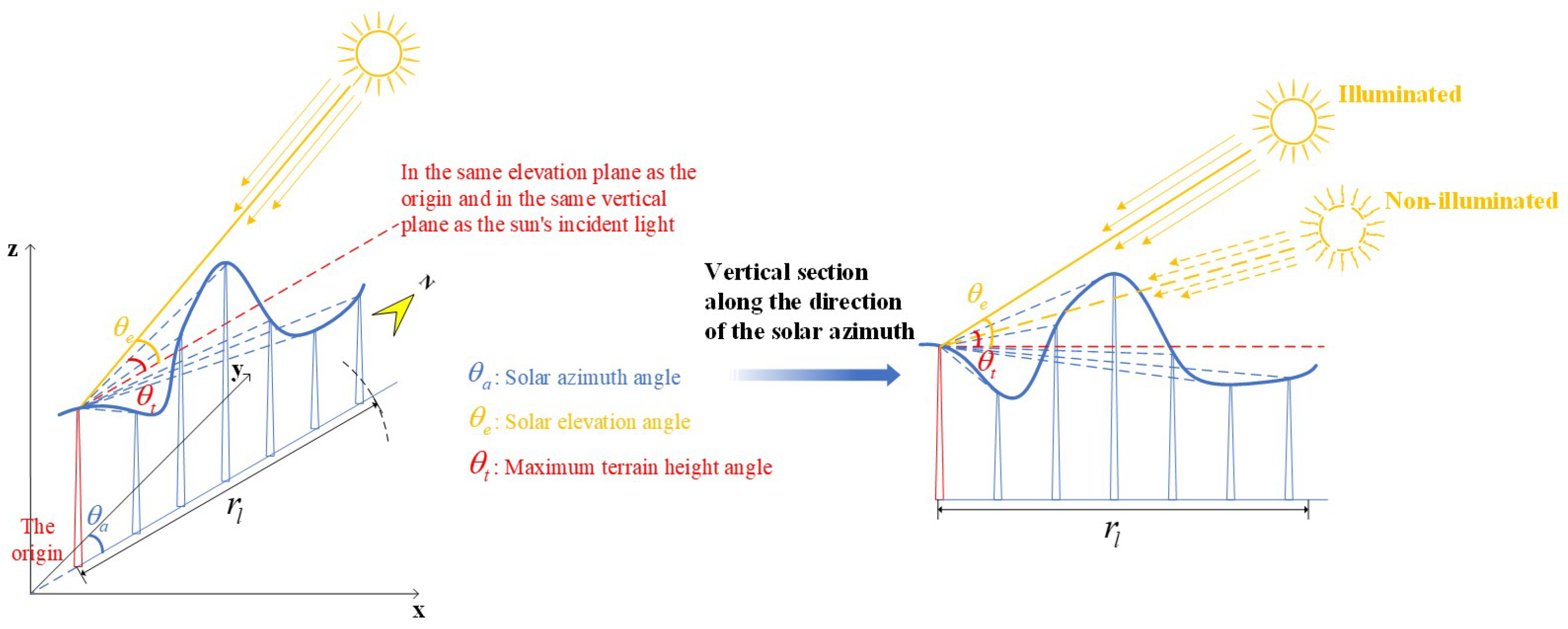
2.3.1. Terrain Height Angle

The terrain height angle between two points is caused by the elevation difference between them. As shown in Figure 5, the terrain height angles between points 1, 2, and the origin are ${\theta }_1$ and ${\theta }_2$, respectively. We set the elevation difference to be positive when the elevation of other points is greater than that of the origin; it is negative otherwise. As shown in Figure 5, the elevation difference is $h_1>0$ and $h_2<0$, and accordingly, the terrain height angle is ${\theta }_1>0$ and ${\theta }_2<0$. If the elevations of the two points are equal, the terrain height angle is $0°$; if the elevation difference tends to infinity, such as the cliffs in real life, the terrain height angle is $\pm 90°$.

2.3.2. Shade Analysis Radius

When calculating the maximum terrain height angle of the origin in the direction of the solar azimuth, it is necessary to determine what points on the ray are to be counted. Each of these terrain height angles, formed by the potential points and the origin, may be greater than the origin’s solar elevation angle at that time. We can set a shade analysis radius and then locate the points centered on the origin in the ray toward the Sun within the radius. The presence or absence of light at the origin can be determined by simply calculating these points. Figure 6 illustrates the diagram for determining whether the origin is illuminated or not.

The significance of the shade analysis radius is that for the origin, as long as the points on the line within the radius do not block the light, then there will be no point outside the radius that can block the light; if there is a blocking point within the radius, that is, the terrain height angle between the point and the origin is greater than the solar elevation angle, then the origin is in shadow. The shade analysis radius is different for different moments and different points.

Calculating the shade analysis radius is a two-step process: firstly, calculate the global shade radius $r_g$, and then calculate the local shade radius $r_l$ within $r_g$. The global shade radius is the range covered by the highest point of the earth relative to the origin at this time. Find the highest elevation among all the points located within the range $r_g$ along the ray towards the Sun, and then calculate the range covered by this elevation relative to the origin at this time, which is the local shade radius.

In Figure 7, A is the location of the point where we want to calculate the shade analysis radius, and point B is the virtual location of the highest point in the world (Mt Everest 8848.86 m), which is determined based on the global shade radius of A. That is, the furthest point of the shade caused by B at this time is A.

We can calculate the solar elevation angle of A${\theta }_e$ according to its latitude and longitude at this time. Whether A is shaded is only related to the relationship between the terrain height angle and the solar elevation angle, while the terrain height angle is only related to the elevation difference. So, we only need to consider the difference between the elevation of the highest point $h_p$, and the elevation of A$h_i$. Therefore, the elevation of B can be set to $h_p-h_i$ and the elevation of A is zero.

Knowing the mean radius of the earth $R_e=6.371\times {10}^6$ m, the global shade radius of A$r_g$ and the dip angle of the line connecting AB with respect to the horizon at A${\theta }_{d1}$ can be obtained by making a system of equations as follows:

$$\left\{\begin{array}{c}{r}_g·tan{\theta }_e+r_g·tan{\theta }_{d1}=h_p-h_i\hfill \\ R_e·tan\left(2{\theta }_{d1}\right)=r_g\hfill \end{array}\right.$$

(2)

The global shade radius is the longest and most specific type of shade analysis radius. In practice, the local shade radius may not be equal to the global shade radius unless the sampling area is located near the highest point. The global shade radius only provides a pre-defined reference range within which to find and compute a realistic local shade radius for the point without considering a longer range.

Find the highest point C on the ray of A towards the Sun within $r_g$, the elevation of which is $h_j$, and then make the same set of equations to obtain $r_l$:

$$\left\{\begin{array}{c}{r}_l·tan{\theta }_e+r_l·tan{\theta }_{d2}=h_j-h_i\hfill \\ R_e·tan\left(2{\theta }_{d2}\right)=r_l\hfill \end{array}\right.$$

(3)

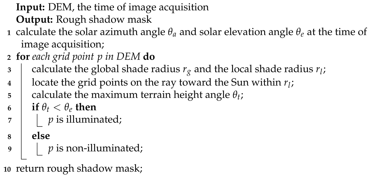
For the origin, the maximum terrain height angle formed by the points on the line within the local shade radius is calculated and compared to the solar elevation angle to find out if there is light or not. Then, a shadow mask is generated by judging the shadow attribute for each point in the DEM raster. The pseudo-code for DEM-based shadow coarse detection algorithm is shown in Algorithm 1.

Algorithm 1: DEM-based shadow coarse detection

Because the resolution of the DEM used is generally lower than that of the image, the shadow mask obtained from DEM is generally smaller than the original image. So, we extend the DEM shadow mask to the same size as the image by interpolation.

The shadow masks derived from this method are rough due to factors such as the accuracy of the DEM, the error in the calculation of the solar angles, and the ortho-correction of the image. If the shadow mask is derived using the solar elevation angle and azimuth angle at the moment the image was taken, the DEM-based method can predict the approximate location of shadows in the image, which can guide the subsequent shadow fine detection.

2.4. MC3-Based Shadow Fine Detection Method

In addition to rough detection of shadows based on external a priori knowledge, fine detection of shadow can be achieved by discriminating shadows with features extracted from the image itself, which requires the spectral features that distinguish shadows from other dark ground objects.

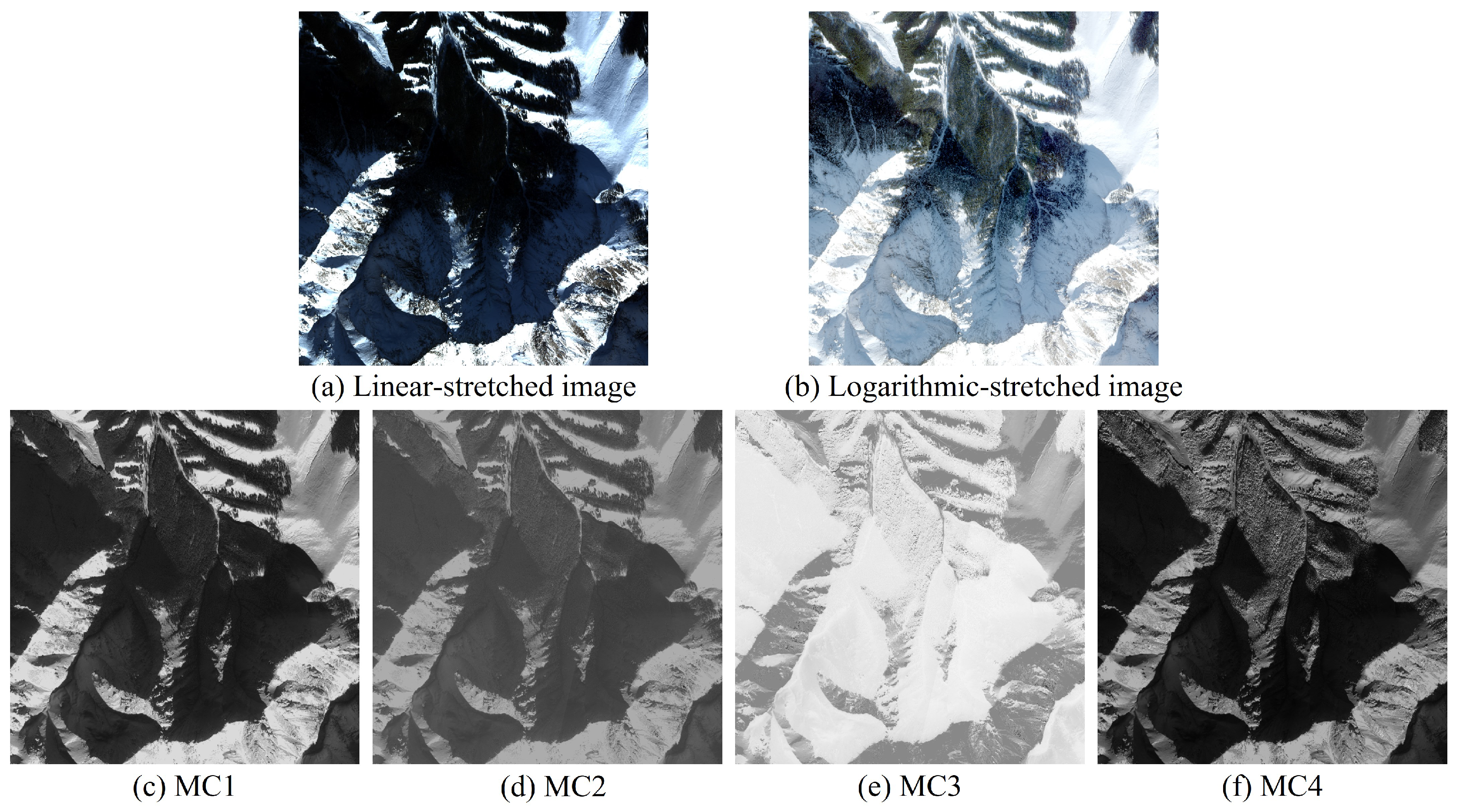
The C1C2C3 color space is a form of nonlinear transformation of the RGB color space. Besheer et al. [15] improved the C1C2C3 color space by adding near-infrared band information and proposed an MC1C2C3C4 color space with a modified C3 component (MC3):

$$\begin{array}{cc}\hfill M{C}_1& =arctan\left({\displaystyle \frac{R}{\max (G,B,NIR)}}\right)\hfill \\ \hfill M{C}_2& =arctan\left({\displaystyle \frac{G}{\max (R,B,NIR)}}\right)\hfill \\ \hfill M{C}_3& =arctan\left({\displaystyle \frac{B}{\max (R,G,NIR)}}\right)\hfill \\ \hfill M{C}_4& =arctan\left({\displaystyle \frac{NIR}{\max (R,G,B)}}\right)\hfill \end{array}$$

(4)

The MC3 component has the highest brightness in the shadow region of the image by virtue of the increased weight of the blue component in shadows and the lower shadow reflectance values in the near-infrared band. Figure 8 illustrates the four components of the MC1C2C3C4 space of an image. It can be seen that in the MC3 image, the shadow region has the highest value. The dark vegetation around the shadow has relatively low values, but the difference is not large.

Only using spectral properties to perform detection makes it especially easy to confuse shadows with dark objects, such as vegetation, water bodies, soil, etc. The image may also have uneven brightness inside the shadow due to the different reflectance of features in the shadow-covered area, which will interfere with the recognition of shadows and lead to shadow misdetection and omission. This problem can be avoided to some extent by combining the topographic factors brought by DEM.

2.5. Shadow Detection Method Combining Topography and Spectra

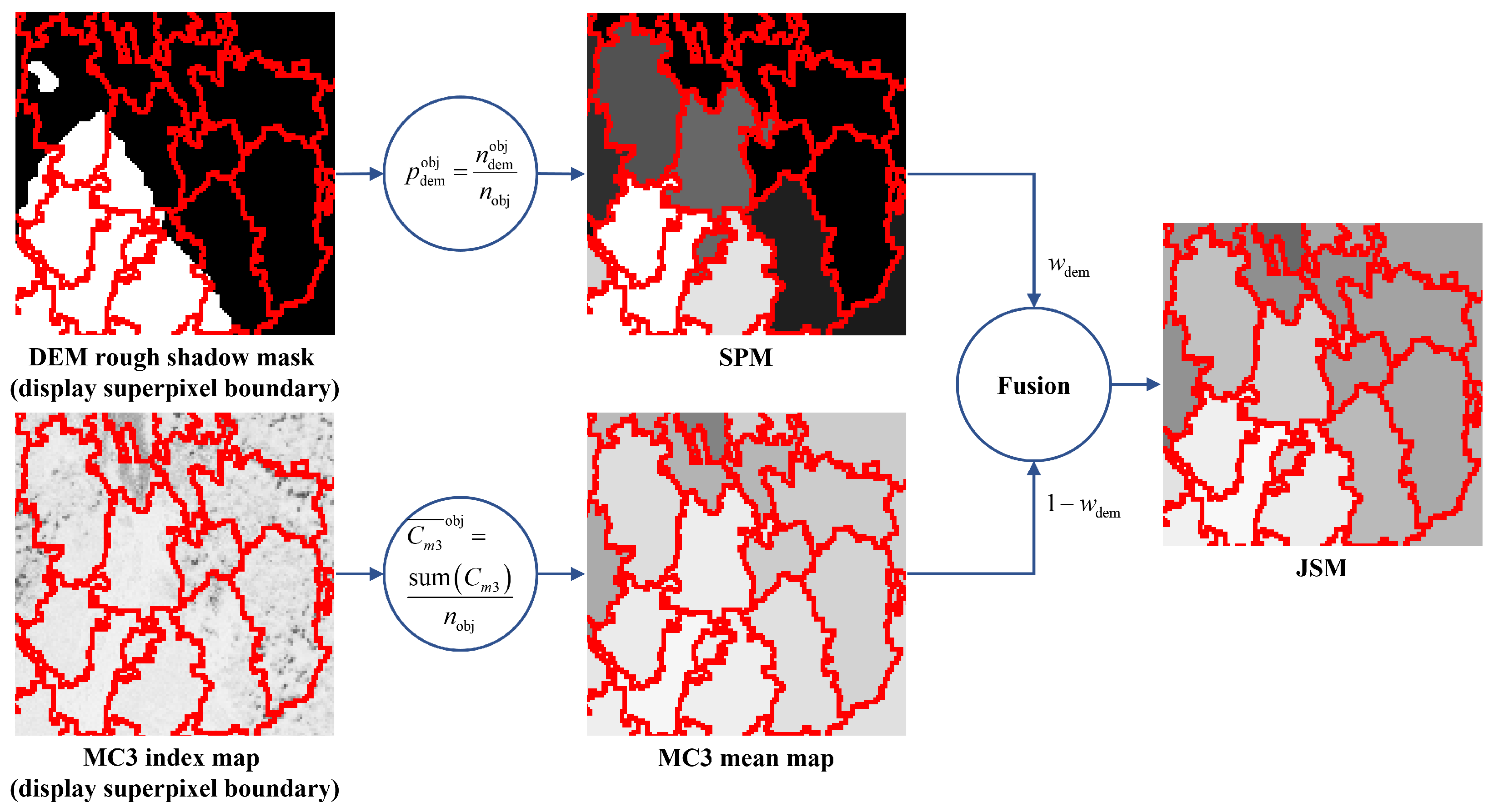
The image is divided into several homogeneous regions, i.e., image objects, after superpixel segmentation. The CTS method is performed on these homogeneous regions. The proportion of shadow pixels contained within each image object is determined by the DEM rough shadow mask as follows:

$$p_{\mathrm{dem}}^{\mathrm{obj}}={\displaystyle \frac{n_{\mathrm{dem}}^{\mathrm{obj}}}{n_{\mathrm{obj}}}}$$

(5)

where $n_{\mathrm{dem}}^{\mathrm{obj}}$ is the total number of shadow pixels in the DEM rough shadow mask contained within the object, and $n_{\mathrm{obj}}$ is the total number of pixels in the object. After calculating $p_{\mathrm{dem}}^{\mathrm{obj}}$ for all objects, the SPM can be obtained, which reflects the probability that each object is geographically in shadow.

The mean value of MC3 is calculated for each image object:

$${\overline{C_{m3}}}^{\mathrm{obj}}={\displaystyle \frac{{\sum }_{(x,y)\in \mathrm{obj}}{C}_{m3}(x,y)}{n_{\mathrm{obj}}}}$$

(6)

where $C_{m3}(x,y)$ is the pixel value of $(x,y)$ in the MC3 component. After assigning all objects their MC3 mean values, the MC3 mean map can be obtained, which reflects the probability that each object belongs to shadow on the spectra.

The probability that each image object belongs to shadow is shown as follows:

$$P_s^{\mathrm{obj}}=w_{\mathrm{dem}}·p_{\mathrm{dem}}^{\mathrm{obj}}+(1-w_{\mathrm{dem}})·{\overline{C_{m3}}}^{\mathrm{obj}}$$

(7)

where ${\overline{C_{m3}}}^{\mathrm{obj}}$ is normalized to the $[0,1]$ range, $w_{\mathrm{dem}}$ is the weight of the DEM rough shadow mask, and $(1-w_{\mathrm{dem}})$ is the weight of the MC3 mean map, which controls the degree of influence of topography and spectra on shadow detection. In that way, the topography can correct the shadow misclassification due to spectral similarity and the spectra can correct the roughness and inaccurate localization of the terrain in detecting shadows. Both of them can correct each other’s shadow misdetection and omission problems so that the shadow detection accuracy can be further improved.

Figure 9 demonstrates the process of generating the JSM. After fusing the two maps to generate the superpixel JSM of the image, the final shadow mask can be obtained by applying the multi-level Otsu threshold method to the histogram of JSM in terms of superpixels.

3. Results

In this section, we perform DEM-based, MC3-based (hereafter referred to as MC3), and CTS methods on several images to illustrate the effectiveness of our proposed algorithms. The detection results are evaluated qualitatively and quantitatively. Three conventional shadow detection algorithms, Silva’s [20], Wang’s [22], and Zhou’s [18], as well as two deep learning-based methods, Guan’s [34] and ECA [35], are used as comparisons to demonstrate the superiority of the proposed methods in accurately recognizing shadows and avoiding shadow misdetection. For the DEM-based method, we focus more on visual evaluation because it is difficult to obtain the ground truth. The experiment images are from GF07 with a resolution of 2.6 m, containing RGBNIR four bands. The DEM used has three resolutions: 5 m, 12.5 m, and 30 m.

3.1. Experimental Setting

In all algorithms, the parameters are set as follows: the Silva, Wang, and Zhou methods are reproduced according to the optimal parameters provided in their papers. The Guan and ECA methods were experimented on using the parameters of the pre-trained model provided online. For MC3, $n_o$ and $a_m$ are 3000 and 1200, respectively. The maximum threshold is determined by the histogram of superpixels with the number of thresholds $c=3$. For CTS, $n_o=3000$ and $a_m=1200$. The number of thresholds is $c=3$. The merging weight is $w_{\mathrm{dem}}=0.2$. It is a manually set parameter and an empirical value. Extensive experiments have demonstrated that setting it as 0.2 is appropriate for most mountain images. The images used by MC3 and CTS are enhanced by 2% linear stretching and logarithmic stretching with $v=100$.

3.2. Evaluation Indicators

The shadow detection results of images can be evaluated using the producer’s accuracy, user’s accuracy, committed error, omitted error, overall accuracy, and kappa coefficient from the confusion matrix [44], as summarized in

Table 1. Evaluation indicators for shadow detection.

	Producer’s Accuracy	Users’ Accuracy	Committed Error	Omitted Error	Overall Accuracy
Shadow	$P_s={\displaystyle \frac{\mathrm{TP}}{\mathrm{TP}+\mathrm{FN}}}$	$U_s={\displaystyle \frac{\mathrm{TP}}{\mathrm{TP}+\mathrm{FP}}}$	$E_c={\displaystyle \frac{\mathrm{FP}}{\mathrm{FP}+\mathrm{TN}}}$	$E_o={\displaystyle \frac{\mathrm{FN}}{\mathrm{FN}+\mathrm{TP}}}$	$\tau ={\displaystyle \frac{\mathrm{TP}+\mathrm{TN}}{\mathrm{TP}+\mathrm{TN}+\mathrm{FP}+\mathrm{FN}}}$
Non-shadow	$P_n={\displaystyle \frac{\mathrm{TN}}{\mathrm{TP}+\mathrm{TN}}}$	$U_n={\displaystyle \frac{\mathrm{TN}}{\mathrm{FN}+\mathrm{TN}}}$

.

A higher producer’s accuracy and user’s accuracy for shadows, as well as a lower omitted error, indicate the better ability of the shadow detection method to recognize shadows. A higher producer’s accuracy and user’s accuracy for non-shadows and a lower committed error indicate its better ability to distinguish non-shadows [45]. Overall accuracy refers to the ratio of the number of correctly categorized pixels to the total number of pixels in the image, with higher levels indicating a better overall capability of the shadow detection method. A higher kappa coefficient indicates the shadow mask is closer to the ground truth. Ideal shadow detection methods should usually have a higher producer’s accuracy, user’s accuracy, overall accuracy, and kappa coefficient, as well as a lower committed error and omitted error.

3.3. DEM-Based Shadow Coarse Detection

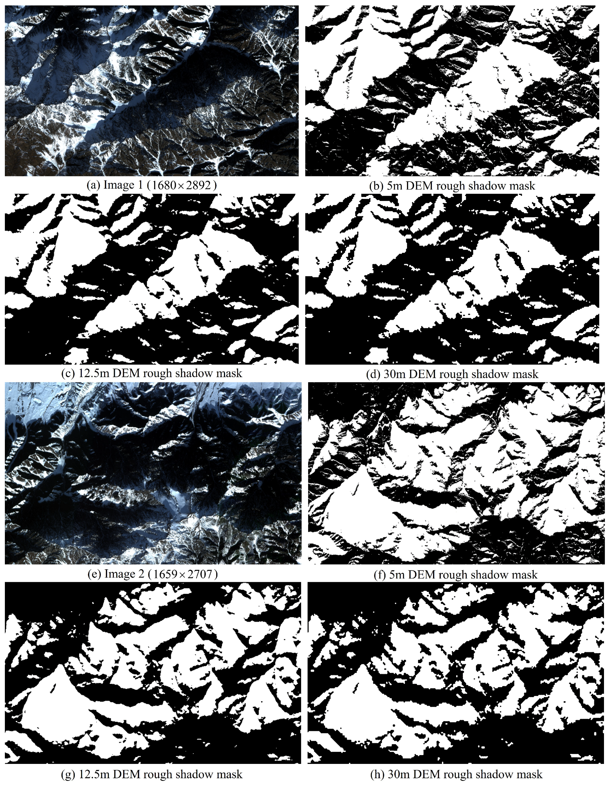
DEM-based shadow coarse detection first needs to determine the location of the quadrangle points of the coarse shadow mask on the DEM and calculate the solar azimuth and elevation angle at the moment of image acquisition. We choose Image 1 and Image 2 to perform shadow detection with a 5 m, 12.5 m, and 30 m DEM. Figure 10 illustrates the results. The white part of the shadow mask is shadow, and the black part is the background. We can see that the DEM rough shadow mask is able to recognize most of the shadows in the image. It has an effective localization on the main shadow areas. However, because the DEM is not accurate enough to reach the same resolution as the image, the rough shadow mask cannot have a close fit with the real shadow.

Because of the lower resolution, the 30 m DEM shadow mask is rougher than the 12.5 m, but overall, it does not affect the effectiveness in locating shadow areas. The 5 m DEM is generated by combining the 12.5 m DEM with forward and backward panchromatic stereo images. Its shadow mask has more refined shadow regions with more complete edges, and it fits to the original image better. However, a high-resolution DEM is difficult to obtain, and the actual cost of detecting shadows with them is high.

The rough shadow mask may have problems with shadow edges fitting inaccurately and with positional offsets. Although its direct detection of shadow cannot reach ideally high accuracy, it can be used to locate the main shadow areas to avoid the misdetection of non-shadowed dark ground objects.

3.4. MC3-Based Shadow Fine Detection

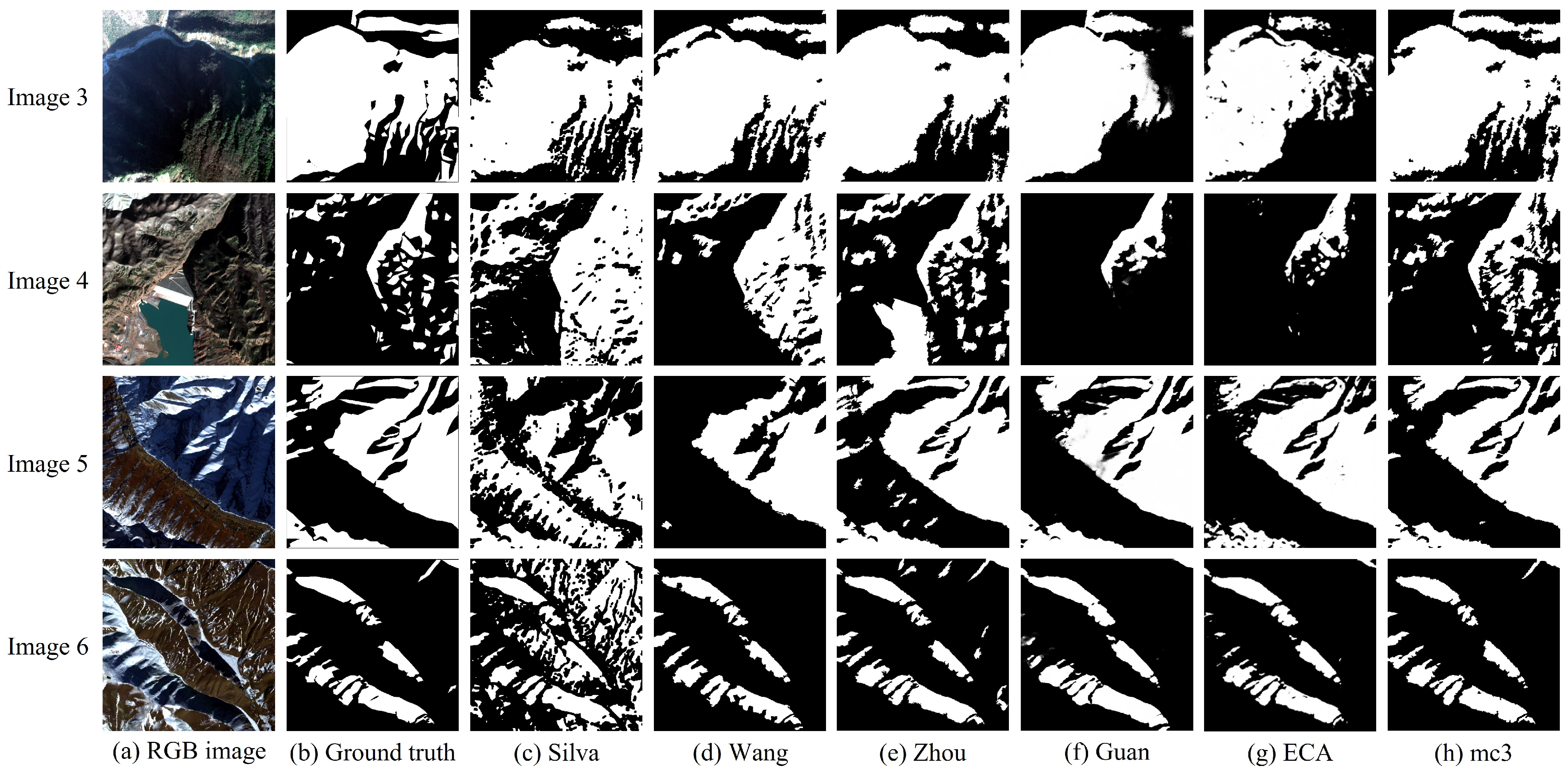
In this paper, four $512\times 512$ size images were subjected to shadow fine detection using MC3. Figure 11a presents four images of mountains with different scenes. Image 3 contains whole, large and thin, small areas of shadows, in which thin shadows are interspersed with dark vegetation. Image 4 has some fragmented shadows of mountains, which are interspersed with dark vegetation. Image 5 contains dark soil and large shadow areas. Image 6 contains regularly distributed shadows among dark soil.

The corresponding ground truth images are shown in Figure 11b. The detection results of Silva, Wang, Zhou, Guan, ECA, and our MC3 are shown in Figure 11c–h, respectively.

Table 2. Quantitative evaluation results of shadow detection.

Image	Method	${\mathit{P}}_{\mathit{s}}$ (%)	${\mathit{P}}_{\mathit{n}}$ (%)	${\mathit{U}}_{\mathit{s}}$ (%)	${\mathit{U}}_{\mathit{n}}$ (%)	${\mathit{E}}_{\mathit{c}}$ (%)	${\mathit{E}}_{\mathit{o}}$ (%)	$\mathit{\tau }$ (%)	$\mathit{kappa}$
3	Silva	81.83	91.06	94.43	73.02	8.94	18.17	85.06	0.69
	Wang	94.78	83.93	91.61	89.68	16.07	5.22	90.98	0.80
	Zhou	93.25	92.31	95.74	88.07	7.69	6.75	92.92	0.85
	Guan	79.87	93.68	95.90	71.54	6.32	20.13	84.71	0.69
	ECA	75.78	98.09	98.66	68.63	1.91	24.22	83.61	0.67
	Ours (MC3)	95.06	89.15	94.19	90.69	10.85	4.94	92.98	0.85
4	Silva	99.08	56.18	28.91	99.71	43.82	0.92	62.72	0.28
	Wang	94.50	73.63	39.19	98.67	26.37	5.50	76.81	0.43
	Zhou	89.84	81.82	47.06	97.82	18.18	10.16	83.04	0.52
	Guan	44.66	98.73	86.32	90.84	1.27	55.34	90.48	0.54
	ECA	40.14	99.39	92.23	90.23	0.61	59.86	90.36	0.51
	Ours (MC3)	91.48	89.10	60.15	98.31	10.90	8.52	89.46	0.66
5	Silva	67.70	66.47	64.48	69.60	33.53	32.30	67.05	0.34
	Wang	70.05	98.47	97.63	78.53	1.53	29.95	85.01	0.70
	Zhou	96.60	91.64	91.21	96.78	8.36	3.40	93.99	0.88
	Guan	95.32	95.07	94.56	95.77	4.93	4.68	95.19	0.90
	ECA	91.41	97.15	96.64	92.64	2.85	8.59	94.43	0.89
	Ours (MC3)	95.36	96.65	96.23	95.86	3.36	4.64	96.04	0.92
6	Silva	91.68	71.00	34.87	98.06	28.99	8.32	74	0.37
	Wang	83.90	98.32	89.45	97.30	1.68	16.10	96.24	0.84
	Zhou	96.98	97.03	84.69	99.48	2.97	3.02	97.02	0.89
	Guan	91.16	96.34	80.83	98.47	3.66	8.84	95.59	0.83
	ECA	87.76	98.31	89.78	97.94	1.69	12.24	96.78	0.87
	Ours (MC3)	92.90	98.44	90.98	98.79	1.56	7.10	97.64	0.91

Note: The values in bold indicate the best performance.

summarizes the quantitative evaluation results of the six methods.

3.5. Shadow Detection Combining Topography and Spectra

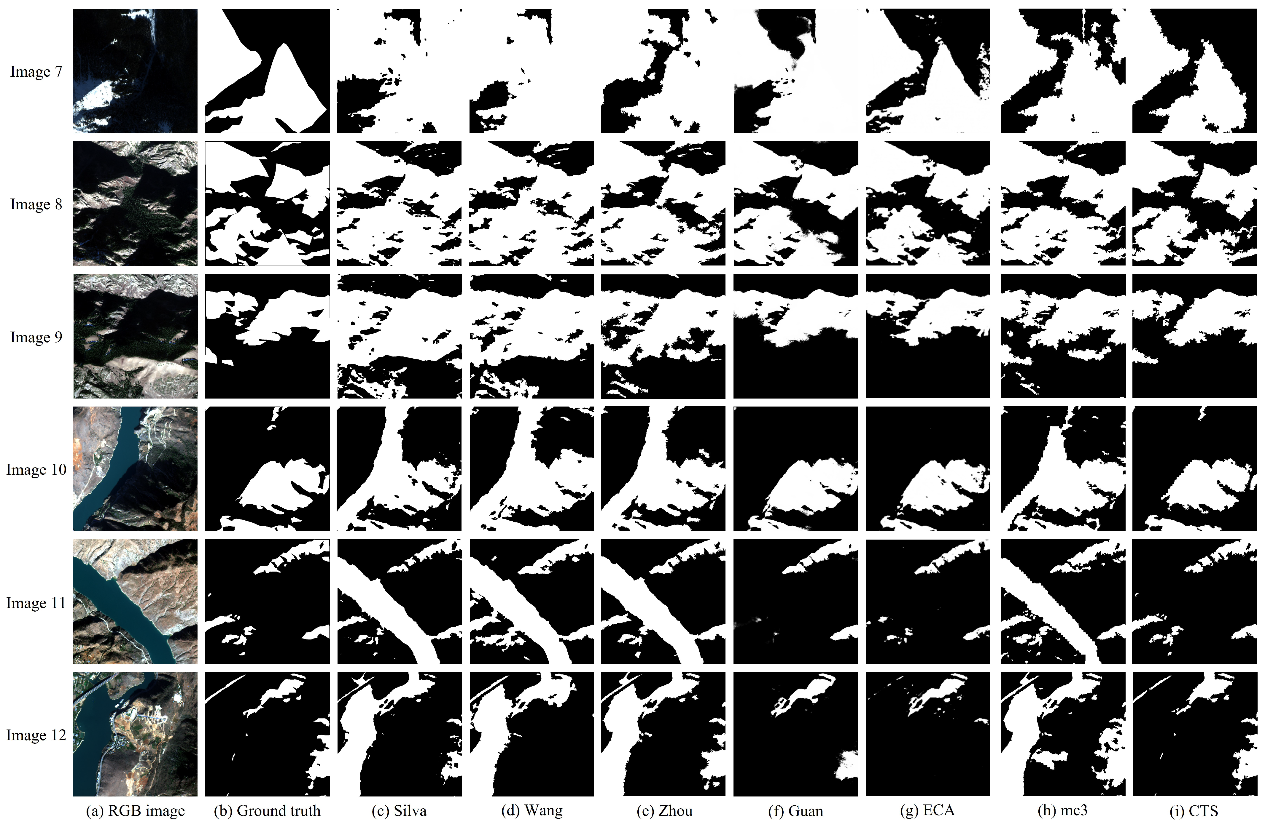
The proposed CTS method has two inputs: the image and the DEM corresponding to the image’s geographic location. We used six $512\times 512$ size mountainous images to conduct the experiments. The six images contain two types of features that easily cause shadow confusion, which are vegetation and water body.

Table 3. Information about the experimental images for CTS.

Images	Center Longitude	Center Latitude	Feature Type	Province
Image 7	87.03 E	43.45 N	vegetation	Xinjiang
Image 8	86.55 E	43.67 N
Image 9	86.50 E	43.68 N
Image 10	100.60 E	26.19 N	water body	Yunnan
Image 11	100.63 E	26.19 N
Image 12	100.57 E	26.15 N

presents the center longitude and latitude of the images and the province where they are located.

Figure 12a illustrates these six images. Image 7 has two triangular shapes of shadows in the center and left. The middle portion of Image 8 is actually a vegetation area surrounded by shadows, and the lower part of the dark area in Image 9 is also vegetation rather than shadows. In Image 10, the right side of the river is a large hillside shadow. Image 11 has long shadows on both sides of the river. Image 12 contains small shadows cast by urban buildings in addition to the hillside shadows.

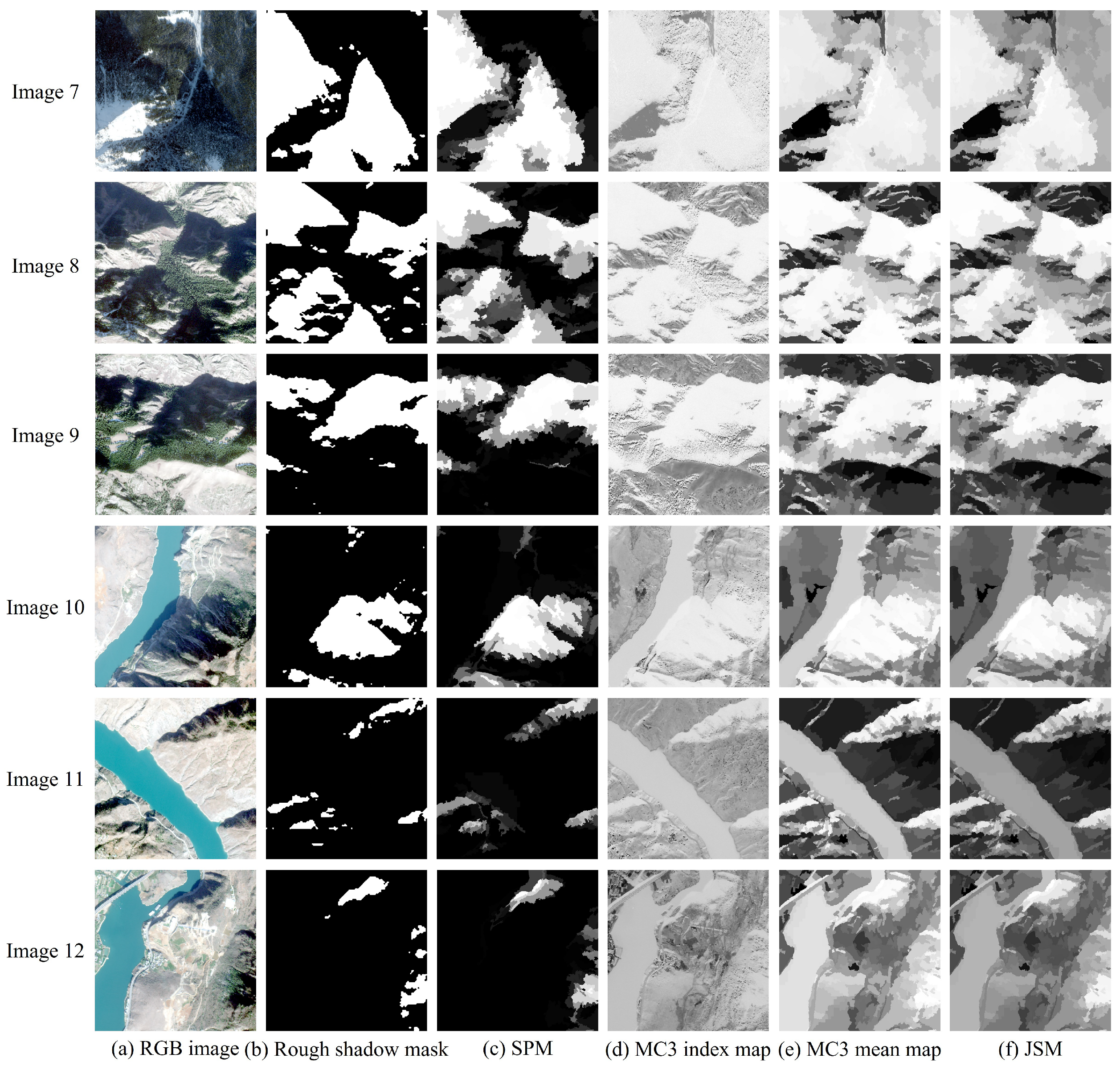
The corresponding ground truth images are shown in Figure 12b. The detection results of Silva, Wang, Zhou, Guan, ECA, MC3, and CTS are shown in Figure 12c–i, respectively. Figure 13 illustrates the process diagrams of CTS for six images. The quantitative evaluation results of the seven methods are summarized in

Table 4. Quantitative evaluation results of shadow detection.

Image	Method	${\mathit{P}}_{\mathit{s}}$ (%)	${\mathit{P}}_{\mathit{n}}$ (%)	${\mathit{U}}_{\mathit{s}}$ (%)	${\mathit{U}}_{\mathit{n}}$ (%)	${\mathit{E}}_{\mathit{c}}$ (%)	${\mathit{E}}_{\mathit{o}}$ (%)	$\mathit{\tau }$ (%)	$\mathit{kappa}$
7	Silva	89.38	26.48	54.29	71.84	73.52	10.62	57.56	0.16
	Wang	97.86	19.37	54.25	90.26	80.63	2.14	58.15	0.17
	Zhou	90.12	37.24	58.38	79.41	62.76	9.88	63.37	0.27
	Guan	94.79	41.49	61.28	89.07	58.51	5.21	67.83	0.36
	ECA	97.49	84.55	86.04	97.18	15.45	2.51	90.94	0.82
	Ours (MC3)	95.67	68.48	74.78	94.18	31.52	4.33	81.92	0.64
	Ours (CTS)	91.41	96.41	96.13	91.99	3.59	8.59	93.94	0.88
8	Silva	99.27	63.43	73.68	98.83	36.57	0.73	81.63	0.63
	Wang	98.70	61.22	72.41	97.86	38.79	1.30	80.25	0.60
	Zhou	98.85	69.65	77.06	98.33	30.35	1.15	84.48	0.69
	Guan	96.32	83.71	85.91	95.66	16.29	3.68	90.11	0.8
	ECA	92.86	89.72	90.30	92.42	10.28	7.14	91.31	0.83
	Ours (MC3)	98.42	72.18	78.49	97.80	27.82	1.58	85.50	0.71
	Ours (CTS)	95.86	89.74	90.59	95.45	10.26	4.14	92.84	0.86
9	Silva	99.96	60.98	49.20	99.97	39.02	0.04	71.67	0.46
	Wang	99.78	66.10	52.67	99.87	33.90	0.22	75.34	0.52
	Zhou	99.62	79.69	64.98	99.82	20.31	0.38	85.16	0.68
	Guan	93.12	95.83	89.41	97.36	4.17	6.88	95.09	0.88
	ECA	88.08	98.16	94.77	95.61	1.84	11.92	95.39	0.88
	Ours (MC3)	98.00	89.13	77.32	99.16	10.87	2.00	91.56	0.80
	Ours (CTS)	95.19	96.79	91.80	98.16	3.21	4.81	96.35	0.91
10	Silva	91.86	78.45	57.41	96.82	21.55	8.14	81.67	0.58
	Wang	98.40	70.29	51.16	99.29	29.71	1.60	77.04	0.52
	Zhou	97.59	74.53	54.78	98.99	25.47	2.41	80.07	0.57
	Guan	92.80	96.25	88.67	97.69	3.75	7.20	95.42	0.88
	ECA	88.83	98.56	95.11	96.54	1.44	11.17	96.22	0.89
	Ours (MC3)	97.14	79.29	59.74	98.87	20.71	2.86	83.58	0.63
	Ours (CTS)	92.08	98.11	93.89	97.51	1.89	7.92	96.66	0.91
11	Silva	76.52	75.85	24.18	96.98	24.15	23.48	75.91	0.27
	Wang	94.46	71.62	25.09	99.23	28.38	5.54	73.71	0.29
	Zhou	90.68	74.53	26.38	98.76	25.47	9.32	76.01	0.31
	Guan	65.77	99.16	88.71	96.64	0.84	34.23	96.11	0.73
	ECA	63.72	99.64	94.66	96.46	0.36	36.28	96.35	0.74
	Ours (MC3)	93.31	77.67	29.60	99.14	22.33	6.69	79.10	0.36
	Ours (CTS)	86.87	99.16	91.19	98.68	0.84	13.13	98.03	0.88
12	Silva	73.44	76.83	23.83	96.70	23.17	26.56	76.52	0.26
	Wang	49.09	73.51	15.46	93.60	26.49	50.91	71.32	0.11
	Zhou	93.42	74.96	26.91	99.14	25.04	6.58	76.62	0.32
	Guan	72.62	98.60	83.70	97.33	1.40	27.38	96.27	0.76
	ECA	42.68	99.10	82.32	94.60	0.90	57.32	94.03	0.53
	Ours (MC3)	96.03	68.84	23.32	99.43	31.16	3.97	71.28	0.27
	Ours (CTS)	92.87	97.46	78.30	99.28	2.54	7.13	97.05	0.83

Note: The values in bold indicate the best performance.

.

The CTS method, by analysis of the DEM, is able to correctly identify shadows cast on the ground by upland targets without confusion between shaded and non-shaded dark features due to spectral similarity. As shown in Figure 13b, the shadow regions in the rough shadow mask are all approximately accurate and do not contain vegetation and water bodies. Therefore, the vegetation and water body regions have almost no superpixels containing shadow pixels in the rough shadow mask. As shown in Figure 13c, the SPM has almost zero value for the background regions and the highest value for the shadow regions. However, in Figure 13e, the values of the vegetation and water body superpixels are close to the shadow values in the MC3 mean map.

After the SPM is fused with the MC3 mean map with certain weights, as shown in Figure 13f, the values of the background superpixels in the JSM are pulled down so that the difference between the shadow superpixels and the vegetation and water body superpixels is enlarged. The addition of the DEM rough shadow mask widens the difference between shadows and dark features. Therefore, applying the multi-level Otsu method for a histogram threshold segmentation of the JSM can delineate shadows and the background more accurately.

4. Discussion

4.1. Experimental Results Analysis

The shadow detection results of Images 3–6 demonstrate that Silva’s method has a large area of misdetection in general, which is especially obvious in Images 4–6. Moreover, it produces some discrete false alarms with fragmented shadow edges, which is caused by its direct single-pixel calculation of the shadow index and application of threshold segmentation. Wang’s method is able to ensure the continuity of shadows by virtue of superpixel segmentation. However, it has some omissions, and some shadows have inwardly concave edges. Zhou’s method exhibits a relatively high rate of misdetection, and due to its sole reliance on the NIR band, it fails to differentiate between water bodies and shadows in Image 4. The Guan and ECA methods have some shadow omissions in Images 3–6, and the shadow boundaries are blurred. Our MC3 method has very few shadow misdetections and omissions on the four images and can ensure the complete detection of large and small shadows with smooth and clear shadow boundaries. The quantitative evaluation results also demonstrate the superiority of MC3 with an average overall accuracy of 94.03%, which is an improvement of 21.82%, 6.77%, 2.29%, 2.54%, and 2.74% compared to the Silva, Wang, Zhou, Guan, and ECA methods, respectively. Its higher $P_s$ and $U_n$ and lower $E_o$ demonstrate its ability to effectively recognize shadows.

In the shadow detection results of Images 7–12, both Silva and Wang’s methods recognize vegetation and water bodies as shadows. Compared to those, Zhou’s method effectively mitigates vegetation misdetection by virtue of the large difference in brightness between vegetation and shadows in the NIR band, but it still cannot avoid the misdetection of water bodies as shadows. Guan’s method does not show any case of vegetation and water bodies being misdetected as shadows in the other five images except for Image 7 because it recommends error-prone dark regions through the Dark-Region Recommendation (DRR) module. However, at the same time, it also excludes brighter shadow regions, such as the hillside shadow on the left side of the river in Image 11 and the thin shadow cast by the bridge across the river in Image 12. The ECA method does not have too many shadow misdetections in any of the six images, but there are more shadow omissions, such as the hillside shadow on the right side of Image 12. The MC3 method, like Silva, Wang, and Zhou, has many shadow misdetections due to the presence of dark vegetation and water bodies. This exemplifies the drawbacks of only using spectral features to detect shadows, where large dark objects in the image can make shadow recognition more difficult. Our CTS is able to exclude dark vegetation and water bodies from interfering with shadow recognition. In addition to correctly detecting hillside shadows, CTS also ensures that the small and non-terrain-induced shadows can be detected, such as the small patch of shadows above Image 10 and the shadows of the bridge in Image 12. Thus, the shadows detected by CTS are both real and complete and are generally consistent with the results of visual interpretation.

The quantitative evaluation results provided by Table 4 also show that CTS performs best among the seven methods. The average overall accuracy is 95.81%, which is 21.65%, 23.18%, 18.19%, and 13.65% higher than the Silva, Wang, Zhou, and MC3 methods, respectively. The kappa coefficients of all six images remain above 0.8. Compared with other traditional methods, the committed error of CTS is significantly lower, basically staying around 2%, whereas the others are 20% or more. On the six images, CTS achieves a mean overall accuracy of 95.81% compared with 90.14% for Guan’s method and 94.04% for ECA. CTS maintains a high overall accuracy over multiple images compared to Guan’s model and ECA, which shows that CTS is also the most robust.

The MC3 method behaves better on Images 3–6 (the average overall accuracy is 94.03%) but worse on Images 7–12 (the average overall accuracy is 82.16%). This may be due to the fact that there are fewer dark features affecting shadow extraction in Images 3–6, whereas the opposite is true in Images 7–12. Large areas of dark vegetation and water bodies make it more difficult to accurately extract shadows. Generally, the shadows in urban area images are mainly building shadows, and the areas of vegetation and water bodies are smaller compared to mountainous images. So it is perfectly fine for MC3 to be applied to urban area images.

The CTS method needs to be used in conjunction with DEM corresponding to the images, and its advantages become apparent when there are large areas of dark objects that hinder the extraction of true shadows. In our CTS experiment, we used the DEM with a resolution of 12.5 m, which is open-source and relatively easy to obtain. In the DEM-based shadow coarse detection experiment, the detection performance between the 30 m DEM and the 12.5 m DEM showed little difference, and the gap became even smaller after generating the SPM. Therefore, the impact of the resolution of the DEM on CTS detection performance can be considered negligible. If high-resolution urban DEMs are available, CTS can also be used in urban areas. However, high-resolution DEMs are difficult to obtain, as they typically need to be generated from the original low-resolution DEM combined with panchromatic stereo images of optical images, which involves relatively high thresholds and costs.

4.2. Parameters Analysis

CTS can distinguish well between shadows and dark ground objects in images, avoiding the shortcomings of MC3, which only utilizes spectral features. However, there are still some factors that may lead to inaccurate detection results:

(1)

The number of over-segmented superpixels $n_o$.

The multi-scale segmentation of images ensures the continuity and integrity of shadows, but it may still face a situation where shadows and non-shadows are mixed within the same object, especially for fine shadows and shadow edges. When the $a_m$ is certain, this situation is related to $n_o$. If $n_o$ is too small, the resulting superpixels are more likely to contain both shadows and non-shadows; if $n_o$ is too large, the difference between shadow superpixels and non-shadow superpixels is not significant enough, meaning that they are more likely to be merged into the same object. Therefore, a suitable $n_o$ can avoid the problem as much as possible. Incorporating shadow features into superpixel segmentation similarity metrics may be able to fundamentally solve the problem, which will be studied in our future work.

(2)

The weight of the DEM rough shadow mask $w_{\mathrm{dem}}$.

The fusion weights of the SPM and the MC3 mean map are also particularly important to the detection results. The overall accuracy $\tau$ changes in Images 7–12 under different $w_{\mathrm{dem}}$ are illustrated in Figure 14. The overall accuracy for all six images reaches its highest at $w_{\mathrm{dem}}=0.2$, which basically stays around 95%. When $w_{\mathrm{dem}}$ tends to 0 or 1, i.e., only the MC3 mean map or only the SPM is considered, the overall accuracy decreases. It falls below 75% at $w_{\mathrm{dem}}=0$ in Images 7, 11, and 12, and Image 8 also falls to 75% at $w_{\mathrm{dem}}=1$. Therefore, it can be seen that adding the terrain factor has a positive enhancement effect on image shadow detection, confirming the good performance of CTS.

(3)

The number of multi-thresholds c.

When performing histogram thresholding segmentation, the setting of the number of multi-thresholds c is also an important factor that affects the detection accuracy. If c is too small, it can result in dark objects, such as vegetation, water bodies, and soil, close to shadows being classified as shadows; if c is too large, it can lead to true shadows being missed. Figure 15 shows the overall accuracy changes of the six images under different c. When $c=1$, the $\tau$ is very low for all six images, whereas when $c=2$, the $\tau$ improves drastically. For Image 8, when $c>3$, the overall accuracy decreases, indicating that a threshold that is too high leads to partial shadow misdetection. Therefore, in this paper, the number of multi-thresholds c is set to 3 when performing CTS.

4.3. Process Speed

The experiments were conducted on a Windows 11 system equipped with an Intel Core i5-14900 CPU (Intel Corporation, Santa Clara, CA, USA), an NVIDIA GeForce RTX 4060 Ti GPU with 12 GB memory (NVIDIA Corporation, Santa Clara, CA, USA), and 16 GB of RAM. The implementation was carried out using PyTorch 1.12.0 and MATLAB R2020a.

Table 5. The average detection time of five methods.

Method	Detection Time (s)
Silva et al. [20]	0.20
Wang et al. [22]	6.89
Zhou et al. [18]	1.98
Guan et al. [34]	3.46
Fang et al. [35] (ECA)	1.57
Ours(MC3)	0.84
Ours (CTS)	0.97 (DEM rough shadow mask)
	0.91 (shadow detection perform)

presents the average detection time of the seven methods for all images.

Silva’s method has the shortest time of 0.2 s, and Wang’s method has the longest time of 6.89 s. Our MC3 takes less time than the Wang, Zhou, Guan, and ECA methods. CTS consists of two parts: generating a DEM rough shadow mask and performing shadow detection. In principle, when generating the rough shadow mask, the shade analysis radius needs to be calculated for each grid point. However, through extensive experiments, we found that for a $512\times 512$ image, the local shade analysis radius $r_l$ generally does not exceed 3000 m. Therefore, we can uniformly set $r_l=3000$ m without the need to calculate it for each individual point, which helps to save program runtime. The average runtime for generating the rough shadow mask is 0.97 s, and the average time for shadow detection is 0.91 s. So, CTS requires 1.88 s per image on average versus 3.46 s for Guan’s model and 1.57 s for the ECA. This demonstrates that our proposed methods, MC3 and CTS, also perform better in terms of process speed.

5. Conclusions

In this paper, we propose a DEM-based shadow coarse detection method, an MC3-based shadow fine detection method, and a shadow detection method combining topography and spectra (CTS) for remote sensing images in mountainous environments. The DEM-based shadow coarse detection method obtains a rough shadow mask corresponding to the image by utilizing DEM data and the Sun’s position at the moment of image acquisition. The MC3-based shadow fine detection method includes image enhancement with linear and logarithmic stretching, multi-scale superpixel segmentation (FNEA based on SLIC), and MC3 index calculation. The CTS method takes the superpixel as a bridge connecting the DEM rough shadow mask and the MC3 index map, and the fusion map can reflect the probability of superpixels belonging to shadow both topographically and spectrally. After the experiments of three shadow detection methods on several images, the following three conclusions can be drawn:

(1)

The DEM-based shadow coarse detection method can locate the main shadow region in images. Compared with the 12.5 m and 30 m DEMs, the shadow extracted by 5 m DEM is more refined and has a better fit with the original image. The shadow extracted by the 30 m DEM is slightly coarser than 12.5 m, but it does not affect the effectiveness of the DEM method in locating the main shadow regions.

(2)

The MC3-based shadow fine detection method extracts shadows in the image meticulously and completely. It can avoid the problem of dark objects being mistakenly detected as shadows to some extent. Compared to the methods proposed by Silva, Wang, Zhou, Guan, and Fang (ECA), the MC3-based approach demonstrates superior performance across most evaluation metrics, with a significant reduction in omitted errors. The overall accuracy and kappa coefficient have reached the best among the six methods.

(3)

The CTS method can accurately recognize shadows and avoid the misdetection of dark objects, such as vegetation and water body. The method obtains a Joint Shadow probability Map (JSM) by combining the Shadow pixel Proportion Map (SPM) and the MC3 mean map, and it utilizes both topographic and spectral factors to make the distinction between shadows and dark objects more obvious. The experiments confirm that the detection performance of CTS is further improved on the basis of the MC3-based method.

In the future research work, we will conduct more experiments on the other sources of DEM data (e.g., Lidar) or time-sensitive data to assess the robustness and applicability of our methods. We have compared CTS with CNN-based deep learning methods, and in the future, we can compare it with GAN-based deep models to observe its accuracy and robustness. In addition, CTS is also fully applicable to urban areas if high-resolution DEMs of urbanized areas are obtained, which has the immediate effect of separating the shadows of buildings from the urban greenery and artificial lakes.