1. Introduction
Wave tanks are essential facilities for conducting fluid dynamics experiments that explore the interaction between water waves and structures. One side of the tank is usually fitted with a wave generator to create waves defined by the user. However, if the wave absorber on the opposite side of the tank is inadequately designed, it may cause undesirable reflections that deteriorate the reliability of the experiments, and cause delays in the experiment owing to the waiting time needed for disappearing residual waves in a tank after the wave generator is stopped. Depending on the size of the wave tank, wave absorbers of different shapes and materials are utilized. Porous plates, known for their effectiveness in dissipating wave energy and minimizing wave reflections, are commonly employed as passive wave absorbers. The authors in [
1] reviewed and investigated existing wave absorbers in 48 wave basins around the world. According to the report, wave absorbers utilizing porous plates are predominantly categorized into vertical, horizontal, and inclined types. Vertical wave absorbers necessitate several porous plates with gradually reducing porosity to attain the desirable wave absorption efficiency. Therefore, this configuration requires substantial installation space and frequently results in resonance between the plates.
Horizontal porous plates have demonstrated exceptional effectiveness in dissipating wave energy, making them useful for coastal protection and improving harbor calmness. Studies referenced in [
2,
3] explored the performance of horizontal porous plates through the boundary element method (BEM) and the matched eigenfunction expansion method (MEEM), respectively. The energy dissipation capacity of horizontal porous plates largely depends on their porosity. This energy dissipation is considered by the porous boundary condition, particularly Darcy’s model [
3,
4,
5,
6,
7], which outlines the linear correlation between velocity and pressure drop. In ref. [
5], the authors developed an analytical model for wave-absorbing systems based on Darcy’s model. Their analytical solution using a MEEM, and their numerical solution using a multi-domain BEM, were validated through a series of experiments. These research findings indicate that the optimal values for wave absorption efficiency are a slope angle of 10° and a plate porosity of 0.1. Additionally, the local shape of the porous plate (e.g., slits, circular holes, rectangular holes, etc.) was found to have no significant impact on energy dissipation [
5,
8,
9]. As an alternative energy dissipation model, several authors have considered the quadratic relationship between pressure drop and velocity. The authors in [
10] were the first to derive an expression for long-wave head loss in porous walls. Several authors in articles [
11,
12] extended the work of those in ref. [
10] to investigate wave interactions with porous plates. The authors of [
13,
14] examined energy dissipation through porous plates by employing an equivalent quadratic velocity model that incorporates both inertial and drag effects. Subsequently, another article [
15] examined wave energy dissipation caused by a horizontal slotted plate using a quadratic velocity model with a CFD-determined drag coefficient. They validated their findings by comparing them with CFD-based numerical simulations and experimental results.
The boundary element method (BEM) has been effectively utilized in wave problems due to its distinct advantages over other domain-based methods such as the Finite Difference Method (FDM) and Finite Element Method (FEM). The BEM reduces the problem’s dimensionality by one order, simplifying calculations and enhancing accuracy through its integral formulation. Numerous researchers have extended the application of the BEM to study wave interaction with porous structures [
5,
16,
17,
18,
19]. When we apply a BEM to a boundary-value problem (BVP) with a zero-thickness plate in a numerical domain, the standard single-domain BEM has difficulty in guaranteeing a unique solution due to rank deficiency. For unique solutions to these BVPs, we must depend on the multi-domain BEM or the dual boundary element method (DBEM), including the hyper-singular integral formulation. In ref. [
20], the authors developed the DBEM to address the rank deficiency problem inherent in standard BEM. The core concept of DBEM is to resolve the rank deficiency by employing hyper-singular boundary integral equations, thereby leading to a full DBEM formulation. Several researchers applied the DBEM to investigate the hydrodynamic performance of water waves over zero-thickness barriers [
21,
22,
23,
24,
25,
26,
27]. The article [
22] used the DBEM to analyze the interaction between zero-thickness immersed barriers and normally incident waves. The authors in [
23] developed the DBEM for modified Helmholtz equations to evaluate the hydrodynamic performance of bottom-fixed thin vertical barriers in oblique incident waves. Article [
24] extended the DBEM to treat immersed thin vertical and inclined wave barriers. The authors in [
25] employed the DBEM to solve the scattering problem involving a locked horizontal zero-thickness wave barrier and compared the results with a finite-thickness wave barrier using a standard BEM. Additionally, the numerical results from both two BEM approaches were compared with experimental measurements. The authors of [
28] investigated the inclined single porous and dual parallel porous plates to develop an efficient wave absorber using a DBEM. The self-conducted experiment validated the numerical solutions. It was found that an inclined single porous plate proved to work well as a competitive wave absorber when compared to the dual parallel plates.
Machine learning is becoming increasingly popular for optimizing design parameters in engineering applications. Artificial neural network (ANN) models are especially widely adopted as promising machine learning (ML) models because they can learn complex patterns/relations and make accurate predictions. It is modeled after simplified representations of biological neurons in the brain and consists of interconnected nodes, where each circular node represents an artificial neuron, and the arrows represent the connections between the input and output. With multiple hidden layers, ANN models allow the neural network to identify and interpret complex relationships between input and output features in the data. Thus, it is a powerful tool for applications involving intricate data patterns and relationships. In ref. [
29], the authors employed an ANN model to optimize the design of a multilayer porous wave absorber. The porosity and submergence depth of the topmost plate were identified as the key design parameters, with their optimal ranges specified. Article [
30] employed a machine learning approach for designing and additively manufacturing porous sound absorbers, utilizing two models: an artificial neural network and a k-nearest neighbor algorithm. The results showed that both models could accurately predict design parameters. A deep learning-based framework is developed in [
31] for designing random porous metal structures with a focus on maximizing energy absorption. The authors of [
32] proposed a simple approach to controlling plunger wavemakers using an ML approach with a neural network model. Article [
33] used an ANN model to actively control the absorption of random waves in a wave flume. The authors of [
34] utilized machine learning models to incorporate nonlinear viscous damping for a heave disk with specified porosities in the time domain. Four different ML models—decision tree, random forest, support vector machine, and neural network—were employed and trained to predict the drag coefficient based on disk porosity and the Keulegan–Carpenter (KC) number as input features. In a different study [
35], the authors assessed the performance of the Savonius hydrokinetic turbine using soft computing techniques such as CatBoost, ANN, Random Forests (RFs), Multivariate Adaptive Regression Splines (MARSs), Adaptive Neuro-Fuzzy Inference System (ANFIS), and several hybrid ANFIS models (ANFIS-GA, ANFIS-SMA, and ANFIS-MPA), along with Linear Regression (LR). They aimed to predict the power coefficient and evaluate the impact of input parameters on the turbine’s performance. Most of the methods successfully predicted the power coefficient with acceptable accuracy. Articles [
36,
37,
38,
39] presented optimization using genetic algorithms, highlighting techniques and applications across various domains. These include solving multi-objective problems, optimizing wave energy converter array layouts, image optimization, and techno-economic optimization. Articles [
40,
41,
42] utilized support vector machines for optimization across a range of domains.
A comprehensive review of computational intelligence techniques was carried out in [
43], including neural, fuzzy, and evolutionary computations, applied to applications of wave energy. Their review covered the estimation of resources as well as the control and design and control of wave energy converters (WECs). Most applications of neural computation techniques focused on predicting various parameters of wave energy with the multilayer perceptron (MLP) algorithm. The MLP is a type of ANN with multiple layers of neurons. This algorithm is based on a feedforward neural network with training performed using the error backpropagation method. The authors in [
44] used an MLP regression of the ANN model to optimize the design of an asymmetric WEC to optimize the average extracted power.
The multi-criteria decision analysis (MCDA) is a decision-making framework used to evaluate and prioritize multiple conflicting criteria. The weighted sum model (WSM) is a quantitative decision-making tool used in multi-criteria decision-making approach to evaluate and prioritize different alternatives based on multiple criteria. The authors in [
45] conducted a multi-criteria site selection for offshore renewable energy platforms using WSM. Specialized decision-support tools have been developed to facilitate flexible, multi-criteria site selection for combined wind–wave energy platforms, with a focus on available energy resources. WSM has been employed in [
46] to determine special allocation funds recipients. This method effectively generates rankings among the proposed alternatives in a special allocation fund. Article [
47] used the WSM in titanium alloy selection for biomedical applications. The developed methodology was recognized for its applicability across various applications.
This study aims to optimize design parameters related to a wave absorber with an inclined porous plate to reduce the reflected waves while also reducing the spatial footprint of the porous plate. To achieve this, a computationally efficient and technically robust optimization framework is developed by integrating the dual boundary element method (DBEM), artificial neural networks (ANNs), and the weighted sum model (WSM) within a multi-criteria decision analysis (MCDA) framework. This ensemble approach facilitates objective-driven design and supports informed decision-making in the context of ocean engineering. The Boundary Value Problem (BVP) was formulated and solved using the DBEM, which addresses two distinct boundary integral equations—singular and hyper-singular—at coincident source points along each side of the degenerate boundary. The design parameters affecting the performance of an inclined porous wave absorber are the porosity, inclination angle, and length of a porous plate. In the present study, porosity is excluded from design parameters because the optimal porosity has already been clarified to be around 0.1 in previous articles [
5,
15,
28]. Thus, the optimal values for the inclination angle and plate length can minimize wave reflections from the walls of the wave basin while simultaneously reducing the spatial footprint. The MLP regression algorithm of the ANN model is used to determine the optimal design parameters. This approach significantly reduces the need for complex and time-consuming numerical calculations while efficiently identifying the best optimal design parameters. This supervised learning method derives insights through a dataset used in training. In the present study, the inclination angle and non-dimensional plate length have been adopted as input features, and the averaged reflection coefficient as an output feature. The training dataset of the given input features and the corresponding output feature was generated using the DBEM. The trained ANN model was subsequently used to predict the averaged reflection coefficient using a larger dataset comprising a combination of design parameters. During the optimization process to minimize both reflected waves and spatial footprint, the weighting factors are assigned based on their relative importance to each other, employing the weighted sum model (WSM) within the multi-criteria decision-making approach.
2. Boundary Value Problem (BVP)
Let us consider an inclined porous plate fixed at the end wall of a two-dimensional wave flume in the water depth of
. The length of a porous plate is
and the inclined angle
. The coordinates
with the
axis pointing vertically upward may be chosen. The incident waves of frequency
and amplitude
propagate from
. For an inviscid irrotational flow, the velocity
can be expressed as the gradient of a scalar potential
. The conservation of mass requires that the potential satisfies Laplace’s equation.
and under the assumption of the small amplitude wave, the boundary conditions are listed below.
where
is the gravitational acceleration.
Sharp constriction on the porous plate makes flow separate downstream and vortices are formed from adjacent holes to create eddy zones. Therefore, boundary conditions at the porous plate are needed to realize energy dissipation by these vortices. The authors of [
10] established the following boundary conditions.
where
denotes the modulus of the complex number.
The above equations provide the matching conditions on the porous plate’s upper (+) and lower (−) sides. The drag coefficient representing energy dissipation and inertial coefficient are determined empirically. The inertial term can be disregarded when the porous plate is thin and the hole size is small ().
The drag coefficient for a porous plate featuring uniformly distributed circular holes was empirically determined as a function of porosity using CFD simulations (Star-CCM+) for channel flow through the circular holes [
15,
48].
In steady flows with a high Reynolds number past sharp-edged orifices, the discharge coefficient depends primarily on the porosity.
For simple harmonic motion with frequency
, the linearity of the BVP allows the separation of the time factor
as follows:
The linearized BVP including the radiation condition can be reduced to
where the wave number
and frequency
are related by the dispersion relation
.
The incident wave potential
with the wave amplitude
propagating from
is given by
The quadratic drag term in Equation (6) makes the entire problem nonlinear, and the response to a simple harmonic
input should contain many harmonics (
,
,...). By employing equivalent linearization that the response is dominated by the first harmonic, the boundary conditions on the porous plate can be expressed as follows:
where
denotes the equivalent drag coefficient.
Rather than using the quadratic velocity model mentioned above, the flow past a thin porous plate can alternatively be assumed to follow linear Darcy’s model, where the normal velocity of fluid flow is linearly proportional to the potential jump.
where
, called the porosity parameter, was determined empirically in article [
5]’s experiments.
4. ANN Modeling
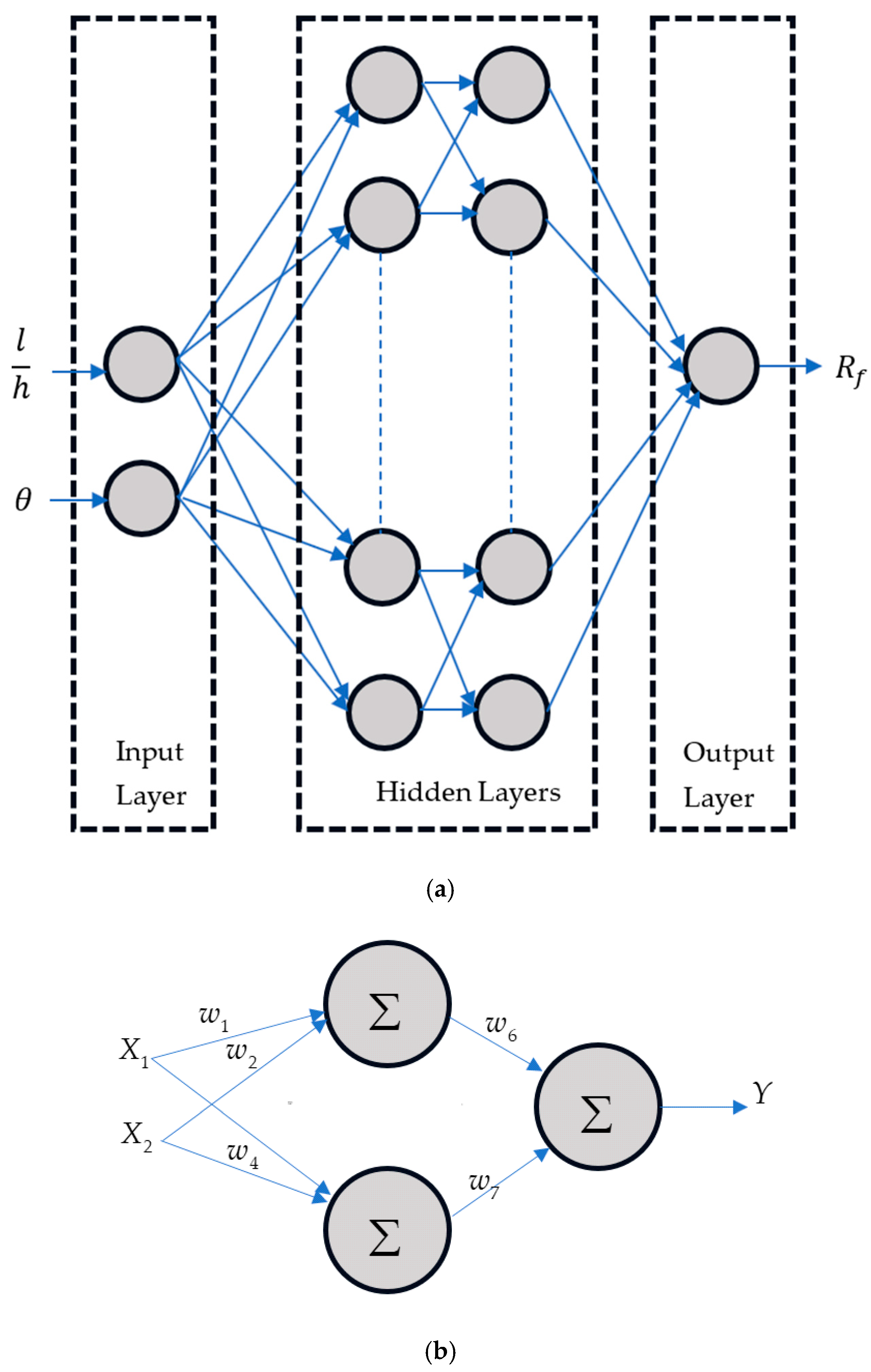
An artificial neural network (ANN) model was applied to identify the optimal design parameters of the inclined porous plate as a wave absorber. The ANN model has the advantage of learning complex nonlinear relationships, handling complex data, and parallel-processing capability. This study utilizes the multilayer perceptron (MLP) regression algorithm of the ANN model, a supervised learning algorithm that trains on a labeled dataset. This algorithm possesses strong nonlinear mapping capabilities, enabling it to make accurate predictions. The neural network architecture is flexible, allowing for adjustments in the number of hidden layers and neurons in each layer to tailor the model training to the research and training goals.
The ANN model includes an input layer with two input features such as non-dimensional plate length (
) and inclined angle (
), several hidden layers, and an output layer with a single output feature of averaged reflection coefficient (
,
= total number of incident wave periods). Another important parameter affecting the reflection coefficient is the porosity of an inclined porous wave absorber. However, it is excluded from the input features because previous articles have already clarified that the optimal porosity is around 0.1 [
5,
15,
28].
Figure 2 illustrates the architecture of the ANN model and the mapping of input and output with its weights (
) and activation function (
) of artificial neurons. Each layer is composed of nodes or artificial neurons that are interconnected, each with its activation function. Each node in the network has its weight and threshold. When the node’s output surpasses the specified threshold, it is activated and transmits data to the next layer of the network. If not, the data are not passed on to the next layer. The activation function of a neural network is crucial for activating the neurons of the hidden layer, enabling them to generate preferable outputs and inhibiting nonlinearity in the model. The performance of the neural network model is affected by several hyperparameters, including the number of hidden layers, the number of neurons in each layer, batch size, learning rate, regularization parameters, solver, activation function, and the number of epochs. Optimizing these hyperparameters can significantly enhance the training rate of the ANN model and improve its prediction accuracy.
Figure 3 illustrates all the processes involved in ANN modeling and predictions. Specifics of the tasks are outlined in the following sections.
4.1. Preparation of Training Dataset
The ANN model must be trained using a set of training samples that include input features and their corresponding known output features. As a supervised machine learning algorithm, the ANN relies on labeled datasets to effectively train the model, enabling it to predict outcomes and recognize patterns. Therefore, the sample dataset for training is generated utilizing the DBEM model for the input features of plate length (), and inclined angle () with an output feature of averaged reflection coefficient (). The other parameters such as water depth (), porosity (), and wave steepness () are fixed.
Choosing the appropriate sampling method is essential for training the ANN model. An effective sampling method ensures a more balanced distribution of samples, which enhances the neural network’s training and improves the model’s accuracy. To create random sample points, the Latin Hypercube Sampling (LHS) method is used. This approach provides advantages like reducing variance and efficiently giving a comprehensive datapoint representation of the parameter space. Consequently, this method has been used by several studies [
29,
34,
44,
49,
50]. The sample set, which includes two input features, is as follows:
Using LHS, the input sample set of 300 instances is generated, with a scatter plot of these samples displayed in
Figure 4. Each input feature covers the entire sampling space, ensuring a thorough representation throughout the range.
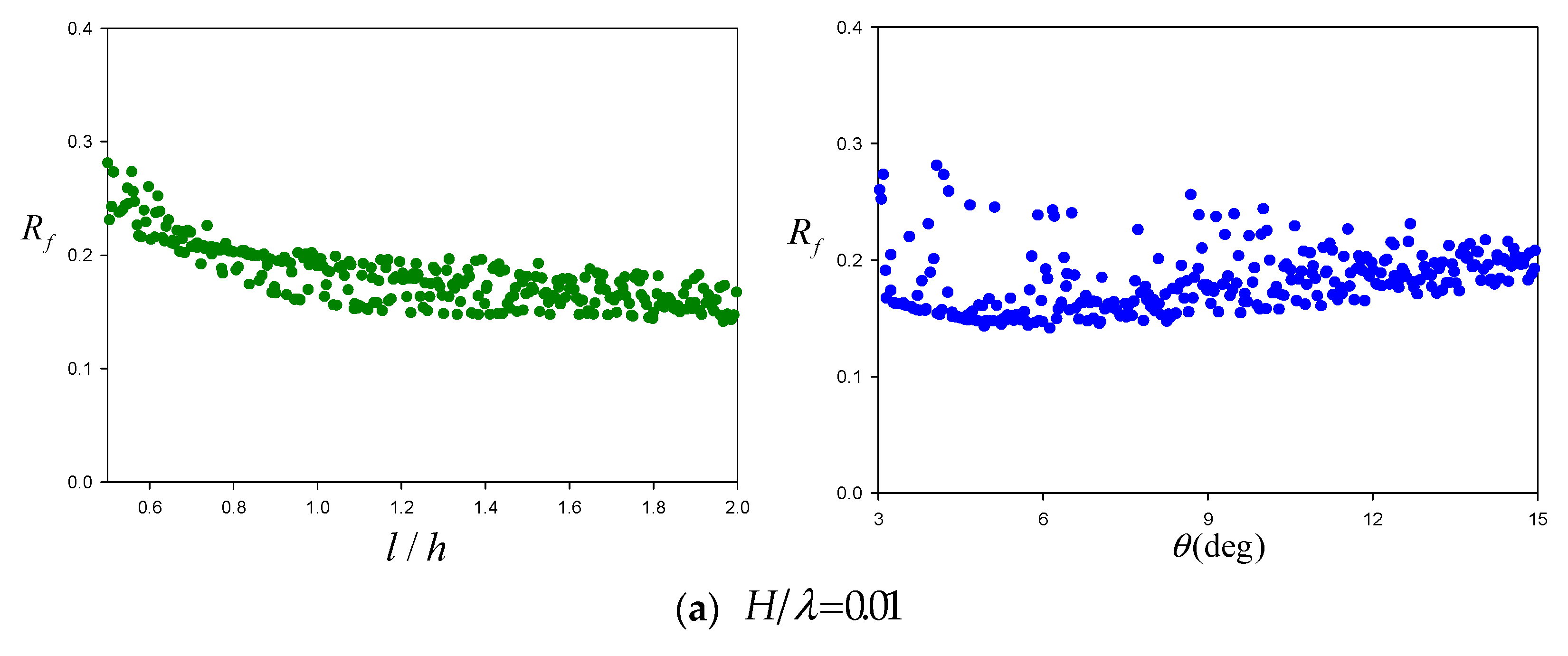
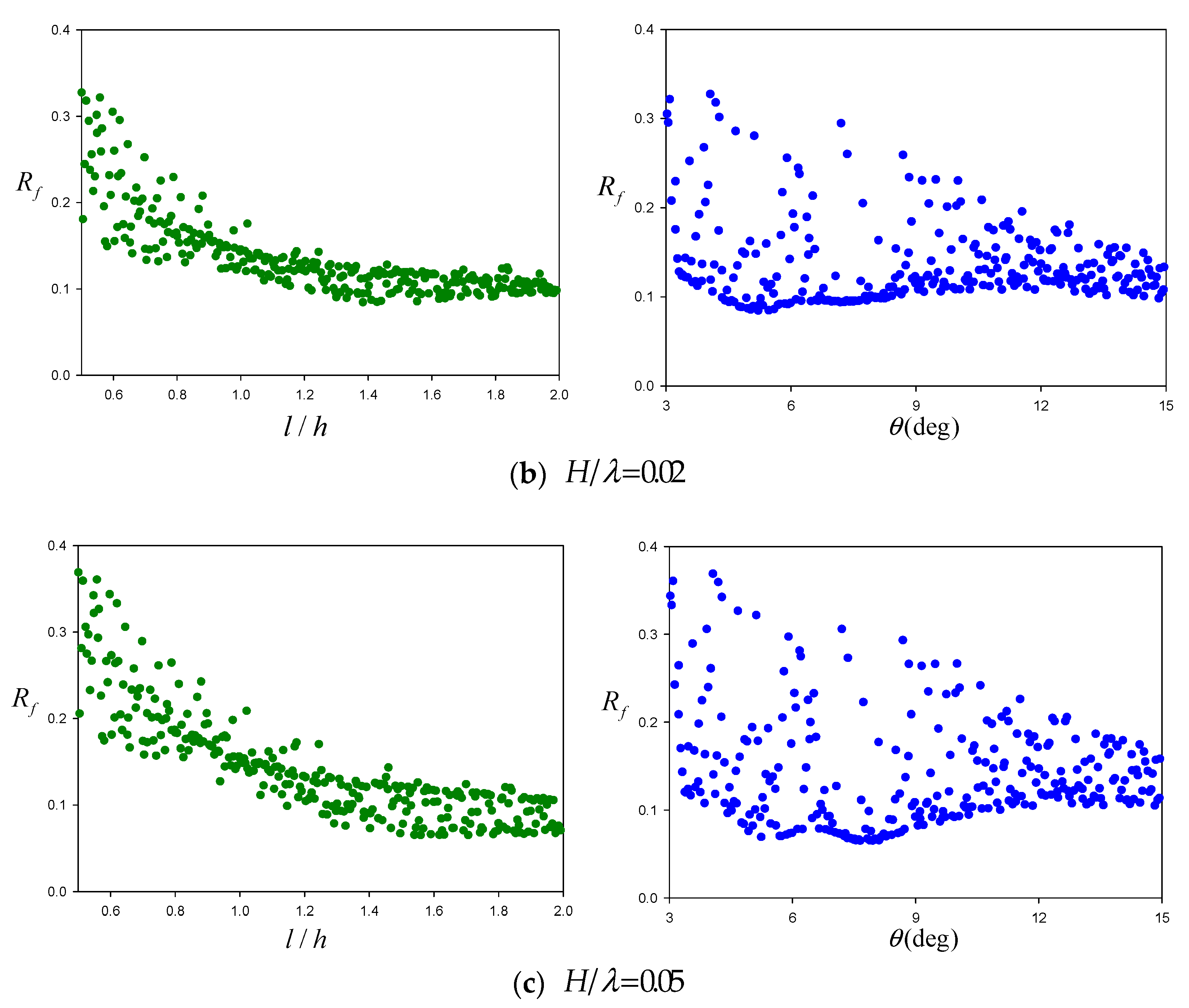
The correlation between input features and the output was assessed to understand how each input influenced the result for three different wave steepness (
).
Figure 5 shows scatter plots of non-dimensional plate length and inclined angle against the averaged reflection coefficient for different wave steepness. The plots show that increasing the plate length significantly reduces the averaged reflection coefficient up to the mid-range of the plate length, after which a gradual decrease is observed. The effect of the inclined angle on the averaged reflection coefficient is somewhat scattered, with the minimum value occurring around 5° to 8°.
4.2. Data Preprocessing
The full dataset is split into training, validation, and test subsets. The training and validation subsets are used to train the ANN model, while the test subset is reserved for performance evaluation. Of the 300 data points, 64% are allocated for training, 16% for validation, and 20% for testing. The allocation of data points is carried out randomly. The input features in the current database may vary widely, potentially affecting the performance of the ANN model. Therefore, it is essential to normalize the input features to a defined range. This normalization is performed using the MinMaxScaler, which individually scales and transforms each input feature within a specified range based on the training set. This process helps train the model for quicker learning and faster convergence. The formula for the min–max scaling is given by
Here, ‘min’ and ‘max’ refer to the minimum and maximum values within the range of the input feature. For each feature, the minimum value is scaled to 0, the maximum value is scaled to 1, and all other values are adjusted to fall between 0 and 1. This normalization process was uniformly applied to all variables.
4.3. ANN Model Initialization
The ANN model must be initialized with appropriate hyperparameters before training, as these parameters significantly affect the model’s performance. As shown in
Figure 3, the training process begins with an initial set of hyperparameters. The training subset is used to train the model, while the validation data are employed for evaluation. The training process proceeds by adjusting the hyperparameters using a random search algorithm until the stopping criteria are met. Here, the stopping criteria achieved a higher
score with minimal MSE and MAE values. The optimization process is explored with the following parameters: number of hidden layers {2,3,4}, number of neurons in each hidden layer {5,10,15,20,25,30,40}, learning rate {0.1,0.05,0.01,0.001,0.0001}, regularization parameter {0.1,0.001,0.0001,0.00001}, epochs {500,1000,1500}, activation function {Identity,Logistic,Tanh,ReLU}, and solver {LBFGS,SGD,ADAM}. After extensively trying various combinations of hyperparameters, the optimal hyperparameters are listed in
Table 1.
The nonlinear activation function, Rectified Linear Unit (ReLU), is used, defined as , where x is the input to the neuron. Information flows from the input layer to the output layer through the intermediate hidden layers.
We used the Limited Memory Broyden–Fletcher–Goldfarb–Shanno (LBFGS) algorithm as the iterative solver. LBFGS optimizes the loss function by adjusting model parameters, including weights and biases. This solver is recognized for its ability to achieve faster convergence and deliver improved results, especially with smaller datasets.
4.4. Evaluation of ANN Model
The model’s performance is evaluated using the validation data during training, and the trained model is tested with the test data. This evaluation process is supported by error metrics of mean squared error (MSE), mean absolute error (MAE), and score.
The MSE and MAE are defined as follows:
where
is the predicted value of the
-th sample,
is the corresponding true value, and
is the number of sample points.
The
score reflects how closely the model’s predictions match the true values, serving as a measure of the model’s ability to predict outcomes for unseen samples. The
score equation is
where the mean value is represented by the upper bar.
The model with
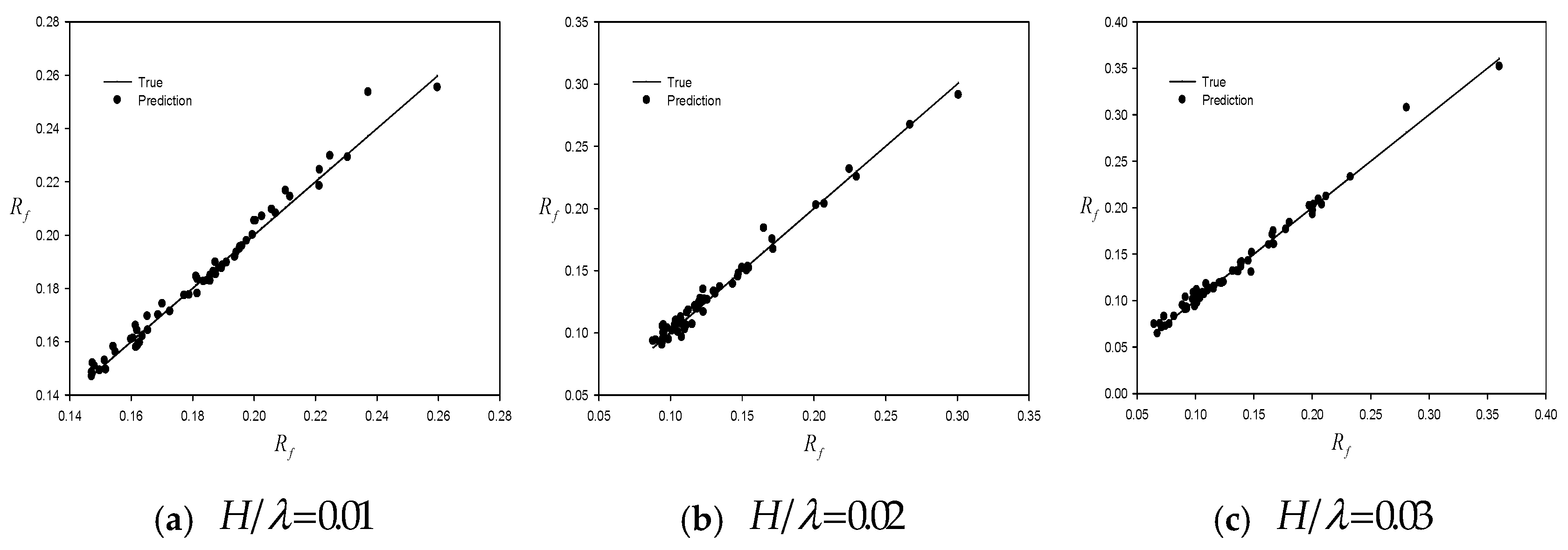
score close to 1.0 with the least MSE and MAE values indicates high prediction accuracy. Through a rigorous training process, the current ANN model achieved the highest scores. As previously mentioned, the performance of the trained ANN model is evaluated using the test data.
Table 2 presents the evaluation metrics for the output feature of the averaged reflection coefficient (
) for different wave steepness.
Figure 6 graphically displays the predicted values against the true values of the averaged reflection coefficient for different wave steepness. Predictions closer to the true values indicate a good prediction capability of the model.
4.5. Predictions Using a Larger Dataset
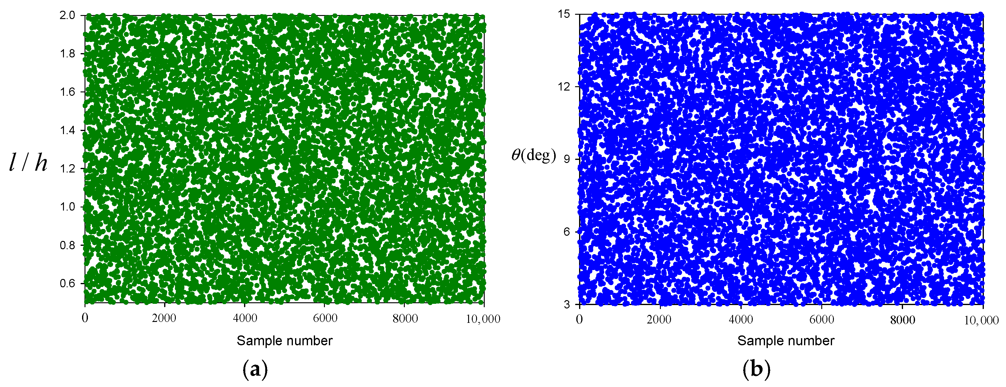
To determine the optimal design parameters, a larger set of possible combinations of design parameters needs to be considered in the analysis. Therefore, a larger dataset consisting of 10,000 samples was generated utilizing the Latin Hypercube Sampling (LHS) method. These samples are evenly distributed within the defined boundaries for each input feature, as shown in
Figure 7, providing a thorough representation of the design parameter combinations. Using these generated input datasets, the trained ANN model predicted the averaged reflection coefficient.
4.6. Weighted Sum Model (WSM)
The design parameters of non-dimensional plate length and inclined angle were optimized to minimize the averaged reflection coefficient (
) and the spatial footprint (
). The reflection coefficient was predicted using the trained ANN model outlined in the previous section, while the spatial footprint was calculated based on the plate length and the inclined angle, utilizing the larger dataset. To address the two objectives in the optimization process, a weighted sum model (WSM) was applied, and weighting factors were incorporated to represent their relative importance. The WSM is a well-known and simple multi-criteria decision-making approach used to evaluate multiple alternatives based on various decision criteria. Criteria are the attributes or factors taken into account during the decision-making process. This study has multiple criteria, such as the averaged reflection coefficient and the spatial footprint. Each criterion may carry a different level of importance or weight based on the context. Alternatives represent the various options or solutions available for evaluation, with each alternative assessed on how effectively it meets the criteria. The generated dataset of the reflection coefficient and the spatial footprint were utilized to prepare these alternatives. Weighting involves assigning relative importance to each criterion, representing its significance in the decision-making process. Scoring evaluates each alternative against each criterion, resulting in a numerical score that indicates how well the alternative fulfills the criterion. Finally, aggregation combines the scores and weights to yield an overall assessment of each alternative. The formula is given below:
where
is the overall score of the alternative
,
is the weighting factor for
,
is the weighting factor for
, and
and
are the normalized values of alternative
. The normalization is carried out using the MinMaxScaler as given in Equation (26). The weighting factor ratios (
) are assigned as
,
, and
, where the ratio
denotes the optimization is based solely on the reflection coefficient, the ratio
indicates that the reflection coefficient is significantly prioritized over the spatial footprint, and the ratio
means both are given nearly equal importance with a 20% preference for the reflection coefficient.
6. Discussion
From the top 10 optimal design parameters (
Table 3), it is observed that when the optimization is based only on the averaged reflection coefficient (
), minimal reflection is observed when the porous plate is comparatively long around
, with inclined angles of
for
. However, for
and
, the optimal non-dimensional plate length (
) is reduced to 1.49 and 1.76 with an optimal inclined angle of
and
, respectively. This optimal configuration based on (
) might minimize reflection but increase the spatial footprint that a wave absorber occupies. When the optimization significantly prioritizes the reflection coefficient over the spatial footprint (
), the optimal non-dimensional plate length (
) is substantially reduced to 1.16, with a slight decrease in the inclined angle to
for
. This change results in a slight increase in the reflection coefficient but a significant reduction in the spatial footprint. However, for
, the optimal non-dimensional plate length and inclined angle show insignificant change, resulting in minimal changes to both the reflection coefficient and the spatial footprint. For
, the optimal non-dimensional plate length and inclined angle decrease slightly, along with a reduction in the corresponding spatial footprint, while the reflection coefficient increases slightly. When the optimization is performed with a 20% preference for the reflection coefficient over the spatial footprint (
), the reduction in the optimal non-dimensional plate length and inclined angle is the same as in the previous weighting ratio for
. Whereas, for
and
, the optimal non-dimensional plate length (
) is substantially reduced to 0.52 and 0.58, with an increase in the inclined angle of
and
, respectively. This results in a greater increase in the reflection coefficient but a substantial reduction in the spatial footprint. Based on the observations, the optimal design parameters of weighting factor ratios (
) appear to be a more reasonable choice, effectively balancing the tradeoff between the reflection coefficient and the spatial footprint criteria. These results provide optimal design parameters based on the relative importance of the criteria, which will facilitate the decision-making process according to specific preferences.
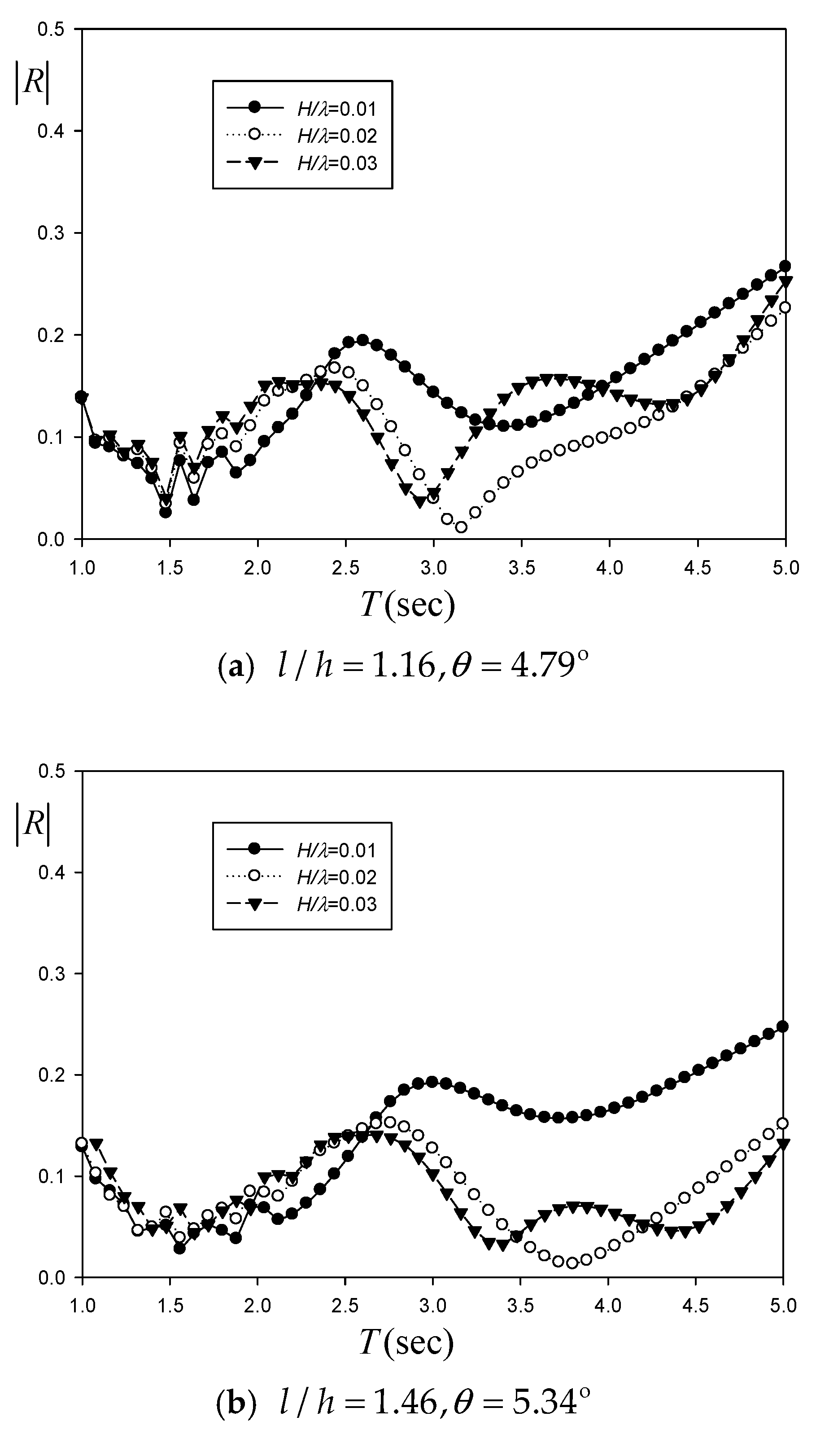
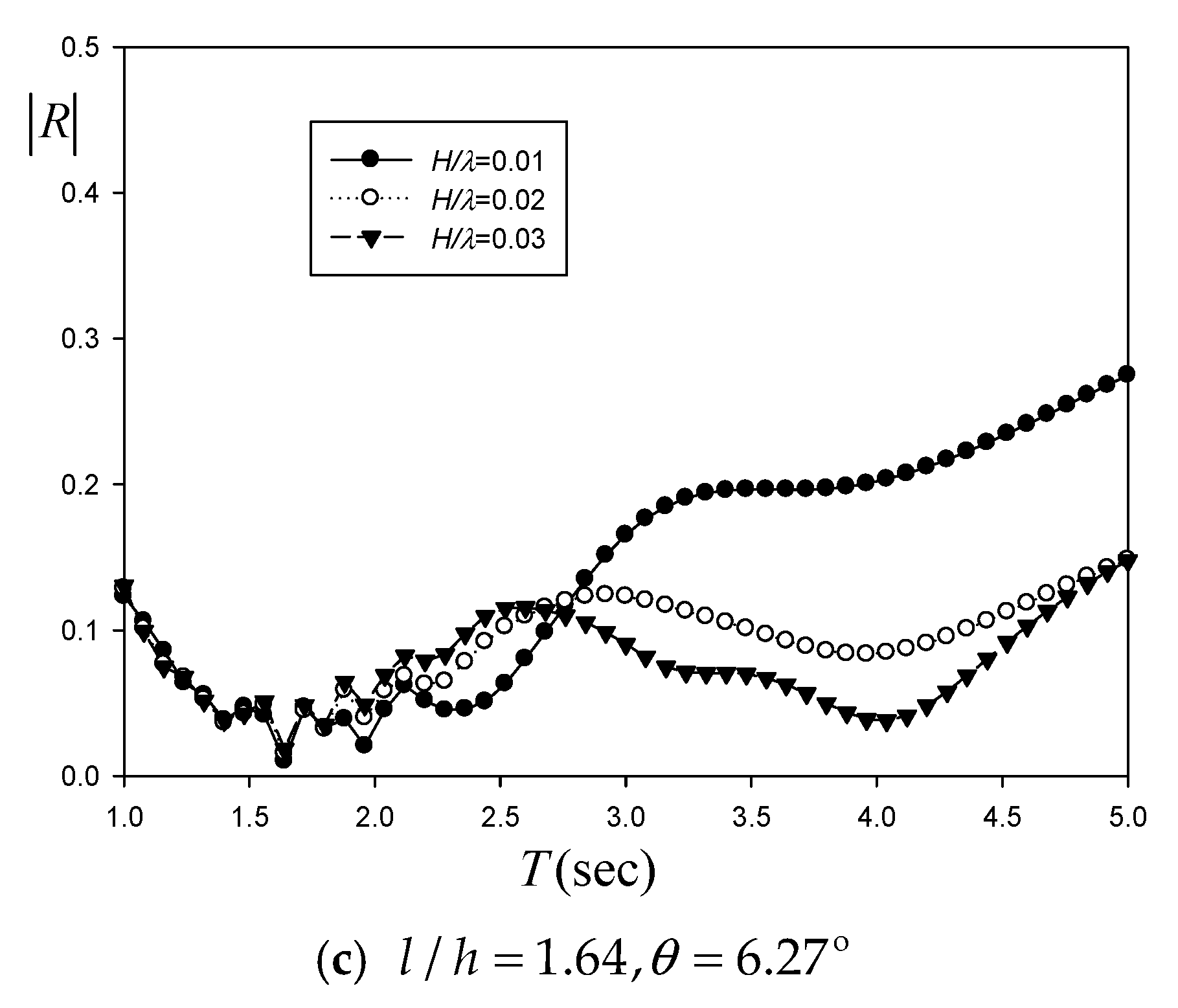
Based on
Figure 10, all reflection coefficients are maintained below 0.2 within the entire range of the wave period. The reflection coefficient of the steeper wave is lower, which implies that wave steepness (or nonlinearity) significantly influences overall performance. The averaged reflection coefficients across the wave period range of 1.0~5.0 s are 0.145, 0.109, and 0.128 in ascending order of wave steepness at
and
. With another optimal value of
and
, the averaged reflection coefficients are 0.139, 0.084, and 0.083 with increasing wave steepness. The final optimal design parameter of
and
gives the averaged reflection coefficients of 0.142, 0.091, and 0.078. Among the three options for optimal design parameters of the wave absorber,
and
seems to be the most effective solution.
7. Conclusions
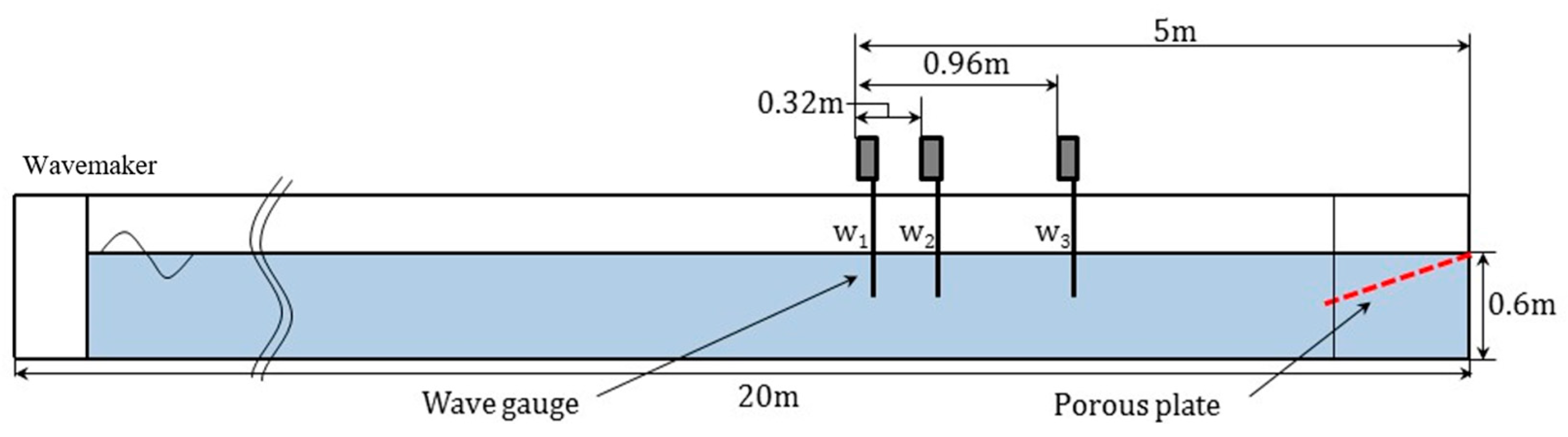
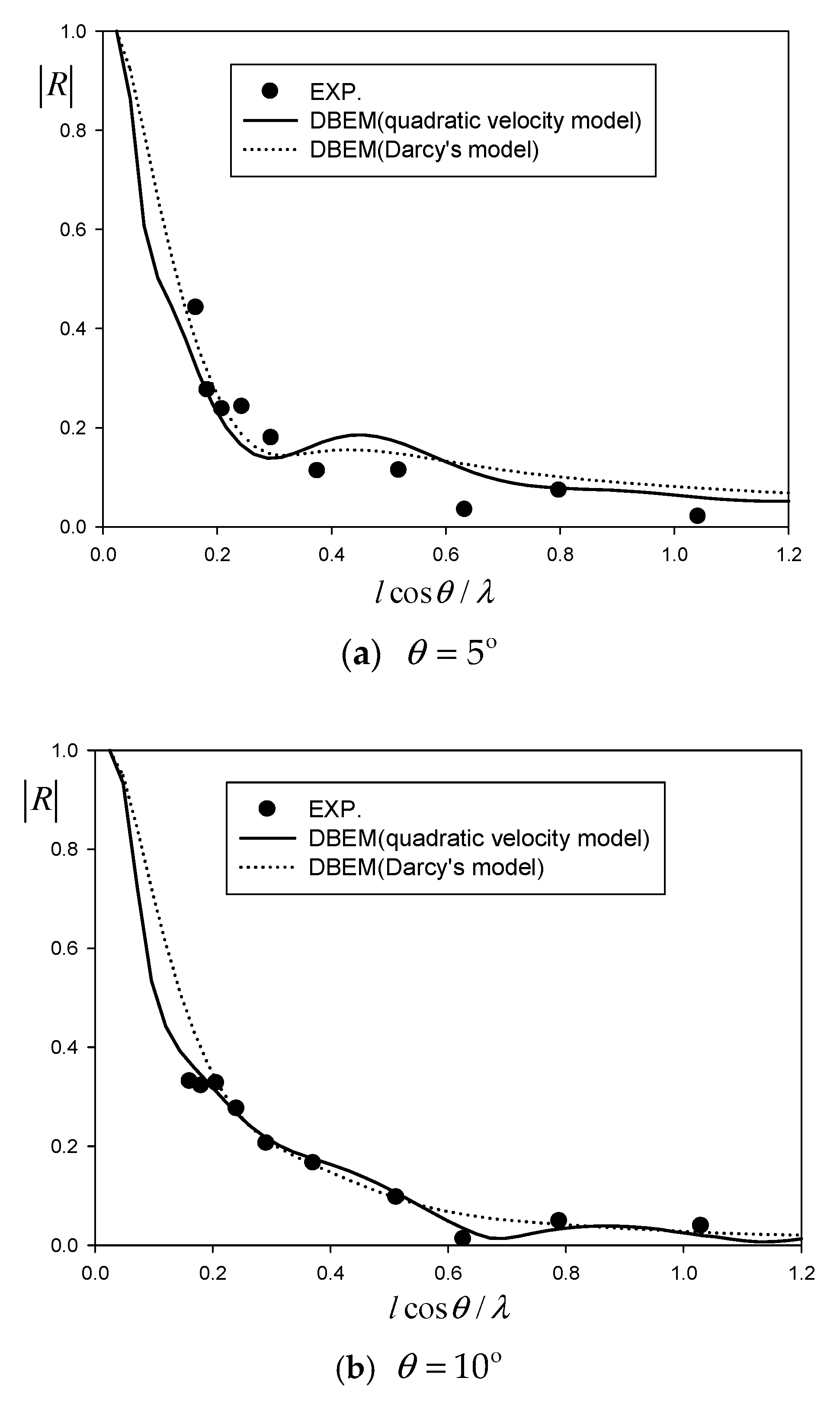
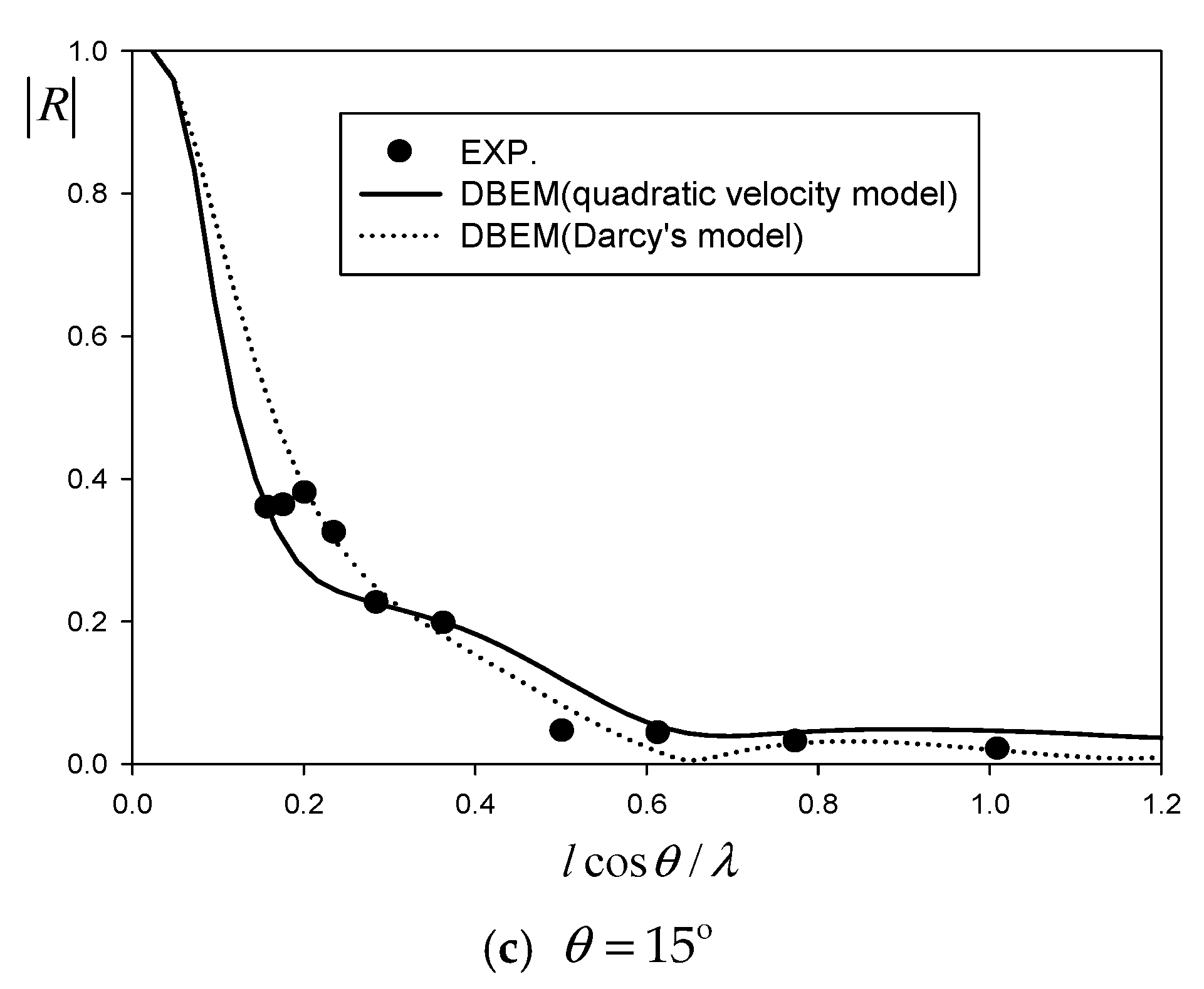
This study focuses on finding optimal design parameters for a wave absorber using an inclined porous plate, employing an artificial neural network (ANN) model to enhance the operating efficiency of a wave tank by minimizing both the averaged reflection coefficient () and the spatial footprint () of the porous plate. The dual boundary element method (DBEM) was employed as a numerical approach, combined with the quadratic velocity model and linear Darcy’s model, to account for energy dissipation through an inclined porous plate. The numerical results were validated through experiments conducted in a two-dimensional wave flume.
The design parameters influencing the reflection coefficient were chosen to be the inclination angle and the non-dimensional plate length, whereas the key parameter porosity was fixed at 0.1. The training dataset for the ANN model consists of random input features corresponding to these design parameters, along with an output feature of the averaged reflection coefficient, which is determined using the developed DBEM model. The ANN model was effectively trained by optimizing hyperparameters to maximize the score while minimizing both the mean squared error (MSE) and mean absolute error (MAE), leading to a model with high prediction accuracy. Then, the trained ANN model was utilized to make predictions of the averaged reflection coefficient with a larger random input feature dataset. The ANN model reduces the need for extensive numerical calculations while maintaining accuracy. In the optimization process focused on minimizing both wave reflection and spatial footprint, weighting factors were assigned according to their relative importance, utilizing the weighted sum model (WSM) within the multi-criteria decision-making approach. When the optimization is performed with a weighting factor () that significantly prioritizes minimizing reflection over the spatial footprint, the optimal design parameter with and seems to be a reasonable choice, effectively balancing both the objectives required in the design of a wave absorber. The ensemble of various methods provided a computationally efficient yet technically robust optimization with a multi-criteria framework that supports objective-driven design, facilitating informed decision making. While the machine learning approach shows great potential, a limited dataset may lead to an underestimation or overestimation of performance. Therefore, additional datasets and experimental studies are needed to validate these findings.


