Traffic Conflict Prediction for Sharp Turns on Mountain Roads Based on Driver Behavior Patterns

Abstract

This investigation analyses driving behaviors that lead to accidents on overly sharp mountain road curves in Nanjing Province, China. We collected information through field observations and driving simulations while analyzing key indicators like the mean speed of vehicles and spacing between vehicles. The FP-Growth algorithm was used to identify frequent behavioral patterns and measure their relationship with traffic conflicts. The findings showed that unsafe driver behavior on sharp turns was common, while the combination of “speeding–tailgating–frequent lane changing” behavior increased conflict risk by 3.7 times. A predictive LSTM neural network model was developed with driver, vehicle, road, and environmental factors. Testing on 4795 samples achieved 83.7% accuracy in foreseeing conflict risk levels. The model, which distinguishes between safety conditions and three severity levels of potential conflict, can provide the most fundamental level of safety needed. The research provides quantitative tools for improved road safety management aimed at supporting real evidence-based “safe roads” approaches.

1. Introduction

Mountainous roads are essential infrastructure for implementing the revitalization strategy, and they can help mountainous areas achieve high-quality development in terms of both economic and social benefits. Improving the construction of mountainous roads is of great significance in promoting industrial development and advancing urban–rural integration [1]. However, due to terrain, landform, and construction standards, traffic safety facilities on mountainous roads are generally underdeveloped. The road alignment is suboptimal, with complex and diverse traffic structures, sharp turns, and steep slopes [2,3] continuously increasing traffic accident rates. To effectively reduce the incidence of traffic accidents and improve road safety, it is necessary to predict traffic accidents at sharp turns on mountainous roads.

Previous research has established that unsafe driving behaviors significantly contribute to traffic conflicts on challenging road segments. Han et al. [4] identified key risk factors for professional truck drivers in China, including negligence and inappropriate driving times. Studies by Ji et al. [5] and Huliwei et al. [6] specifically examined mountain roads, developing risk prediction models based on traffic flows and dangerous driving behaviors. Branzi et al. [7] assessed overtaking maneuvers on rural two-lane roads, while other researchers [8,9] employed various methodologies—from driving simulators to vehicle sensors—to characterize driver behavior through parameters like speed, acceleration, and steering patterns. Ting et al. [10] defined dangerous following behavior based on parameters from the intelligent driver model, while Huiying et al. [11] developed a lane-change traffic conflict prediction model using the XGBoost algorithm. Zhigang et al. [12] demonstrated that traffic accidents in road tunnel clusters were primarily caused by poor driving behaviors, and Weihua et al. [13] used TTC and PET models as criteria for determining rear-end collisions and lane-change conflicts. These studies collectively demonstrate that behavioral combinations, rather than isolated actions, most significantly influence conflict probability.

Advancements in intelligent transportation systems have enabled the development of sophisticated predictive models. Researchers have employed various approaches, including the Extreme Value Theory (EVT) model [14], proxy and Bayesian mixed gamma-GPD models [15], and machine learning techniques. Nazir et al. [16] used a Bayesian non-stationary Generalized Extreme Value model to evaluate car-following crash risk, while Wu et al. [17] proposed a cycle-level traffic conflict prediction method using LiDAR data at signalized intersections. Lv et al. [18] used roadside fine perception data to generate SSMs as input for real-time collision prediction models, and Tao et al. [19] proposed a trajectory prediction method based on graph convolutional neural networks. Nan Z et al. [20] analyzed traffic conflict indicators based on the indirect safety assessment model, while Karri et al. [21] and Formosa et al. [22] investigated machine learning techniques for predicting traffic conflicts. These studies highlight the transition from post-event analysis to proactive prediction but demonstrate limited application in mountainous settings with their unique geometric and environmental challenges.

Recent studies have successfully applied data mining techniques to traffic safety analysis. The FP-Growth algorithm has demonstrated superior capability in identifying complex behavioral patterns leading to traffic incidents. Fang et al. [23] used the FP-Growth algorithm to analyze elderly pedestrian traffic accidents, while Chang et al. [24] applied it to analyze SSD error data. Simultaneously, Long Short-Term Memory (LSTM) neural networks have shown promise in trajectory prediction and conflict detection. Cao et al. [25] proposed a real-time vehicle trajectory prediction method using a multilayer LSTM model, Talebloo et al. [26] focused on detecting aggressive driving behavior using deep learning techniques, and Islam et al. [27] proposed an LSTM model for predicting traffic conflicts using connected vehicle data. These computational approaches offer advantages in processing complex, heterogeneous data typical of mountain road environments.

Despite these advances, significant research gaps exist regarding mountain road safety. First, most existing studies focus on urban or highway segments, with limited attention to mountain roads’ unique characteristics. Second, relationships between driving behavior patterns and traffic conflicts in mountain environments remain sparsely studied. Finally, predictive models specifically calibrated for these challenging environments are largely absent. This study addresses these gaps by combining driving simulation experiments with field observations to capture driver behavior and conflicts at sharp turns in mountain regions, employing the FP-Growth method [28,29,30] to identify behavioral associations with conflicts, and developing an LSTM-based prediction model [31,32,33] for mountain road safety management.

2. Materials and Methods

This study focuses on a challenging road segment of the X412 County Road located in Nanjing Province, China. Through comprehensive data collection and systematic processing procedures, this study establishes a robust foundation for analyzing traffic patterns and safety implications along this geometrically complex road section, ultimately supporting evidence-based decision-making for safety improvements.

The research framework is shown in Figure 1. The first part is data acquisition and data preprocessing; the second part is analysis of driving behavior characteristics; the third part is the derivation of FP-Growth mining association rules from composite transaction data; the fourth part is the construction of a traffic conflict prediction model.

2.1. Data Collection Environment and Procedures

2.1.1. Selection of Data Collection Environment

For analyzing the correlation between driving behavior and traffic conflicts, this study examines a segment of the X412 County Road in Nanjing Province, China, extending 8.2 km from Lishu Village to Damao Village (as shown in Figure 2). This segment, typical of mountain roads in China, features a design speed of 40 km/h and incorporates a two-lane configuration with 3.5 m lane widths. The road geometry presents particularly challenging characteristics, with only four sections exhibiting horizontal curve radii exceeding 100 m, comprising less than 30% of the total length. The alignment includes 12 sharp turns, defined as curves with vertex angles greater than 90 degrees and radii less than 60 m, many of which qualify as hairpin bends. These sharp turns frequently coincide with steep gradients, characterized by longitudinal slopes averaging 5.3% and reaching maximums of 8%, which differs notably from mountain roads in European countries, where slopes can reach 12% with horizontal curves with 30 m radii. The section’s significance is amplified by its role as a crucial transportation link, experiencing substantial traffic volumes with a diverse vehicle composition, including a considerable proportion of heavy vehicles. The combination of challenging geometric features, significant traffic demands, and complex vehicle interactions makes this segment particularly suitable for studying driving behavior and traffic conflicts. The road’s characteristics, while representative of Chinese mountain roads, create unique safety challenges that warrant detailed investigation, especially considering the frequency of sharp turns and their correlation with accident risks.

The road segment, classified as a secondary road according to Chinese road design standards, presents significant geometric complexity with sharp turns and steep slopes. The roadway infrastructure follows standard design specifications with a designated speed of 40 km/h and comprises a two-lane configuration, each lane measuring 3.5 m in width, complemented by 1.5 m shoulders on both sides. The geometric design incorporates horizontal curves with minimum radii of 60 m, accommodating the mountainous terrain while maintaining safety standards. The vertical alignment exhibits considerable variation, with longitudinal grades reaching up to 8% and cross slopes maintained at 4% for adequate drainage. The clear width of 8.5 m and Road Grade-II loading capacity ensure sufficient space for vehicle movement and structural integrity. These geometric characteristics, while challenging from an operational perspective, are consistent with the regional topography and local transportation needs.

2.1.2. Driving Behavior Data Collection

To obtain the behavioral data of drivers on sharp turns, a driving simulation test was conducted using the driving simulator developed by Beihang University. Firstly, based on the measured road profile data of the X412 County Road test section, a virtual road scene model with the same height as the actual road section was built in the driving simulator, and parameters such as traffic flow, weather, and vehicle conditions matching the actual conditions were set. Then, 30 drivers were recruited as participants for the experiment, covering different genders, ages, and levels of driving experience to ensure representativeness and diversity of samples. During the experiment process, each driver had to complete two simulated driving tasks from Damao Village to Lishu Village with a time interval of no less than 7 days to eliminate the impact of learning effects. The drivers wore SMI eye-tracking glasses to record their visual attention behavior data. The driving simulator was equipped with a steering wheel, a pedal-force feedback device, and a multi-channel data acquisition system to collect the drivers’ speed, acceleration, manipulation amount, and other driving behavior data at a sampling frequency of 60 Hz. Through high-fidelity road scene reproduction and detailed collection of driving behavior data, rich behavioral data samples of drivers on sharp turns were obtained, laying the foundation for subsequent analysis. The instruments used in this experiment are shown in Figure 3.

2.1.3. Extraction of Traffic Conflict Data

To obtain traffic conflict data for the experimental section, six observation points were established along the X412 County Road from Lishu Village to Damao Village, encompassing diverse road geometries, including sharp curve sections (radii < 60 m), gentle curve sections (radii between 60 m and 100 m), slope sections, and tunnel sections. Each observation point was staffed with two professional observers and equipped with a high-definition camera (SONY AX700, Tokyo, Japan). The study conducted continuous observations over three months, maintaining daily 12 h observation periods (8:00–20:00), accumulating 2000 h of total observation time. All observations strictly adhered to the international standard for Traffic Conflict Technique (TICT) [34], documenting comprehensive data, including vehicle conflict time, location, type, and severity level, while maintaining video recordings of key areas and high-risk events. Through the integration of manual records and video analysis methods, the study collected detailed traffic conflict data encompassing 960 valid conflict events, including rear-end collisions, head-on conflicts, and lane-changing conflicts, with severity levels ranging from minor to major. The extensive database of traffic conflicts, categorized by both type and severity, provides a robust foundation for analyzing the correlation between driving behavior and traffic conflicts in this academic research investigation.

2.1.4. Data Matching and Preprocessing

To effectively integrate driving behavior data with traffic conflict data, a set of data-matching and preprocessing programs was developed. Firstly, the driving simulation test data and traffic conflict observation data were synchronized according to the time series, and the driving behavior sequence data 30 s before and after the occurrence of a conflict event were extracted to form matched pairs of driving behavior–traffic conflict data. Subsequently, the matched data were subjected to noise reduction [35,36] and outlier handling [37,38] to eliminate invalid or abnormal data caused by equipment malfunctions, signal loss, etc., ensuring the quality of the data. Then, statistical features were extracted from valid matched data, including mean speed, speed standard deviation, mean acceleration, acceleration standard deviation, and minimum headway distance as driving behavior indicators, as well as types and severity levels of traffic conflicts as safety indicators. Finally, the extracted driving behavior features and safety indicators were stored and labeled in a consistent format to create structured datasets for correlation analysis and predictive model construction. Through systematic data matching and preprocessing processes, we achieved effective integration of cross-domain datasets, laying a solid foundation for further exploration of underlying patterns in driving behavior and traffic conflicts based on high-quality datasets.

2.1.5. Preparation of the Dataset

Based on the measured data, the training set, verification set, and test set were constructed. The data collection process was as follows:

(1) Data source: Data were collected from the typical sections of two mountain roads, the X412 County Road and the X001 County Road.

(2) Data collection time: six consecutive months (March to August 2022).

(3) Data types:

Vehicle sensor data: speed, acceleration, steering wheel angle, etc.

Meteorological environment data: visibility, precipitation, wind speed, etc.

Driver information: age, driving experience, etc.

(4) Sampling frequency: vehicle data (10 Hz), environmental data (1 min/time).

The 47,952 samples were classified into four categories: safety, minor conflict, general conflict, and serious conflict. The datasets were divided as shown in

Table 1. Dataset partitioning.

Dataset	Conflict Sample	Normal Sample	Total	Ratio
Training Set	3886	34,476	38,362	80%
Validation Set	485	4310	4795	10%
Test Set	486	4309	4795	10%
Total	4857	43,095	47,952	100%

.

2.2. Methodological Framework

The FP-Growth algorithm was applied to discover frequent behavioral patterns and assess their relationship with traffic conflicts. A predictive LSTM neural network model was created using driver, vehicle, road, and environmental factors.

2.2.1. Principle of the FP-Growth Algorithm

Understanding the links between driving practices and traffic disruptions is fundamental for automating safety measures for mountainous road usage. Pattern recognition, such as associational rule mining, offers a systematic method to uncover associated driving behaviors that may contribute to accidents. In the context of collision prediction analysis that employs behavioral pattern mining, we chose the FP-Growth algorithm as it is best known for its speed when processing complicated behavioral data. Traditional methods of rule mining, such as Apriori, often lead to computation overload due to multiple passes through their databases, along with the formation of expansive candidate sets. In our case, where we were dealing with over forty-seven thousand sequences of driving behavior intentions and conflicts, FP-Growth allowed for quicker processing times because it builds a condensed tree structure that does not lose materials for analysis—this is useful in keeping analytical strength when dealing with enormous amounts of data. Studies conducted before were proposed by Li. FP-Growth has been shown to combine the riskiest driving behaviors in urban settings, but it does apply to mountainous road contexts [39], which clearly outlines how FP-Growth has shown great value in combining the riskiest behaviors in urban driving environments. In urban road environments, there are possibilities of switching from reactive measures to strategies that preemptively mitigate collisions. FP-Growth has demonstrated its ability to combine the riskiest driving behaviors in urban road environments, though limited applications exist in mountainous context roads. By pulling out behavior driving patterns that are significantly related to accident conflict types, this approach enables efforts to (1) measure and identify the most dangerous behavioral combinations, (2) quantify their relative risk levels, and (3) take a proactive approach to getting rid of the causes instead of the effects of accidents [40,41].

An FP-Tree (Frequent Pattern Tree) is a compact data structure used to construct and analyze driving behavior data and to discover frequent patterns within them. The FP-Growth algorithm employs frequent growth techniques to analyze data patterns within driving behavior. In this context of traffic safety analysis, driving behaviors such as speeding, short following distance, and lane changing, which co-occur in certain driving situations that result in conflicts, can be systematically analyzed with the use of the FP-Tree algorithm. For our analysis of drivers’ behaviors, the algorithm follows the procedure below:

Initial Data Scan: The algorithm scans the driving behavior–traffic conflict dataset and looks for certain behaviors that appear frequently enough to be considered valid (exceed the minimum support threshold). If such behaviors are valid, they are ordered by their support counts within a frequent item header list. For example, “speeding” (TS↑) in our dataset had an occurrence rate of 85% and “short headway” (LK↓) had a frequency of 72%.

FP-Tree Construction: The algorithm adds every driving behavior sequence separately into the FP-Tree as it builds the FP-Tree, which results in the creation of a dataset representation via compression of common prefixes. In our implementation, paths in the tree correspond to the sequence of driving behaviors that take place prior to a certain traffic conflict. An illustration of this construction process is demonstrated in Figure 4.

Pattern Mining: As noted earlier, once the FP-Tree is built, the algorithm uses a geometric approach to retrieve patterns. Starting from the least frequent behavior, it proceeds in reverse order to determine which combinations of behaviors are common. For every behavior, a conditional pattern base is extracted, and an FP-Tree is built. The tree is recursively mined for all frequent patterns until no more significant patterns are found.

This makes it easier to determine which combinations of driving behaviors are most closely associated with different types of traffic conflicts on mountain roads, thus enabling safety measures to be put in place.

2.2.2. LSTM Neural Network Structure Design

The formation of traffic conflict is a complex, dynamic process, and a prediction model should be able to describe the non-linear relationship between variables and consider the time-series effect. A Long Short-Term Memory network (LSTM) was chosen as the basic model architecture. An LSTM network is an improved recurrent neural network, which can effectively learn and retain long-term dependent information by introducing gated units and memory units, and it performs well in time-series prediction tasks. Figure 5 shows the structure of the constructed LSTM traffic conflict prediction model. The model takes the characteristic variables of the past n time steps as input and outputs the traffic conflict risk level of the future 1 time step. The model mainly includes the following parts:

(1) Input layer: Receives the time series composed of 11 dimensional characteristic variables; the length of the series is n, that is, where $\mathrm{X}=\left({\mathrm{x}}_1,{\mathrm{x}}_2,\cdots ,{\mathrm{x}}_{\mathrm{n}}\right),{ \mathrm{x}}_{\mathrm{t}}\in {\mathrm{R}}^{11}$.

(2) LSTM layer: Contains m LSTM units, which are used to extract the timing features of the input sequence. Each LSTM unit receives the input of the current moment, $x_t$; the hidden state, $h_{t-1}$; and the memory state of the previous moment, $c_{t-1}$, and comprehensively updates the hidden state, $h_t$, and the state of the current moment, $c_t$.

$$\begin{array}{cc}{\mathit{i}}_t& =\mathit{\sigma }({\mathit{W}}_{ii}{\mathit{x}}_t+{\mathit{W}}_{hi}{\mathit{h}}_{t-1}+{\mathit{b}}_i)\\ {\mathit{f}}_t& =\mathit{\sigma }({\mathit{W}}_{if}{\mathit{x}}_t+{\mathit{W}}_{hf}{\mathit{h}}_{t-1}+{\mathit{b}}_f)\\ {\mathit{o}}_t& =\mathit{\sigma }({\mathit{W}}_{io}{\mathit{x}}_t+{\mathit{W}}_{ho}{\mathit{h}}_{t-1}+{\mathit{b}}_o)\\ {\tilde{\mathit{c}}}_t& =\tanh ({\mathit{W}}_{ic}{\mathit{x}}_t+{\mathit{W}}_{hc}{\mathit{h}}_{t-1}+{\mathit{b}}_c)\\ {\mathit{c}}_t& ={\mathit{f}}_t\odot {\mathit{c}}_{t-1}+{\mathit{i}}_t\odot {\tilde{\mathit{c}}}_t\\ {\mathit{h}}_t& ={\mathit{o}}_t\odot \tanh ({\mathit{c}}_t)\end{array}$$

where $i_t$, $f_t$, and $o_t$ represent the input gate, forget gate, and output gate, respectively. $\odot$ denotes element-wise multiplication, while $\mathrm{\sigma }(·)$ stands for the Sigmoid activation function.

Fully connected layer: Passes the output, $h_n$, of the LSTM layer to a fully connected layer and uses the Softmax function to map it onto a probability distribution of traffic conflict risk levels.

$$y=\mathrm{softmax}(Why{h}_n+b_y)$$

(1)

where $\mathrm{y}\in {\mathrm{R}}^{\mathrm{k}}$ and k is the number of categories of traffic conflict risk levels.

Output layer: Based on the probability distribution of y, the predicted level of traffic conflict risk is the output.

$$\widehat{y}={\mathrm{argmax}}_i{y}_i$$

(2)

By using the memory ability of the LSTM unit, the model can adaptively learn the long-term dependence pattern in the evolution process of traffic conflict and provide timely warning of the conflict risk level in the future period according to the current driving behavior, road condition environment, and other factors to provide decision support for drivers and traffic management departments.

Figure 5. Structure of LSTM unit.

Figure 5. Structure of LSTM unit.

2.3. Prediction Model Design

2.3.1. Model Variable Selection

The first step in constructing a traffic conflict prediction model is to select appropriate input variables. Based on the above association rules, 11 key variables are selected as model inputs from the aspects of driving behavior, vehicle state, road condition environment, etc., as shown in

Table 2. Input variables of traffic conflict prediction model.

Categories	Variable Names	Symbol	Units	Data Sources
Driving behavior	Average speed	AS	km/h	On-board sensors
	Standard deviation of speed	SSD	km/h	Vehicle sensor
	Average time headway	AH	s	In-car sensors
	Standard deviation of headway	HSD	s	In-car sensors
	Average lateral acceleration	ALA	m/s2	In-vehicle sensors
Road condition environment	Road curvature	RC	1/m	Road alignment measurement
	Coefficient of road adhesion	RAC	Dimensionless	Pavement condition monitoring
	Road grade	RG	%	Road alignment measurement
	Visibility	V	m	Posted by Weather Department
	Wind Speed	WS	m/s	Issued by the Weather Department
Driver	Driver age	DA	years	Driver information registration

. In addition, considering that traffic conflict is related to individual factors such as a driver’s reaction time and psychological state, the demographic variable of driver’s age (DA) is included. Figure 6 shows the distribution characteristics of various variables. By comprehensively considering multiple influencing factors, such as person–vehicle–road–environment, internal and external causes of traffic conflicts can be described, laying a more comprehensive and reliable data foundation for the construction of the prediction model.

2.3.2. Model Parameter Settings

The LSTM prediction model is implemented using the PyTorch 1.12.1 deep learning framework. The main hyperparameter settings are as follows:

(1) LSTM layer:

Number of hidden layer neurons: 128.

Number of layers: 2.

Enter the time step: 30.

(2) Full connection layer:

Number of neurons: 64.

(3) Output layer:

Number of neurons: 4 (corresponding to four conflict levels).

(4) Batch size: 64.

(5) Learning rate: 0.001.

(6) Optimization algorithm: Adam.

(7) Loss function: cross-entropy.

(8) Early Stop method Patience: 10 epochs.

To illustrate the parameter selection process, Figure 7 shows the learning rate vs. model performance validation accuracy graph.

A small-batch gradient descent method is adopted for model training, parameters are iteratively updated on the training set, and performance is evaluated on the verification set. The training process is as follows:

(1) Data loading: Using PyTorch’s DataLoader, set batch_size = 64, shuffle = True.

(2) Forward propagation: Input 30 s of sequence data to obtain predictive output.

(3) Back propagation: Calculate the loss and update the model parameters.

(4) Validation: Evaluate the model on the validation set after each epoch.

To visualize the training process, record the training loss, training accuracy, validation loss, and validation accuracy for each epoch (as shown in Figure 8).

As can be seen from the figure, the performance of the model on both the training set and the verification set improves with the increase in the number of epochs. Training losses and validation losses continue to decline, while accuracy continues to rise. Validation set performance is optimal at about Epoch 42, when the validation set accuracy is 85.6% and the loss is 0.38.

To prevent overfitting, the early stop method is applied. When the verification set performance has not improved for 10 consecutive epochs, the training process is automatically stopped. In the experiment, after the model reached the best performance at the 42nd Epoch, it was trained for another 10 epochs without further improvement in performance, so the training stopped at the 52nd Epoch. As shown in the Figure 9. It should stop before the dark blue dashed line.

In this way, the training is stopped in time when the model reaches the best performance, and the overfitting problem is avoided.

3. Results

3.1. Driving Behavior Characteristics Analysis Results

Based on the collected and processed data, we can identify key features in driving behavior. Specifically, we selected speed, acceleration, headway distance, and steering as the driving behavior characteristics to evaluate the safety and efficiency of drivers.

3.1.1. Speed Characteristics

Speed is an important indicator to characterize driving behavior. We examined speed choice patterns at sharp turns based on data from 30 drivers who took part in our driving simulation exercises and cumulatively made 60 drives (each driver undertook two trials) on the virtual stretch of road X412. This yielded 18,540 speed measurements at various points along the simulated route. Statistical indicators of speed in different sections are shown in

Table 3. Speed statistics of different sections.

Index (km/h)	Straight-Line Section	Curved Section
Mean	63.5	48.2
Standard deviation	8.6	12.4
85% quantile value	72.1	60.6

. The results show that the speed of the driver in the curve section is significantly lower than that in the adjacent straight section, but still more than 30% of the drivers have different degrees of speeding behavior. By analyzing the correlation between the driver’s speed selection and the curve geometry index, it can be seen that when the curve radius is less than 60 m, the driver’s 85% fractional speed decreases significantly with the decrease in the curve radius, and the decline rate is higher than the road’s design speed, indicating that it is difficult for the driver to control the speed reasonably according to the linear conditions. Based on the speed–curve radius data, a prediction model of 85% percentile speed was constructed:

$$V_{85}=61.72+0.41R-17.35/R$$

(3)

where V₈₅ represents the 85th percentile speed (km/h) and R stands for the radius of the curve (m). Experimental verification confirmed that this model can be used for predicting speeds and evaluating safety on sharp turns.

3.1.2. Acceleration Characteristics

Acceleration features are linked to both the behavioral adaptability of a driver’s speed change and their driving style. The acceleration statistical indicators of different sections are shown in

Table 4. Statistical indicators of acceleration in different sections.

Index (m/s2)	Straight-Line Section	Curved Section
Mean longitudinal acceleration	0.35	1.12
Longitudinal acceleration standard deviation	0.42	0.86
Mean lateral acceleration	0.28	1.50
Lateral acceleration standard deviation	0.37	1.15

. We looked into both longitudinal (speed changes) and lateral (turning) accelerations from the simulation data, which encompassed 22,620 measurements of acceleration.

$$J=\sqrt{{\displaystyle \frac{1}{T}}{\displaystyle {\int }_0^T((}{\displaystyle \frac{d{a}_x}{dt}}{)}^2+{({\displaystyle \frac{d{a}_y}{dt}})}^2)dt}$$

(4)

In the equation, J represents the rate of acceleration change (m/s³), where $a_x$ and $a_y$ denote the longitudinal and lateral accelerations (m/s²), respectively, and T stands for the time taken to pass through a sharp bend (s). A larger rate of acceleration change indicates more frequent and abrupt driver control.

$$DR=3.27-1.08\ln R+0.82J$$

(5)

where DR represents the level of driving risk (1–5, with higher values indicating greater risk), R stands for the radius of the curve (m), and J denotes the rate of acceleration change (m/s³). Experimental verification has shown that this model can be used for the quantitative assessment of driving risk on sharp turns.

3.1.3. Front Time Feature

The amount of time given as a headway is an essential parameter for the analysis of the safety of the following behavior of drivers. The researcher analyzed 14,760 simulated headway time measurements, and video analysis techniques were applied to 2340 field observation measurements. The driving simulation data were analyzed, and the statistical results of the headway time characteristics of drivers in the sharp-curve sections are shown in

Table 5. Statistical indicators of time headway in different segments.

Index	Unit	Straight Section	Curved Section
Average headway	s	2.15	1.38
Standard deviation of headway	s	0.92	0.75
Minimum front time	s	0.85	0.47
Hazardous headway ratio *	%	12	28

* Note: Hazardous headway ratio refers to the percentage of time headways are less than 1.0 s.

. The results indicate that the average headway time in curved sections is significantly smaller than that in straight sections, and more than 25% of drivers have a dangerous headway time of less than 1 s, reflecting a higher risk of rear-end collisions. A safety headway time model based on vehicle speed and reaction time was constructed:

$$TH{W}_s={\displaystyle \frac{V_f}{3.6}}{T}_r+{\displaystyle \frac{V_f^2-V_l^2}{25.92(a_f-a_g)}}$$

(6)

where THW_s is the safe headway (s); V_f and V_l are the speeds of the front and rear vehicles, respectively (km/h); and T_r is the driver’s reaction time (1.5 s), which represent the accelerations of the front and rear vehicles respectively (m/s²). The model comprehensively considers the influence of speed difference and reaction time on the following safety.

$$THR={\displaystyle \frac{TH{W}_s-TH{W}_a}{TH{W}_s}}$$

(7)

where $TH{W}_a$ is the actual time headway (s). The larger the THR, the more the actual time headway deviates from the safety threshold and the higher the risk of a rear-end collision.

3.1.4. Steering Characteristics

The ability of drivers to adjust to curve features and their accuracy in path tracking is indicated by the steering characteristics. We studied the 19,860 dissections of the simulation data while concentrating on the steering wheel angle and the turn-on angle or steering rate. The characteristics of the steering wheel angle and the steering rate of drivers on sharp turns were analyzed, and the steering control index is shown in

Table 6. Steering control indicators of different sections.

Index (deg)	Straight-Line Section	Curved Section
Average steering angle	2.5	28.6
Deviation of the steering angle	1.2	12.4
Average steering speed	1.8	15.2
Steering-rate standard deviation	0.9	8.7

, indicating that the average steering angle and steering rate of drivers in curve sections are significantly higher than those in straight sections, and the degree of dispersion of steering actions is also significantly increased, reflecting more frequent and intense steering behaviors. The steering risk index was constructed to characterize the stability of steering behavior:

$$SRI={\displaystyle \frac{{\sigma }_{\delta }}{R}}$$

(8)

where SRI is the steering risk index (deg/m), ${\sigma }_{\delta }$ is the standard deviation of the steering angle (deg), and R is the radius of the bend (m). The greater the steering risk index, the more unstable the steering action of the driver and the lower the path-tracking accuracy. Based on the steering risk index, a steering ability evaluation model was proposed:

$$SC=e^{-0.24SRI}$$

(9)

where SC is the steering ability score (0–1); the higher the score, the stronger the steering ability of the driver. This model can be used to evaluate the driver’s ability to adapt to different cornering alignments.

3.1.5. Cluster Analysis of Driving Behavior

To understand driving behavior patterns identified during sharp turns, we carried out cluster analyses based on the characteristic indicators derived from our driving simulation experiments. For this analysis, we included data from all 30 participants who drove through 12 sharp turns on a simulated X412 road section, resulting in 360 driver–curve pairs. The dataset from the simulation was approached with K-means clustering to determine the four measurements of behavior: average speed through the curves, average acceleration, average time headway, and average steering wheel angle. We used the elbow method to find the optimal number of clusters and compute the within-cluster sum of squares over several clusters that were predetermined. The analysis suggested that four clusters would give a reasonable level of complexity to the model while providing sufficient explanatory power. To determine different driving styles at sharp turns, we performed cluster analysis on the characteristic indicators of speed, acceleration, headway, and steering angle of all drivers over all sharp turns, which resulted in 360 driver–curve pairs. The optimal cluster number of four was achieved through the elbow method, which determines the relative value of several clusters by the variance explained. The K-means algorithm was employed to determine the optimal number of clusters as four using the elbow method. Drivers were categorized into four classes, as shown in

Table 7. Clustering results of driving behavior.

Index	Category 1	Category 2	Category 3	Category 4
Average speed (km/h)	45.2	67.8	58.4	52.6
Average acceleration (m/s2)	0.68	1.52	1.85	0.73
Average headway (s)	2.25	1.12	0.96	2.68
Average steering Angle (deg)	18.6	32.5	38.2	15.4
Driver ratio (%)	28	22	18	32

. The first class exhibits a cautious and steady driving style with low speed, moderate acceleration, and steering amplitude. The second class demonstrates an aggressive and adventurous driving style with high speed and frequent steering and acceleration actions. The third class reflects a rough and reckless driving style with moderate speed but intense steering and acceleration, along with short headway distance. The fourth class displays a careful yet sluggish driving style with relatively stable speed and acceleration but delayed steering actions and long headway distance. Based on the clustering results, a comparison of accident risks for different driving patterns was conducted to construct an accident risk prediction model:

$$P_a={\displaystyle \frac{e^{-3.27+0.68v+1.12a+0.84\delta -0.52THW}}{1+e^{-3.27+0.68v+1.12a+0.84\delta -0.52THW}}}$$

(10)

where $p_a$ is the probability of an accident, v is the speed factor (0–5), a is the acceleration factor (0–5), $\delta$ is the steering factor (0–5), and THW is the headway factor (0–5).

Levels of driving risk, referenced in this analysis, were derived from a composite evaluation model based on the following four components: (1) measurements of deviation from internationally established standards and safety thresholds found in the scholarly literature, including those for safe curve navigation speeds and acceleration limits; (2) expert assessments conducted by three traffic safety engineers who independently evaluated 120 video recordings of driving behaviors at sharp turns, rating each on a defined risk scale; (3) correlation with actual traffic conflict outcomes recorded during our field observations; and (4) statistical analysis using Z-score calculations to quantify how each observed behavior deviated from established norms. For the risk assessment scale of 1 to 5, values were assigned using a weighted scoring technique based on the severity of overspeeding (25%), headway safety margin (25%), steering instability (20%), acceleration volatility (20%), and environmental variables (10%). This approach is likely to have fulfilled the criterion of our concern, which was to ensure that objective safety measures and real-world results accurately represented the value of risk levels.

In Table 7, the clustering results are outlined by displaying the centroid values associated with each behavioral variable for the four driver categories. These clusters correspond to different driving styles with varying levels of associated risk:

• Category 1: Cautious and Steady Drivers (28% of the sample)

This group has the lowest average speed of 45.2 km/h and moderate acceleration of 1.68 m/s², with a steering angle of 18.6 degrees. They also have the second-longest headway time of 2.25 s, which is above the safety threshold of 1.0 s. Instead of speed, these drivers prioritize safety and make sharp turns, having full control over their vehicles.

• Category 2: Aggressive and Adventurous Drivers (22% of the sample)

These drivers can maintain the highest speed while making turns at 67.8 km/h, which is far greater than the design speed of 40 km/h. They also exhibit a high acceleration of 1.52 m/s², with a headway time of 1.12 s, which is dangerously close to the critical safety threshold. This combination indicates vigorous behavior with very few safety limits.

• Category 3: Rough and Reckless Drivers (18% of the sample)

Within this category, while the average speed was not the highest recorded (58.4 km/h), the participants exhibited the most erratic control activity, which was highlighted by the highest recorded acceleration values (1.85 m/s²) and average steering angles (38.2 degrees). Alarmingly, they have the quickest headway time (0.96 s), which is below the safety threshold of 1.0 s. These drivers lack proper foresight and do not seem to adjust adequately to the anticipated road conditions.

• Category 4: Careful but Sluggish Drivers (32% of the sample)

Of all the categories, this is the most populous group. They retain average speeds of 52.6 km/h while keeping their rate of acceleration extremely low (0.73 m/s²) along with equally low average steering angles (15.4 degrees). They also keep exceedingly large headway distances (2.68 s), far surpassing what is necessary for safety. The behavior displayed suggests that there is a great amount of caution, which could be attributed to a lack of confidence or ability.

3.2. Association Rule Mining Results

3.2.1. Association Rule Generation

Focusing on the driving behavior patterns derived from the FP-Tree analysis, we developed association rules that estimate the relationship between certain driving behaviors and traffic conflicts. These rules are characterized as “if behavior pattern X occurs, then traffic conflict Y follows with probability Z”. The reliability and strength of these relations were managed through two parameters:

Minimum support threshold (min_sup = 0.02): This parameter specifies the minimum rate of occurrence of association between the behavior and conflict that qualifies as significant. We chose a very low baseline (0.02 or 2%) due to a preliminary data review that indicated that serious conflicts are infrequent occurrences. This value captures critical patterns that lead to immense conflicts while maintaining statistical significance. In comparison, prior research conducted in city settings (Zhang et al., 2022) [13] had an average range of 0.05–0.10, which, in turn, would have disregarded numerous important mountain-specific patterns in our model. Minimum confidence threshold (min_conf = 0.6): This parameter defines the minimum conditional probability required for a valid association rule. Our selection of 0.6 (60%) means that for a rule to be accepted, when the specified driving behavior pattern occurs, the associated traffic conflict must follow at least 60% of the time. This threshold was determined through cross-validation testing, which showed that lower values (0.4–0.5) produced too many spurious associations, while higher values (0.7–0.8) missed important moderate-strength relationships that were nonetheless actionable for safety interventions.

3.2.2. Algorithm Implementation Steps

Data coding: First, the traffic conflict data are encoded to extract the type and severity of the conflict:

(Rear-End, RE): {RE-Min, RE-Mod, RE-Sev}

(Lane-change, LC): {LC-Min, LC-Mod, LC-Sev}

(Cross, CR): {CR-Min, CR-Mod, CR-Sev}

Here, (Rear-End, RE) denotes a rear-end collision; Min, Mod, and Sev signify the varying degrees of severity associated with such incidents, namely, minor collisions, moderate collisions, and severe collisions. {RE-Min} indicates a minor rear-end collision, {RE-Mod} refers to a moderate rear-end collision, and {RE-Sev} represents a severe rear-end collision. (Lane-change, LC) pertains to lane-change conflicts; {LC-Min}, {LC-Mod}, and {LC-Sev} correspondingly denote minor, moderate, and severe lane-change conflicts. (Crossing, CR) signifies intersectional conflicts; {CR-Min}, {CR-Mod}, and {CR-Sev}, respectively, illustrate the spectrum of severity from minor to moderate to severe crossing conflicts.

Construct a composite transaction: Splice the encoded conflict events with the corresponding driving behavior sequence to form a “driving behavior–traffic conflict” composite transaction.

Frequent item set mining: Use the FP-Growth algorithm to mine frequent item sets.

Association rule generation: Generate association rules based on frequent item sets.

Based on a comprehensive synthesis of data derived from driving simulation experiments and real-world road observations, consider the following 10 sample composite transactions:

{TS↑, LK↓,LC↑, LC-Sev}

{TS↑, LK↑, HS↑, RE-Mod}

{LK↓, AS↑, CR-Sev}

{TS↑, LK↓, RE-Min}

{TS↑, LK↑, LC↑, LC-Mod}

{TS↑, LK↓, LC↑, LC-Sev}

{LK↓, AS↑, CR-Sev}

{TS↑, LK↑, HS↑, RE-Mod}

{TS↑, LK↓, RE-Min}

{TS↑, LC↑, LC-Min}

where TS↑ indicates speeding, LK↓ indicates a short headway, LC↑ indicates frequent lane changes, HS↑ indicates sudden braking, and AS↑ indicates rapid acceleration.

Step 1: Build the FP-Tree

First, count the support of each item, as presented in

Table 8. Support statistics for each item.

Item	TS↑	LK↓	LC↑	LK↑	HS↑	AS↑	LC-Sev	RE-Mod	CR-Sev	RE-Min	LC-Mod	LC-Min
Support count	5	4	3	2	2	2	2	2	2	2	1	1

.

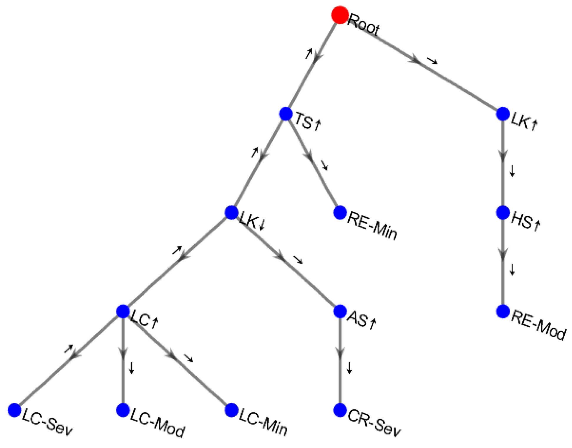
Then, build the FP-Tree in descending order of support, as shown in Figure 10.

Step 2: Mining frequent patterns from the FP-Tree

First, take LC-Sev as an example. Its conditional pattern base is {TS↑, LK↓, LC↑:2}.

Then, through recursive mining, the following frequent patterns are obtained.

{TS↑, LK↓, LC↑, LC-Sev}:2

{TS↑, LK↓, LC-Sev}:2

{TS↑, LC↑, LC-Sev}:2

{LK↓, LC↑, LC-Sev}:2

{TS↑, LC-Sev}:2

{LK↓, LC-Sev}:2

{LC↑, LC-Sev}:2

Step 3: Generate association rules.

For instance, for the rule {TS↑, LK↓, LC↑} → {LC-Sev}:

Support:

$$\sup (\mathrm{TS}\nearrow , \mathrm{LK}\swarrow , \mathrm{LC}\nearrow , \mathrm{LC}\text{-}\mathrm{Sev})={\displaystyle \frac{2}{10}}=0.2$$

Confidence:

$$\mathrm{conf}(\mathrm{TS}\nearrow , \mathrm{LK}\swarrow , \mathrm{LC}\nearrow \to \mathrm{LC}\text{-}\mathrm{Sev})={\displaystyle \frac{\sup (\mathrm{TS}\nearrow , \mathrm{LK}\swarrow , \mathrm{LC}\nearrow , \mathrm{LC}\text{-}\mathrm{Sev})}{\sup (\mathrm{TS}\nearrow , \mathrm{LK}\swarrow , \mathrm{LC}\nearrow )}}={\displaystyle \frac{2/10}{2/10}}=1$$

Degree of lift:

$$\mathrm{lift}(\mathrm{TS}\nearrow , \mathrm{LK}\swarrow , \mathrm{LC}\nearrow \to \mathrm{LC}\text{-}\mathrm{Sev})={\displaystyle \frac{\mathrm{conf}(\mathrm{TS}\nearrow , \mathrm{LK}\swarrow , \mathrm{LC}\nearrow \to \mathrm{LC}\text{-}\mathrm{Sev})}{\sup (\mathrm{LC}\text{-}\mathrm{Sev})}}={\displaystyle \frac{1}{2/10}}=5$$

This rule meets the requirements of the minimum support and minimum confidence thresholds.

Frequent pattern mining aims to identify those driving behavior combinations that frequently co-occur and are closely associated with traffic conflicts, derived from a vast array of driving behavior and traffic conflict data. These combinatorial patterns are crucial for understanding the underlying causes of accidents, predicting traffic conflicts, and formulating targeted safety measures. By excavating frequent patterns, one can uncover behavioral combinations such as “speeding + short headway distance + frequent lane changes”, which exhibit a strong correlation with specific types and severities of traffic conflicts. This directly supports the research objective of reducing traffic accidents on mountainous roads and enhancing overall road safety conditions. It assists transportation management authorities in pinpointing key driving behaviors that warrant monitoring and intervention, thereby facilitating proactive prevention at the source of traffic incidents.

In the FP-Growth algorithm, recursive mining serves as a pivotal step in uncovering frequent patterns. Upon the completion of constructing the FP-Tree, the algorithm embarks on its exploration by commencing with the least frequent behaviors and proceeding in reverse order. Taking “LC-Sev” (severe lane-change conflict) as an illustrative example, we first identify its conditional pattern base—this encompasses other driving behavior sequences associated with “LC-Sev”, along with their respective occurrence frequencies, such as {TS↑, LK↓, LC↑:2}.

Subsequently, a conditional FP-Tree is constructed based on this conditional pattern base; further mining is then conducted within this newly established tree structure. The process of recursive mining perpetually reiterates this cycle, yielding new frequent patterns at each iteration. Each identified frequent pattern represents a potential combination of driving behaviors that could precipitate specific traffic conflicts.

Through recursive mining, the algorithm adeptly extracts all meaningful frequent patterns from the data comprehensively and profoundly. These patterns illuminate the latent relationships among various driving behaviors and their correlations with traffic conflicts—providing crucial data support for subsequent endeavors to generate association rules, assess risks, and formulate safety strategies.

After the calculation, the following key association rules are obtained:

{TS↑, LK↓, LC↑} → {LC-Sev}, sup = 0.2, conf = 1, lift = 5

{TS↑, LK↑, HS↑} →{RE-Mod}, sup = 0.2, conf = 1, lift = 5

{LK↓, AS↑} →{CR-Sev}, sup = 0.2, conf = 1, lift = 5

{TS↑, LK↓} →{RE-Min}, sup = 0.2, conf = 0.5, lift = 2.5

The above rules reflect the strong association between different combinations of driving behaviors and specific types of traffic conflicts. For example, Rule 1 states that a combination of speeding, short headway, and frequent lane changes is likely to result in severe lane-change conflicts; Rule 2 indicates that a combination of speeding, long headway, and sharp braking is likely to cause moderate rear-end collisions.

In the next section, these rules are further evaluated and interpreted to identify the most practical patterns of high-risk driving behavior.

3.2.3. Evaluation of Association Rules

The FP-Growth algorithm can efficiently mine the association rules of driving behavior and traffic conflict, but not all rules have practical significance and application value. To select the key rules with strong correlations and high risk, it is necessary to evaluate the quality of the rules from statistical and professional perspectives. In this study, the Lift index is used to measure the effectiveness of association rules. The formula is as follows:

$$Lift(X\Rightarrow Y)={\displaystyle \frac{Conf(X\Rightarrow Y)}{Sup(Y)}}={\displaystyle \frac{|X\cup Y|\cdot N}{\left|X\right|\cdot \left|Y\right|}}$$

(11)

The degree of enhancement describes the multiple of enhancement of the probability of the occurrence of the rule after the given condition. If the degree of enhancement is greater than 1, this indicates that the occurrence of the former increases the occurrence probability of the latter, and the two are positively correlated; if the lifting degree is less than 1, this indicates that the appearance of the former reduces the occurrence probability of the latter, and the two are negatively correlated. The lifting degree is equal to 1 (the red dashed line in Figure 11), indicating that the former and the latter are independent of each other. Obviously, the higher the lifting degree, the stronger the explanatory power of driving behavior with respect to induction of traffic conflict. Figure 11 shows the promotion degree distribution of some association rules. It can be seen that the combination modes of driving behaviors, such as “TS↑ + LK↓ + LC↑” and “TS↑ + LK↑ + HS”, generally have a high degree of promotion, which is a high-risk incentive for traffic conflict. However, the promotion degree of single behaviors such as “LK↓” and “LC↑” is relatively low, indicating that the interactive superposition of driving behaviors will further magnify the risk of traffic conflict.

To further investigate the statistical significance of the rules, the association rules were tested for confidence difference. For each rule, the confidence interval, [pL, pU], of the probability, p, of traffic conflict was calculated by a binomial distribution and compared with the confidence, p0, of the rule: if p0 > pU, the rule was considered significant at the 95% confidence level.

Table 9. Significance test of key association rules.

Rules	Support	Confidence	Lift	Confidence Intervals	Test Results
{TS↑, LK↓, LC↑} → {CL, Ser}	0.025	0.85	3.72	[0.62–0.78]	Significant
{TS↑, LK↑, HS↑} → {CW, Mod}	0.018	0.78	3.15	[0.55–0.72]	Significant
{LK↓, AS↑} → {CO, Ser}	0.021	0.67	2.58	[0.48–0.65]	Significant
{TS↑, LK↓} → {CW, Min}	0.052	0.63	1.86	[0.46–0.62]	Non-significant

shows the key association rules that partially passed the significance test. It can be seen that these rules not only have a high lift (lift > 2) but also have a significantly higher confidence level than the upper limit of random occurrence probability, indicating that there is a stable and reliable internal correlation between these driving behavior patterns and traffic conflicts, and they are the key objects for prediction and intervention.

3.2.4. Key Driving Behavior Pattern Recognition

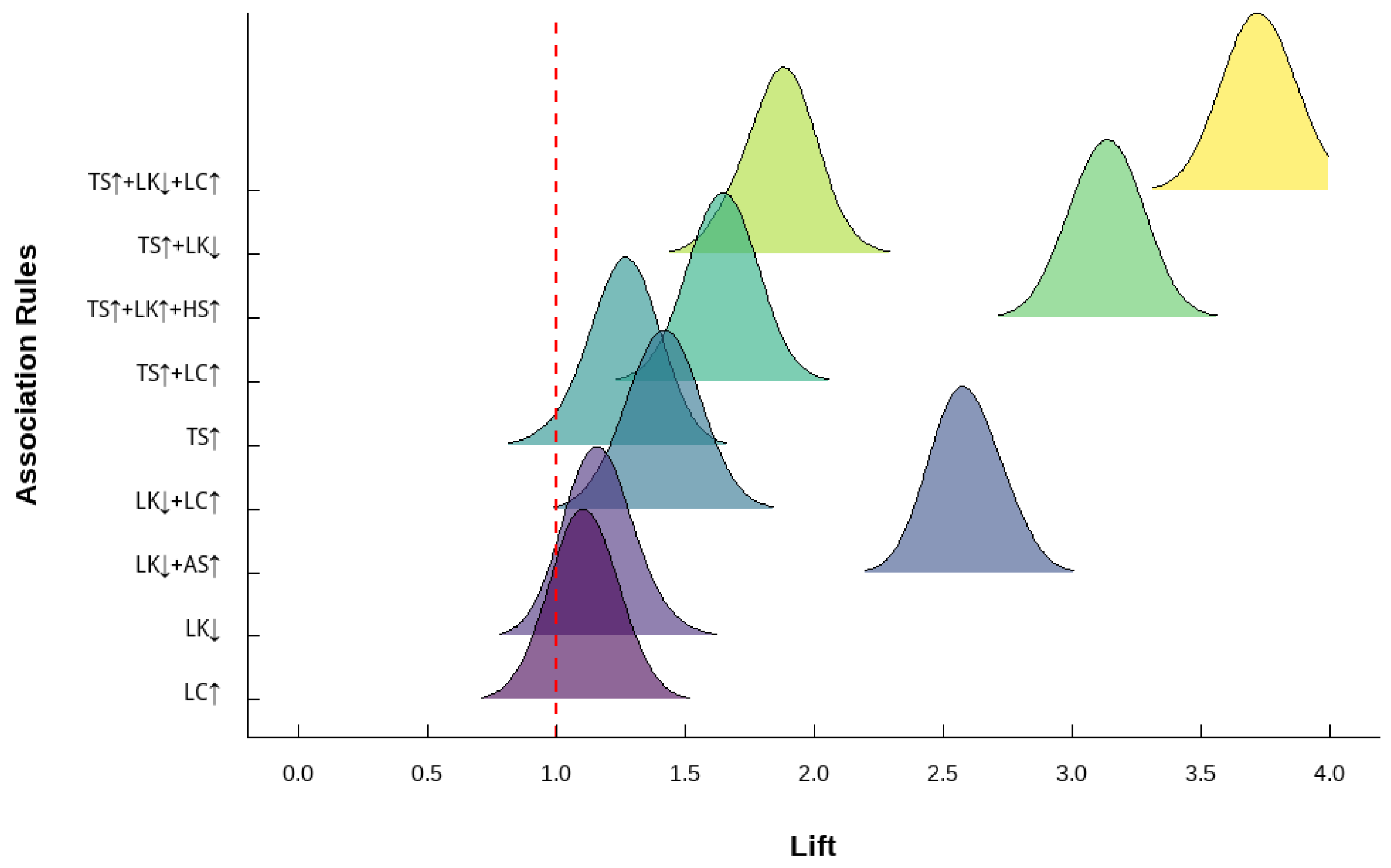
Based on the association rules mined by the FP-Growth algorithm and combined with the enhancement degree and significance test, this paper identifies a series of key driving behavior patterns highly correlated with traffic conflicts, which mainly include the following:

(1) In the mode of speeding + short headway + frequent lane change (TS↑ + LK↓ + LC↑), the probability of lane-change conflict is 3.72 times the average level, and the severity is also high. This indicates that frequent lane changes are very likely to cause vehicle track interleaving and lateral collision under the conditions of overspeeding and short-distance following.

(2) In the mode of overspeed + long front time + sudden braking (TS↑ + LK↑ + HS↑), the probability of rear-end collision is 3.15 times the average level, and most of these collisions are of moderate severity. This indicates that even if the time distance is long, the sudden braking when speeding easily causes the rear car to have no time to react, resulting in a rear-end collision.

(3) In the mode of short headway + rapid acceleration (LK↓ + AS↑), the probability of cross collision is 2.58 times the average level, and most of the collisions are serious. This indicates that rapid-acceleration overtaking is more likely to cause serious collisions at intersections under the condition of short following.

(4) In the mode of speeding + frequent lane change (TS↑ + LC↑), the increase degree in this mode is relatively low (1.86), but it is still the mode associated with a high incidence of rear-end collisions, mostly of a slight degree of seriousness. These results indicate that speeding and lane changing are common causes of traffic flow disorder and potential accidents, and they significantly reduce traffic efficiency, even if no accidents are caused.

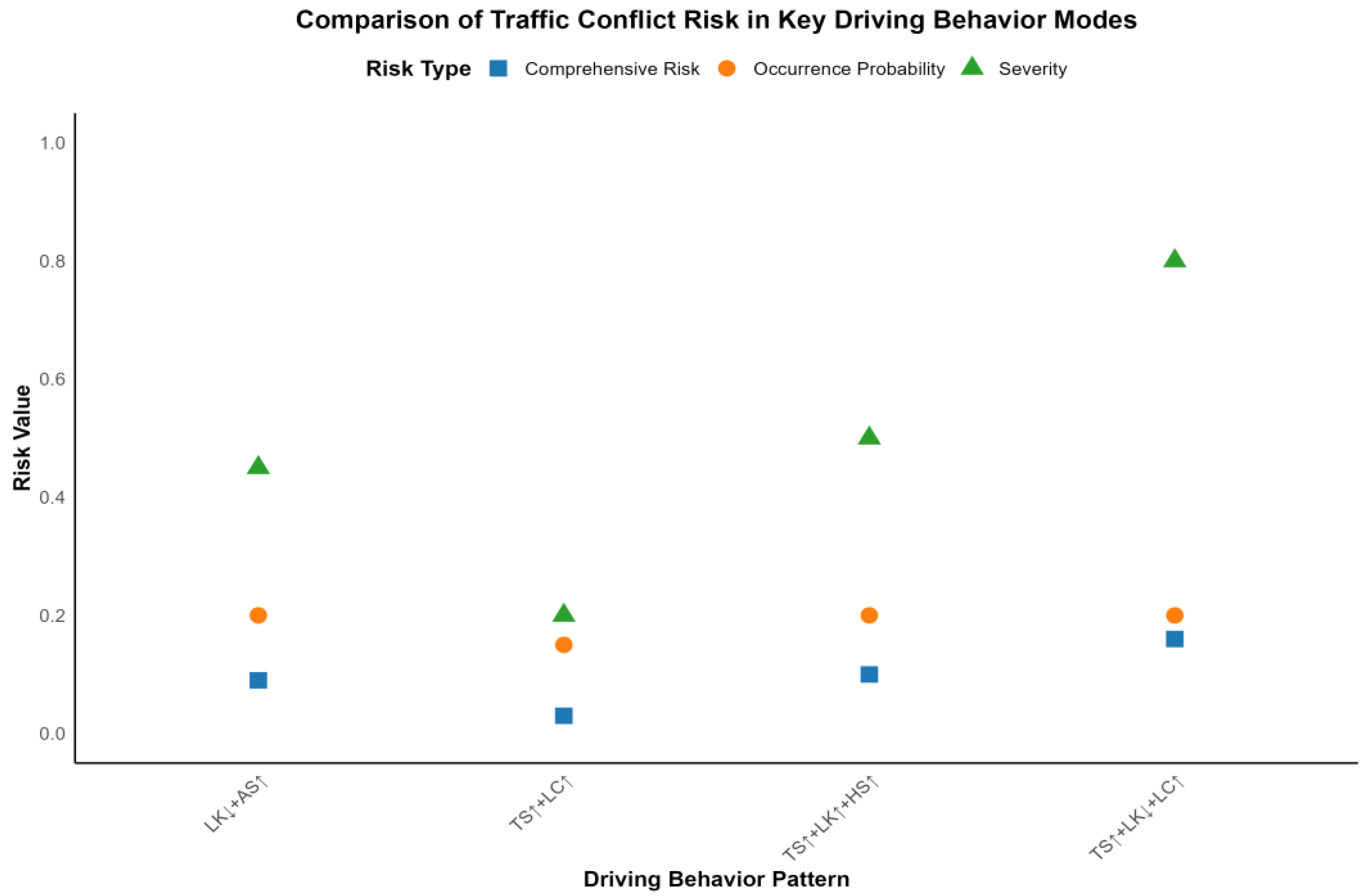
Figure 12 shows the comparison of traffic conflict risks for the above four types of key driving behavior patterns. It can be seen that the mode of “TS↑ + LK↓ + LC↑” has the highest comprehensive risk and that the probability and severity of traffic conflicts are significantly higher than for the other modes, such that it is the illegal behavior that traffic management departments should focus on monitoring and severely crack down on. Other modes, such as “TS↑ + LK↑ + HS↑” and “LK↓ + AS↑”, also have higher comprehensive risks, which are especially likely to lead to accidents of higher severity, which should cause drivers’ vigilance and strengthen legal constraints. Although the “TS↑ + LC↑” mode mostly causes minor collisions, due to its high incidence, it should also be targeted through publicity and education, traffic organization optimization, and other means.

In summary, the FP-Growth algorithm is used to mine association rules from the composite transaction data of driving behavior and traffic conflict and to screen strong association rules through methods such as enhancement degree and confidence tests [42,43], which can effectively identify key driving behavior patterns that cause traffic conflict and realize the prevention and control of traffic accidents from the source of driving behavior. These high-risk driving behavior patterns and the types and severity of conflicts induced by them can be used to guide drivers to improve their safety awareness and correct their driving habits and provide a basis for traffic safety publicity and education. At the same time, this information can also guide the traffic management department to reduce the risk rate of accidents and improve the road environment.

3.3. Prediction Model Performance Results

To comprehensively evaluate the performance of the LSTM traffic conflict prediction model, based on test-set samples, the classification effect of the model was evaluated from multiple perspectives, such as accuracy, recall rate, F1 value, and ROC curve.

Table 10. Classification performance evaluation of LSTM traffic conflict prediction model.

Conflict Level	Sample Size	Recall Rate	F1 Value
Security	4309	0.942	0.934
Slight	267	0.835	0.820
General	175	0.811	0.822
Severe	44	0.750	0.798

shows the evaluation indexes of the model at four conflict levels. It can be seen that the performance of the model at safety, minor, and general levels is relatively balanced; the accuracy and recall rate are generally above 80%, and the F1 value of the comprehensive evaluation index is also high. However, the recall rate of the model is relatively low in the case of a small number of serious grade samples. Overall, the model achieved a classification accuracy of 83.7% on 4795 samples in the test set, and the overall performance was excellent.

An ROC curve and PR curve were drawn, as shown in Figure 13. The area under the ROC curve is 0.912, indicating that the model can balance the TPR (true-positive rate) and FPR (false-positive rate) well and that it has strong classification and discrimination ability. The area under the PR curve is 0.836, indicating that the model can accurately identify conflict samples but also better cover all conflict samples, which has high practical value.

In summary, the traffic conflict prediction model based on LSTM can effectively warn of possible traffic conflict risk during driving by comprehensively considering the heterogeneous characteristics of vehicle movement, driving behavior, road condition environment, and other sources, and it has high accuracy and practicality. The model has a stable training process and excellent test performance, which provides reliable tool support for assisting driving decision-making and indicating hidden safety risks.

4. Discussion

Recent research has demonstrated that intelligent transportation systems have greatly benefited from data-driven approaches to traffic safety. Our findings on driver behavior patterns in mountain roads align with emerging studies showing that behavioral analysis is crucial for accident prevention. Traditional models are giving way to more sophisticated neural networks like LSTM, which can better handle the temporal dependencies inherent in traffic data and capture the complexity of driving environments that leads to frequent traffic crashes. The integration of multiple behavioral indicators (speed, acceleration, headway, and steering) provides a more comprehensive understanding of risk factors than single-parameter analyses.

The application of the FP-Growth algorithm for association rule mining represents a significant methodological advancement over traditional statistical approaches. Figuring out the potential correlation between various risk factors and revealing their coupling mechanisms are effective ways to explore and identify crash causes. Our methodology aligns with recent innovations in data mining applications for traffic safety. These advancements have enabled us to identify complex behavioral patterns that might be missed by conventional analysis methods.

The LSTM neural network model employed in our study parallels recent developments in traffic prediction systems. The practical significance of our research lies in its potential applications for enhancing mountain road safety. The identification of specific high-risk behavioral combinations, particularly the “speeding + short headway + frequent lane change” pattern, provides concrete targets for intervention. This finding corresponds with research by Bogaerts et al. [44], which utilized a graph CNN-LSTM neural network for short- and long-term traffic forecasting based on trajectory data, demonstrating the value of trajectory-based models for safety enhancement.

Recent studies on driving behaviors on curved road sections by various researchers have highlighted how vehicle trajectories are comprehensively affected by the interactions between the vehicle, the driving behavior, and the road environment. Our identification of specific curve entry and exit behaviors aligns with these findings, providing quantitative evidence for the development of targeted safety countermeasures. The predictive model developed in this study offers practical tools for real-time risk assessment. As demonstrated by Yang et al. [45], traffic flow prediction is important for urban planning and traffic congestion alleviation, as well as for intelligent traffic management systems. Our LSTM-based prediction system extends these applications to the specialized context of mountain roads with complex geometries.

Building on our findings, several promising directions for future research emerge. The integration of weather data with behavioral patterns could enhance prediction accuracy. Future studies should also explore the potential of incorporating vehicle-to-infrastructure communication systems to provide real-time warnings based on predicted conflict risks. This approach aligns with emerging Intelligent Transportation System applications that combine predictive analytics with active safety interventions.

The optimization of data mining algorithms for traffic safety analysis represents another valuable research direction. Adapting these optimized algorithms to process continuous streams of driving behavior data could enable more efficient real-time risk assessment systems.

Limitations of our current study include the sample size (30 drivers), which may not fully represent the diversity of driving behaviors in mountain regions. Additionally, our data collection was limited to specific road segments in Hubei Province, China, such that the variations present in mountain roads globally may not have been captured. The driving simulation environment, while highly controlled, cannot perfectly replicate the psychological stress and environmental conditions of real-world driving scenarios. Future research should address these limitations through expanded driver samples, diverse geographical locations, and enhanced integration of simulation with naturalistic driving studies.

In conclusion, our research contributes to the growing body of evidence supporting data-driven approaches to traffic safety, with particular relevance for the challenging context of mountain roads. By combining behavioral pattern analysis with advanced predictive modeling, we have developed tools that can meaningfully contribute to reducing accident risks and enhancing road safety in complex driving environments. The FP-Growth algorithm’s effectiveness in identifying association rules between driving behaviors and conflict types offers a promising methodological approach for future traffic safety research, while the LSTM neural network provides a robust framework for predictive modeling of safety-critical events. Together, these methodological advances offer significant potential for improving road safety management and reducing the occurrence of traffic conflicts in mountain road environments.

5. Conclusions

Our study on mountain roads’ sharp turns reveals four distinct driving patterns, with aggressive styles significantly increasing conflict risk. Most notably, the “speeding + short headway + frequent lane changes” combination elevates the conflict probability 3.72 times above the average. The LSTM prediction model achieved 83.7% accuracy, outperforming traditional methods and offering practical applications for real-time safety systems. Our acceleration-based risk assessment method provides quantitative evaluations for sharp turns, aligning with international standards while uniquely quantifying radius–speed control relationships. Limitations include the limited sample size (30 drivers), the geographic specificity (two Nanjing Province roads), seasonal restrictions (March–August only), simulation–reality gaps, and data integration challenges.

Future work will expand data collection across regions and seasons, integrate findings into vehicle warning systems, develop targeted driver intervention strategies, conduct cross-cultural comparisons, and apply deep reinforcement learning to optimize traffic management. This research provides data-driven foundations for mountain road safety improvements, with the potential for significant practical impact when translated into concrete safety measures.

References

1. Li, W. Rural Road Planning and Management from the Perspective of Rural Revitalization. Sichuan Build. Mater. 2023, 49, 192–194. [Google Scholar]
2. Luo, Y. Problems and Suggestions of Rural Road Traffic Safety Facilities in Mountainous Areas—Taking Zunyi as an Example. Transp. Bus. China 2024, 144–146. [Google Scholar]
3. Wu, Y.; Li, T.; Tian, B. Research on Traffic Accident Prediction of Mountain Expressway Based on Fuzzy Logic. Transp. Sci. Technol. 2024, 115–120. [Google Scholar]
4. Han, W.; Zhao, J.; Chang, Y. Driver behaviour and traffic accident involvement among professional heavy semi-trailer truck drivers in China. PLoS ONE 2021, 16, e0260217. [Google Scholar] [CrossRef]
5. Ji, X.; Xie, S.; Qin, W.; Yang, W.; Hu, C. Dynamic Prediction of Traffic Accident Risk in Dangerous Curved Sections of Mountainous Areas Based on Trajectory Data. China J. Highw. Transp. 2022, 35, 277–285. [Google Scholar]
6. Hu, L.W.; He, Y.; Hou, Z. Multi-Dimensional Coupling Study on Traffic Accident Risk of Highway in Mountainous Areas. China Saf. Sci. J. 2024, 34, 17–27. [Google Scholar] [CrossRef]
7. Branzi, V.; Meocci, M.; Domenichini, L.; Calcinai, M. A Combined Simulation Approach to Evaluate Overtaking Behaviour on Two-Lane Two-Way Rural Roads. J. Adv. Transp. 2021, 2021, 9973138. [Google Scholar] [CrossRef]
8. Rachad, T.; El Hafidy, A.; Idri, A. Factors Associated with Speeding Behavior: Literature Review and Meta-Analysis. Transp. Res. Part F Traffic Psychol. Behav. 2024, 107, 861–875. [Google Scholar] [CrossRef]
9. Raju, N.; Arkatkar, S.; Antoniou, C. Investigating Traffic Safety Reckoning Hyperbolic Driving Following Behavior Using Trajectory Data. Phys. A Stat. Mech. Its Appl. 2022, 606, 128129. [Google Scholar] [CrossRef]
10. Zhu, T.; Yang, H.T.; Zhong, X.Z.; Zou, Y.J. Analysis of Dangerous Following Behavior Characteristics Based on Intelligent Driver Model. Traffic Transp. 2021, 37, 87–91. [Google Scholar]
11. Wen, H.Y.; He, Z.Q.; Li, Q.L. Roads Freight Lane Changing Conflict Prediction and Its Influencing Factors Analysis. J. Jilin Univ. (Eng. Technol. Ed.) 2024, 54, 2827–2836. [Google Scholar]
12. Du, Z.G.; Ni, Y.D.; Mei, J.L. Research Framework of Traffic Safety Improvement Theory and Method in Expressway Tunnel Cluster. J. Wuhan Univ. Technol. (Transp. Sci. Eng.) 2021, 45, 609–617. [Google Scholar]
13. Zhang, W.H.; Tao, H.; Chen, G. Urban Expressway Interchanges Triage Area Traffic Conflicts Forecasting Model. Highw. Eng. 2022, 47, 149–155. [Google Scholar]
14. Nazir, F.; Ali, Y.; Haque, M.M. Effects of Sample Size on Pedestrian Crash Risk Estimation from Traffic Conflicts Using Extreme Value Models. Anal. Methods Accid. Res. 2024, 44, 100353. [Google Scholar] [CrossRef]
15. Yue, Q.; Guo, Y.; Sayed, T.; Liu, P.; Zheng, L.; Lyu, H. Bayesian Hybrid Gamma-GPD Model for Extreme Traffic Conflict Threshold Determination in the Peak Over Threshold Approach. Accid. Anal. Prev. 2024, 206, 107717. [Google Scholar] [CrossRef]
16. Nazir, F.; Ali, Y.; Sharma, A.; Zheng, Z.; Haque, M.M. Car-following crash risk analysis in a connected environment: A Bayesian non-stationary generalised extreme value model. Anal. Methods Accid. Res. 2023, 39, 100278. [Google Scholar] [CrossRef]
17. Wu, P.; Wei, W.; Zheng, L.; Hu, Z.; Essa, M. Cycle-level traffic conflict prediction at signalized intersections with LiDAR data and Bayesian deep learning. Accid. Anal. Prev. 2023, 192, 107268. [Google Scholar] [CrossRef] [PubMed]
18. Lv, N.C.; Peng, L.F.; Wu, C.Z. To Distinguish the Conflict Types of Collision Risk Forecast Model. China J. Highw. Transp. 2022, 35, 93–108. [Google Scholar]
19. Zhao, T.; Zhang, N.; Wang, X.C. A Traffic Conflict Prediction Method for Merging Areas Based on Trajectory Prediction with Graph Neural Network. J. Shandong Univ. (Eng. Sci.) 2024, 54, 36–46. [Google Scholar]
20. Zhang, N.; Liu, B. Research on Active Risk Prevention and Control Method of Intelligent High-Speed Tunnel Based on Traffic Conflict Analysis. Highway 2024, 69, 272–277. [Google Scholar]
21. Karri, S.L.; De Silva, L.C.; Lai, D.T.C.; Yong, S.Y. Classification and Prediction of Driving Behaviour at a Traffic Intersection Using SVM and KNN. SN Comput. Sci. 2021, 2, 209. [Google Scholar] [CrossRef]
22. Formosa, N.; Quddus, M.; Man, C.K.; Timmis, A. Appraising Machine and Deep Learning Techniques for Traffic Conflict Prediction with Class Imbalance. Data Sci. Transp. 2023, 5, 4. [Google Scholar] [CrossRef]
23. Fang, T.; Xu, F.; Zou, Z. Causal Factors in Elderly Pedestrian Traffic Injuries Based on Association Analysis. Appl. Sci 2025, 15, 1170. [Google Scholar] [CrossRef]
24. Chang, J.R.; Chen, Y.S.; Lin, C.K.; Cheng, M.F. Advanced Data Mining of SSD Quality Based on FP-Growth Data Analysis. Appl. Sci. 2021, 11, 1715. [Google Scholar] [CrossRef]
25. Cao, Q.; Zhao, Z.; Zeng, Q.; Wang, Z.; Long, K. Real-Time Vehicle Trajectory Prediction for Traffic Conflict Detection at Unsignalized Intersections. J. Adv. Transp. 2021, 2021, 8453726. [Google Scholar] [CrossRef]
26. Talebloo, F.; Mohammed, E.A.; Far, B. Deep Learning Approach for Aggressive Driving Behaviour Detection. arXiv 2021, arXiv:2111.04794. [Google Scholar]
27. Islam, Z.; Abdel-Aty, M. Traffic conflict prediction using connected vehicle data. Anal. Methods Accid. Res. 2023, 39, 100275. [Google Scholar] [CrossRef]
28. Xu, Y.; Niu, S.L.; Di, Z.W. Anomaly Mining of Ground Meteorological Observation Data Based on FP-Growth Algorithm. Meteorol. Hydrol. Mar. Instrum. 2025, 42, 33–36. [Google Scholar] [CrossRef]
29. Ye, Q.H. Research and Application of FP-Growth Algorithm Based on Data Strong Association. Master’s Thesis, Harbin Commercial University, Harbin, China, 2024. [Google Scholar] [CrossRef]
30. Liang, S.J. High-Dimensional Mixed Attribute Data Mining Method Based on FP-Growth Algorithm. Comput. Technol. Autom. 2024, 43, 88–92. [Google Scholar] [CrossRef]
31. Yan, Z.Y.; Li, L.Q.; Xu, H.J. Photovoltaic Output Prediction Based on Improved Long Short-Term Memory Network Using White Shark Optimization Algorithm. Power Gener. Technol. 2025. [Google Scholar]
32. Wu, J. Research on Flood Forecasting for Small and Medium-Sized Rivers in Shanqiu District Based on Long Short-Term Memory Network. Master’s Thesis, Dalian University of Technology, Dalian, China, 2021. [Google Scholar] [CrossRef]
33. Zhang, J.P. Online Target Tracking Algorithm Based on Visual Short- and Long-Term Memory. Master’s Thesis, Zhengzhou University of Light Industry, Zhengzhou, China, 2023. [Google Scholar] [CrossRef]
34. Liu, F. Traffic Safety Evaluation in Weaving Areas Based on Traffic Conflict Technique. Mod. Bus. Trade Ind. 2016, 37, 198. [Google Scholar] [CrossRef]
35. Wang, H.B.; Su, Y. GNSS Vibration Monitoring Data Based on Kalman Filtering Noise Reduction Processing. J. Jilin Jianzhu Univ. 2024, 41, 68–73. [Google Scholar] [CrossRef]
36. Zeng, L.F. Research on Bridge Acceleration Data Noise Reduction Method Based on Improved LSTM. Master’s Thesis, Guangxi University, Guangzhou, China, 2024. [Google Scholar]
37. Yi, Z.H. Application of Wavelet Analysis in Data Processing of Static Sounding Anomalies. In Proceedings of the 2024 Engineering Survey Conference; Shanghai Chengkun Construction Engineering Consulting Co.: Shanghai, China, 2024. [Google Scholar]
38. Li, F.X.; Zhou, L.; Ding, S.F. Hull Monitoring Data Processing Based on Improved LSTM Exception Handling Method. Ship Eng. 2024, 46, 90–102. [Google Scholar] [CrossRef]
39. Li, G.; Peng, Z.; Wang, Y. Analysis of rear-end collision data in mountainous areas based on random forest and FP growth algorithm. Transp. Sci. Technol. 2019, 5–9. [Google Scholar]
40. Ma, R.M.; Wu, H.X. Research and Application of Association Rule Mining Based on FP-Growth Algorithm. J. Taiyuan Norm. Univ. (Nat. Sci. Ed.) 2021, 20, 19–22. [Google Scholar]
41. Ma, J.; Xie, Y.Q.; Zhang, L.Y. Research on Traffic Accident Data Association Rule Mining Based on FP-Growth Algorithm. Sci-Tech Innov. Prod. 2024, 45, 95–97. [Google Scholar]
42. Wu, Z.l. Based on Data Mining of Power Distribution Network Fault Risk Assessment. Master’s Thesis, South China University of Technology, Guangzhou, China, 2023. [Google Scholar] [CrossRef]
43. Shen, J.W.; Tao, Z.H. Risk Identification, Assessment, and Control of Lifting Operations Based on Apriori Association Rules. Electron. Technol. Softw. Eng. 2023, 202–205. [Google Scholar] [CrossRef]
44. Bogaerts, T.; Masegosa, A.D.; Angarita-Zapata, J.S.; Onieva, E.; Hellinckx, P. A graph CNN-LSTM neural network for short and long-term traffic forecasting based on trajectory data. Transp. Res. Part C Emerg. Technol. 2020, 112, 62–77. [Google Scholar] [CrossRef]
45. Yang, B.; Sun, S.; Li, J.; Lin, X.; Tian, Y. Traffic flow prediction using LSTM with feature enhancement. Neurocomputing 2019, 332, 320–327. [Google Scholar] [CrossRef]
Figure 1. Research framework.
Applsci 15 04891 g001
Figure 2. Location of the experimental section.
Applsci 15 04891 g002
Figure 3. Test instruments.
Applsci 15 04891 g003
Figure 4. Illustration of the construction of an FP-Tree.
Applsci 15 04891 g004
Figure 6. Statistical distributions of input variables for traffic conflict prediction modeling.
Applsci 15 04891 g006
Figure 7. Learning rate and verification accuracy.
Applsci 15 04891 g007
Figure 8. Model training process.
Applsci 15 04891 g008
Figure 9. Early-stopping algorithm flowchart.
Applsci 15 04891 g009
Figure 10. FP-Tree.
Applsci 15 04891 g010
Figure 11. Enhancement degree distribution of association rules.
Applsci 15 04891 g011
Figure 12. Comparison of the risk of traffic conflict for key driving behaviors.
Applsci 15 04891 g012
Figure 13. ROC curve (left) and PR curve (right) of LSTM traffic conflict prediction model on the test set.
Applsci 15 04891 g013