1. Introduction
In this paper, blade tip-timing (BTT) is used for measuring multi-mode rotor blade vibration.
The first tip-timing models work on the assumption that each blade vibrated with the same frequency [
1,
2,
3,
4]. Two simultaneous resonances were analyzed by Gallego-Garrido et al. [
5] using the autoregressive methods BTT.
Beauseroy and Langelle [
6] and Heath [
7] carried out an analysis using a group of sensors to measure multi-mode blade vibration signals. Blade multi-modes using the non-uniform Fourier transform were identified by Kharyton and Bladh [
8]. A sparse reconstruction of the blade tip-timing signal for multi-mode blade vibration monitoring was proposed by Lin et al. [
9].
The application of the sparse representation theorem to find multi-mode blade vibration frequencies with uncertainty reduction was presented by Pan et al. [
10].
Manerowski et al. [
11] presented a method for finding the multi-modes of synchronous and non-synchronous blade vibrations from the tip-timing based on the blade vibration velocity using the Least Squares Technique. This method requires only two sensors in the casing, and a once-per-revolution (OPR) sensor for synchronous and asynchronous vibrations. The rotor blade velocities are obtained from the measured time of rotor blade arrival and used in the functional of the Least Square Technique.
Zhu et el. [
12] also used blade tip-timing vibration velocity obtained from the Taylor series expansion with compressive sensing-based methods in multi-mode blade synchronous vibrations. Five sensors in the casing and a once-per-revolution sensor were used. This method cannot be applied in engineering because of its low accuracy, inefficiency and difficult parameter selection.
Zhu et el. [
13] proposed an acceleration-based blade tip-timing method for synchronous vibration. This method captures rapid changes in vibration, with three sensors in the casing without an OPR sensor.
In all the above papers, the multi-mode analysis assumed the coupling of successive n modes, and only then did a numerical analysis indicate which ones were important.
This paper presents, for the first time, a technique to determine the frequencies and amplitudes of coupled modes in blade vibrations based on the algorithm presented in [
11]. The essence of article [
11] is to search for all harmonic components (amplitudes, frequencies and phases) of the rotor blades using the time of blade arrival measured by sensors in the casing. But the number of harmonics k must be assumed in advance and their number must be high enough to ensure a small calculation error.
In this paper, a technique to determine the frequencies and amplitudes of coupled blade vibration modes based on the algorithm in [
11] is shown. This allows us to determine the precise number of coupled blade vibration harmonics without having to make a prior assumption as to their number. Therefore, the calculation time is considerably shorter. This is the novelty.
The technique is validated a numerical simulation. Here, the experimental and numerical analyses of the 1st compressor rotor blade in an SO-3 engine during run-down are used to determine the multi-mode blade components for synchronous and asynchronous vibrations. The analyses are carried out using two sensors in the casing and an OPR sensor.
2. Methodology for Determining Multi-Mode Blade Vibration Components
The algorithm presented in this paper determines the multi-mode blade vibration components: frequencies ω
i [Hz], a
i and b
i, i − 1, …, k in Equation (1) where the velocity at the time of blade arrival t
v = (t
v1,n, t
v2,n, …, t
v(s−1),n), and n = 1, 2, …, N, N is the number of rotations and s is the number of sensors (see
Appendix A Equation (A11)) is known from the experiment.
Therefore, the measured times of blade arrival are used to determine the number of harmonics on the assumption that the one-mode blade vibration velocity is as follows:
In our numerical calculations, we noticed that by maintaining the single mode (Equation (2)) whilst varying the ω
w and using the algorithm presented in the
Appendix A and [
11], we can obtain local extremes: multiples of the rotation speed frequencies Ω, 0.5Ω, 2Ω, 3Ω, 4Ω, 5Ω, …, ω
w = ω
i + j Ω, j = ±0, 1, 2, …, ω
w = j Ω − ω
i, j = 1, 2, … For us, the ω
i frequencies are important. By assuming a single-mode solution (i.e., Equation (2)), we can obtain the amplitude calculated as a first approximation.
With ω
i and Equation (1), the same algorithm (
Appendix A) can be used to calculate the blade amplitude and phase for each mode. If the amplitudes for ω
i are of a similar order, they show mode coupling. This is a novel approach, which is demonstrated later on in this paper.
3. Validation of the Algorithm by Numerical Simulation
The purpose of this simulation is to verify the algorithm presented in this paper. It was assumed that the rotor speed was Ω = 15,000, rpm = 250 Hz, and the rotor blade vibrated with the assumed parameters in
Table 1, i.e., with 4 harmonics, the velocity amplitudes A
ie, frequencies ω
ie, and phase shift angles φ
ie.
Having assumed the blade vibration parameters (
Table 1), the blade time of arrival was calculated by two sensors mounted at 20 deg. angles in the compressor casing and a blade tip radius R = 0.314 m.
First to be determined were the blade velocity, based on times of arrival t1n, t2n, … then tv1,n, tv2,n, … (Equation (A11)) and velocities v1,n, v2,n, … (Equation (A11)). The above data were determined with the time step Δt = 1 µs (Equation (A3)). These were used to determine the blade vibration parameters a (Equation (A10)), velocity amplitudes Ai, displacement amplitudes Axi, phase angles φi (Equation (A7)), velocity V (Equation (A9)), and displacement X (Equation (A14)).
The velocity amplitudes A
i, frequencies ω
i, and phase shift angles φ
i are compared with A
ie, ω
ie, φ
ie assumed in
Table 1 to validate the algorithm.
Next, we can calculate the accuracy of the vibration velocity amplitude:
where A
ie is the blade amplitude from the simulation (
Table 1) and A
i is the calculated blade amplitude using the algorithm in the
Appendix A.
Phase accuracy:
where φ
ie is the phase from the simulation (
Table 1) and φ
i is the calculated phase using the algorithm in the
Appendix A.
As presented in Equation (1) and in the
Appendix A, the developed method of identifying the blade vibration velocity amplitudes A
i, blade displacements A
xi and phase angles φ
i requires the assumption of vibration frequencies that correspond to the number of harmonics.
In the simulation, it was assumed that the blade vibrated with 4 harmonics for the parameters given in
Table 1.
We used the algorithm (
Appendix A) to calculate the number of harmonics and compared the results with those assumed in
Table 1.
In
Figure 1,
Figure 2,
Figure 3 and
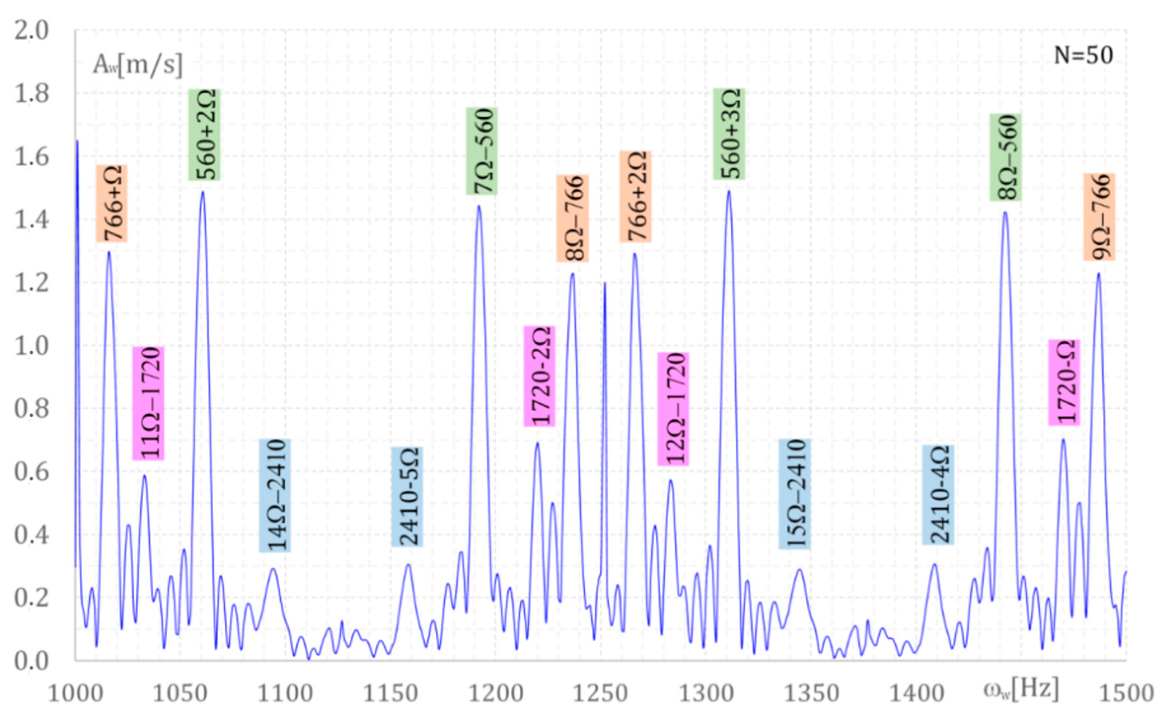
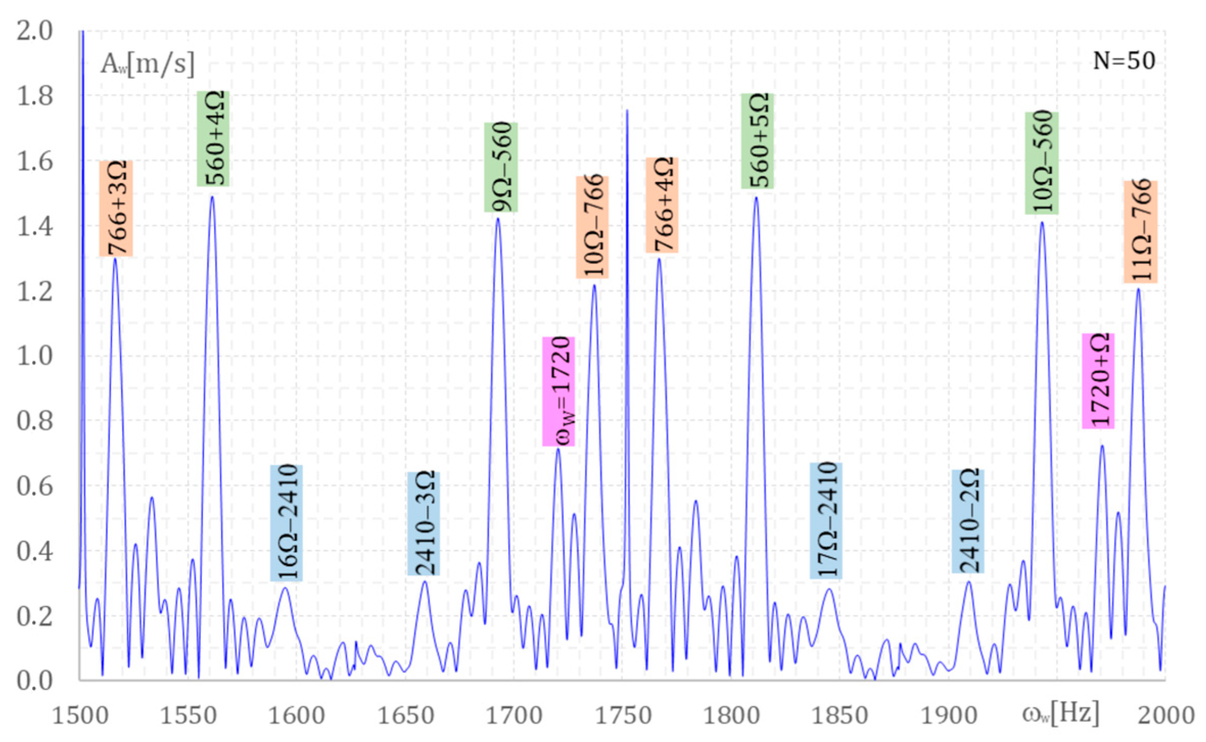
Figure 4, the blade velocity amplitude A
w [m/s] versus frequency ω
w [Hz] are presented with ω
w, varying from 500 Hz to 2500 Hz. These figures show that the local extremes of A
wi occur for frequencies ω
wi. In
Figure 1, the following frequencies [Hz] are seen: 766-Ω, 9Ω-1720, 560, 12Ω-2460, …, 766, 10Ω-1720. The 560 Hz frequency is the same as in
Table 1. Amplitude A
w = 1.57 m/s is close to the 1.50 m/s assumed in
Table 1. The 766 Hz frequency is the same as in
Table 1, amplitude A
w = 1.27 m/s is close to the 1.30 m/s in
Table 1. The frequency 1720 Hz with a 0.66 amplitude in
Figure 3 is the same as the frequency with an amplitude of 0.60 in
Table 1. In
Figure 4, the 2400 Hz frequency is the same as in
Table 1, but the corresponding amplitudes are different, 0.3 and 0.5, respectively.
The calculated amplitudes are close to the assumed amplitudes A
ie (
Table 1).
Next, the algorithm was used for four harmonic frequencies 560, 766, 1720 and 2410 Hz to find the blade velocity amplitudes A
ei, blade displacements A
xi and phase angles φ
i (
Table 2).
Table 2 also shows the influence of the number of rotations N on accuracy in calculating the amplitude ε
iA (Equation (3)) and phase ε
iφ (Equation (4)).
The assumed vibration parameters in
Table 1 are consistent with the calculated vibration parameters in
Table 2, which shows that the algorithm is correct.
The accuracy of the calculated vibration velocity amplitude and phase for: frequency 560 Hz is εiA = −4.7%, εiφ = 5.0%; for 766 Hz, εiA = 5.4%, εiφ = −4.8%; for 1720 Hz, εiA = 10% and εiφ = 7.7% and for 2410 Hz εiA = −14%, εiφ = 19%. These values were calculated for the number of revolutions N = 20 and the accuracy between calculated and assumed velocities σ = 0.23 m/s (Equation (A18)). The accuracy of the vibration velocity amplitude eiA, phase eiφ, and accuracy σ between the calculated and assumed velocities (see Equation (A18)) for N = 25 (σ = 0.79 m/s) and N = 50 (σ = 0.79 m/s are higher than for N = 20 (σ = 0.23 m/s). Therefore, N = 50 will be used in further calculations.
4. Experimental Results of the 1st-Stage SO-3 Engine Compressor During Run-Up
Rotor blade vibrations in the 1st-stage compressor of an ISKRA trainer aircraft SO-3 one-pass engine were measured at Air Force Institute of Technology in Warsaw [
14,
15] using a OPR inductive sensor and two inductive sensors in the casing. Each sensor’s signal frequency range was 0.025–20 kHz. The casing sensors were installed at 12.9 deg (see
Figure A1, ϰ
l+1 − ϰ
l = 12.9 deg) over the 1st stage, radius of a blade tip is R = 0.314 m (the same as in simulation
Section 3).
The SO-3 engine stand consisted of the compressor with seven stages, combustion chamber and one-stage turbine (
Figure 5). Two tip-timing signal processing systems were used to analyzed blade vibration: the SAD-2 [
14,
15] system for laboratory tests and an SNDŁ [
14,
15] system for on-line blade vibration measurement in trainer aircraft. These systems were developed at the Air Force Institute of Technology in Warsaw [
14,
15].
SAD-2 [
15], developed in 1986, measured blade tip displacement in relation to the blade root with two sensors placed, respectively, at the blade tip and root. The sensors on the stand were permanently fixed to the compressor casing or on a special steel frame in the turbine inlet. The system was designed to measure of rotor blades in an SO-3 1st-stage compressor. The number of blades in this stage was 28. This system could monitor and record the displacements of up to 32 blades at various rotation speeds. This technique was next upgraded to the SNDŁ system, which is used in ISKRA trainer aircraft to measure blade vibrations during flights. The SNDŁ system uses two sensors in the compressor casing and indication lamps in the cockpit that switch on when the rotor blade vibration amplitude exceeds 2 mm. In 1988, the SNDŁ system measured 1st compressor-stage blade vibrations in 210 turbojet engines during flight, warning pilots of excessive rotor blade amplitudes.
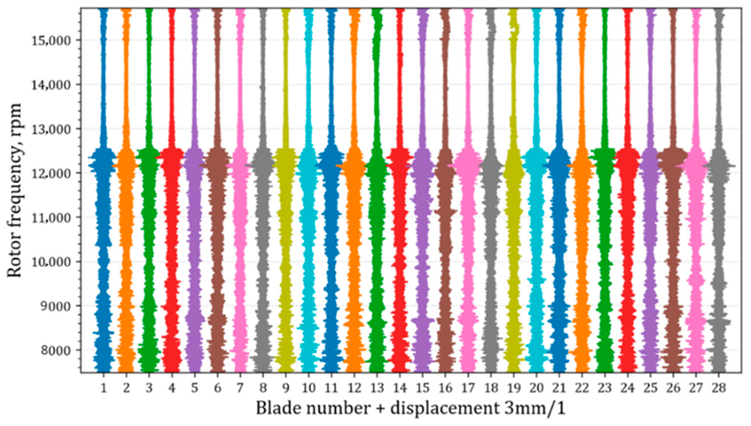
Figure 6 shows the measured displacements of each of the 28 compressor rotor blades rotating from 7500 to 16,000 rpm after de-noising, using Median Absolute Deviation [
16]. The number of blades is on axis x and their rotation speeds are on axis y. The distance between two adjacent blades on axis x (
Figure 6) corresponds to 3 mm blade displacement. This distance is the same between all the adjacent blades. The highest amplitude, 2.5 mm at 12,000 to 12,500 rpm, is caused by rotating stall [
15]. The second highest amplitude, 1.5 mm (15,000 rpm), was caused by forced vibrations in 2 Engine Order (2EO) [
15]. The EO refers to the frequency of oscillations that is a direct multiple of the engine’s rotation speed.
5. Numerical Analysis
This chapter presents a numerical analysis of blade vibrations in the 1st-stage compressor of a one-pass SO-3 ISKRA engine. In several cases, blade failure caused engine damage and plane crashes. In order to obtain a full understanding of the measurement results, it was necessary to carry out numerical analyses using the Finite Element Method (FEM).
The blade was modelled using Solid 45, isoparametric elements with eight nodes [
14,
15]. The mesh was as follows: one element for the thickness, 13 elements for the blade chord, and 10 levels for the blade length. This mesh was sufficient to obtain convergence with the experimental measurements [
15].
The blade was made of 18H2N2 (structural chromium-nickel alloy steel for carburizing). In the calculations, it was fixed in the blade root. Its natural frequencies were compared with experimental ones using strain-gauges and tip-timing analysis [
15].
The free vibration of the rotor blade was calculated using an FEM [
14,
15]. The first four natural frequencies at 15,000 rpm are 509.17, 1527.7, 1863.1, and 3127.8 Hz. From [
15], it was known that the forced and non-synchronous (caused by rotating stall) blade vibration frequencies would be close to their natural frequencies. The rotor blade frequencies in the 1st-stage compressor varied due to manufacture tolerances, e.g., 535, 512, 525, 524, 525, 525, 516, 525, 524, 515, 527, 518, 519, 544, 522, 517, 529, 518, 509, 523, 529, 509, 517, 518, 524, 507, 524, and 525 Hz. These frequencies correspond to the first bending blade frequency.
For Ω = 12,128 rpm, 464, 399, 408, 406, 405, 402, 392, 408, 404, 391, 396, 396, 393, 413, 400, 390, 395, 395, 395, 395, 407, 402, 398, 406, 401, 397, and 395 Hz.
Here, only rotor blade 1 was considered, as an example, but calculations for other blades are analogous.
The blade vibration amplitude A
w and phase φ
w can be found based on Equation (1) for rotation frequencies 250 Hz (15,000 rpm—nominal speed) and Ω = 202.3 Hz (12,138 rpm—non-nominal speed), time step Δt = 1 µs. (Equation (A3)) and [
11] and N = 50.
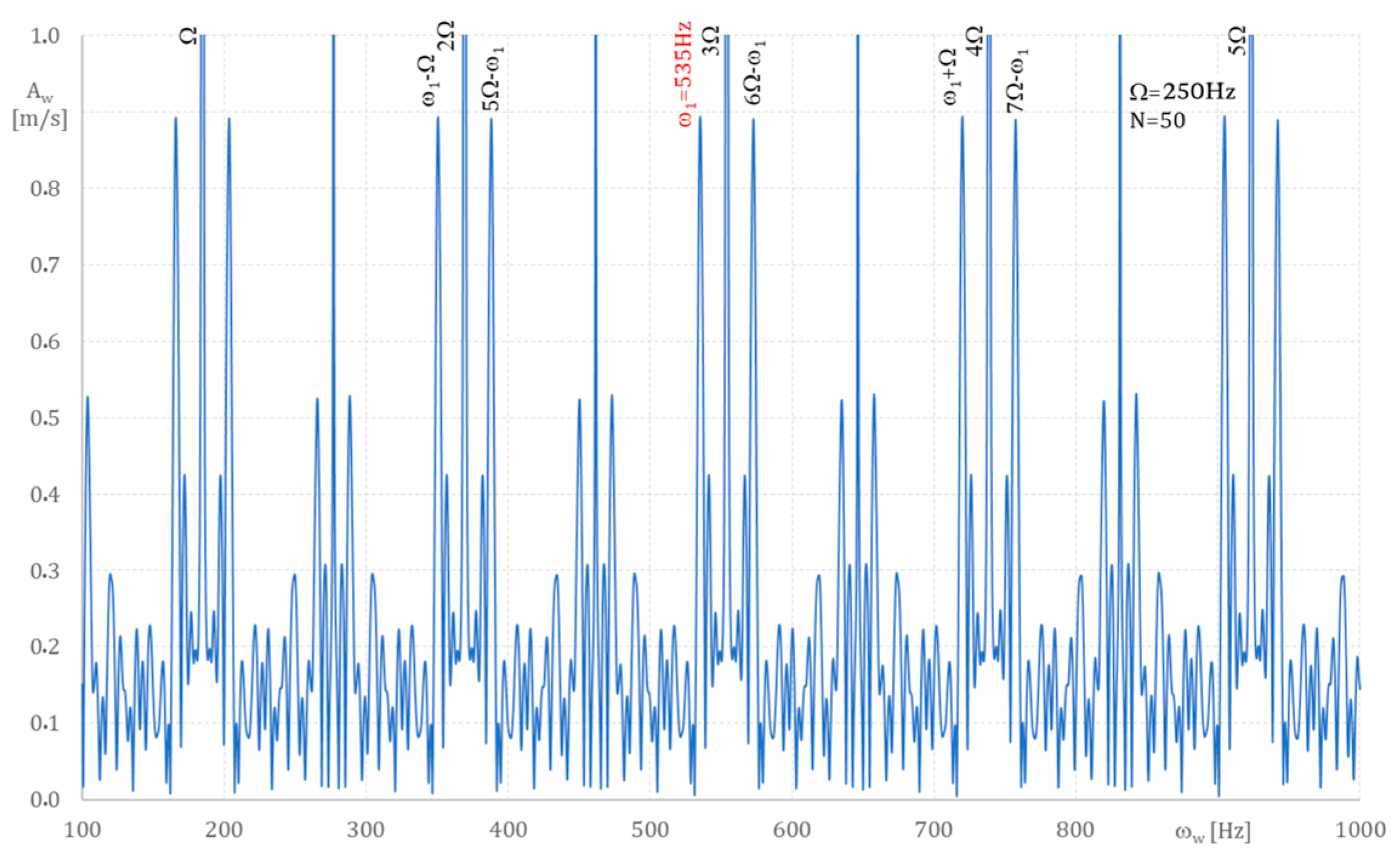
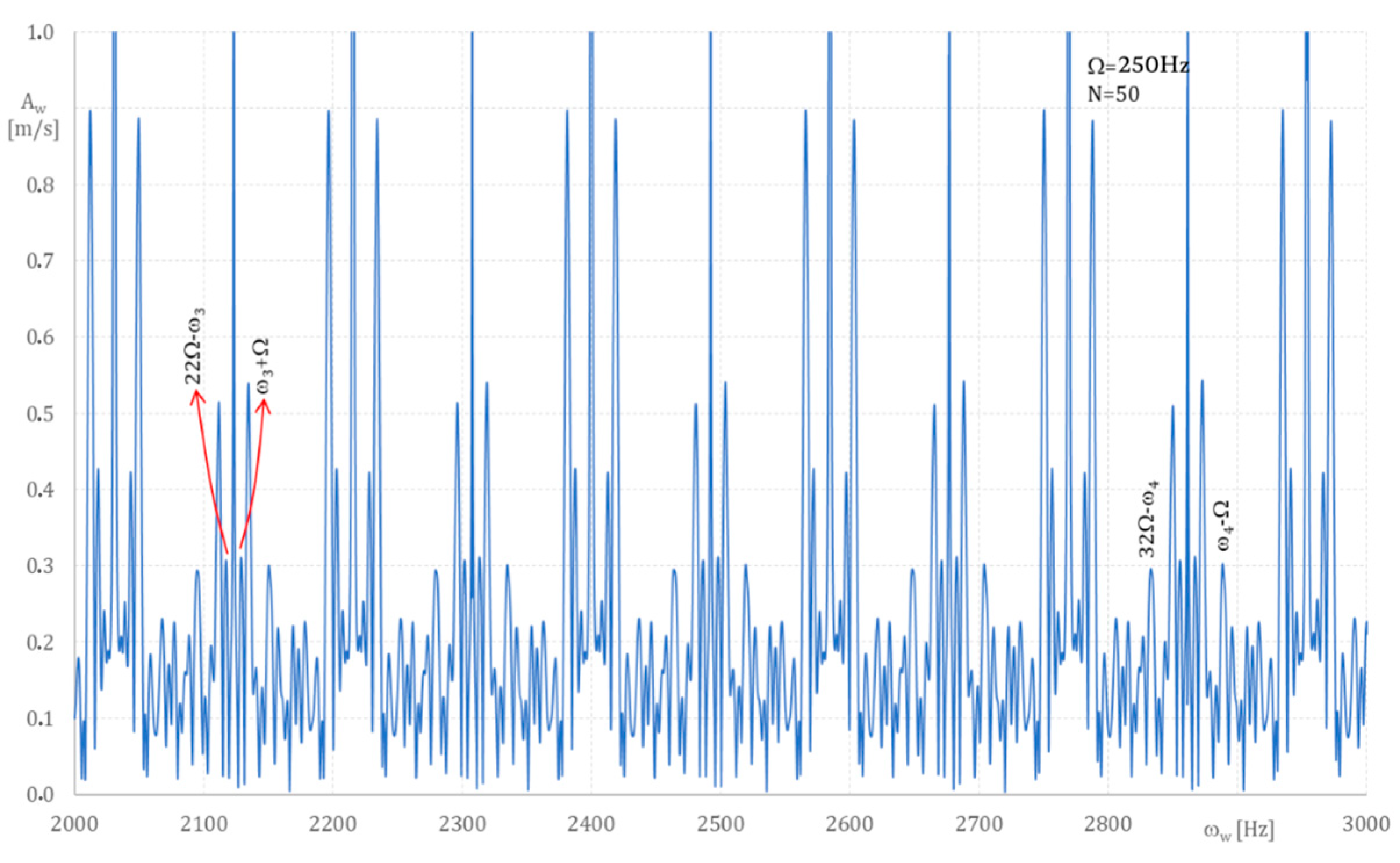
Figure 7,
Figure 8,
Figure 9 and
Figure 10 present blade amplitudes A
w versus various frequencies ω
w (Equation (2)) for rotation speed Ω = 250 Hz. Axis x shows ω
w and axis y shows A
w.
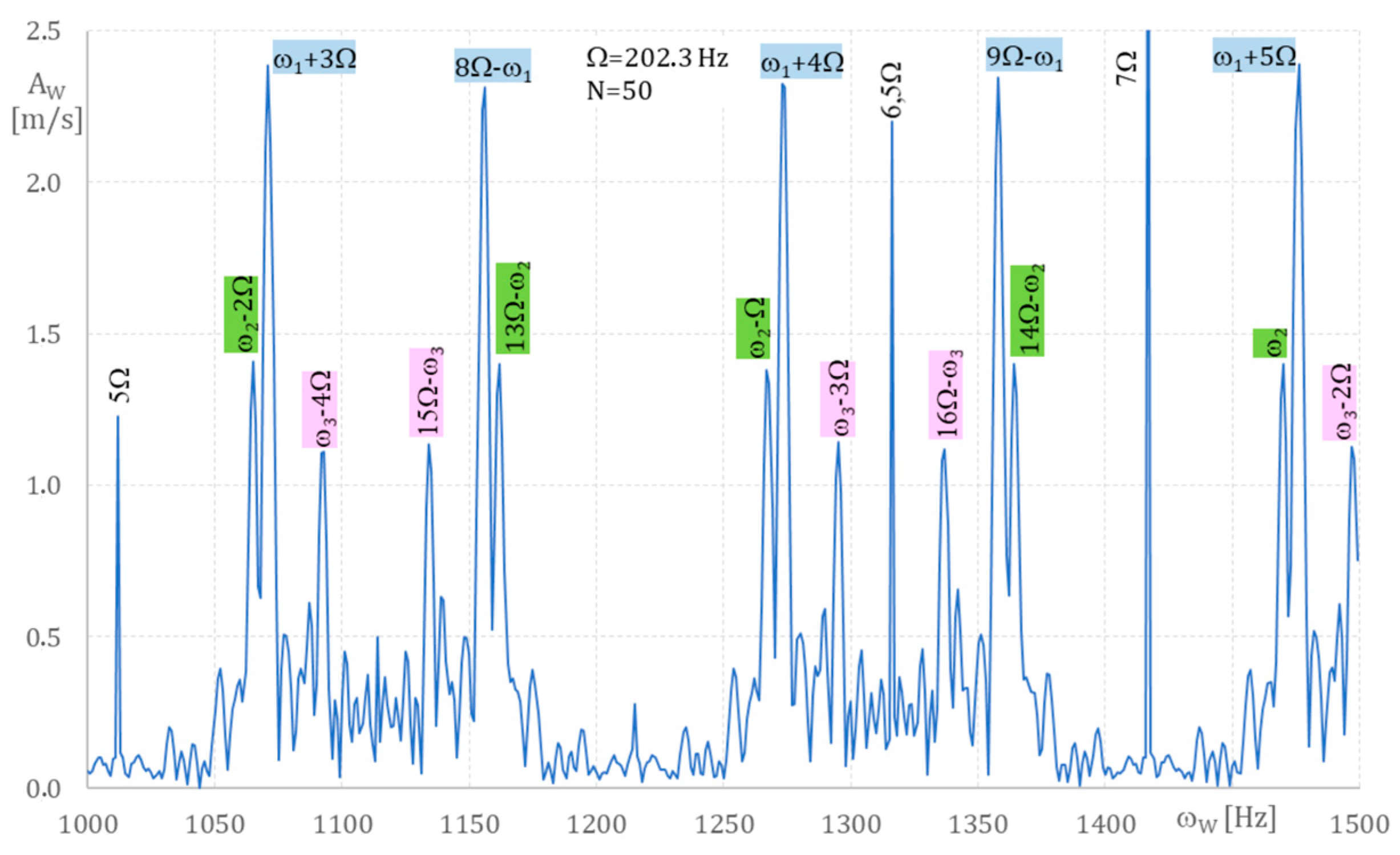
Figure 8, where ω
w is from 1000 Hz to 2000 Hz, shows that ω
2 = 1396 Hz and ω
3 = 1944 Hz.
In
Figure 9, ω
w frequencies change from 2000 Hz to 3000 Hz, but blade vibration components are not found.
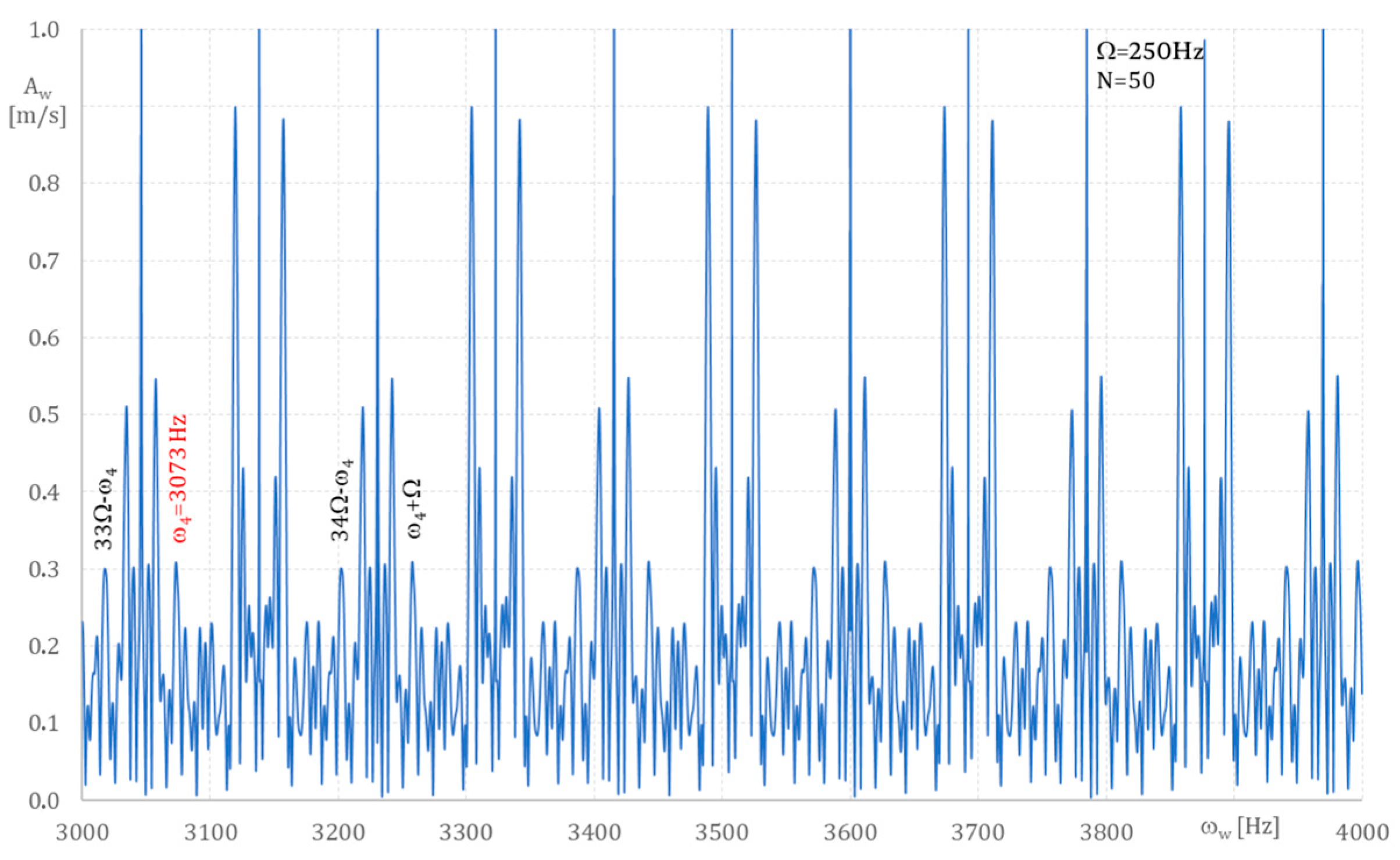
Figure 10, where ω
w changes from (3000 Hz–4000 Hz), ω
4 = 3073 Hz.
Therefore, the spectrum of blade frequencies obtained from
Figure 7,
Figure 8,
Figure 9 and
Figure 10 are ω
1 = 535 Hz, ω
2 = 1396 Hz, ω
3 = 1944 Hz and ω
4 = 3073 Hz. Similarly to
Figure 1,
Figure 2,
Figure 3 and
Figure 4, additional frequencies ω
wl = ω
i ± jΩ, ω
w = jΩ − ω
i (j = 1,2, …, i = 1,2, l = 1, …) also appeared.
From the analysis, the following vibration frequencies were found: ω
1 = 535 Hz, ω
2 = 1396 Hz, ω
3 = 1944 Hz, ω
4 = 3073 Hz for ω
w up to 4000 Hz, assuming one-mode blade vibrations (Equation (2)). So there are four vibration components in Equation (1). These frequencies coincide with the natural blade frequencies calculated using MES [
14,
15]. The
Appendix A Algorithm is again used here to accurately calculate the amplitudes and phases for these frequencies.
Four cases of blade vibration were considered: first, when the blade vibrates only with the first frequency, 535 Hz; second, with two frequencies: 535 Hz and 1396 Hz; third, with three frequencies: 535 Hz, 1396 Hz and 1944 Hz; fourth, with four frequencies: 535 Hz, 1396 Hz, 1944 Hz and 3073 Hz.
In the case of four blade vibration components k (Equation (1)), only the first one has a maximal amplitude of 0.27 mm, resulting from 2EO. For a frequency of 1396 Hz, the blade amplitude is 0.05 mm, 1944 Hz (0.02 mm) and 3073 Hz (0.01). This shows that the rotor blades vibrate predominantly with one component.
Table 3 shows that the higher the number of harmonics, the greater the accuracy of the calculations, though the improvement is only slight.
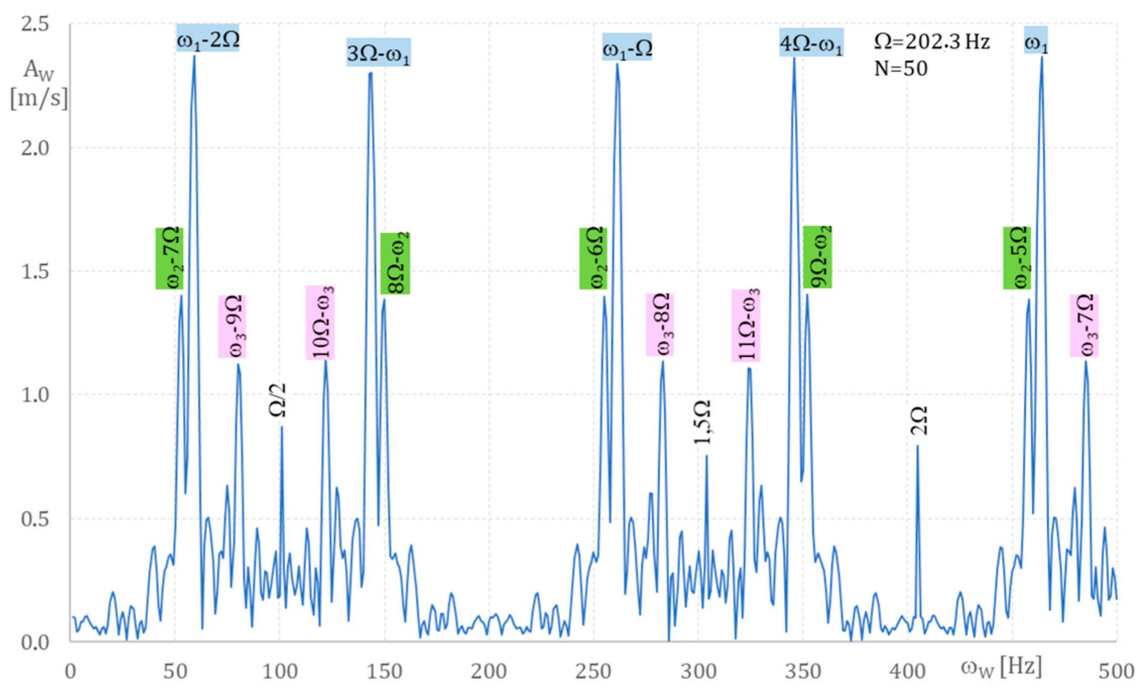
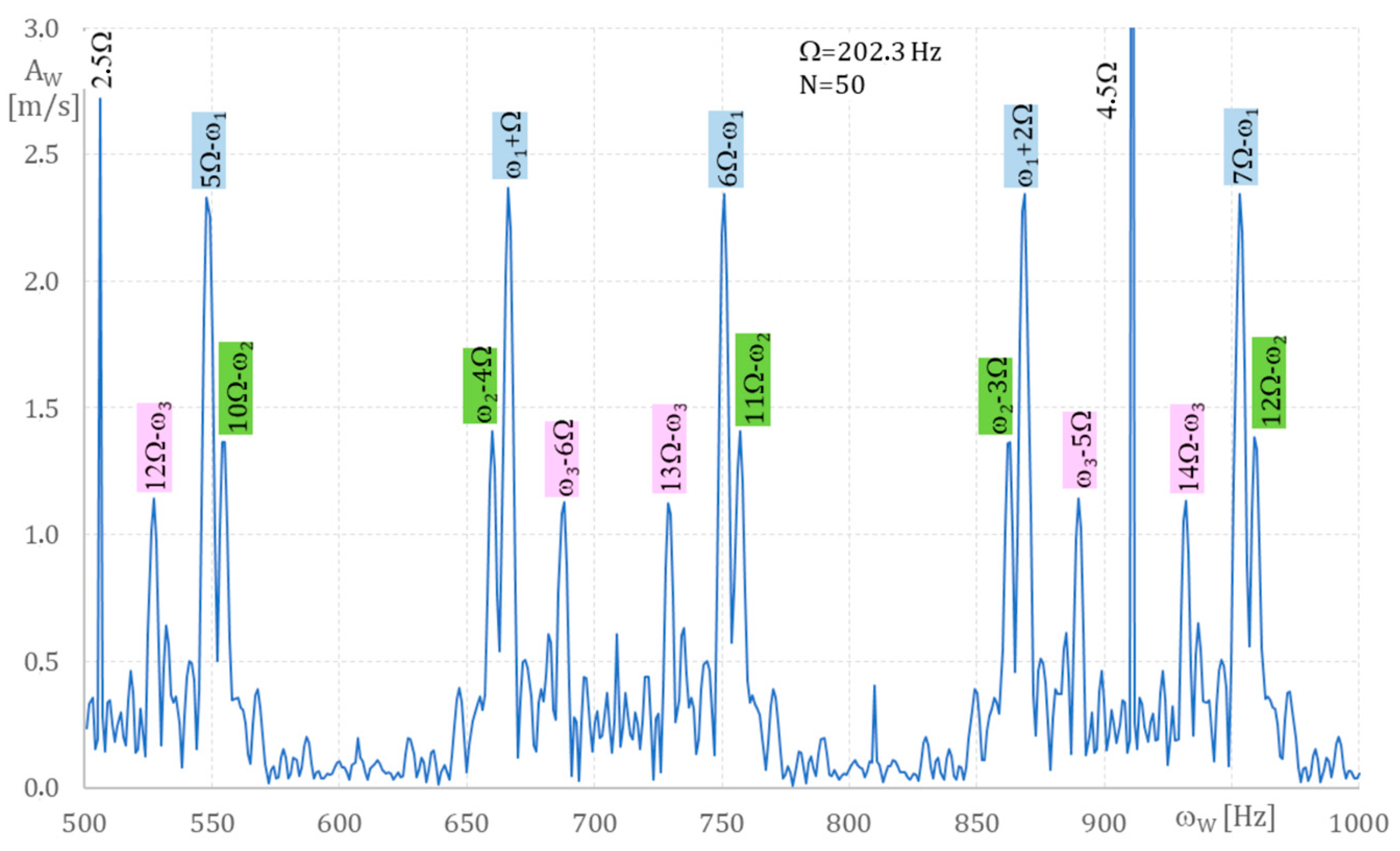
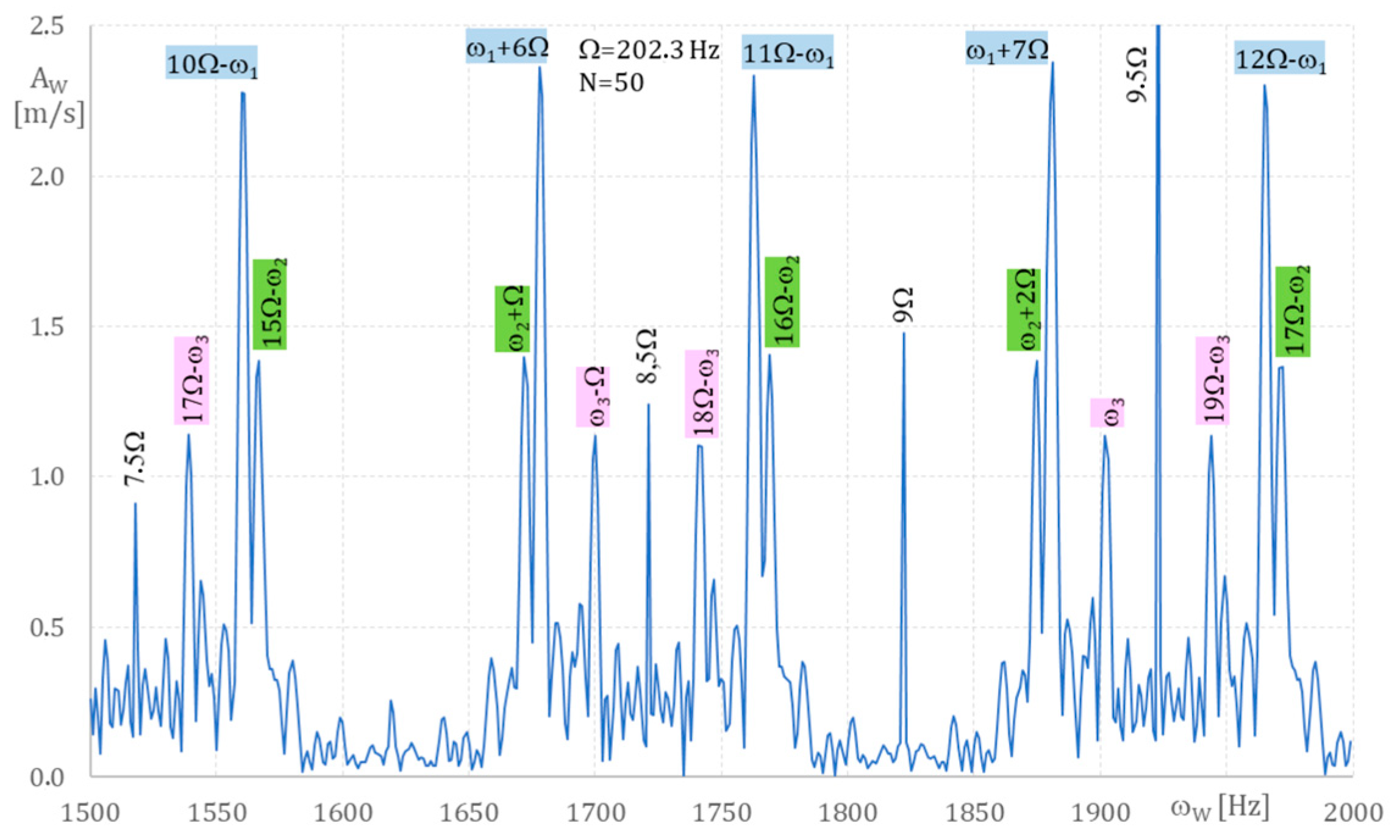
Figure 11,
Figure 12,
Figure 13 and
Figure 14 present blade amplitudes A
w versus various frequencies ω
w from Equation (A15), see
Appendix A, for rotation speed Ω = 202.3 Hz = 12,138 rpm and a time step of Δt = 1 µs. (Equation (A3)) and N = 50. In this case, the blade vibrations are higher than for Ω = 250 Hz (see
Figure 7,
Figure 8,
Figure 9 and
Figure 10) as a result of their non-synchronous motion. The results presented in
Figure 11,
Figure 12,
Figure 13 and
Figure 14 allow us to determine the blade vibration frequencies ω
1 = 464, ω
2 = 1470 and ω
3 = 1902 Hz.
From the analysis, the following vibration frequencies were found: ω
1 = 464 Hz, ω
2 = 1470 Hz, and ω
3 = 1902 Hz when ω
w moves from 500 Hz to 2000 Hz, assuming one-mode blade vibration Equation (2). So there are three vibration components in Equation (1). These frequencies coincide with blade natural frequencies calculated using MES [
16,
17]. As when Ω = 250 Hz, here, too three cases were considered: first, when the blade vibrates only with the first frequency, 464 Hz; second, with two frequencies: 464 Hz and 1407 Hz; third, with three frequencies: 464 Hz, 1407 Hz and 1907 Hz (see
Table 4).
In the case of blades vibrating with three components, k = 3 (Equation (1)), the first, at 464 Hz, has a maximal amplitude of 0.81 mm. The amplitude is higher than for the nominal condition (
Table 3) as a result of rotation stall [
15]. For 1470 Hz, it is 0.10 mm, and for 1902 Hz, it is 0.09 mm, again higher than for nominal conditions due to rotation stall. This shows that in the case of non-nominal conditions, the differences between blade amplitude components are smaller, which is evidence of multi-mode coupling.
This algorithm should be used for all 28 blades to find the maximum blade amplitude, but the conclusion regarding multistage coupling will be the same.
6. Conclusions
The new algorithm presented in this paper determines the multi-mode blade vibration components when the time of blade arrival is known from an experiment. The validation of the algorithm is presented in a numerical simulation, which assumes the blade vibration parameters. This shows the accuracy of the calculated vibration velocity amplitude and phase, as well as the good agreement between the calculated and assumed velocities. The accuracy of the calculations increased with the number of rotations up to N = 50. Therefore, N = 50 was used in further calculations
The 1st-stage compressor rotor blades of an ISKRA trainer aircraft SO-3 one-pass engine were analyzed using tip-timing and the Least Squares algorithm at nominal 15,000 rpm and non-nominal 12,130 rpm.
The rotor blade vibrations were measured [
14,
15] using a once-per-revolution inductive sensor and two inductive sensors in the casing.
In the case of a nominal regime, only one blade component is dominant as a result of 2EO.
In the case of a non-nominal condition, the differences between blade amplitude components are smaller, showing multi-mode coupling as result of rotation stall.
This algorithm can be used for the analysis of steam [
11] and gas turbine blade vibrations, showing whether the blade vibration frequencies in the flow are similar to natural blade frequencies and the number of blade vibration components in the case of multi-mode coupling.


