Frequency-Dependent Acoustic Reflection for Soil Classification in a Controlled Aquatic Environment

Abstract

Seafloor soil classification is essential for marine engineering, environmental monitoring, and geological surveys. Traditional classification methods, such as physical sampling and acoustic backscatter analysis, have inherent limitations, including spatial constraints and inconsistencies in distinguishing sediments with similar acoustic properties. This study uses frequency-dependent acoustic reflection coefficients to investigate a novel spectral-based approach to seabed soil classification. Experiments were conducted in a controlled aquatic environment to isolate the spectral characteristics of two soil types: poorly graded sand (SP) and poorly graded gravel (GP). The research employed calibrated transducers to measure reflection coefficients across the 100–400 kHz frequency range, allowing for a comparative spectral analysis between the two sediments. The results demonstrate that SP and GP exhibit distinct spectral fingerprints, with SP showing higher reflectance across all measured frequencies, while GP displays a more variable spectral response. These findings suggest that frequency-dependent reflectance provides a more sensitive and accurate classification criterion than conventional backscatter intensity analysis. By eliminating environmental variability and focusing on intrinsic soil properties, this study establishes a foundation for automated, non-invasive classification methods that could be integrated into machine learning frameworks for real-time seabed characterization. The proposed methodology enhances the precision of remote sensing techniques and presents significant advantages in offshore engineering, environmental monitoring, and hydrographic surveys. Future research should extend this approach to diverse sediment types and open marine environments to refine and validate its applicability in real-world scenarios.

1. Introduction

Seafloor soil classification represents a fundamental component in various marine applications, with its significance demonstrated across multiple research domains. The characterization of seabed materials has proven crucial for marine engineering projects [1,2], environmental monitoring [3], and geological surveys [4]. The increasing demand for precise seafloor classification has led to significant developments in characterization methodologies over the past decades [5,6,7]. These advances were driven by the need to overcome the limitations of physical sampling methods while maintaining classification accuracy across diverse seabed environments [8,9].

Initially, direct physical sampling methods, including grabbing samples and core drilling, served as the primary means of seafloor classification. Goff et al. [10] demonstrated through extensive field research that physical sampling methods allow precise grain-size distribution analysis and detailed soil characterization. They further showed that acoustic backscatter data can reveal seabed composition patterns, highlighting the potential of remote acoustic sensing as a complementary tool for broader seabed classification. These constraints prompted the development of remote sensing techniques, specifically acoustic methods, for more efficient seafloor classification.

A notable effort to expand acoustic seafloor classification capabilities involved using side-scan sonar (SSS), which provides extensive spatial coverage of the seafloor and is commonly used in habitat mapping applications. The Coastal Water Habitat Mapping (CWHM) project, as reviewed by Penrose and Siwabessy [11], emphasized the potential of SSS as a cost-effective tool for large-scale seabed classification. Unlike single-beam systems, SSS generates high-resolution imagery that can infer seafloor characteristics based on the acoustic texture. However, despite its advantages in providing broad coverage, Penrose and Siwabessy [11] highlighted the key limitations of SSS, particularly its dependence on visual interpretation rather than direct quantitative classification. They noted that while SSS is effective for identifying large-scale geological structures, it struggles to distinguish between sediment types with similar acoustic signatures. Moreover, its performance is highly influenced by factors such as grazing angle, water column properties, and seafloor roughness, leading to inconsistencies in classification. These findings underscore the ongoing challenge of achieving reliable sediment differentiation using acoustic backscatter alone and highlight the need for complementary classification methods that integrate spectral or statistical approaches.

The first advance in acoustic seafloor classification came through multibeam echo sounders, with Hughes Clarke et al. [2] demonstrating their potential for investigating seafloor processes in coastal zones. Their research showed that while these initial acoustic systems could provide basic information about seafloor properties, they were limited by their narrow coverage area and inability to capture detailed spatial variations in seabed characteristics.

Multibeam echo sounders (MBESs) development marked a significant leap forward in remote seafloor characterization capabilities. Brown and Blondel [5] demonstrated MBES’s ability to simultaneously collect both bathymetric data and backscatter information across wide swaths of the seafloor, while Lamarche et al. [6] showed how these systems could maintain high resolution even in deeper waters. Preston [12] further validated MBES’s effectiveness by successfully implementing automated acoustic seabed classification techniques using multibeam data. However, Le Bas and Huvenne [13] identified critical limitations in raw MBES data interpretation, particularly distinguishing between sediments with similar acoustic properties.

While MBES systems represented an advance over single-beam systems, several fundamental limitations persist in their application. Lurton et al. [14] demonstrated that backscatter strength measurements are inherently affected by the angle of incidence, making it difficult to isolate the proper acoustic response of the seafloor material itself. This limitation becomes particularly significant when distinguishing between different sediment types, as the angular dependence can mask subtle differences in material properties. Hamilton and Parnum [15] identified that amplitude-based backscatter analysis struggles to differentiate between sediments with similar grain sizes, noting that multiple factors beyond the sediment composition influence the acoustic response.

De Falco et al. [16] highlighted another critical limitation: the acoustic signal’s interaction with the water column and various environmental factors can significantly impact the received backscatter data. Their research showed that variations in water properties and the presence of suspended particles can alter the acoustic response, making it challenging to establish consistent classification parameters. This observation was further supported by Fezzani and Berger [17], who found that even calibrated seafloor backscatter data could yield inconsistent results when analyzing similar sediment types under different environmental conditions. Eleftherakis et al. [18] emphasized that acoustic methods primarily analyze the total returned signal strength without considering the specific spectral characteristics of various materials interacting with acoustic energy.

The angular range analysis (ARA) technique, initially developed and validated by Fonseca and Mayer [1], provided a methodological framework for analyzing MBES backscatter data. This approach was further refined by Fonseca et al. [19], who demonstrated its effectiveness in linking visual interpretations with acoustic signatures. Simons and Snellen [4] introduced a Bayesian statistical method for classifying seafloor sediments using multibeam backscatter data. By analyzing the acoustic response patterns probabilistically, their approach aimed to improve classification accuracy. However, their research revealed significant limitations in differentiating between sediment types with similar acoustic properties, particularly in areas with mixed sediments or gradual transitions between substrate types.

To address these classification challenges, Fonseca and Calder [20] developed Geocoder, a comprehensive software tool for processing backscatter data from various sonar systems. Lamarche et al. [6] later demonstrated how this tool applies radiometric corrections to account for transmission losses and beam-pattern effects, aiming to produce standardized backscatter measurements. However, despite these processing advances, Lurton et al. [13] found that a fundamental challenge remained: the acoustic response was still influenced by factors external to the sediment properties, such as water column variations and incident angle dependencies.

In summary, seafloor soil classification is critical for marine engineering, environmental monitoring, and geological surveys. Traditional classification methods, such as physical sampling and acoustic backscatter analysis, face persistent challenges. Physical sampling methods, including grab sampling and core drilling, provide high-resolution grain-size distribution data but are time-consuming, labor-intensive, and limited in spatial coverage [10]. Acoustic-based techniques have been developed as efficient remote-sensing alternatives, including side-scan sonar (SSS) and multibeam echo sounders (MBESs). Still, they rely primarily on backscatter intensity, which is affected by environmental variables such as grazing angles, water column properties, and sediment roughness [11,14]. As a result, these methods struggle to differentiate sediments with similar grain sizes and composition, leading to classification inconsistencies [15,17]. Recent research has explored spectral-based methods as an alternative to seabed classification. Studies by [21,22] have demonstrated the potential of spectral acoustic analysis to distinguish between sand and sandstone using frequency-dependent backscatter characteristics. However, prior studies have focused on differentiating rock from sediment rather than more subtly classifying soils with similar grain sizes but different grading properties. Additionally, many spectral studies lack controlled experimental conditions, making it difficult to isolate the intrinsic acoustic response of sediments from external environmental influences. Hence, a systematic investigation is needed to assess whether spectral acoustic analysis can reliably classify sedimentary soils with subtle physical differences. Specifically, the research should focus on isolating intrinsic spectral characteristics in controlled environments and establishing spectral fingerprints for different soil types.

The primary objective of this study is to develop a non-invasive, spectral-based approach for soil classification in aquatic environments. This study aims to achieve the following:

✓

Establish distinct spectral fingerprints for poorly graded sand (SP) and poorly graded gravel (GP) using frequency-dependent acoustic reflection coefficients.

✓

Evaluate the reliability of spectral analysis in distinguishing soil types with similar grain sizes but different grading properties.

✓

Develop a controlled experimental methodology that eliminates environmental variables and isolates sediment-specific spectral responses.

✓

Lay the foundation for automated classification by providing spectral data that can be integrated with machine learning models for seabed characterization.

✓

By achieving these objectives, this research will advance seabed classification techniques, providing a more accurate and reproducible alternative to traditional acoustic intensity-based methods.

To achieve the outlined goal, this study will undertake the following key tasks:

✓

Experimental Setup in a Controlled Environment

✓

Conduct spectral acoustic measurements in a freshwater tank to eliminate water column distortions.

✓

Use calibrated transducers to measure frequency-dependent acoustic reflection in the 100–400 kHz range.

✓

Comparative Spectral Analysis of SP and GP Soils

✓

Measure and analyze the spectral reflection properties of poorly graded sand (SP) and poorly graded gravel (GP).

✓

Identify and quantify the spectral differences between the two soil types.

✓

Validation of Spectral Signatures for Classification

✓

Evaluate the repeatability and robustness of spectral fingerprints.

✓

Assess whether the spectral differences provide a reliable classification criterion.

✓

Assessment of Potential for Automated Classification

✓

Explore how spectral reflection coefficients can be used as input features for machine learning models in future classification frameworks.

By systematically executing these tasks, this study aims to establish spectral acoustic analysis as a viable, scalable, and non-invasive method for soil classification in aquatic environments.

The present research is conducted in a controlled laboratory environment, ensuring the precise measurement of acoustic interactions with sediment samples. The controlled setting eliminates unpredictable marine influences, allowing an accurate assessment of intrinsic spectral properties. The findings from this study will provide the first experimentally validated spectral fingerprints for sediment classification, demonstrating whether spectral-based acoustic reflectance analysis can reliably distinguish between similar sediment types. The results presented in the following sections will detail the spectral response of SP and GP soils, compare their reflection coefficients, and evaluate the effectiveness of this approach in differentiating sedimentary soils based on acoustic energy interactions. The Section 4 will critically analyze these findings to assess their implications for marine geophysics and remote seabed classification.

2. Materials and Methods—Acoustic Spectrum Characterization

In this study, the spectrum of the acoustic reflection coefficient is defined as the ratio between the energy leaving the soil and the energy entering it in an aqueous environment. This characterization quantifies energy absorption within different soil types, enabling classification based on spectral response. The fundamental assumption is that distinct soils exhibit unique frequency-dependent attenuation patterns, which can be identified by analyzing energy transformation between the incident and reflected acoustic waves.

2.1. Materials

Two soil types were selected to investigate spectral acoustic reflection characteristics: a fine-grained, non-cohesive sand and a coarser-grained, granular gravel. Both were analyzed using standard sieve tests to determine their particle-size distribution and gradation characteristics.

Poorly graded sand (SP):

The SP soil consisted of quartz-based, sub-angular particles with minimal fine content. The particle size distribution included D10 = 0.30 mm, D30 = 0.35 mm, D50 = 0.40 mm, and D60 = 0.45 mm. The calculated uniformity coefficient (Cu) was 1.50, and the coefficient of curvature (Cc) was 0.91, confirming its classification as poorly graded under the Unified Soil Classification System (USCS). The sand was oven-dried prior to testing and exhibited high permeability and low angularity.

Poorly graded gravel (GP):

The GP soil sample comprised sub-rounded limestone fragments with no fine material and high void content. The grading analysis yielded D10 = 2.8 mm, D30 = 4.0 mm, D50 = 5.4 mm, and D60 = 6.0 mm, resulting in a uniformity coefficient (Cu) of 2.14 and a coefficient of curvature (Cc) of 0.95. These values are consistent with a poorly graded coarse gravel, confirming its USCS classification. Like the sand, the gravel samples were oven-dried before testing to ensure consistency in the acoustic measurements.

Full grading curves for both soils are provided in Figure 1 and Figure 2.

• Poorly graded sand (SP)—a fine-grained, non-cohesive sediment with uniform particle size. The grading curve for receiving SP soil appears in Figure 1.
• Poorly graded gravel (GP)—a coarser-grained material with higher permeability and varied particle distribution. The grading curve for receiving GP soil appears in Figure 2.

The aim is to analyze the frequency-dependent acoustic characteristics of the two soil types, by measuring how much of the transmitted energy is reflected back at each frequency. In this study, the term “spectral differences” refers to differences in the pattern and intensity of acoustic reflection across the tested frequency range (100–400 kHz). These differences reflect the unique way each soil interacts with sound energy at different frequencies and form the basis for distinguishing between the materials.

2.2. The Parameters Under Study

To quantify the acoustic reflection spectrum, the following energy parameters were calculated:

Incident Energy $I_1(f)$—the energy reaching the soil surface at a specific frequency.

Reflected Energy $I_0(f)$—the energy leaving the soil surface post-interaction at a specific frequency.

It can be assumed that the ratio between these values describes the soil’s frequency-dependent reflection. To accurately determine the acoustic reflection spectrum, the incident energy reaching the soil surface $I_1$, must first be quantified. This energy represents the total acoustic energy propagating through the water before interacting with the soil. The incident energy at each frequency is computed by integrating the squared measured amplitude of the incident signal over time, following the fundamental relation that appears in Equation (1) [23]:

$$I_1(f)={\int }_{t_{start}}^{t_{end}}{A(f,t)}^2·dt$$

(1)

where

$I_1(f)$ is the total acoustic energy impacting the soil surface at a given frequency;

$A(f,t)$ represents the normalized amplitude of the transmitted wave; and

$t_{start}$ and $t_{end}$ denote the time window corresponding to the transmission period at the selected measurement location.

2.3. Experimental Setup

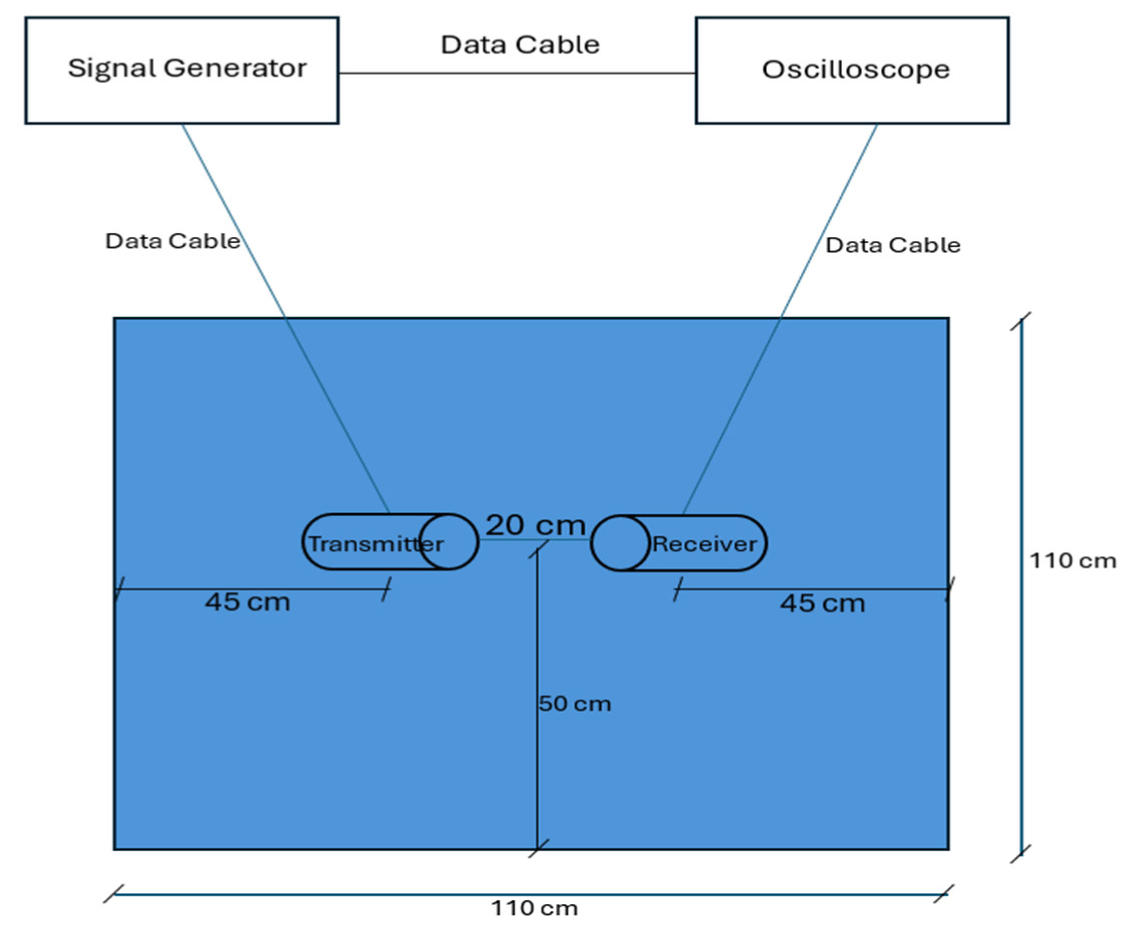
This computation must be performed independently for each tested frequency, covering 100 kHz to 400 kHz in 10 kHz increments. To measure $A(f,t)$ in the ranges mentioned above, two transducers were placed facing each other at 20 cm in a water tank, and the readings in the frequency range 100–400 kHz were recorded (see Figure 3 for the schematic diagram showing the experimental setup for determining the energy defined as $I_1$) Greenberg et al. [24] presented the methodology in detail and briefly described here.

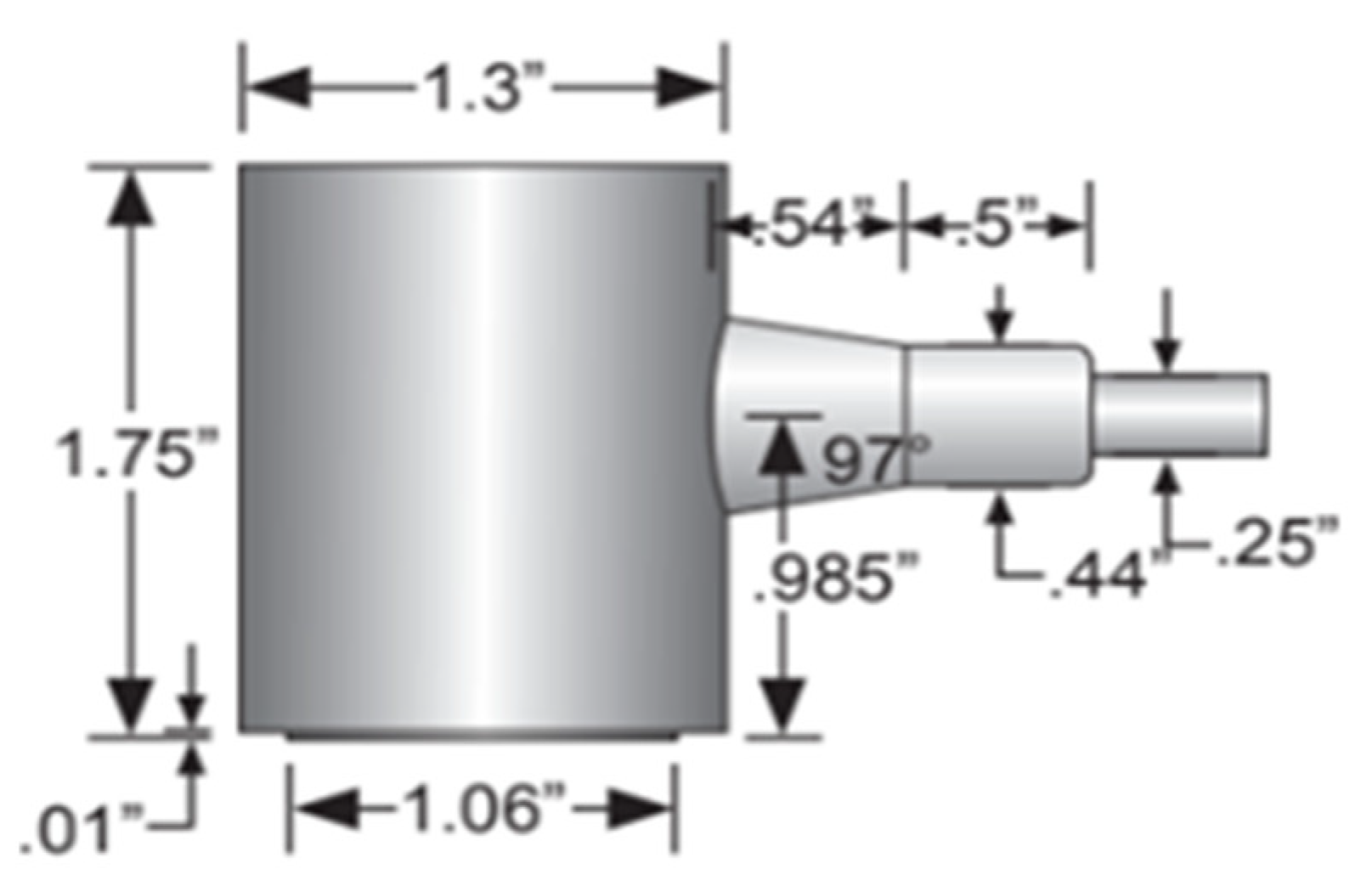
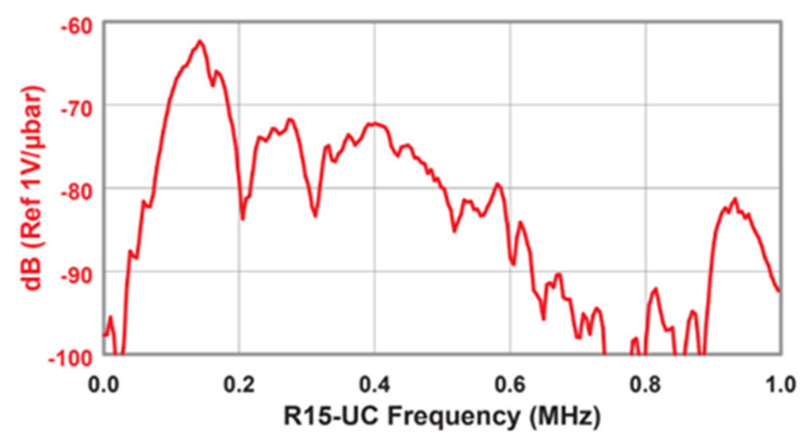
Figure 4 and Figure 5 show the transducer’s dimensions and their reception curve.

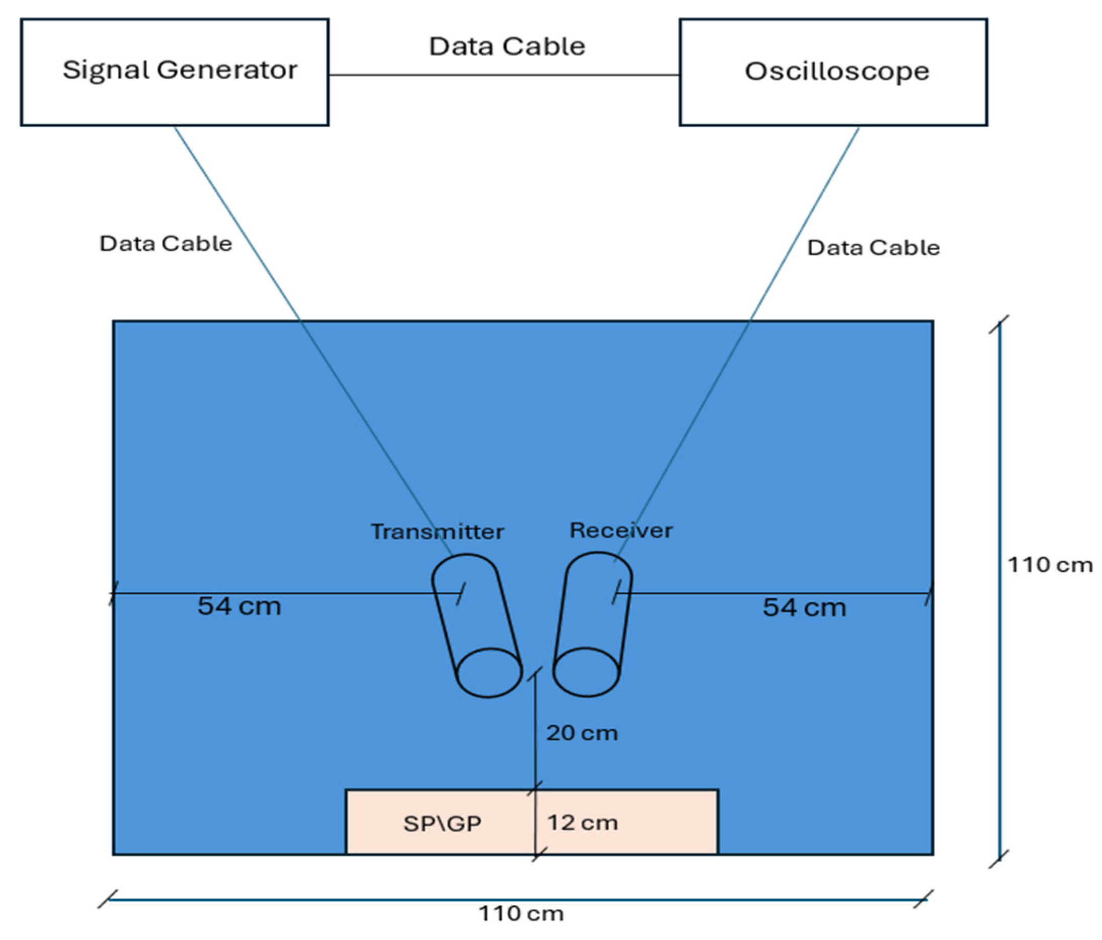
The experimental setup for measuring the energy $I_0$ reflected from soil samples was designed such that the incident energy $I_1$ reaching the soil samples will be identical to the energy measured in the previous study [24]. Two transducers were positioned next to each other, facing down in a water tank at a fixed distance of 20 cm from the soil sample placed at the bottom of the tank. The positioning of the transducers was such that the reflected signal reached the recording transducers separately from the direct arrival and reflections from the boundaries. The position of the transducer in the water was such that the direct arrival at the receiver would be completely isolated in the time domain from any reflection from the boundaries. Also note that the distance between the transducers and the soil samples in terms of the acoustic wavelength is significantly greater than 4.83 cm, corresponding to the far field threshold. The thickness of the samples was such that the whole signal was reflected from the top of the sample before the signal reached the bottom of the sample, such that the reflections of the top and bottom soil boundaries did not overlap. The experimental setup is presented schematically in Figure 6.

For each soil type, 31 acoustic readings were performed per sample, over 10 samples per soil type, at frequency intervals of 10 kHz within the 100–400 kHz range. The reflected signal was recorded at each frequency, and then the gain function developed by Greenberg, Kushnir, and Frid [24] was applied to obtain $I_0$ (stacked over the 10 samples) and allowing (together with $I_1$) for subsequent reflection coefficient spectrum calculation.

For completeness, the gain function by Greenberg et al. [24] for determining reflected energy based on the recorded energy is outlined next:

$$log\left(I_0\right)=C_{1}log\left(I_i\right)+C_{2}log\left(R_i\right)+C_3{f}^2\left(R_i-1\right)+C_7+C_8{I}_i+C_{9}f+C_{10}f\left(R_i-1\right)$$

(2)

where

• $I_0$ = the energy coming out of the ground after performing amplification to $I_i$;
• $R_i$ = distance between the transmitting transducer and the ground, the same as between the ground and the receiving transducer;
• $I_i$ = The energy that reaches the receiving transducer after receiving an acoustic reading from the ground; and
• $C_1,C_2,C_3{,C}_7,C_8, C_9, C_{10}$ = are the constant coefficients given in

  Table 1. Trained coefficients for Equation (1).

  Coefficient	Value
  C1	1.032682
  C2	0.319061
  C3	0.186415
  C7	−4.79983
  C8	−0.04989
  C9	0.103657
  C10	−0.23531

  , which were determined by Greenberg et al. [24].

Please note that each value on the right side of Equation (2) is a normalized one by the following equation [25]:

$$X^{\prime }={\displaystyle \frac{X-\mu }{\sigma }}$$

(3)

where

X is the original value of the feature for a specific training example;

μ is the mean of the feature values over all the training examples;

σ is the standard deviation of the feature over all the training examples; and

X′ is a specific training example’s normalized (standardized) value.

The standard deviation and mean values of each feature appear in

Table 2. The standard deviation and mean values of each feature.

Feature	Mean Value	Standard Deviation Value
$log\left(I_0\right)$	−5.45121	0.87433
$log\left(R_i\right)$	1.13261	0.131513
$f^2\left(R_i-1\right)$	940,386.9	707,901.4
$I_i$	71,307.3	45,476.67
$f$	${2.87·10}^{-5}$	${8.31·10}^{-5}$
$f\left(R_i-1\right)$	251.5328	89.65783

and should be applied whenever using the trained nonlinear regression model by Greenberg et al. [24] for calculating $I_0$:

Environmental conditions such as temperature and water composition were maintained at the same conditions as in [24] to ensure the validity of the gain function and trained coefficients.

3. Result: Spectral Analysis and Data Visualization

Figure 7, Figure 8, Figure 9 and Figure 10 show the reflected spectrum graphs of SP and GP: Figure 7 and Figure 8 portray the reflection spectra for poorly graded sand and gravel, respectively. Figure 9 and Figure 10 enable the comparison of both spectrums in a non-normalized and normalized manner. Visualization provides insight into how different soil compositions attenuate and reflect acoustic energy. By comparing spectral trends, this study aims to establish distinct frequency-domain signatures for each soil type, facilitating their classification.

Due to the different values of the spectra of the two different soils, we also normalized the graphs shown in Figure 7 and Figure 8 by dividing the total values of each graph by its highest value. By doing this, it is possible to see the behavior of the reflected spectrum of the two types of soils in the same graph and examine it.

The findings show a consistent difference in reflection intensity between SP and GP soils. SP exhibits higher reflectance values across all measured frequencies, while GP demonstrates a more variable spectral response. These findings provide a basis for further discussion of the physical mechanisms influencing spectral variations, comparison with previous studies, and potential applications of spectral-based acoustic classification.

4. Discussion

4.1. Significance of the Findings

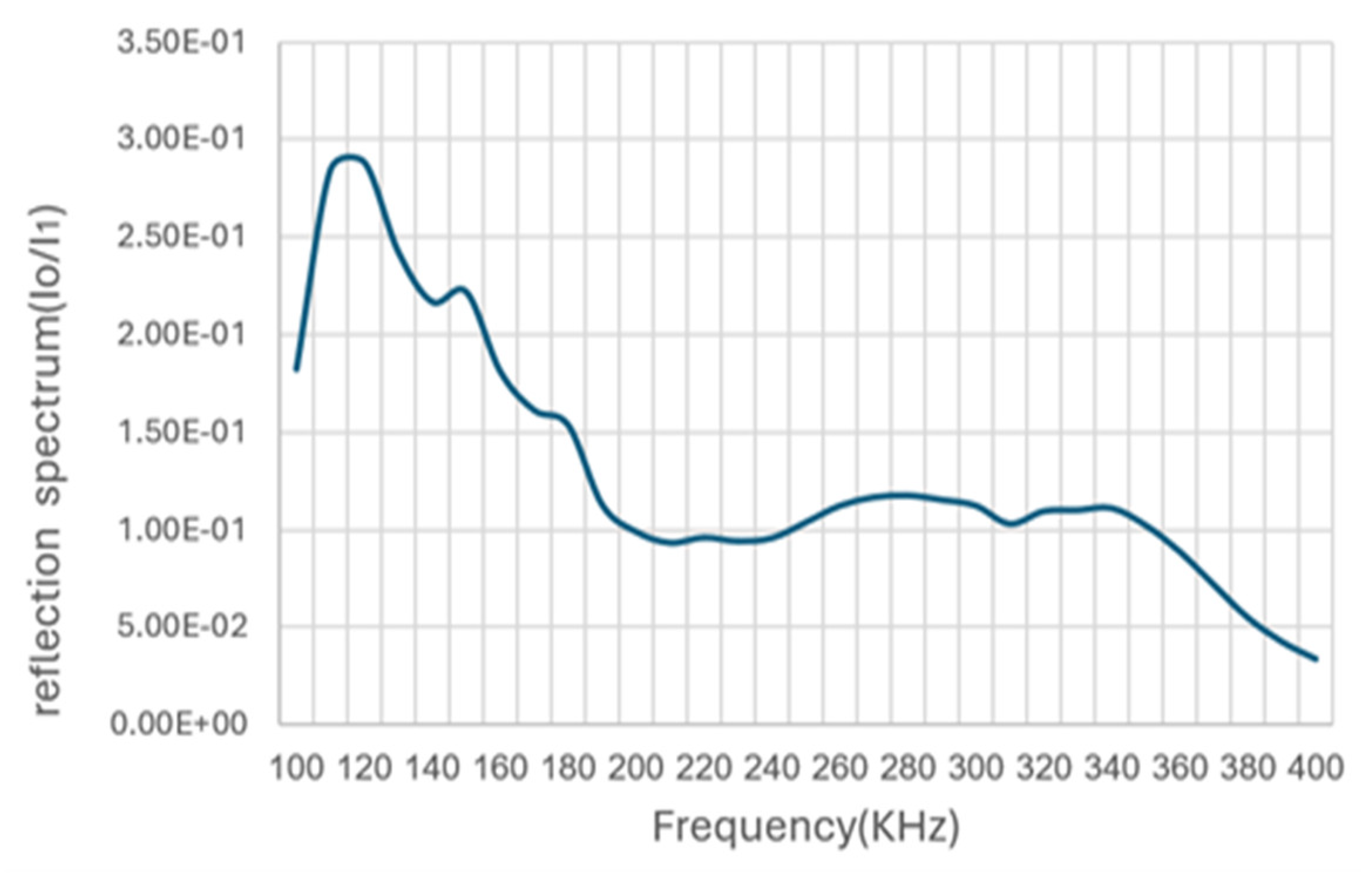
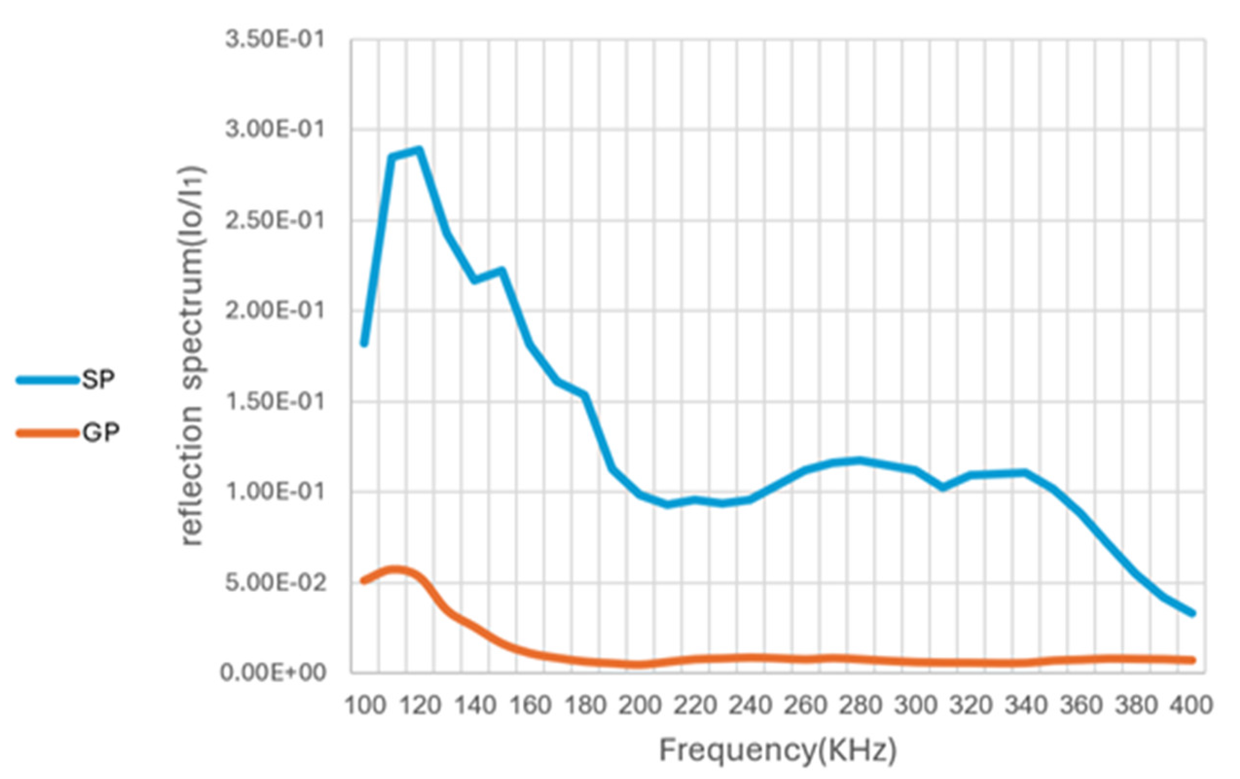
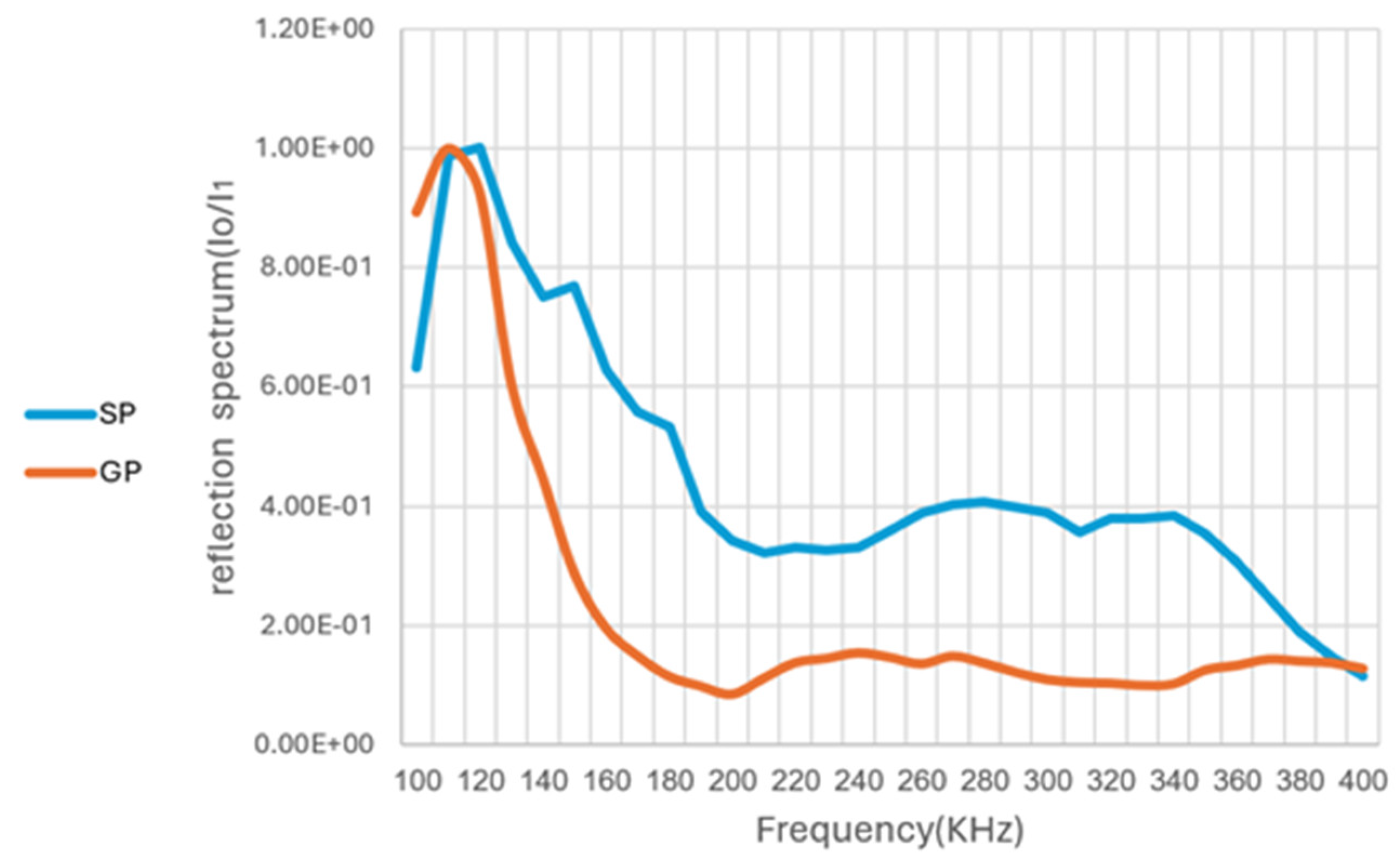
The results demonstrate a clear spectral distinction between SP and GP soils, confirming that frequency-dependent reflectance coefficients can serve as a reliable classification parameter. This validates the hypothesis that spectral acoustic signatures provide a finer-scale differentiation than traditional backscatter-based methods.

This differentiation highlights the potential of using acoustic spectral signatures as an alternative to traditional seabed classification methods. The findings suggest that the frequency-dependent behavior of acoustic waves interacting with sediments is influenced by grain size, grading characteristics, and microstructural differences, which are often overlooked in conventional acoustic seabed mapping techniques.

4.2. Comparison with Previous Studies

Existing seabed classification techniques have primarily relied on backscatter intensity analysis, which, being an integral phenomenon, often lacks the sensitivity required to distinguish between sediments with modest differences in grain size and different grading structures. While traditional methods are effective in broad classifications, they struggle with fine-scale discrimination due to overlapping acoustic responses in materials of similar density and composition.

A fundamental shift in approach is introduced in this study. Instead of relying on backscatter intensity, we analyze the coherent acoustic return spectrum—the outgoing to incoming energy ratio. This approach isolates the spectral response of the seabed alone, minimizing the influence of water column effects and isolating the impact of intrinsic factors on the reflection spectrum. Previous methods rely on backscatter intensity measurements, an integral quality that cannot adhere to subtle grain size, shape, and composition changes. The method presented here enables more precise classification, particularly in distinguishing between sediments that differ in grading and internal structure and more minor differences in grain size.

The observed spectral distinction between SP and GP supports the validity of this new approach. The results indicate that grading characteristics, pore water content, and particle arrangement significantly impact energy scatter, transmission, and reflection. These findings suggest that existing classification methods could be substantially improved by integrating spectral-based approaches to enhance their accuracy and reliability.

4.3. Physical Mechanisms Behind the Observed Spectral Differences

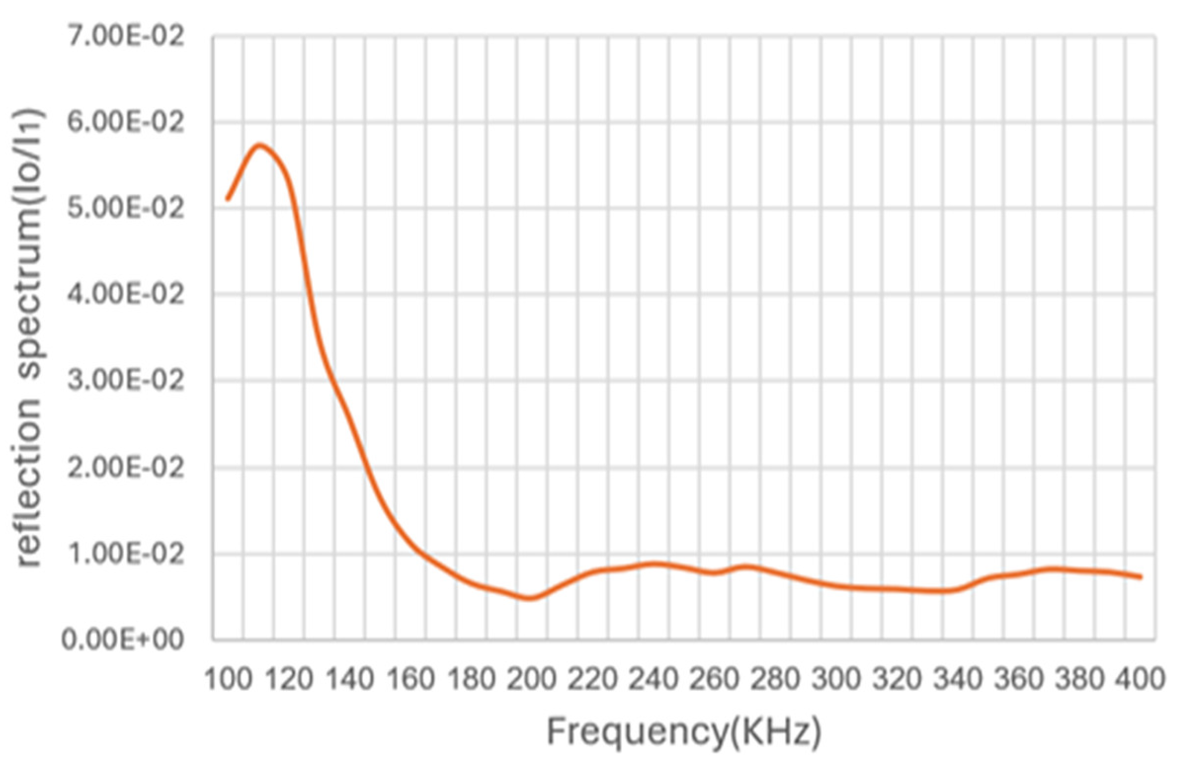
The results indicate that the higher return spectrum observed in SP (compared to GP) can be attributed to several physical mechanisms affecting energy absorption and scattering:

The differences in spectral reflectance can be attributed to combined impedance mismatch and microstructural scattering. SP soils exhibit a denser packing structure, leading to higher impedance contrast and greater reflection intensity. With their coarser grains and larger pore spaces, GP soils facilitate increased energy dissipation and scattering, resulting in a lower coherent reflection.

Grain size vs. wavelength ratio also significantly influences the spectrum’s shape. The average grain size of SP (~0.4 mm) is considerably smaller relative to the acoustic wavelengths (100–400 kHz). Hence, the classic theory of Snell’s law is more dominant, with a more substantial coherent part and a weaker backscatter. As expected, the coherent part is more significant for the lower range of frequencies (with a larger wavelength), as evidenced by the results. GP, with a coarser grain size (~5 mm) and, hence, a coarser relief concerning the wavelength, interacts differently with the acoustic wave, with a much more significant scattering of the acoustic waves leading to a much smaller coherent reflection. Also, here, we see an amplification of the coherent part for the lower frequencies; however, this is much less prominent than in the case of SP.

This study provides a clear physical basis for spectral-based seabed classification by identifying the dominant factors influencing spectral variation.

4.4. Advantages of the Proposed Approach

The proposed method is non-invasive by nature compared to physical sampling. Unlike sediment sampling, which requires physical retrieval and disturbs the marine environment, the proposed method is completely non-destructive and can be applied over large areas without ecological impact.

Compared to backscatter-based seabed classification methods, acoustic spectral analysis offers several key advantages:

Higher Resolution and Sensitivity: Differentiating soil types based on spectral characteristics rather than just intensity enables a finer-scale classification of seabed material.

The method is Independent of Water Column Effects: Traditional backscatter-based methods are significantly affected by variations in water properties, leading to inconsistencies. By isolating the energy entering and leaving the sediment, our approach eliminates water column distortions and directly assesses seabed properties.

Potential for Automation: The method can be integrated with machine learning algorithms for automated classification, reducing human interpretation errors, and increasing efficiency.

Real-Time Data Processing: Unlike traditional methods that require post-processing of sediment samples, this technique enables real-time seabed characterization, which is particularly beneficial for underwater construction, environmental monitoring, and geological surveys.

4.5. Limitations of the Study

While the results are promising, certain limitations should be acknowledged. Controlled Environment: This study was conducted in a controlled freshwater environment to isolate spectral effects. Future studies should investigate the method’s performance in open marine conditions with variable salinity, wave action, and biological activity.

This study focused on measurements taken at a fixed transducer angle. Future research should explore the effect of varying angles of incidence on the spectral return.

This study tested only two distinct soil types. To confirm the method’s robustness, further research should analyze a broader range of sediments, including mixed compositions and heterogeneous substrates. Potential Noise and Interference: In practical applications, biological activity, sediment resuspension, and underlying geological layers may introduce spectral variability. Refining signal processing techniques will be crucial for mitigating such effects.

4.6. Practical Applications

This study introduces a novel spectral classification framework for sediment differentiation, demonstrating that acoustic reflection coefficients provide a more refined alternative to backscatter intensity-based methods. This methodology sets the foundation for high-resolution, non-invasive seabed classification, which has potential applications in environmental monitoring, geotechnical engineering, and marine habitat assessment.

For example, seabed composition is critical for subsea construction, pipeline installations, and offshore wind farms in offshore engineering and infrastructure. The proposed method can aid in geotechnical assessments for these applications. In environmental monitoring, spectral acoustic analysis can be used to track sediment transport, erosion patterns, and pollution impacts in marine environments. For hydrographic surveys and geophysical exploration, the method offers a cost-effective and scalable seafloor geological and geophysical mapping solution.

5. Conclusions

5.1. Summary of Findings

This study provides compelling evidence that acoustic reflectance spectrum analysis can effectively distinguish between different soil types in an aquatic environment. The precise and repeatable spectral differences observed between missing graded sand (SP) and missing graded gravel (GP) suggest that grading characteristics and grain size play a significant role in shaping acoustic wave interactions. These findings reinforce the viability of using frequency-dependent acoustic responses for sediment classification, offering an alternative to traditional intensity-based acoustic approaches.

5.2. Contribution to Scientific Research

The research advances seabed classification techniques by demonstrating the feasibility of using spectral signatures for sediment differentiation. Unlike conventional methods, which rely heavily on backscatter intensity and empirical ground-truthing, the proposed approach provides a quantitative and reproducible means of classifying marine soils. This work lays the foundation for further exploration into spectral-based acoustic methods and their integration with advanced signal processing and AI-driven classification frameworks.

5.3. Future Research Directions

To further develop and refine this methodology, future studies should focus on:

• Expanding the Spectral Database: Establishing a comprehensive reference dataset of spectral signatures for different sediment types to facilitate machine learning-based classification models.
• Analyzing the Effect of Incidence Angle: Investigating how different transducer orientations influence spectral characteristics to improve robustness across diverse seabed geometries.
• Testing in Diverse Marine Environments: Conducting field studies in coastal and deep-sea environments to validate performance under real-world conditions.
• Machine Learning Integration: Developing AI-driven classification systems to automate spectral-based sediment identification and improve real-time processing capabilities.
• Hybrid Approaches: Combining coherent spectral analysis with traditional backscatter methods to develop an integrated multimodal classification framework.

Addressing these research areas could make acoustic spectral analysis a standardized, high-resolution, and real-time tool for seabed classification. The ability to characterize marine soils based on their unique spectral signatures represents a significant advancement in marine geotechnical science, opening new possibilities for environmental monitoring, offshore engineering, and aquatic habitat mapping.