Abstract
The Modified Ibarra–Medina–Krawinkler (ModIMK) model, based on phenomenology, is widely used by earthquake engineering researchers due to its fast computation and effectiveness in simulating the performance deterioration of structural components. In the past, the main study objects were reinforced concrete (RC) square columns. However, RC circular columns have seldom been studied, and their ModIMK model still needs to be developed. For this reason, we collected the pseudo-static test data of 80 circular columns and calibrated the model parameters of each component; through the regression method, empirical equations between the design parameters and the hysteretic model parameters were established, i.e., the ModIMK model was determined. Using the hysteretic model in this work, the hysteretic responses of eight circular columns were predicted and found to be well fitted to the test hysteretic responses, verifying the model’s accuracy. This work enabled a more comprehensive and accurate application of the ModIMK model in earthquake engineering studies involving RC circular columns.
1. Introduction
A performance-based earthquake engineering study needs a relatively reliable hysteretic model. The model must be able to capture the structural seismic responses in different damage states, especially from the severe damage stage to the collapse stage; the model is also required to accurately capture the behaviors of the components’ continuous deterioration in strength and stiffness under earthquake motions. The Ibarra–Medina–Krawinkler (IMK) model [1] and the Modified IMK (ModIMK) model [2], which are founded on the hysteretic energy dissipation principle, could fulfill both of the previous requirements very well.
The hysteretic models for reinforced concrete (RC) components can be divided into “mechanical” and “phenomenological” models [3,4,5]. The mechanical model needs to be based on the accurate determination of the material’s mechanical properties, i.e., it needs accurate constitutive laws of the material, and the typical mechanical model is the fiber model; it is often difficult to accurately describe the phenomena, such as concrete crushing and reinforcement slipping. The empirical phenomenological hysteretic model, however, can better describe these phenomena. The ModIMK model is based on phenomenology, which not only describes complex experimental phenomena but also speeds up the computation of structural analyses; therefore, it is recommended by the U.S. Code ASCE 41, which has led to the wide application of this model in earthquake engineering studies.
The hysteretic model of a component can be determined by calibrating its individual model parameters, while empirical prediction equations for the model parameters can be obtained through statistical analyses after the calibration of the existing pseudo-static tests [6,7]. In order to ascertain the IMK model of RC square columns, Haselton [8] established a database, calibrated the model parameters of each component, and created empirical equations for each IMK model parameter. For the purpose of developing the IMK model for asymmetric components, Lignos [9,10] modified it and obtained the ModIMK model; he collected RC and steel components, calibrated each ModIMK model parameter, and then obtained its prediction equation. By contrasting the corroded and non-corroded RC square columns, Dai [11] developed the corroded columns’ empirical equations for the ModIMK model. Huang [12] established a database, calibrated the ModIMK model’s cyclic deterioration parameters for all columns, and created empirical prediction equations.
The studies mentioned above are on RC square columns, while RC circular columns have seldom been studied. Liu [13] developed the ModIMK hysteretic model for corroded circular columns, but this model relies on the ModIMK model for uncorroded columns, which is still incomplete. Dai [14] created empirical prediction equations for some parameters of the ModIMK hysteretic model, but the equations for parameters and have not been established. Additionally, in a database of 76 components, the P-Δ effect pattern was incorrectly chosen for 27 components, leading to inaccurate calibration results for the model parameters. Therefore, the ModIMK hysteretic model for circular columns requires further improvement and development. We collected 80 sets of pseudo-static test data for RC circular columns and conducted a calibration and prediction study of the model parameters. The peak-orientated ModIMK model was adopted, and the OpenSees (3.3.0) software was utilized to numerically simulate the test curves of each column to calibrate the hysteretic model parameters. Then, a statistical regression was performed between the components’ design parameters and each model parameter, and empirical equations were established. The accuracy of these empirical prediction equations was verified through the analysis of eight columns in the database and out of the database.
2. Database
2.1. Collection of Test Data
Eighty RC columns from the Pacific Earthquake Engineering Research Center (PEER) structural performance database and published papers [15,16,17,18,19,20,21,22,23,24,25] were collected for this study, and the details of each component are listed in Table A1 and Table A2. Some of the following factors were considered in the collection of the test data: (1) the cross-section has to be circular; square and octagonal columns were not collected; (2) the forms of damage were flexural and flexural-shear; those with a shear damage form were not collected; (3) according to the type of construction and loading boundary conditions, the method of reference [25] was used to convert all the test data uniformly into the force–displacement form of cantilevered columns; (4) the method of reference [25] was used to differentiate the type of P-Δ effect correction, and those with an unclear type of P-Δ effect were not collected; after considering the P-Δ effect, the force–displacement form of the test data was converted into the form of moment rotation.
2.2. Design Parameters and Their Range of Values
The physical significance and the range of values of the design parameters are shown in Table 1 and Table 2. Based on the analyses in references [8,11,26], the variables that have a more significant effect on the model parameters were selected as the design parameters. Table 2 lists the range of values of the main design parameters of the components; the axial compression ratio ranges from −0.01 to 0.419, so it can be seen that the empirical prediction equations in this work are more suitable for low and medium axial pressures.

Table 1.
Design parameters of circular components.
Table 2.
Value ranges of design parameters.
3. The ModIMK Model and Parameters’ Calibration
3.1. The ModIMK Hysteretic Model
The ModIMK model consists of two parts, the backbone curve and the hysteresis rule, and the backbone curve of the model is shown in Figure 1. The ModIMK hysteretic model has a critical difference compared with other models; its backbone curve is not acquired by linking the peak moment point of every hysteresis loop directly, but it is obtained based on the monotonic loading curve (see Figure 1). The backbone curve connecting the peak moment points varies greatly depending on the loading history, whereas the monotonic loading curve is stable.
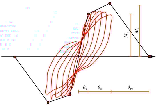
Figure 1.
Backbone curve of ModIMK model.
Because most test groups did not have monotonically loaded components, the backbone curve is generally approximated by calibrating the hysteresis curve.
The ModIMK hysteresis model has three types: bilinear, peak-orientated, and pinching; the circular columns collected in this work are more compatible with the peak-orientated type. The main model parameters are listed in Table 3, and other ones can be viewed on the official website of OpenSees.
Table 3.
Meaning of model parameters.
3.2. The Model Parameters’ Calibration
The backbone curve reflects the component’s monotonic loading process, so the model parameters cannot be obtained directly by analyzing the test hysteresis curve. The component’s deterioration behavior is determined by the energy dissipation throughout the loading process, and the deterioration coefficients cannot be obtained through simple calculations. Only by the numerical simulation of the test process and by analyzing the fitting situation between the test curve and the simulation curve can the model parameters of the component be finally determined. Therefore, a finite element model needs to be created for each component for the numerical analysis.
The peak-orientated ModIMK model is suitable for RC circular columns where flexural deformation is dominant. According to the analysis of reference [26], six model parameters, i.e., , can determine the hysteretic model of a component.
According to reference [26], the analytical model was developed, and the model parameters were calibrated using the OpenSees platform. Due to the fact that the plastic hinge can only appear after a component yields, the analytical model differs from the real test, and in order to simulate this more accurately, the analytical model has to be stiffness-corrected [27,28,29].
The model parameters were calibrated in the positive and negative loading directions, and then their average values were obtained, which are listed in Table A1. The empirical prediction equations were created on the basis of the statistical regression of the average values.
4. Empirical Equations for Model Parameters
4.1. Regression Analysis Method for Model Parameters
The empirical prediction equations linking the design parameters and the calibrated model parameters were developed through the regression method. The regression process is as follows:
- (1)
- The form of the prediction equations
According to reference [10], each empirical prediction equation’s form was selected as follows:
where represent a model parameter, represents the component design parameters, and represents the regression parameters. The 15 design parameters are listed in Table 1. Since some components do not have an axial pressure, in order to carry out the regression analyses when taking logarithms, (v + 1) is used as the input parameter for the axial pressure ratio.
- (2)
- The linear regression analysis method
After taking natural logarithms on both sides of Equation (1) simultaneously, Equation (2) was obtained:
The natural logarithm was taken for the calibrated model parameters and the design parameters of each component. Then, linear regression was carried out to determine Equation (2). The selected design parameters require a t-test significance level of less than 0.05. In order to control the multicollinearity of the selected design parameters, the VIF (Variance Inflation Factor) of each parameter is required to be less than 10.
- (3)
- The establishment of the empirical prediction equations
The regression equation for each model parameter can be obtained by taking the natural constant e as the bottom index for both sides of Equation (2).
4.2. Empirical Equations
- (1)
- The empirical prediction equations
Through a regression analysis, the empirical prediction equations were obtained as follows:
Most of the circular columns in the database were not loaded to softening stage, and could not be measured, so the regression method was not used to obtain the empirical equation for . According to reference [8], it has been shown that there is an empirical relationship between the initial stiffness and the softening stiffness, i.e., , and after determining , the estimation Equation (8) can be obtained. In addition, according to the test results of 15 adequately loaded components, 0.1 is set as the upper limit value of [8]. The larger value of is generally due to the fact that the loading is not sufficiently adequate, and the deterioration in the components is not yet apparent.
- (2)
- Evaluation of the prediction equations
The coefficients of determination (R2) of the regression equations for model parameters are 0.98, 0.65, 0.54, and 0.50, respectively, which indicates that the regression equations are well fitted; the coefficient of determination of is 0.36, which indicates that this parameter has a poorer correlation with the design parameters.
For each model parameter of each component, the ratio between the calibrated and predicted values was calculated. The statistics of this ratio are presented in Table 4; , , and are the mean, median, and standard deviation, respectively.
Table 4.
Statistical information for ratios of calibrated to predicted model parameters.
Table 4 shows that the ratios’ mean values corresponding to the model parameters are 1.01, 1.02, 1.02, 1.09, and 1.13, and the median values are 0.99, 1.01, 1.02, 0.99, and 1.0, respectively, which indicates that the prediction equations can predict the hysteretic model parameters relatively well. The standard deviations of the ratios corresponding to the model parameters are 0.18, 0.22, 0.11, 0.44, and 0.57, respectively, so it can be seen that the prediction accuracies of are high, and the dispersion is small. In contrast, the dispersion of is relatively large.
It should be noted that the statistical data of is from reference [8], and its corresponding mean and median values are 1.2 and 1.0, while the logarithmic standard deviation is 0.72. Since, after the peak point of the backbone curve, the cracking of the components, the slipping of the reinforcement, and the shear deformation are more serious, the standard deviation and dispersion are relatively large, and the accuracy of the prediction result of will be smaller than that of the other parameters.
The model parameters of the 80 columns in the database were predicted using the aforementioned empirical prediction equations. Figure 2 illustrates the comparison between the predicted and calibrated model parameters, showing that the two are generally well matched.
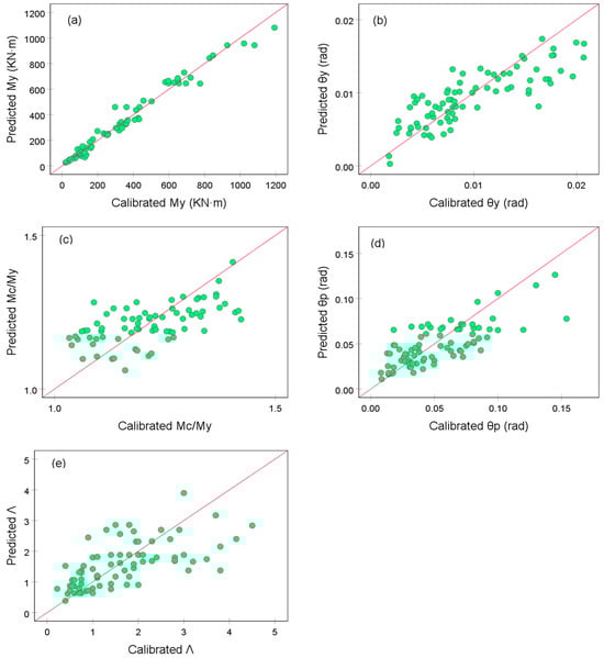
Figure 2.
Comparison of calibrated and predicted parameters. (a) ; (b) ; (c) ; (d) ; and (e) .
Generally speaking, the hysteretic model parameters can be reliably predicted using the proposed empirical prediction equations.
5. Validation of the Empirical Prediction Equations
In order to validate the accuracy of the proposed empirical equations, eight components, four inside and four outside the database, were selected for analysis. The predicted model parameters of the components were derived using the empirical prediction equations, and the predicted hysteretic curves were obtained through a numerical simulation; then, the test hysteretic curves and the predicted hysteretic curves were compared.
5.1. Validation of the Components in the Database
Based on the collected data information, the axial pressure ratios were categorized into three cases: , low axial pressure ratio; , medium axial pressure ratio; and , higher axial pressure ratio. In each range of axial pressure ratios, representative components were randomly selected for validation. The four components numbered 298, 360, 384, and 392 in the database have axial pressure ratios of 0.39, 0.307, 0.419, and 0.12, respectively. Their design parameters are presented in Table A2, and their predicted model parameters are listed in Table 5. Figure 3 shows the predicted hysteresis curves and the test hysteresis curves. It is clear that the hysteresis behavior of each test can be predicted well, and the yield moment, yield rotation, hardening stiffness, and capping moment are all well fitted; through the last hysteresis loop of 298, it is also evident that the model in this work is quite accurate in predicting the softening stiffness after the capping point.
Table 5.
Predicted model parameters of intra-database columns.
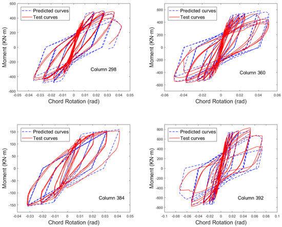
Figure 3.
Predicted and test curves of intra-database columns.
Through the hysteresis curves of the three components of 298, 360, and 392, it can be found that the model in this work has an outstanding capability for capturing the performance deterioration in the components.
The analyses of the above four components in the database prove that the model proposed in this work can predict the hysteretic responses well.
5.2. Applications Outside the Database
Since relatively few components with higher axial compression ratios were collected, the equations in this work are more applicable to the case of medium and low axial compression ratios. Four components, Wong-No.1, NiST-N5, Vu-NH3, and Calderone-328, were selected to apply the hysteretic model in this work for a hysteretic response analysis [25]. Their design parameters are listed in Table 6, while their predicted model parameters are listed in Table 7. The axial pressure ratios of the four components are 0.19, 0.20, 0.15, and 0.091, which represent the medium or low axial pressure ratios, respectively. From Figure 4, it is evident that the presented hysteretic model can predict the hysteretic responses well. Similar to the analysis within the database, the model parameters are predicted relatively accurately. The analyses of the last few hysteretic loops of the hysteresis curves shows that the deterioration in the components can be simulated well.
Table 6.
Design parameters of 4 columns for applied analyses.
Table 7.
Predicted parameters.
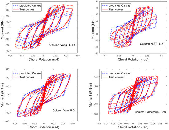
Figure 4.
Predicted and test curves of 4 columns for applied analyses.
The analyses of the above four components shows that the model proposed in this work is also very applicable in applications outside the database.
6. Conclusions
The ModIMK hysteretic model for RC circular columns was created by a regression method, and the summaries and conclusions are shown below:
- (1)
- A database of 80 RC circular columns undergoing flexural or flexural-shear damage had been established, containing 15 design parameters and the calibrated ModIMK model parameters. For further research on various characteristics of RC circular columns, the database is an invaluable resource.
- (2)
- The empirical prediction equations for the hysteretic model parameters based on the design parameters were established, i.e., the ModIMK model was determined. The predicted and test hysteretic curves were compared to confirm the proposed model can predict hysteretic behavior accurately. This work enabled a more comprehensive and accurate application of the ModIMK model in earthquake engineering studies involving RC circular columns.
Of course, due to the limited numbers of the database, there exists a specific range of applicability of the design parameters; therefore, when using the prediction equations, taking note of the design parameters’ values is essential. In the future, with the continuous increase in test data, the proposed ModIMK model will be continuously improved to gradually increase its applicability and accuracy.
Author Contributions
Conceptualization, J.L. (Junqi Lin) and J.L. (Jinlong Liu); methodology, H.L.; software, H.L.; validation, H.L., J.L. (Junqi Lin) and J.L. (Jinlong Liu); formal analysis, H.L.; investigation, H.L.; resources, J.L. (Junqi Lin); data curation, H.L.; writing—original draft preparation, H.L.; writing—review and editing, H.L.; visualization, H.L.; supervision, J.L. (Junqi Lin); project administration, J.L. (Junqi Lin); funding acquisition, J.L. (Junqi Lin) and J.L. (Jinlong Liu). All authors have read and agreed to the published version of the manuscript.
Funding
This research was funded by Scientific Research Fund of Institute of Engineering Mechanics, China Earthquake Administration (2024B21).
Data Availability Statement
The original contributions presented in the study are included in the article, further inquiries can be directed to the corresponding author.
Conflicts of Interest
The authors declare no conflict of interest.
Appendix A
Table A1.
Circular columns’ calibrated model parameters.
Table A1.
Circular columns’ calibrated model parameters.
| No. | Reference | Component No. | ||||||
|---|---|---|---|---|---|---|---|---|
| 1 | Ma [15] | c0-15 | 63.46 | 0.0085 | 1.260 | 0.0500 | — | 3.10 |
| 2 | c0-25 | 71.41 | 0.0094 | 1.254 | 0.0496 | 0.0760 | 3.80 | |
| 3 | c0-40 | 85.00 | 0.0065 | 1.173 | 0.0410 | — | 1.70 | |
| 4 | Zhu [16] | C0 | 79.20 | 0.0092 | 1.094 | 0.0130 | 0.0938 | 2.00 |
| 5 | Zhou [17] | LL | 36.13 | 0.0111 | 1.701 | 0.0545 | — | 1.95 |
| 6 | MM | 73.91 | 0.0176 | 1.532 | 0.0935 | — | 2.70 | |
| 7 | MH | 106.51 | 0.0218 | 1.463 | 0.0810 | — | 4.15 | |
| 8 | Li [18,19] | C80 | 96.21 | 0.0119 | 1.183 | 0.0307 | — | 0.75 |
| 9 | C140 | 86.40 | 0.0077 | 1.213 | 0.0085 | — | 0.45 | |
| 10 | Feng [20,21] | L0-N3-C0 | 104.44 | 0.0096 | 1.409 | 0.0225 | — | 0.90 |
| 11 | Aquino [22] | no.6 | 297.17 | 0.0090 | 1.269 | 0.0412 | 0.1134 | 1.15 |
| 12 | Lao [23] | C-0-L0-N02 | 127.18 | 0.0144 | 1.106 | 0.0240 | — | 0.40 |
| 13 | C-0-L0-N04 | 135.75 | 0.0114 | 1.067 | 0.0180 | — | 0.80 | |
| 14 | Xie [24] | BW-1 | 44.90 | 0.0101 | 1.176 | 0.0286 | — | 0.75 |
| 15 | PEER [25] | 267 | 233.50 | 0.0213 | 1.087 | 0.0260 | — | 0.70 |
| 16 | 268 | 172.50 | 0.0079 | 1.052 | 0.0380 | — | 2.00 | |
| 17 | 269 | 258.00 | 0.0236 | 1.039 | 0.0150 | — | 0.50 | |
| 18 | 271 | 254.00 | 0.0225 | 1.080 | 0.0180 | — | 0.55 | |
| 19 | 274 | 358.00 | 0.0195 | 1.226 | 0.0320 | 0.0946 | 0.75 | |
| 20 | 275 | 355.00 | 0.0175 | 1.339 | 0.0550 | — | 1.90 | |
| 21 | 276 | 360.50 | 0.0203 | 1.163 | 0.0360 | — | 0.60 | |
| 22 | 277 | 323.00 | 0.0193 | 1.033 | 0.0135 | — | 0.22 | |
| 23 | 278 | 320.00 | 0.0210 | 1.074 | 0.0370 | — | 1.10 | |
| 24 | 279 | 337.00 | 0.0169 | 1.267 | 0.0630 | — | 0.70 | |
| 25 | 280 | 245.00 | 0.0120 | 1.219 | 0.0340 | 0.1873 | 0.60 | |
| 26 | 281 | 156.00 | 0.0078 | 1.257 | 0.0480 | — | 1.40 | |
| 27 | 289 | 256.00 | 0.0118 | 1.118 | 0.0300 | — | 0.85 | |
| 28 | 290 | 254.50 | 0.0126 | 1.189 | 0.0725 | — | 1.00 | |
| 29 | 297 | 361.50 | 0.0067 | 1.109 | 0.0080 | 0.0536 | 0.50 | |
| 30 | 298 | 434.00 | 0.0095 | 1.205 | 0.0270 | 0.0505 | 1.10 | |
| 31 | 303 | 19.65 | 0.0247 | 1.047 | 0.0395 | 0.1445 | 1.90 | |
| 32 | 304 | 22.40 | 0.0189 | 1.222 | 0.0700 | — | 2.10 | |
| 33 | 305 | 23.50 | 0.0182 | 1.061 | 0.0650 | — | 3.00 | |
| 34 | 308 | 47.20 | 0.0120 | 1.331 | 0.1540 | — | 1.60 | |
| 35 | 309 | 56.00 | 0.0115 | 1.291 | 0.1200 | — | 1.40 | |
| 36 | 310 | 41.60 | 0.0083 | 1.594 | 0.0700 | — | 2.80 | |
| 37 | 311 | 47.00 | 0.0103 | 1.244 | 0.0960 | — | 1.80 | |
| 38 | 313 | 48.20 | 0.0115 | 1.187 | 0.1000 | — | 2.30 | |
| 39 | 346 | 100.00 | 0.0139 | 1.294 | 0.0470 | — | 2.40 | |
| 40 | 347 | 98.50 | 0.0114 | 1.159 | 0.0320 | — | 5.30 | |
| 41 | 349 | 109.50 | 0.0162 | 1.229 | 0.0400 | — | 2.80 | |
| 42 | 350 | 101.00 | 0.0122 | 1.190 | 0.0565 | — | 1.00 | |
| 43 | 357 | 332.00 | 0.0059 | 1.265 | 0.0315 | — | 0.90 | |
| 44 | 358 | 456.50 | 0.0058 | 1.266 | 0.0140 | 0.0320 | 0.40 | |
| 45 | 359 | 1192.50 | 0.0160 | 1.186 | 0.0800 | — | 3.80 | |
| 46 | 360 | 502.50 | 0.0122 | 1.326 | 0.0420 | — | 1.10 | |
| 47 | 361 | 198.50 | 0.0082 | 1.366 | 0.0180 | — | 1.10 | |
| 48 | 363 | 775.00 | 0.0240 | 1.372 | 0.0850 | — | 1.60 | |
| 49 | 364 | 302.50 | 0.0154 | 1.386 | 0.0750 | — | 1.75 | |
| 50 | 365 | 827.50 | 0.0201 | 1.403 | 0.0850 | — | 3.50 | |
| 51 | 366 | 579.00 | 0.0247 | 1.192 | 0.0765 | 0.3986 | 2.10 | |
| 52 | 367 | 600.00 | 0.0207 | 1.144 | 0.0380 | 0.0574 | 1.40 | |
| 53 | 368 | 629.00 | 0.0218 | 1.157 | 0.0810 | — | 3.20 | |
| 54 | 369 | 655.50 | 0.0107 | 1.133 | 0.0710 | — | 1.10 | |
| 55 | 370 | 695.00 | 0.0194 | 1.096 | 0.0840 | — | 1.60 | |
| 56 | 371 | 597.00 | 0.0215 | 1.107 | 0.1000 | — | 1.80 | |
| 57 | 372 | 415.00 | 0.0097 | 1.089 | 0.0450 | — | 2.00 | |
| 58 | 373 | 1021.50 | 0.0147 | 1.311 | 0.0725 | — | 1.00 | |
| 59 | 375 | 927.50 | 0.0187 | 1.214 | 0.1300 | — | 4.50 | |
| 60 | 376 | 1080.00 | 0.0216 | 1.215 | 0.1450 | — | 3.70 | |
| 61 | 377 | 651.00 | 0.0142 | 1.422 | 0.0710 | — | 1.80 | |
| 62 | 378 | 649.00 | 0.0153 | 1.484 | 0.0630 | — | 1.50 | |
| 63 | 379 | 721.50 | 0.0129 | 1.416 | 0.0915 | — | 1.90 | |
| 64 | 380 | 121.00 | 0.0164 | 1.276 | 0.0810 | — | 7.80 | |
| 65 | 381 | 112.00 | 0.0127 | 1.321 | 0.0630 | — | 6.00 | |
| 66 | 382 | 135.50 | 0.0085 | 1.322 | 0.0600 | — | 2.50 | |
| 67 | 383 | 126.00 | 0.0110 | 1.304 | 0.0190 | 0.0475 | 1.50 | |
| 68 | 384 | 123.50 | 0.0100 | 1.335 | 0.0270 | — | 2.30 | |
| 69 | 385 | 125.50 | 0.0173 | 1.366 | 0.0800 | — | 2.90 | |
| 70 | 386 | 136.50 | 0.0121 | 1.291 | 0.0350 | — | 1.30 | |
| 71 | 387 | 161.00 | 0.0129 | 1.338 | 0.0550 | — | 3.00 | |
| 72 | 388 | 427.50 | 0.0117 | 1.096 | 0.0165 | — | 0.60 | |
| 73 | 389 | 432.00 | 0.0079 | 1.064 | 0.0140 | — | 0.75 | |
| 74 | 390 | 407.50 | 0.0086 | 1.130 | 0.0335 | 0.0269 | 1.00 | |
| 75 | 391 | 368.00 | 0.0067 | 1.134 | 0.0175 | — | 0.70 | |
| 76 | 392 | 685.00 | 0.0116 | 1.374 | 0.0680 | 0.4156 | 1.10 | |
| 77 | 393 | 596.50 | 0.0123 | 1.456 | 0.0865 | — | 0.75 | |
| 78 | 394 | 847.50 | 0.0116 | 1.160 | 0.0300 | — | 0.55 | |
| 79 | 408 | 115.50 | 0.0108 | 1.228 | 0.0435 | — | 2.80 | |
| 80 | 412 | 165.50 | 0.0099 | 1.186 | 0.0330 | — | 1.40 |
Note: ‘—’ in the θpc column means ‘no data’, which denotes that θpc cannot be calibrated.
Table A2.
Design parameters of components.
Table A2.
Design parameters of components.
| No. | Component No. | P-Δ Type | d | c | + 1 | s/d | |||||||||||
|---|---|---|---|---|---|---|---|---|---|---|---|---|---|---|---|---|---|
| 1 | c0-15 | shear | 260 | 30 | 25.92 | 16.0 | 0.0227 | 3.15 | 1.150 | 12.074 | 6.250 | 0.526 | 373.2 | 572.3 | 8.0 | 0.0100 | 327.0 |
| 2 | c0-25 | shear | 260 | 30 | 25.92 | 16.0 | 0.0227 | 3.15 | 1.250 | 12.074 | 6.250 | 0.519 | 373.2 | 572.3 | 8.0 | 0.0100 | 327.0 |
| 3 | c0-40 | shear | 260 | 30 | 25.92 | 16.0 | 0.0227 | 3.15 | 1.400 | 12.074 | 6.250 | 0.578 | 373.2 | 572.3 | 8.0 | 0.0100 | 327.0 |
| 4 | C0 | shear | 300 | 30 | 24.34 | 16.0 | 0.0171 | 3.67 | 1.200 | 8.840 | 4.688 | 0.389 | 355.6 | 538.3 | 8.0 | 0.0112 | 230.7 |
| 5 | LL | shear | 240 | 20 | 32.00 | 12.0 | 0.0150 | 5.83 | 1.057 | 8.333 | 4.167 | 0.184 | 400.0 | 540.0 | 6.0 | 0.0113 | 400.0 |
| 6 | MM | shear | 240 | 20 | 32.00 | 16.0 | 0.0355 | 7.50 | 1.071 | 6.250 | 3.125 | 0.288 | 400.0 | 540.0 | 6.0 | 0.0113 | 400.0 |
| 7 | MH | shear | 240 | 20 | 32.00 | 20.0 | 0.0563 | 7.50 | 1.071 | 5.000 | 2.500 | 0.412 | 400.0 | 540.0 | 6.0 | 0.0113 | 400.0 |
| 8 | C80 | shear | 300 | 30 | 26.48 | 14.0 | 0.0218 | 4.67 | 1.147 | 16.840 | 8.571 | 0.475 | 386.0 | 628.0 | 6.0 | 0.0039 | 367.0 |
| 9 | C140 | shear | 300 | 30 | 26.48 | 14.0 | 0.0218 | 4.67 | 1.410 | 29.470 | 15.000 | 0.485 | 386.0 | 628.0 | 6.0 | 0.0022 | 367.0 |
| 10 | L0-N3-C0 | shear | 300 | 30 | 35.44 | 16.0 | 0.0171 | 5.00 | 1.300 | 7.632 | 3.125 | 0.203 | 596.4 | 734.9 | 8.0 | 0.0167 | 404.9 |
| 11 | no.6 | shear | 500 | 25 | 32.00 | 25.4 | 0.0310 | 4.20 | 1.000 | 16.137 | 7.874 | 0.457 | 420.0 | 620.0 | 9.5 | 0.0031 | 420.0 |
| 12 | C-0-L0-N02 | shear | 250 | 25 | 26.16 | 16.0 | 0.0246 | 4.54 | 1.200 | 13.376 | 6.250 | 0.679 | 458.0 | 620.0 | 8.0 | 0.0100 | 454.0 |
| 13 | C-0-L0-N04 | shear | 250 | 25 | 26.16 | 16.0 | 0.0246 | 4.54 | 1.400 | 13.376 | 6.250 | 0.652 | 458.0 | 620.0 | 8.0 | 0.0100 | 454.0 |
| 14 | BW-1 | shear | 240 | 25 | 34.24 | 10.0 | 0.0174 | 5.83 | 1.100 | 22.334 | 10.000 | 0.237 | 498.8 | 693.6 | 8.0 | 0.0106 | 358.6 |
| 15 | 267 | shear | 400 | 18 | 37.50 | 16.0 | 0.0320 | 2.00 | 1.000 | 7.830 | 3.750 | 1.405 | 436.0 | 674.0 | 6.0 | 0.0051 | 328.0 |
| 16 | 268 | shear | 400 | 18 | 37.20 | 16.0 | 0.0320 | 2.00 | 1.000 | 6.452 | 3.750 | 0.950 | 296.0 | 457.0 | 6.0 | 0.0051 | 328.0 |
| 17 | 269 | shear | 400 | 18 | 36.00 | 16.0 | 0.0320 | 2.50 | 1.000 | 7.830 | 3.750 | 1.055 | 436.0 | 674.0 | 6.0 | 0.0051 | 328.0 |
| 18 | 271 | shear | 400 | 18 | 31.10 | 16.0 | 0.0320 | 2.00 | 1.000 | 5.220 | 2.500 | 1.223 | 436.0 | 674.0 | 6.0 | 0.0076 | 328.0 |
| 19 | 274 | shear | 400 | 18 | 28.70 | 16.0 | 0.0320 | 2.00 | 1.200 | 3.969 | 1.875 | 0.937 | 448.0 | 693.0 | 6.0 | 0.0102 | 372.0 |
| 20 | 275 | shear | 400 | 18 | 29.90 | 16.0 | 0.0320 | 2.50 | 1.200 | 3.969 | 1.875 | 0.924 | 448.0 | 693.0 | 6.0 | 0.0102 | 372.0 |
| 21 | 276 | shear | 400 | 21 | 31.20 | 16.0 | 0.0320 | 2.00 | 1.200 | 15.875 | 7.500 | 1.022 | 448.0 | 693.0 | 12.0 | 0.0102 | 332.0 |
| 22 | 277 | shear | 400 | 18 | 29.90 | 16.0 | 0.0320 | 2.00 | 1.200 | 7.937 | 3.750 | 1.184 | 448.0 | 693.0 | 6.0 | 0.0051 | 372.0 |
| 23 | 278 | shear | 400 | 18 | 28.60 | 16.0 | 0.0320 | 1.50 | 1.100 | 3.915 | 1.875 | 1.463 | 436.0 | 674.0 | 6.0 | 0.0102 | 328.0 |
| 24 | 279 | shear | 400 | 18 | 36.20 | 16.0 | 0.0320 | 2.00 | 1.100 | 3.915 | 1.875 | 1.045 | 436.0 | 679.0 | 6.0 | 0.0102 | 326.0 |
| 25 | 280 | shear | 400 | 18 | 33.70 | 24.0 | 0.0324 | 2.00 | 1.000 | 5.148 | 2.500 | 1.352 | 424.0 | 671.0 | 6.0 | 0.0051 | 326.0 |
| 26 | 281 | shear | 400 | 18 | 34.80 | 16.0 | 0.0192 | 2.00 | 1.000 | 7.830 | 3.750 | 0.932 | 436.0 | 679.0 | 6.0 | 0.0051 | 326.0 |
| 27 | 289 | shear | 400 | 21 | 32.30 | 16.0 | 0.0320 | 2.00 | 1.000 | 20.881 | 10.000 | 1.178 | 436.0 | 679.0 | 12.0 | 0.0076 | 332.0 |
| 28 | 290 | shear | 400 | 20 | 33.10 | 16.0 | 0.0320 | 2.00 | 1.000 | 14.355 | 6.875 | 1.265 | 436.0 | 679.0 | 10.0 | 0.0077 | 310.0 |
| 29 | 297 | shear | 400 | 18 | 37.00 | 16.0 | 0.0320 | 2.00 | 1.390 | 8.854 | 4.063 | 0.809 | 475.0 | 625.0 | 6.0 | 0.0047 | 340.0 |
| 30 | 298 | shear | 400 | 20 | 37.00 | 16.0 | 0.0320 | 2.00 | 1.390 | 8.173 | 3.750 | 0.962 | 475.0 | 625.0 | 10.0 | 0.0142 | 300.0 |
| 31 | 303 | Feff | 152 | 10.2 | 34.50 | 12.7 | 0.0558 | 7.50 | 1.241 | 3.667 | 1.732 | 0.228 | 448.0 | 679.6 | 3.7 | 0.0145 | 620.0 |
| 32 | 304 | Feff | 152 | 10.2 | 34.50 | 12.7 | 0.0558 | 3.75 | 1.241 | 3.667 | 1.732 | 0.448 | 448.0 | 679.6 | 3.7 | 0.0145 | 620.0 |
| 33 | 305 | Feff | 152 | 10.2 | 34.50 | 12.7 | 0.0558 | 3.75 | 1.351 | 3.667 | 1.732 | 0.475 | 448.0 | 679.6 | 3.7 | 0.0145 | 620.0 |
| 34 | 308 | shear | 250 | 9.9 | 24.10 | 7.0 | 0.0196 | 3.00 | 1.101 | 2.715 | 1.286 | 0.308 | 446.0 | 676.6 | 3.1 | 0.0141 | 441.0 |
| 35 | 309 | shear | 250 | 9.9 | 23.10 | 7.0 | 0.0196 | 3.00 | 1.211 | 2.715 | 1.286 | 0.364 | 446.0 | 676.6 | 3.1 | 0.0141 | 441.0 |
| 36 | 310 | shear | 250 | 9.7 | 25.40 | 7.0 | 0.0196 | 6.00 | 1.096 | 4.224 | 2.000 | 0.220 | 446.0 | 676.6 | 2.7 | 0.0068 | 476.0 |
| 37 | 311 | shear | 250 | 9.9 | 24.40 | 7.0 | 0.0196 | 3.00 | 1.100 | 2.715 | 1.286 | 0.322 | 446.0 | 676.6 | 3.1 | 0.0141 | 441.0 |
| 38 | 313 | shear | 250 | 9.7 | 23.30 | 7.0 | 0.0196 | 6.00 | 1.105 | 4.224 | 2.000 | 0.619 | 446.0 | 676.6 | 2.7 | 0.0068 | 476.0 |
| 39 | 346 | shear | 305 | 14.5 | 29.00 | 9.5 | 0.0204 | 4.50 | 1.094 | 4.233 | 2.000 | 0.323 | 448.0 | 690.0 | 4.0 | 0.0094 | 434.0 |
| 40 | 347 | shear | 305 | 14.5 | 35.50 | 9.5 | 0.0204 | 4.50 | 1.086 | 4.233 | 2.000 | 0.307 | 448.0 | 690.0 | 4.0 | 0.0094 | 434.0 |
| 41 | 349 | shear | 305 | 14.5 | 35.50 | 9.5 | 0.0204 | 4.50 | 1.086 | 4.233 | 2.000 | 0.341 | 448.0 | 690.0 | 4.0 | 0.0094 | 434.0 |
| 42 | 350 | shear | 305 | 14.5 | 35.50 | 9.5 | 0.0204 | 4.50 | 1.094 | 4.233 | 2.000 | 0.330 | 448.0 | 690.0 | 4.0 | 0.0094 | 434.0 |
| 43 | 357 | Feff | 610 | 15.9 | 30.00 | 12.7 | 0.0052 | 1.50 | 1.057 | 12.897 | 6.000 | 0.164 | 462.0 | 700.9 | 6.4 | 0.0028 | 361.0 |
| 44 | 358 | Feff | 610 | 15.9 | 30.00 | 12.7 | 0.0104 | 1.50 | 1.057 | 21.494 | 10.000 | 0.187 | 462.0 | 700.9 | 6.4 | 0.0017 | 361.0 |
| 45 | 359 | Feff | 610 | 27.8 | 41.10 | 22.2 | 0.0266 | 6.00 | 1.148 | 5.477 | 2.568 | 0.076 | 455.0 | 746.0 | 9.5 | 0.0089 | 414.0 |
| 46 | 360 | Feff | 457 | 24.8 | 38.30 | 15.9 | 0.0241 | 1.99 | 1.307 | 7.802 | 3.774 | 0.672 | 427.5 | 648.5 | 9.5 | 0.0114 | 430.2 |
| 47 | 361 | Feff | 457 | 24.8 | 39.20 | 15.9 | 0.0241 | 1.99 | 0.901 | 7.802 | 3.774 | 0.519 | 427.5 | 648.5 | 9.5 | 0.0114 | 430.2 |
| 48 | 363 | Feff | 457 | 26.4 | 35.00 | 19.0 | 0.0521 | 1.99 | 1.148 | 5.125 | 2.368 | 0.716 | 468.2 | 710.3 | 12.7 | 0.0270 | 434.4 |
| 49 | 364 | Feff | 457 | 24.8 | 35.20 | 15.9 | 0.0241 | 1.99 | 0.915 | 11.335 | 5.031 | 0.875 | 507.5 | 769.9 | 9.5 | 0.0085 | 448.2 |
| 50 | 365 | Feff | 457 | 26.4 | 35.00 | 19.0 | 0.0521 | 1.99 | 1.333 | 4.642 | 2.105 | 0.225 | 486.2 | 737.6 | 12.7 | 0.0304 | 434.4 |
| 51 | 366 | Feff | 457 | 30.2 | 36.60 | 15.9 | 0.0362 | 8.00 | 1.296 | 10.439 | 4.780 | 0.269 | 477.0 | 723.6 | 9.5 | 0.0092 | 445.0 |
| 52 | 367 | Feff | 457 | 30.2 | 40.00 | 15.9 | 0.0362 | 8.00 | 1.271 | 7.005 | 3.208 | 0.325 | 477.0 | 723.6 | 6.4 | 0.0060 | 437.0 |
| 53 | 368 | Feff | 457 | 30.2 | 38.60 | 15.9 | 0.0362 | 8.00 | 1.281 | 10.439 | 4.780 | 0.286 | 477.0 | 723.6 | 9.5 | 0.0092 | 445.0 |
| 54 | 369 | prrdv | 609.6 | 22.2 | 31.00 | 15.9 | 0.0149 | 4.00 | 1.072 | 4.299 | 2.000 | 0.368 | 462.0 | 630.0 | 6.4 | 0.0070 | 606.8 |
| 55 | 370 | prrdv | 609.6 | 22.2 | 31.00 | 15.9 | 0.0149 | 8.00 | 1.072 | 4.299 | 2.000 | 0.369 | 462.0 | 630.0 | 6.4 | 0.0070 | 606.8 |
| 56 | 371 | shear | 609.6 | 22.2 | 31.00 | 15.9 | 0.0149 | 10.00 | 1.072 | 4.299 | 2.000 | 0.370 | 462.0 | 630.0 | 6.4 | 0.0070 | 606.8 |
| 57 | 372 | prrdv | 609.6 | 22.2 | 31.00 | 15.9 | 0.0075 | 4.00 | 1.072 | 4.299 | 2.000 | 0.237 | 462.0 | 630.0 | 6.4 | 0.0070 | 606.8 |
| 58 | 373 | prrdv | 609.6 | 22.2 | 31.00 | 15.9 | 0.0298 | 4.00 | 1.072 | 4.299 | 2.000 | 0.595 | 462.0 | 630.0 | 6.4 | 0.0070 | 606.8 |
| 59 | 375 | prrdv | 609.6 | 28.6 | 34.50 | 19.0 | 0.0273 | 8.00 | 1.091 | 2.808 | 1.337 | 0.225 | 441.3 | 602.0 | 6.4 | 0.0089 | 606.8 |
| 60 | 376 | prrdv | 609.6 | 28.6 | 34.50 | 19.0 | 0.0273 | 10.00 | 1.091 | 2.808 | 1.337 | 0.143 | 441.3 | 602.0 | 6.4 | 0.0089 | 606.8 |
| 61 | 377 | Feff | 600 | 30.2 | 31.40 | 22.2 | 0.0192 | 3.00 | 1.045 | 9.248 | 4.369 | 0.556 | 448.0 | 739.0 | 9.5 | 0.0054 | 431.0 |
| 62 | 378 | Feff | 600 | 30.2 | 34.60 | 22.2 | 0.0192 | 3.00 | 1.041 | 9.248 | 4.369 | 0.545 | 448.0 | 739.0 | 9.5 | 0.0054 | 431.0 |
| 63 | 379 | Feff | 600 | 30.2 | 33.00 | 22.2 | 0.0192 | 3.00 | 1.043 | 6.190 | 2.883 | 0.448 | 461.0 | 775.0 | 9.5 | 0.0081 | 434.0 |
| 64 | 380 | prrdv | 250 | 13.8 | 65.00 | 16.0 | 0.0328 | 6.58 | 1.313 | 6.397 | 3.125 | 1.116 | 419.0 | 635.6 | 7.5 | 0.0015 | 1000.0 |
| 65 | 381 | prrdv | 250 | 15.6 | 65.00 | 16.0 | 0.0328 | 6.58 | 1.313 | 6.397 | 3.125 | 0.706 | 419.0 | 635.6 | 11.3 | 0.0035 | 420.0 |
| 66 | 382 | prrdv | 250 | 13.8 | 90.00 | 16.0 | 0.0328 | 6.58 | 1.419 | 6.397 | 3.125 | 0.410 | 419.0 | 635.6 | 7.5 | 0.0154 | 1000.0 |
| 67 | 383 | prrdv | 250 | 14 | 90.00 | 16.0 | 0.0328 | 6.58 | 1.419 | 6.397 | 3.125 | 0.284 | 419.0 | 635.6 | 8.0 | 0.0175 | 580.0 |
| 68 | 384 | prrdv | 250 | 15.6 | 90.00 | 16.0 | 0.0328 | 6.58 | 1.419 | 12.793 | 6.250 | 0.316 | 419.0 | 635.6 | 11.3 | 0.0174 | 420.0 |
| 69 | 385 | prrdv | 250 | 13.8 | 90.00 | 16.0 | 0.0328 | 6.58 | 1.209 | 6.397 | 3.125 | 0.338 | 419.0 | 635.6 | 7.5 | 0.0015 | 1000.0 |
| 70 | 386 | prrdv | 250 | 13.8 | 90.00 | 16.0 | 0.0328 | 6.58 | 1.419 | 6.397 | 3.125 | 0.342 | 419.0 | 635.6 | 7.5 | 0.0015 | 1000.0 |
| 71 | 387 | prrdv | 250 | 13.8 | 90.00 | 16.0 | 0.0328 | 6.58 | 1.419 | 6.397 | 3.125 | 0.219 | 419.0 | 635.6 | 11.3 | 0.0034 | 420.0 |
| 72 | 388 | prrdv | 508 | 21.3 | 56.20 | 16.0 | 0.0099 | 3.00 | 1.127 | 13.598 | 6.375 | 0.795 | 455.0 | 723.5 | 4.5 | 0.0013 | 455.0 |
| 73 | 389 | prrdv | 508 | 21.3 | 56.30 | 16.0 | 0.0099 | 3.00 | 1.109 | 13.598 | 6.375 | 0.975 | 455.0 | 723.5 | 4.5 | 0.0013 | 455.0 |
| 74 | 390 | prrdv | 508 | 21.3 | 57.00 | 16.0 | 0.0099 | 3.00 | 1.099 | 13.598 | 6.375 | 0.975 | 455.0 | 723.5 | 4.5 | 0.0013 | 455.0 |
| 75 | 391 | prrdv | 508 | 21.3 | 52.70 | 16.0 | 0.0099 | 3.00 | 1.107 | 13.598 | 6.375 | 0.926 | 455.0 | 723.5 | 4.5 | 0.0013 | 455.0 |
| 76 | 392 | prrdv | 609.6 | 22.2 | 37.20 | 15.9 | 0.0149 | 4.00 | 1.120 | 4.299 | 2.000 | 0.351 | 462.0 | 700.9 | 6.4 | 0.0070 | 606.8 |
| 77 | 393 | prrdv | 609.6 | 22.2 | 37.20 | 15.9 | 0.0149 | 4.00 | 1.060 | 8.584 | 3.994 | 0.448 | 462.0 | 700.9 | 6.4 | 0.0035 | 606.8 |
| 78 | 394 | prrdv | 609.6 | 20 | 32.60 | 19.0 | 0.0254 | 6.00 | 1.187 | 11.865 | 6.684 | 1.176 | 315.1 | 497.8 | 6.4 | 0.0017 | 351.6 |
| 79 | 408 | Feff | 406.4 | 15 | 36.50 | 12.7 | 0.0117 | 4.56 | 1.000 | 5.362 | 2.504 | 0.237 | 458.5 | 646.0 | 4.5 | 0.0053 | 691.5 |
| 80 | 412 | Feff | 406.4 | 10.4 | 35.40 | 12.7 | 0.0117 | 2.58 | 1.000 | 10.706 | 5.000 | 0.812 | 458.5 | 646.0 | 4.5 | 0.0026 | 691.5 |
Notes: In the “P-Δ Type” column, each type is abbreviated according to the meaning on the official website of PEER, where “Feff” stands for “Feff (=Mbase/L) Provided”; “shear” stands for “Shear Provided”; “prrdv” stands for “P Ram rotation decreases V”.
References
- Ibarra, L.F.; Medina, R.A.; Krawinkler, H. Hysteretic models that incorporate strength and stiffness deterioration. Earthq. Eng. Struct. Dyn. 2005, 34, 1489–1511. [Google Scholar] [CrossRef]
- Lignos, D.G.; Krawinkler, H. Deterioration modeling of steel components in support of collapse prediction of steel moment frames under earthquake loading. J. Struct. Eng. 2011, 137, 1291–1302. [Google Scholar] [CrossRef]
- Terrenzi, M.; Spacone, E.; Camata, G. Comparison between phenomenological and fiber-section non-linear models. Front. Built Environ. 2020, 6, 38. [Google Scholar] [CrossRef]
- Zucca, M.; Reccia, E.; Longarini, N.; Eremeyev, V.; Crespi, P. On the structural behaviour of existing RC bridges subjected to corrosion effects: Numerical insight. Eng. Fail. Anal. 2023, 152, 107500. [Google Scholar] [CrossRef]
- Lu, X.; Zhu, Z.; Wang, K. Hysteretic behavior of composite beam-reinforced concrete column frame. Results Eng. 2024, 23, 102549. [Google Scholar] [CrossRef]
- Di Domenico, M.; Ricci, P.; Verderame, G.M. Empirical calibration of hysteretic parameters for modelling the seismic response of reinforced concrete columns with plain bars. Eng. Struct. 2021, 237, 112120. [Google Scholar] [CrossRef]
- Ma, Y.; Wu, Z.; Cheng, X.; Sun, Z.; Chen, X. Parameter identification of hysteresis model of reinforced concrete columns considering shear action. Structures 2023, 47, 93–104. [Google Scholar] [CrossRef]
- Haselton, C.B.; Liel, A.B.; Lange, S.T. Beam-Column Element Model Calibrated for Predicting Flexural Response Leading to Global Collapse of RC Frame Buildings; Pacific Earthquake Engineering Research Center: Berkeley, CA, USA, 2008. [Google Scholar]
- Lignos, D.G.; Krawinkler, H. Development and utilization of structural component databases for performance-based earthquake engineering. J. Struct. Eng. 2013, 139, 1382–1394. [Google Scholar] [CrossRef]
- Lignos, D.G. Sidesway Collapse of Deteriorating Structural Systems Under Seismic Excitations. Ph.D. Thesis, Stanford University, Stanford, CA, USA, 2013. [Google Scholar]
- Dai, K.Y.; Yu, X.H.; Lu, D.G. Phenomenological hysteretic model for corroded RC columns. Eng. Struct. 2020, 210, 110315. [Google Scholar] [CrossRef]
- Huang, X.; Kim, S.H.; Kwon, O. Lumped spring model parameters of RC frame elements for seismic performance assessment. Earthq. Eng. Struct. D 2022, 51, 2553–2574. [Google Scholar] [CrossRef]
- Liu, H.B.; Lin, J.Q.; Liu, J.L. Deterioration Model for Corroded Circular Columns. Appl. Sci. 2024, 14, 7983. [Google Scholar] [CrossRef]
- Dai, K.Y.; Yu, X.H.; Wang, S. Identification of the hysteretic model parameters for reinforced concrete circular columns based on the modified ibarra-medina-krawinkler material model. Eng. Mech. 2021, 38, 154–163. (In Chinese) [Google Scholar]
- Ma, Y.; Che, Y.; Gong, J. Behavior of corrosion damaged circular reinforced conc-rete columns under cyclic loading. Constr. Build. Mater. 2012, 29, 548–556. [Google Scholar] [CrossRef]
- Zhu, J. Degradation of Capacity of the Corroded Reinforced Concrete Columns. Ph.D. Thesis, Shanghai Jiao Tong University, Shanghai, China, 2013. (In Chinese). [Google Scholar]
- Zhou, M.; Yin, S.; Zhu, G.; Fu, J. Seismic performance evaluation of highway bridges under scour and chloride ion corrosion. Appl. Sci. 2022, 12, 6680. [Google Scholar] [CrossRef]
- Li, J.; Li, Y. Experimental and theoretical study on the seismic performance of corroded RC circular columns strengthened with hybrid fiber reinforced polymers. Polym. Polym. Compos. 2014, 22, 653–660. [Google Scholar] [CrossRef]
- Li, J. Experimental and Theoretical Research on Hybrid FRP and Seismic Performance for Strengthening Corroded RC Columns. Ph.D. Thesis, Beijing University of Technology, Beijing, China, 2010. (In Chinese). [Google Scholar]
- Feng, R.; Li, Y.; Zhu, J.H.; Xing, F. Behavior of corroded circular RC columns strengthened by C-FRCM under cyclic loading. Eng. Struct. 2021, 226, 111311. [Google Scholar] [CrossRef]
- Liu, J.R. Research on the Seismic Behavior of Corroded RC Columns Under the New Restoration System. Ph.D. Thesis, Harbin Institute of Technology, Harbin, China, 2019. (In Chinese). [Google Scholar]
- Aquino, W.; Hawkins, N.M. Seismic retrofitting of corroded reinforced concrete columns using carbon composites. ACI Struct. J. 2007, 104, 348–356. [Google Scholar]
- Lao, T.A. Experimental Study on Seismic Performance of Corroded Reinforced Concrete Columns Under Large Strain FRP Confinement. Ph.D. Thesis, Shenzhen University, Shenzhen, China, 2010. (In Chinese). [Google Scholar]
- Xie, M.F. Seismic Behavior of Reinforced Concrete Piers with Basalt Fiber Sheets. Ph.D. Thesis, Shijiazhuang Tie Dao University, Shijiazhuang, China, 2020. (In Chinese). [Google Scholar]
- Berry, M.; Parrish, M.; Eberhard, M. Peer Structural Performance Database User’s Manual (Version 1.0). 2004. Available online: https://nisee.berkeley.edu/spd/performance_database_manual_1-0.pdf (accessed on 12 April 2025).
- Haselton, C.B.; Liel, A.B.; Taylor-Lange, S.C.; Deierlein, G.G. Calibration of model to simulate response of reinforced concrete beam-columns to collapse. ACI Struct. J. 2016, 113, 1141–1152. [Google Scholar] [CrossRef]
- Ibarra, L.F.; Krawinkler, H. Global Collapse of Frame Structures Under Seismic Excitations. Ph.D. Thesis, Stanford University, Stanford, CA, USA, 2004. [Google Scholar]
- Zareian, F.; Medina, R.A. A practical method for proper modeling of structural damping in inelastic plane structural systems. Comput. Struct. 2010, 88, 45–53. [Google Scholar] [CrossRef]
- Haselton, C.B.; Liel, A.B.; Dean, B.S. Seismic collapse safety and behavior of modern reinforced concrete moment frame buildings. Struct. Eng. Res. Front. 2007, 1–14. [Google Scholar] [CrossRef]
Disclaimer/Publisher’s Note: The statements, opinions and data contained in all publications are solely those of the individual author(s) and contributor(s) and not of MDPI and/or the editor(s). MDPI and/or the editor(s) disclaim responsibility for any injury to people or property resulting from any ideas, methods, instructions or products referred to in the content. |
© 2025 by the authors. Licensee MDPI, Basel, Switzerland. This article is an open access article distributed under the terms and conditions of the Creative Commons Attribution (CC BY) license (https://creativecommons.org/licenses/by/4.0/).