Color Simulation of Multilayered Thin Films Using Python

Abstract

Physical insight into a material can be first gained by its color, as the reflectance spectrum of an object reflects its microstructure and complex refractive indices. Here, we present a comprehensive overview of electrodynamics and optics related to reflectance spectra and color. We provide an open-source Python code for simulating reflectance spectra and extracting color values. The validity and applicability of the code are demonstrated through a comparative analysis with both the literature and experimental data. For SnO₂ and ZnO thin films deposited on SiO₂/Si substrates using rf sputtering, the Python code and simulation predict color variations with the film thickness and effectively capture their angular dependence. This code will help in understanding and making use of color-related phenomena. It can be further used and developed for various purposes, particularly machine learning, which requires extensive spectral and color data for model training.

1. Introduction

The color of an object is one of the first characteristics that captures our attention. In the 17th and 18th centuries—the Age of Enlightenment—vigorous efforts were made to understand natural phenomena, and the study of light and color was systematized by luminaries such as Isaac Newton and Augustin-Jean Fresnel. With the advancement of computational techniques and theoretical frameworks, the simulation of color based on electrodynamics and optics has become an effective tool for predicting and elucidating experimental results in condensed matter physics and materials science [1,2,3]. As thin-film interference and multilayer coatings have recently garnered significant attention due to their ability to manipulate light at the nanoscale, color simulation techniques have been employed increasingly frequently. These techniques aim to describe or predict colors based on various factors, such as surface oxidation [4], crystallinity [5], and composition [6]. They have also been applied to explain the color variations generated in Mie resonators based on liquid crystals [7].

Despite the availability of commercial software and web-based tools used for optical simulations [8,9,10], access to internal processes is often restricted due to proprietary algorithms, limiting customization. Nevertheless, researchers and engineers frequently look for flexible and customizable tools to adjust their simulations to meet specific experimental conditions and material properties.

Recently, many individuals have used programming languages to carry out their own tasks, such as data analysis [11,12], fitting [13,14], and simulation [15,16]. Among the different programming languages, Python stands out because of its open-source license, user-friendly interface, and various libraries which include functions essential for simulation, including calculation, visualization, and interpolation [17,18,19]. In addition to these features, advanced algorithms such as machine learning algorithms have been developed and utilized [20,21,22]. Consequently, there is a growing demand for fundamental theoretical simulations that can complement and work with modern programming languages and algorithmic approaches.

Here, we introduce a Python-based approach for simulating the color of thin-film multilayers, while providing ample background on its underlying physics and coding—from basic electrodynamics, including the Fresnel equations, to the conversion of reflectance spectrum to RGB values based on a color matching function. Our code requires only information on the complex refractive indices (within the visible range) and thickness of each layer and a specific incident angle. To validate this code, we compare the simulated colors of several thin films with other results: SiO₂ films from the existing literature and SnO₂ and ZnO thin films with a thickness gradient, which were prepared for this study. The code is straightforward and allows individuals with basic Python knowledge to easily modify or add conditions, facilitating color simulation under various conditions and for integration with other applications. We hope that this code helps students and researchers working on materials science and AI-based research in various ways.

2. Materials and Methods

2.1. Theoretical Background

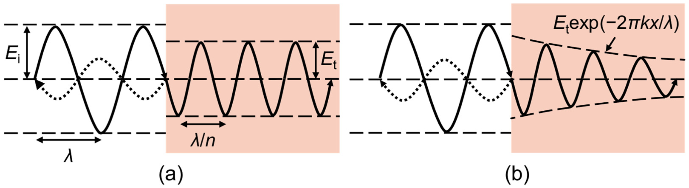
2.1.1. Reflection from a Bulk Surface

When light is incident on an object, it undergoes multiple absorptions, reflections, and transmissions at the surface, and the color of that object is determined by the spectrum of light reflected from its surface. Fresnel equations describe the reflected and transmitted amplitudes of light with respect to that of the incident wave, which can be derived from the boundary conditions of electric and magnetic fields at an interface.

We define the plane of incidence that contains the surface normal vector and the propagation vector of incident light and determine p- or s-polarization from the direction of E oscillation with respect to the plane of incidence (Figure 1). The p-polarization indicates that E oscillates parallel to the plane of incidence (Figure 1a). Here, we first derive the Fresnel equations for the case of polarization parallel to the plane of incidence (i.e., p-polarization). Since the parallel component of E and the normal component of B with respect to the interface need to be continuous, we arrive at the following equations:

$$E_{\mathrm{i}}\cos {\mathit{\theta }}_{\mathrm{i}}-E_{\mathrm{r}}\cos {\mathit{\theta }}_{\mathrm{r}}=E_{\mathrm{t}}\cos {\mathit{\theta }}_{\mathrm{t}}$$

(1)

$${\mathit{B}}_{\mathrm{i}}+{ \mathit{B}}_{\mathrm{r}}={ \mathit{B}}_{\mathrm{t}}$$

(2)

where the subscripts i, r, and t represent the incident, reflected, and transmitted waves, respectively. Since $\mathit{B}=E·n/c$ (n: refractive index,$n \equiv c/v$) where $v$ is the speed of an electromagnetic wave in matter [23], Equation (2) indicates that

$$n_{\mathrm{i}}\left(E_{\mathrm{i} }+E_{\mathrm{r}}\right)=n_{\mathrm{t}}{E}_{\mathrm{t}}$$

(3)

where $n_{\mathrm{i}}$ and $n_{\mathrm{t}}$ are the refractive indices of the media before and after transmission. Given the laws of reflection (${\mathit{\theta }}_{\mathrm{r}}={\mathit{\theta }}_{\mathrm{i}}$) and refraction (i.e., Snell’s law; $n_{\mathrm{i}}\sin {\mathit{\theta }}_{\mathrm{i}}=n_{\mathrm{t}}\sin {\mathit{\theta }}_{\mathrm{t}}$) and by solving Equations (1) and (2), we obtain the reflection and transmission coefficients for p-polarized light:

$$r_{\mathrm{p}} \equiv {\displaystyle \frac{E_{\mathrm{r}}}{E_{\mathrm{i}}}}={\displaystyle \frac{n_{\mathrm{t}}\cos {\mathit{\theta }}_{\mathrm{i}}-n_{\mathrm{i}}\cos {\mathit{\theta }}_{\mathrm{t}}}{n_{\mathrm{t}}\cos {\mathit{\theta }}_{\mathrm{i}}+{ n}_{\mathrm{i}}\cos {\mathit{\theta }}_{\mathrm{t}}}}$$

(4)

$$t_{\mathrm{p}} \equiv {\displaystyle \frac{E_{\mathrm{t}}}{E_{\mathrm{i}}}}={\displaystyle \frac{2n_{\mathrm{i}}\cos {\mathit{\theta }}_{\mathrm{i}}}{n_{\mathrm{t}}\cos {\mathit{\theta }}_{\mathrm{i}}+n_{\mathrm{i}}\cos {\mathit{\theta }}_{\mathrm{t}}}}.$$

(5)

For s-polarization (Figure 1b), the boundary conditions for E and B become

$$E_{\mathrm{i}}+E_{\mathrm{r}}=E_{\mathrm{t}}$$

(6)

$${-\mathit{B}}_{\mathrm{i}}\cos {\mathit{\theta }}_{\mathrm{i}}-{\mathit{B}}_{\mathrm{r}}\cos {\mathit{\theta }}_{\mathrm{r}}={-\mathit{B}}_{\mathrm{t}}\cos {\mathit{\theta }}_{\mathrm{t}}.$$

(7)

The reflection and transmission coefficients for s-polarized light can be obtained by the same procedure.

$$r_{\mathrm{s}} \equiv {\displaystyle \frac{E_{\mathrm{r}}}{E_{\mathrm{i}}}}={\displaystyle \frac{n_{\mathrm{i}}\cos {\mathit{\theta }}_{\mathrm{i}}-n_{\mathrm{t}}\cos {\mathit{\theta }}_{\mathrm{t}}}{n_{\mathrm{i}}\cos {\mathit{\theta }}_{\mathrm{i}}+n_{\mathrm{t}}\cos {\mathit{\theta }}_{\mathrm{t}}}}$$

(8)

$$t_{\mathrm{s}} \equiv {\displaystyle \frac{E_{\mathrm{t}}}{E_{\mathrm{i}}}}={\displaystyle \frac{2n_{\mathrm{i}}\cos {\mathit{\theta }}_{\mathrm{i}}}{n_{\mathrm{i}}\cos {\mathit{\theta }}_{\mathrm{i}}+n_{\mathrm{t}}\cos {\mathit{\theta }}_{\mathrm{t}}}}.$$

(9)

The reflectance (R) and transmittance (T) are defined by the ratio of the reflected and transmitted intensity (average power per unit area) to the incident intensity ($I=1/2ϵv{E}^2$); thus,

$$R \equiv {\displaystyle \frac{I_{\mathrm{r}}}{I_{\mathrm{i}}}}={\left|{\displaystyle \frac{E_{\mathrm{r}}}{E_{\mathrm{i}}}}\right|}^2={ \left|r\right|}^2$$

(10)

$$T \equiv {\displaystyle \frac{I_t\cos {\mathit{\theta }}_{\mathrm{t}}}{I_{\mathrm{i}}\cos {\mathit{\theta }}_{\mathrm{i}}}}=\left({\displaystyle \frac{n_{\mathrm{t}}\cos {\mathit{\theta }}_{\mathrm{t}}}{n_{\mathrm{i}}\cos {\mathit{\theta }}_{\mathrm{i}}}}\right){\left|{\displaystyle \frac{E_{\mathrm{t}}}{E_{\mathrm{i}}}}\right|}^2=\left({\displaystyle \frac{n_{\mathrm{t}}\cos {\mathit{\theta }}_{\mathrm{t}}}{n_{\mathrm{i}}\cos {\mathit{\theta }}_{\mathrm{i}}}}\right){\left|t\right|}^2.$$

(11)

The reflectance depends on the polarization of the light, and we consider natural, or unpolarized, light in this article. The reflectance of unpolarized light (R_n) can be given by the averaged reflectance of all incident waves with different polarization angles:

$$R_{\mathrm{n} }={\displaystyle \frac{1}{2\pi }}{\int }_{-\pi }^{\pi }{R}_{\mathsf{\psi }}d\psi ={\displaystyle \frac{\left(R_{\mathrm{p}}+R_{\mathrm{s}}\right)}{2}}$$

(12)

where $\psi$ is the polarization angle [24].

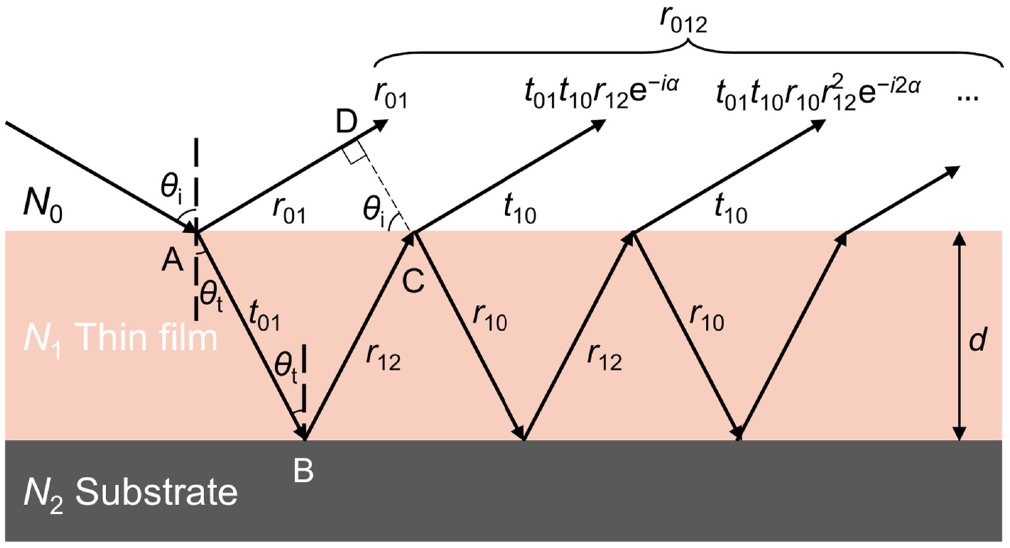
2.1.2. Reflection from a (Multilayered) Thin Film

For a thin film or multilayered structure, we need to consider the absorption and optical interference of multiple reflections, transmissions, and absorptions occurring at interfaces underneath the surface.

This absorption can be formulated by incorporating a complex refractive index into the wave function (Figure 2). The wave function of a plane wave traveling in the x direction can be written in complex notation as follows:

$$\stackrel{\mathrm{~}}{\mathbf{E}}={\stackrel{\mathrm{~}}{\mathbf{E}}}_0\exp [i(\omega t-\tilde{K}x\left)\right]$$

(13)

where ${\stackrel{\mathrm{~}}{\mathbf{E}}}_0$, $\omega$, t, $\tilde{K}$, and x are the complex wave amplitude’s, angular frequency, time, complex wavenumber, and position, respectively. The complex wavenumber can be written as

$$\stackrel{\mathrm{~}}{K} \equiv {\displaystyle \frac{2\pi \stackrel{\mathrm{~}}{N}}{\lambda }}$$

(14)

where $\stackrel{\mathrm{~}}{N}$ is the complex refractive index. $\stackrel{\mathrm{~}}{N}$ is defined as

$$\stackrel{\mathrm{~}}{N} \equiv n-\mathit{ik}$$

(15)

where n and k are the refractive index and extinction coefficient, respectively. By substituting Equations (14) and (15) into Equation (13), we obtain an expression for the electromagnetic wave that takes attenuation (i.e., exponential decay) due to the absorption into account:

$$\stackrel{\mathrm{~}}{\mathbf{E}}={\stackrel{\mathrm{~}}{\mathbf{E}}}_0\exp \left(-{\displaystyle \frac{2\pi \mathit{kx}}{\lambda }}\right)·\exp \left[i\left(\omega t-{\displaystyle \frac{2\pi n}{\lambda }}x\right)\right].$$

(16)

In addition to absorption, we need to consider optical interference. Figure 3 shows the presence of reflected light from the interfaces between (1) air and the thin film (upper) and (2) the thin film and its substrate (lower). The reflected light waves will interfere either constructively or destructively, depending on the phase difference between the two waves. The path length difference between the two waves is $\stackrel{-}{\mathrm{AB}}+\stackrel{-}{\mathrm{BC}}-\stackrel{-}{\mathrm{AD}}$. The paths $\stackrel{-}{\mathrm{AB}}$ and $\stackrel{-}{\mathrm{BC}}$ traverse a medium with a refractive index of $N_1$, while path $\stackrel{-}{\mathrm{AD}}$ traverses a medium with a refractive index of $N_0$. Therefore, the phase difference ($\alpha$) is obtained by applying the different wavenumbers ($K=2\pi N/\lambda$) as follows:

$$\alpha ={\displaystyle \frac{2\pi N_1}{\lambda }}\left(\stackrel{-}{\mathrm{AB}}+\stackrel{-}{\mathrm{BC}}\right)-{\displaystyle \frac{2\pi N_0}{\lambda }}\stackrel{-}{\mathrm{AD}}.$$

(17)

Considering the incident and transmitted angles, we obtain $\stackrel{-}{\mathrm{AD}}=\stackrel{-}{\mathrm{AC}}\sin {\mathit{\theta }}_{\mathrm{i}}$ and $\stackrel{-}{\mathrm{AC}}=2d\tan {\mathit{\theta }}_{\mathrm{t}}$, which lead to

$$\stackrel{-}{\mathrm{AD}}=2d\tan {\mathit{\theta }}_{\mathrm{t}}·\sin {\mathit{\theta }}_{\mathrm{i}}.$$

(18)

By incorporating Snell’s law ($\sin {\mathit{\theta }}_{\mathrm{i}}=\sin {\mathit{\theta }}_{\mathrm{t}}{N}_1/N_0$),

$$\stackrel{-}{\mathrm{AD}}=2d{\displaystyle \frac{{\sin }^2{\mathit{\theta }}_{\mathrm{t}}}{\cos {\mathit{\theta }}_{\mathrm{t}}}}·{\displaystyle \frac{N_1}{N_0}}.$$

(19)

Using Equation (19) and $\stackrel{-}{\mathrm{AB}}=\stackrel{-}{\mathrm{BC}}=d/\cos {\mathit{\theta }}_{\mathrm{t}}$, we arrive at

$$\alpha ={\displaystyle \frac{4\pi d{N}_1}{\lambda }} · \cos {\mathit{\theta }}_{\mathrm{t}}.$$

(20)

The plane wave, when considering the phase difference, becomes

$$\exp \left[i\left\{\omega t-\left(\mathit{Kr}+\alpha \right)\right\}\right]=\exp \left[i\left(\omega t-\mathit{Kr}\right)\right] · \exp \left(-i\alpha \right).$$

(21)

Equation (21) indicates that the phase difference can be imposed by multiplying $\exp \left(-i\alpha \right)$. To account for the optical interference, we need to find the superposition of the light waves which are reflected from both upper and lower boundaries. The primary wave (i.e., that directly reflected from the film surface) becomes $E_1={r_{01}E}_{\mathrm{i}}$, which is the reflection coefficient determined by the Fresnel equations for the boundary between the air and the thin film. The secondary wave, which is transmitted at the boundary between the air and the thin film, is then reflected from the substrate and transmitted at the boundary between the thin film and air and can be written by imposing the coefficients corresponding to each stage as follows:

$$E_2=t_{01}{t}_{10}{r}_{12}\exp \left(-i\alpha \right)E_{\mathrm{i}}.$$

(22)

As each additional order is considered, the wave undergoes two reflections (r₁₀ and r₁₂) and acquires a phase difference. Each subsequent term is multiplied by a factor of ${r_{10}r}_{12}\exp \left(-i\alpha \right)$. The total reflected wave (E₀₁₂) can be expressed as the sum of the primary wave (E₁), the secondary wave (E₂), the third wave (E₃), and so on:

$$\begin{array}{c}{E}_{012}=(r_{01 }+t_{01}{t}_{10}{r}_{12}\exp \left(-i\alpha \right)+{t_{01}{t}_{10}{r}_{10}{r}_{12}^2\exp \left(-i2\alpha \right)+\dots )E}_{\mathrm{i}}\\ =[r_{01 }+t_{01}{t}_{10}{\displaystyle \sum _{\mathrm{m}=1}^{\infty }}{r}_{10}^{m-1}{r}_{12}^{\mathrm{m}}\exp \left(-\mathrm{m}i\alpha \right)]E_{\mathrm{i}}=r_{012}{E}_{\mathrm{i}}.\end{array}$$

(23)

$r_{012}$ thus represents the reflection coefficient obtained when considering the optical interference. Using the formula for the sum of an infinite geometric series, we can simply write Equation (23) as

$$r_{012}=r_{01}+{\displaystyle \frac{t_{01}{t}_{10}{r}_{12}\exp \left(-i\alpha \right)}{1-r_{10}{r}_{12}\exp \left(-i\alpha \right)}}.$$

(24)

Using $r_{10}=-r_{01}$ and $t_{01}{t}_{10}=1-r_{01}^2$, obtained by Equations (4), (5), (8), and (9), $r_{012}$ can be reduced further [25]:

$$r_{012}={\displaystyle \frac{r_{01}+r_{12}\exp \left(-\mathrm{i}\alpha \right)}{1+r_{01}{r}_{12}\exp \left(-\mathrm{i}\alpha \right)}}.$$

(25)

Using Equation (25), the reflection coefficient for the air/thin film/substrate structure (Figure 3) can be obtained. Based on Equation (25), additional layers can be incorporated. When an additional layer is introduced (e.g., the buffer layer in an air/thin film/buffer layer/substrate structure), the reflection coefficient $r_{0123}$ is derived. To determine $r_{0123}$, Equation (25) is first applied to compute $r_{123}$:

$$r_{123}={\displaystyle \frac{r_{12}+r_{23}\exp \left(-i\alpha \right)}{1+{ r}_{12}{r}_{23}\exp \left(-i\alpha \right)}}.$$

(26)

By substituting $r_{123}$, obtained from Equation (26), into the $r_{12}$ term in Equation (25), the expression for $r_{0123}$ is obtained as follows:

$$r_{0123}={\displaystyle \frac{r_{01}+r_{123}\exp \left(-i\alpha \right)}{1+{ r}_{01}{r}_{123}\exp \left(-i\alpha \right)}}.$$

(27)

This recursive approach, based on Equation (25), allows us to determine the reflection coefficient of a multilayer structure with an arbitrary number of layers. Using Equations (10) and (27), we can obtain the reflectance of multilayered structures for a specific single wavelength. To simulate the color, we need to obtain the reflectance spectrum in the visible range, which thus requires us to use different refractive indices and extinction coefficients depending on the wavelength (i.e., dispersion) for the visible range.

2.1.3. Color Simulation

To convert a reflectance spectrum to a color (i.e., sRGB value), the spectrum is first mapped to the CIE 1931 XYZ color space using formulas based on color matching functions [26]:

$$N=\int \stackrel{-}{y}\left(\lambda \right)I\left(\lambda \right)d\lambda$$

(28)

$$X={\displaystyle \frac{1}{N}}\int \stackrel{-}{x}\left(\lambda \right)S\left(\lambda \right)I\left(\lambda \right)d\lambda$$

(29)

$$Y={\displaystyle \frac{1}{N}}\int \stackrel{-}{y}\left(\lambda \right)S\left(\lambda \right)I\left(\lambda \right)d\lambda$$

(30)

$$Z={\displaystyle \frac{1}{N}}\int \stackrel{-}{z}\left(\lambda \right)S\left(\lambda \right)I\left(\lambda \right)d\lambda$$

(31)

where $\lambda$ is the wavelength and $\overline{x}$, $\overline{y}$, and $\overline{z}$ are the color-matching functions, which are numerical descriptions of the chromatic and tristimulus response of cone cells [27]. The parameters $S\left(\lambda \right)$ and $I\left(\lambda \right)$ are the spectral reflectance and standard illuminant, respectively. In this study, we employed a CIE 1931 2° standard observer and D65 white reference as the color matching functions and the reference illuminant, respectively [28,29]. The CIE 1931 2° standard observer quantifies human color perception. Due to the distribution of cones in the human eye, the tristimulus values of colors vary depending on the observer’s field of view. The standard observer model was defined based on stimuli subtending a 2° visual angle, corresponding to the foveal region of the retina. The D65 white reference is the standard daylight illuminant, positioned using CIE values. The values X, Y, and Z can be converted to either CIE xy values or sRGB values. For CIE xy values,

$$x={\displaystyle \frac{X}{X+Y+Z}}$$

(32)

$$y={\displaystyle \frac{Y}{X+Y+Z}}$$

(33)

where x and y are the coordinates of the CIE 1931 color space chromaticity diagram, which is widely used to specify colors in practice. CIE XYZ coordinates are linearly transformed to sRGB coordinates using the following conversion matrix [30]:

$$\left[\begin{array}{c}r\\ g\\ b\end{array}\right]=\left[\begin{array}{ccc}3.24045& -1.53714& -0.49853\\ -0.96927& 1.87601& 0.04156\\ 0.05564& -0.20403& 1.05723\end{array}\right]\left[\begin{array}{c}X\\ Y\\ Z\end{array}\right]$$

(34)

where r, g, and b are linear RGB. The sRGB color space defines its values in a nonlinear form that corresponds to human visual perception. However, the conversion from XYZ to RGB derived above produces linear RGB values. To obtain sRGB values, a gamma-compressed transformation is used [30]:

$$V=\left\{\begin{array}{cc}12.92v& v \le 0.0031308\\ 1.055v^{1/2.4}-0.055& \mathrm{otherwise}\end{array}\right.$$

(35)

where $v\in \left\{r, g, b\right\}$ and $V\in \left\{R, G, \mathit{B}\right\}$. Since the values obtained using Equation (35) are in the nominal range (0–1), we multiply each component by 255 to represent conventional sRGB values in the range of 0–255.

2.2. Python Coding

Based on the aforementioned theoretical background, we developed a Python 3.9.13 code to simulate the colors of multilayered thin films. We imported libraries—NumPy, pandas, SciPy, and matplotlib—for numerical computations, data manipulation, interpolation, and visualization, respectively. A wavelength array in the visible range with a fixed step size was generated using the arange function in the NumPy library (line 2 in Listing 1). To use the dispersion relation of each layer, we needed to import the refractive indices (n) and extinction coefficients (k) of the wavelengths in the array (lines 4–10 in Listing 1). Using this code, we aimed to simulate the color of SnO₂ layers on a Si substrate, which has a native oxide layer; thus we used the n and k values of SnO₂, SiO₂, and Si from the literature [31,32,33,34]. We imported a standard illuminant (D65) and applied it to the obtained reflectance spectra to simulate the spectra from the sample, and the color-matching functions (CMFs) were imported and applied to extract RGB values from the simulated spectra (lines 35–42 in Listing 1). Here, missing n, k, and CMFs values, which are required but absent in the literature, can be estimated by interpolation using the interp1d function in the SciPy library. Since both the extinction coefficients and dispersion of air in the visible range are negligible, we set the refractive index of air as the constant, 1.0003, and defined the imaginary unit as j (lines 12–15 in Listing 1).

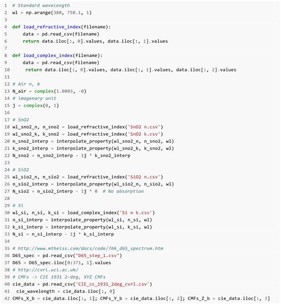
Listing 1. Python code for data preprocessing.

The reflection coefficients of the p- and s-polarized waves and the reflectance are calculated in lines 1–10 and lines 11–45 of Listing 2, respectively. Here, N_j and N_k indicate the complex refractive indices of media j and k, respectively. ang_j and ang_k are the angles of incidence and transmission, respectively. In line 11 of Listing 2, wl, N_0, N_1, N_2, and N_3 are the wavelength and the complex refractive indices of the atmosphere (i.e., air), top, middle, and bottom layers (here the bottom layer corresponds to the substrate), respectively. d_1, and d_2 are the thicknesses of the top and middle layers, respectively. The mathematical expression corresponding to each line of code is given above it using the equation numbers described in Section 2.1 (Theoretical Background).

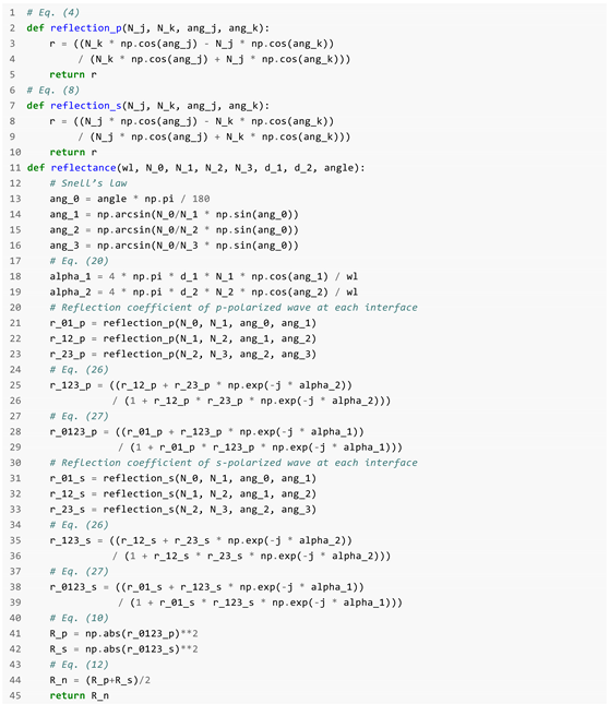
Listing 2. Python code used to calculate the reflection coefficients and the reflectance.

By modifying the values of d_1, d_2, and the angle in line 11 of Listing 2, we can obtain reflectance spectra for various thicknesses and incident ray angles. To convert the reflectance spectra into RGB values, we apply Listing 3; in line 1, R_n is the calculated reflectance spectrum, while D65, CMFs_X, CMFs_Y, and CMFs_Z are the standard illuminant and the color matching functions for X, Y, and Z, respectively, which were imported and defined earlier (in line 38–42 of Listing 1).

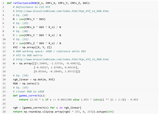
Listing 3. Python code used to convert the reflectance spectrum to RGB values.

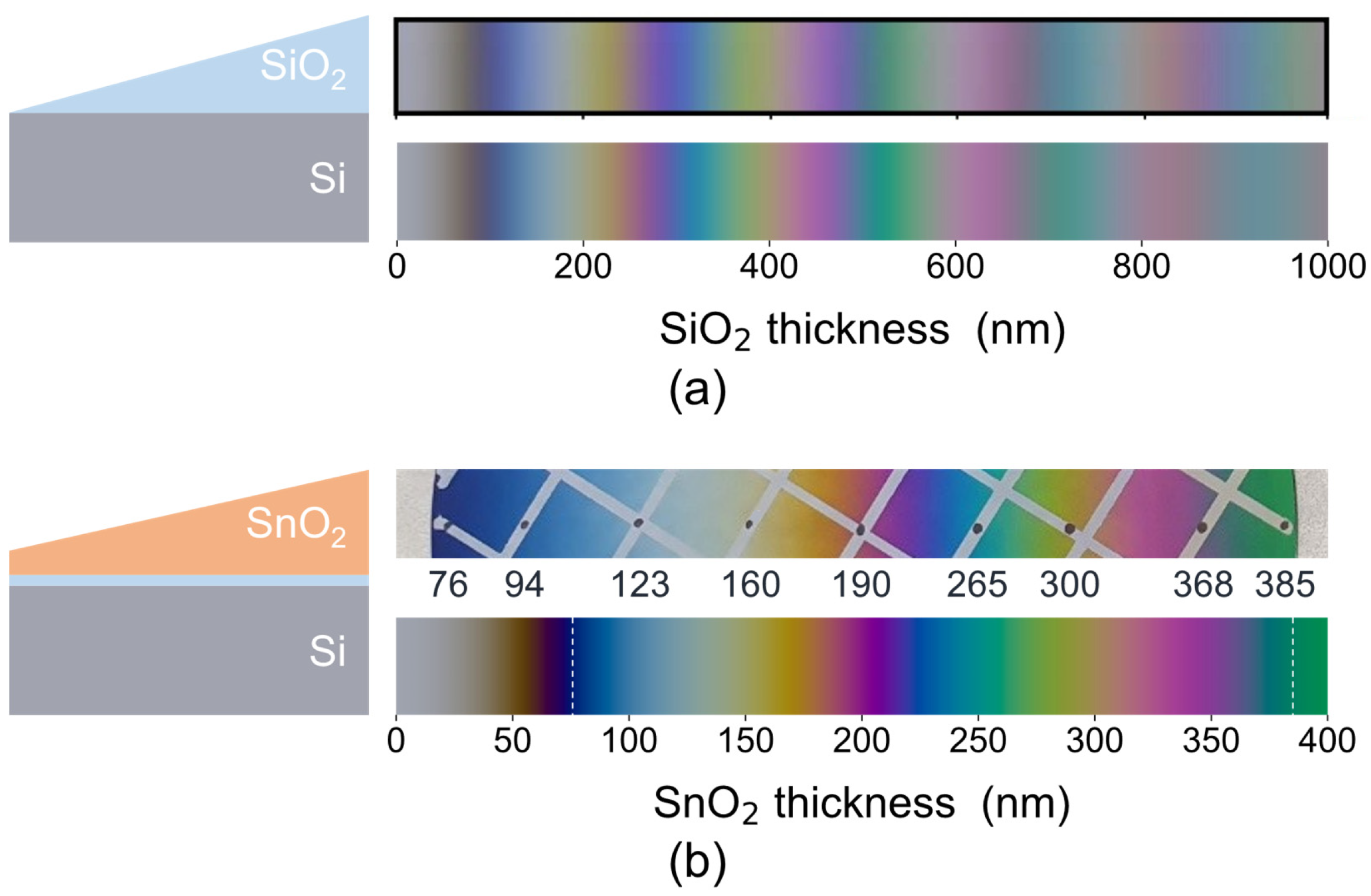
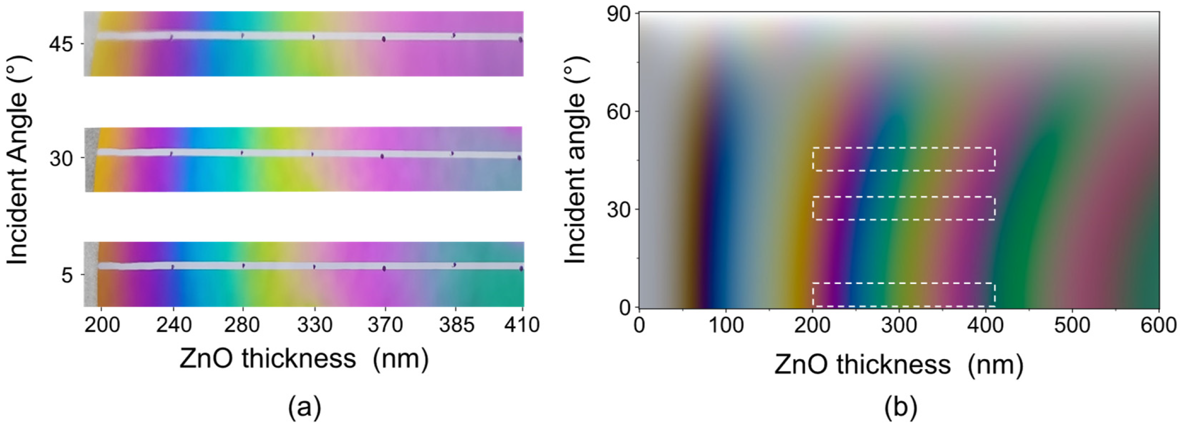
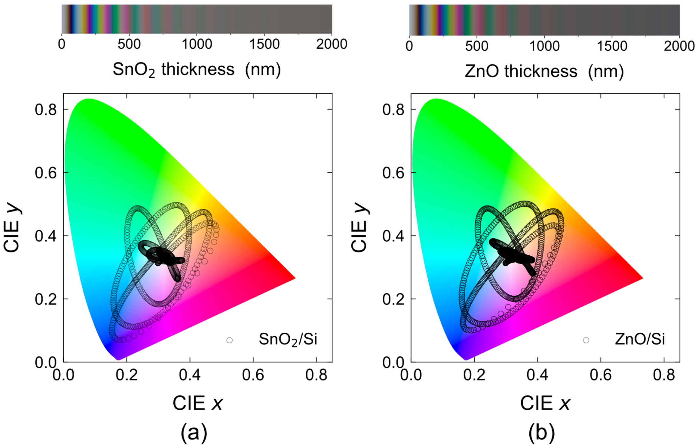
3. Results and Discussion

To validate the Python code used for simulating the color of multilayered structures, we simulated the colors of three different oxide thin films (SiO₂, SnO₂, and ZnO) deposited on a Si substrate as a function of the films’ thickness and compared them with the literature and our own experiment. We first checked the color of the SiO₂ thin film on a Si substrate using a function of the film thickness. It can be clearly seen that the obtained color chart is very consistent with the reported simulation result (Figure 4a) [35]. For the comparative analysis with our experiment, we fabricated a SnO₂ film with a thickness gradient on a Si wafer using a sputtering method and measured its thicknesses by performing line profile measurements across a masked area using noncontact (tapping mode) atomic force microscopy (AFM; Icon-PT-PLUS, Bruker, Germany). For each point, three independent line profile measurements were taken to obtain average thickness and estimate the standard deviation. The step size of the line profile measurements was 1.5 μm, and the standard deviation of the thickness values was generally around 0.3 nm. The base pressure was ≈3 × 10⁻⁸ Torr, and the working pressure of 10 mTorr was adjusted using Ar (99.9999%). The films were grown at room temperature. We assumed the presence of a 2 nm thick native oxide layer (SiO₂) between the film and substrate [36,37]. The two white dashed lines in Figure 4b indicate the experimentally measured thickness range (i.e., 76–385 nm). Although the thickness gradient of the experimental samples is nonlinear with respect to the position of each measured point, the colors and the thicknesses measured at the nine points are in good agreement with the theoretically predicted colors and thicknesses.

Figure 5a shows the experimental colors of a ZnO thin film with a thickness gradient on a Si substrate, taken at different incident angles (5, 30, and 45°). Similarly to the SnO₂ thin film, we fabricated the ZnO film using the sputtering method and measured its thicknesses using AFM. As the incident angle increases, the overall color gradient shifts toward the thicker region, and as the thickness increases, the gradient becomes more pronounced. For instance, the color of the film changes from blue to magenta at 240 nm and from cyan to pink at 410 nm as the angle varies. To visualize the change in the color gradient, we simulated the colors of the ZnO thin film on a Si substrate, with a 2 nm thick SiO₂ layer in between the two, as a function of the thickness and angle (Figure 5b). In this simulation, we used the n and k values of ZnO from the literature [38]. The simulation results obtained using the Python code describe the experimental color variations as depending on both thicknesses and incident angles. The three white boxes in Figure 5b represent the color ranges expected for the given thicknesses and angle variations in the experimental sample. The theoretical results clearly demonstrate the color transition seen due to the change in angle: from cyan to pink in the thicker regions and with an expansion of the yellow region in the thinner regions.

So far, we have obtained CIE XYZ values from simulated reflectance spectra and have converted them into sRGB for more intuitive color representations. Additionally, using Equations (32) and (33), we can transform CIE XYZ into CIE xy, allowing us to map the colors onto the CIE 1931 color space. This two-dimensional color space facilitates the identifying of color differences and supports a device- and observer-independent color representations suitable for various display and printing applications. Figure 6 shows the simulated colors of the SnO₂ and ZnO thin films represented in both the sRGB and CIE xy color spaces. In the sRGB representation, the fact that the color variations are a function of thickness is easily observable. In contrast, the CIE xy representation provides insight into the color gamut achievable from a given material. For example, although the colors of SnO₂ and ZnO appear similar in the RGB color space, the CIE color space reveals that SnO₂ can be used to produce a slightly more vivid blue.

The results above demonstrate the ability of the Python code to create accurate reflectance spectra and corresponding color simulations. This code could be developed further to estimate the thickness of a film based on known n and k values, and vice versa. Moreover, recent advances in materials research have increasingly made use of AI-driven approaches, such as optics-based inverse design [39,40,41,42,43,44,45] and active learning [46]. In this context, this code, implemented in Python, which has been primarily used in AI research, serves as an accessible and easily modifiable, yet powerful, tool.

4. Conclusions

We demonstrated that our Python script can simulate the color of multilayered structures, with a detailed theoretical background and annotations provided for readers as well as users. The developed code was validated by applying it to well-known oxide materials (SnO₂ and ZnO). We believe that anyone can adjust its structural and material parameters for their own system and research by following the instructions presented here. It is also worthwhile noting that the code generates a substantial quantity of data very rapidly—for example, simulating the 54,000 colors displayed in Figure 5b took merely 52 s (using CPU: Intel i7-1255U; GPU: Intel Iris Xe Graphics). This code can be further used and developed for various purposes—especially for machine learning, which requires a large amount of spectral and color data for model training.

References

1. Li, K.; Li, T.; Zhang, T.; Li, H.; Li, A.; Li, Z.; Lai, X.; Hou, X.; Wang, Y.; Shi, L.; et al. Facile full-color printing with a single transparent ink. Sci. Adv. 2021, 7, eabh1992. [Google Scholar] [CrossRef] [PubMed]
2. Li, R.; Li, K.; Deng, X.; Jiang, C.; Li, A.; Xue, L.; Yuan, R.; Liu, Q.; Zhang, Z.; Li, H.; et al. Dynamic High-Capacity Structural-Color Encryption via Inkjet Printing and Image Recognition. Adv. Funct. Mater. 2024, 34, 2404706. [Google Scholar] [CrossRef]
3. Yang, Y.; Kim, J.B.; Nam, S.K.; Zhang, M.; Xu, J.; Zhu, J.; Kim, S.-H. Nanostructure-free crescent-shaped microparticles as full-color reflective pigments. Nat. Commun. 2023, 14, 793. [Google Scholar] [CrossRef] [PubMed]
4. Kim, S.J.; Kim, S.; Lee, J.; Jo, Y.; Seo, Y.-S.; Lee, M.; Lee, Y.; Cho, C.R.; Kim, J.-p.; Cheon, M.; et al. Color of Copper/Copper Oxide. Adv. Mater. 2021, 33, 2007345. [Google Scholar] [CrossRef]
5. Huang, Y.-S.; Lee, C.-Y.; Rath, M.; Ferrari, V.; Yu, H.; Woehl, T.J.; Ni, J.H.; Takeuchi, I.; Ríos, C. Tunable structural transmissive color in fano-resonant optical coatings employing phase-change materials. Mater. Today Adv. 2023, 18, 100364. [Google Scholar] [CrossRef]
6. Lu, Y.; Shi, X.; Huang, Z.; Li, T.; Zhang, M.; Czajkowski, J.; Fabritius, T.; Huttula, M.; Cao, W. Nanosecond laser coloration on stainless steel surface. Sci. Rep. 2017, 7, 7092. [Google Scholar] [CrossRef]
7. Badloe, T.; Kim, J.; Kim, I.; Kim, W.-S.; Kim, W.S.; Kim, Y.-K.; Rho, J. Liquid crystal-powered Mie resonators for electrically tunable photorealistic color gradients and dark blacks. Light Sci. Appl. 2022, 11, 118. [Google Scholar] [CrossRef]
8. Lee, D.-J. Thin Film Interference. Available online: https://javalab.org/en/thin_film_interference_en/ (accessed on 24 March 2025).
9. Oskooi, A.F.; Roundy, D.; Ibanescu, M.; Bermel, P.; Joannopoulos, J.D.; Johnson, S.G. Meep: A flexible free-software package for electromagnetic simulations by the FDTD method. Comput. Phys. Commun. 2010, 181, 687–702. [Google Scholar] [CrossRef]
10. JA Woollam. Guide to Using WVASE32®; JA Woollam: Lincoln, NE, USA, 2002; p. 529. [Google Scholar]
11. Kruschke, J. Doing Bayesian Data Analysis: A Tutorial with R, JAGS, and Stan; Elsevier: Amsterdam, The Netherlands, 2014. [Google Scholar]
12. Lohumi, S.; Lee, H.; Kim, M.S.; Qin, J.; Cho, B.-K. Raman Imaging for the Detection of Adulterants in Paprika Powder: A Comparison of Data Analysis Methods. Appl. Sci. 2018, 8, 485. [Google Scholar] [CrossRef]
13. Kurth, M.; Graat, P.C.J.; Mittemeijer, E.J. Determination of the intrinsic bulk and surface plasmon intensity of XPS spectra of magnesium. Appl. Surf. Sci. 2003, 220, 60–78. [Google Scholar] [CrossRef]
14. Montoya-Escobar, N.; Ospina-Acero, D.; Velásquez-Cock, J.A.; Gómez-Hoyos, C.; Serpa Guerra, A.; Gañan Rojo, P.F.; Vélez Acosta, L.M.; Escobar, J.P.; Correa-Hincapié, N.; Triana-Chávez, O.; et al. Use of Fourier Series in X-ray Diffraction (XRD) Analysis and Fourier-Transform Infrared Spectroscopy (FTIR) for Estimation of Crystallinity in Cellulose from Different Sources. Polymers 2022, 14, 5199. [Google Scholar] [CrossRef] [PubMed]
15. Agostinelli, S.; Allison, J.; Amako, K.; Apostolakis, J.; Araujo, H.; Arce, P.; Asai, M.; Axen, D.; Banerjee, S.; Barrand, G.; et al. Geant4—A simulation toolkit. Nucl. Instrum. Methods Phys. Res. Sect. A Accel. Spectrom. Detect. Assoc. Equip. 2003, 506, 250–303. [Google Scholar] [CrossRef]
16. Blocken, B.; Stathopoulos, T.; Carmeliet, J. CFD simulation of the atmospheric boundary layer: Wall function problems. Atmos. Environ. 2007, 41, 238–252. [Google Scholar] [CrossRef]
17. Kok, C.L.; Ho, C.K.; Taufik, A.S.; Koh, Y.Y.; Teo, T.H. Development of a Sustainable Universal Python Code for Accurate 2D Heat Transfer Conduction Simulations in Educational Environment. Appl. Sci. 2024, 14, 7159. [Google Scholar] [CrossRef]
18. Luce, A.; Mahdavi, A.; Marquardt, F.; Wankerl, H. TMM-Fast, a transfer matrix computation package for multilayer thin-film optimization: Tutorial. J. Opt. Soc. Am. A 2022, 39, 1007–1013. [Google Scholar] [CrossRef]
19. Thelen, F.; Zehl, R.; Bürgel, J.L.; Depla, D.; Ludwig, A. A python-based approach to sputter deposition simulations in combinatorial materials science. Surf. Coat. Technol. 2025, 503, 131998. [Google Scholar] [CrossRef]
20. Ketkar, N.; Santana, E. Deep Learning with Python; Apress: Berkeley, CA, USA, 2017; Volume 1. [Google Scholar]
21. Pedregosa, F.; Varoquaux, G.; Gramfort, A.; Michel, V.; Thirion, B.; Grisel, O.; Blondel, M.; Prettenhofer, P.; Weiss, R.; Dubourg, V. Scikit-learn: Machine learning in Python. J. Mach. Learn. Res. 2011, 12, 2825–2830. [Google Scholar]
22. Raschka, S.; Mirjalili, V. Python Machine Learning: Machine Learning and Deep Learning with Python, Scikit-Learn, and TensorFlow 2; Packt Publishing Ltd: Birmingham, UK, 2019. [Google Scholar]
23. Griffiths, D.J. Introduction to Electrodynamics; Cambridge University Press: Cambridge, UK, 2023. [Google Scholar]
24. Zhao, B.; Sakurai, A.; Zhang, Z.M. Polarization Dependence of the Reflectance and Transmittance of Anisotropic Metamaterials. J. Thermophys. Heat Transf. 2015, 30, 240–246. [Google Scholar] [CrossRef]
25. Fujiwara, H. Spectroscopic Ellipsometry: Principles and Applications; John Wiley & Sons: Hoboken, NJ, USA, 2007. [Google Scholar]
26. Lindbloom, B. Rgb/xyz Matrices. Available online: http://www.brucelindbloom.com/index.html (accessed on 24 March 2025).
27. Stockman, A.; Sharpe, L.T. Cone Spectral Sensitivities and Color Matching; Cambridge U. Press: Cambridge, UK, 1999; pp. 53–88. [Google Scholar]
28. CIE2019. Colour-Matching Functions of CIE 1931 Standard Colorimetric Observer. Available online: https://doi.org/10.25039/CIE.DS.xvudnb9b (accessed on 24 March 2025).
29. CIE2019. CIE Standard Illuminant D65. Available online: https://doi.org/10.25039/CIE.DS.hjfjmt59 (accessed on 24 March 2025).
30. IEC 61966-2-1:1999; Multimetdia Systems and Equipment—Colour Measurement and Management—Part 2-1: Colour Management—Default RGB Colour Space—SRGB. CIE: Vienna, Austria, 1999.
31. Arosa, Y.; de la Fuente, R. Refractive index spectroscopy and material dispersion in fused silica glass. Opt. Lett. 2020, 45, 4268–4271. [Google Scholar] [CrossRef]
32. Polyanskiy, M.N. Refractiveindex.info database of optical constants. Sci. Data 2024, 11, 94. [Google Scholar] [CrossRef]
33. Prasanth, A.; Meher, S.R.; Alex, Z.C. Experimental analysis of SnO2 coated LMR based fiber optic sensor for ethanol detection. Opt. Fiber Technol. 2021, 65, 102618. [Google Scholar] [CrossRef]
34. Schinke, C.; Christian Peest, P.; Schmidt, J.; Brendel, R.; Bothe, K.; Vogt, M.R.; Kröger, I.; Winter, S.; Schirmacher, A.; Lim, S.; et al. Uncertainty analysis for the coefficient of band-to-band absorption of crystalline silicon. AIP Adv. 2015, 5, 067168. [Google Scholar] [CrossRef]
35. Henrie, J.; Kellis, S.; Schultz, S.M.; Hawkins, A. Electronic color charts for dielectric films on silicon. Opt. Express 2004, 12, 1464–1469. [Google Scholar] [CrossRef]
36. Ceresa, E.M.; Garbassi, F. AES/XPS Thickness measurement of the native oxide on single crystal Si wafers. Mater. Chem. Phys. 1983, 9, 371–385. [Google Scholar] [CrossRef]
37. Morita, M.; Ohmi, T.; Hasegawa, E.; Kawakami, M.; Ohwada, M. Growth of native oxide on a silicon surface. J. Appl. Phys. 1990, 68, 1272–1281. [Google Scholar] [CrossRef]
38. Aguilar, O.; de Castro, S.; Godoy, M.P.F.; Rebello Sousa Dias, M. Optoelectronic characterization of Zn1−xCdxO thin films as an alternative to photonic crystals in organic solar cells. Opt. Mater. Express 2019, 9, 3638–3648. [Google Scholar] [CrossRef]
39. Head, S.; Keshavarz Hedayati, M. Inverse Design of Distributed Bragg Reflectors Using Deep Learning. Appl. Sci. 2022, 12, 4877. [Google Scholar] [CrossRef]
40. Huang, Z.; Liu, X.; Zang, J. The inverse design of structural color using machine learning. Nanoscale 2019, 11, 21748–21758. [Google Scholar] [CrossRef]
41. Liu, Z.; Zhu, D.; Raju, L.; Cai, W. Tackling Photonic Inverse Design with Machine Learning. Adv. Sci. 2021, 8, 2002923. [Google Scholar] [CrossRef]
42. Xi, W.; Lee, Y.-J.; Yu, S.; Chen, Z.; Shiomi, J.; Kim, S.-K.; Hu, R. Ultrahigh-efficient material informatics inverse design of thermal metamaterials for visible-infrared-compatible camouflage. Nat. Commun. 2023, 14, 4694. [Google Scholar] [CrossRef]
43. So, S.; Badloe, T.; Noh, J.; Bravo-Abad, J.; Rho, J. Deep learning enabled inverse design in nanophotonics. Nanophotonics 2020, 9, 1041–1057. [Google Scholar] [CrossRef]
44. Gómez, P.; Toftevaag, H.; Bogen-Storø, T.; Egmond, D.; Llorens, J. Neural Inverse Design of Nanostructures (NIDN). Sci. Rep. 2022, 12, 22160. [Google Scholar] [CrossRef] [PubMed]
45. Jiang, J.; Sell, D.; Hoyer, S.; Hickey, J.; Yang, J.; Fan, J. Free-Form Diffractive Metagrating Design Based on Generative Adversarial Networks. ACS Nano 2019, 13, 8872–8878. [Google Scholar] [CrossRef] [PubMed]
46. Park, G.-T.; Kim, J.-H.; Lee, S.; Kim, D.I.; An, K.-S.; Lee, E.; Yim, S.; Kim, S.-K. Conformal Antireflective Multilayers for High-Numerical-Aperture Deep-Ultraviolet Lenses. Adv. Opt. Mater. 2024, 12, 2401040. [Google Scholar] [CrossRef]
Figure 1. Incident wave at angle θi hits the interface between two media with refractive indices n1 and n2: (a) the electric field (E) parallel to the plane of incidence (p-polarization) and (b) E perpendicular to the plane of incidence (s-polarization). E and the magnetic field (B) are mutually perpendicular (i.e., the propagation vector k = E × B). The subscripts i, r, and t represent the incident, reflected, and transmitted waves, respectively.
Applsci 15 04814 g001
Figure 2. Wave propagation in a medium with (a) zero and (b) a nonzero extinction coefficient (k). When the extinction coefficient is zero (a), the amplitude (Et) remains constant. In contrast, with a nonzero extinction coefficient (b), the amplitude exhibits exponential decay.
Applsci 15 04814 g002
Figure 3. Optical interference in a thin film. The interference between the reflected light from both the upper and lower boundaries needs to be taken into account. θi and θt are the angles of incidence and refraction, respectively. θi and θt are equal to the ∠ACD and half of the ∠ABC, respectively, according to the reflection law. d is the thickness of the film. Each arrow represents the path of a reflected or transmitted wave, and the adjacent coefficients r m n ( t m n ) indicate the amplitude reflection (transmission) coefficient for the light incident from medium Nm to medium Nn. The topmost coefficients along each ray represent the product of the corresponding amplitude coefficient and the phase difference accumulated along that path.
Applsci 15 04814 g003
Figure 4. Comparison of simulated colors with literature and experiment: (a) SiO2 thin film on a Si substrate: simulated colors as a function of the SiO2 film thickness from literature (upper) [35] and by Python code in this study (lower). (b) SnO2 thin film on a Si substrate: the photograph of the SnO2 thin film with thickness gradient (upper) and simulated color as a function of the SnO2 film thickness by the Python code (lower). The grid in the photograph is a masked area for line profile measurements—the value below each dot is the film thickness from the line profile measurements nearby. The thickness of a native SiO2 layer was set to 2 nm in the simulation. The two white dashed lines correspond to the identified thickness range of the experimental samples (i.e., 76–385 nm).
Applsci 15 04814 g004
Figure 5. Comparison of experimental colors and simulated colors of the ZnO thin film. (a) Experimental colors of the ZnO thin film on a Si substrate: photographs of the ZnO thin film with a thickness gradient taken from various angles (5, 30, and 45°). The dots marked on the Si substrate are approximately 1 cm apart and the values below each dot correspond to the thicknesses obtained from line profile measurements nearby. (b) Simulated colors of the ZnO thin film on a Si substrate, using the Python code, as a function of the thickness and incident angle. The thickness of the native SiO2 layer was set to 2 nm in the simulation. The three white dashed boxes correspond to the color ranges expected from the experimental samples (thickness range: 200–410 nm; incident angle: 5, 30, and 45°).
Applsci 15 04814 g005
Figure 6. Simulated color gamuts of SnO2 and ZnO thin films on a Si substrate, presented as sRGB (upper, colors as a function of thickness) and CIE 1931 xy chromaticity diagrams (lower): (a) SnO2 and (b) ZnO. The thickness of the films was simulated in the range of 0 to 2000 nm, with an incident angle of zero. The points in the CIE xy diagram correspond to the obtained sRGB values demonstrated in the color bar.
Applsci 15 04814 g006
Disclaimer/Publisher’s Note: The statements, opinions and data contained in all publications are solely those of the individual author(s) and contributor(s) and not of MDPI and/or the editor(s). MDPI and/or the editor(s) disclaim responsibility for any injury to people or property resulting from any ideas, methods, instructions or products referred to in the content.