Multi-Objective Robust Optimization Reconstruction Algorithm for Electrical Capacitance Tomography

Abstract

Electrical capacitance tomography holds significant potential for multiphase flow parameter measurements, but its application has been limited by the challenge of reconstructing high-quality images, especially under complex and uncertain conditions. We propose an innovative multi-objective robust optimization model to alleviate this limitation. This model integrates advanced optimization methods, multimodal learning, and measurement physics, structured as a nested upper-level optimization problem and lower-level optimization problem to tackle the challenges of complex image reconstruction. By integrating supervised learning methodologies with optimization principles, our framework synchronously achieves parameter tuning and performance enhancement. Utilizing the regularization theory, the multimodal learning prior image, sparsity prior, and measurement physics are incorporated into a novel lower-level optimization problem. To enhance the inference accuracy of the prior image, a new multimodal neural network leveraging multimodal data is developed. An innovative nested algorithm that mitigates computational difficulties arising from the interactions between the upper- and lower-level optimization problems is proposed to solve the proposed multi-objective robust optimization model. Qualitative and quantitative evaluation results demonstrate that the proposed method surpasses mainstream imaging algorithms, enhancing the automation level of the reconstruction process and image quality while exhibiting exceptional robustness. This study pioneers a novel imaging framework for enhancing overall reconstruction performance.

1. Introduction

Accurate multiphase flow measurement remains a key challenge. Electrical capacitance tomography has emerged as a promising solution to this problem through an inverse problem method that reconstructs permittivity distribution from capacitance data. Recent advances in sensor design, reconstruction algorithms, and hardware/software systems have significantly improved its sensitivity, resolution, and practicality. The technology has found valuable applications in the energy, petroleum, chemical, and storage industries, with potential for broader adoption as it matures further.

Reconstruction algorithms have developed along two distinct paths: physics-based and learning-based methods. Learning-based methods automate the imaging process and reduce reliance on specific physical mechanisms, thus minimizing the impact of manual parameter settings on the results and enhancing imaging quality. However, they also face challenges such as high data quality and quantity requirements and potential over-fitting, which may limit performance in new or complex scenarios. These methods also demand significant computational resources, increasing costs and complicating application in resource-limited settings. These models’ task-specific nature requires retraining for new tasks, adding complexity, and their lack of physical interpretability can cause controversy in scientific and engineering fields. Despite these hurdles, learning-based methods have great potential. Future research could focus on efficient data techniques, improved generalization, physics-guided learning, and creating interpretable models, bridging the gap between traditional and learning methods to advance the measurement technology.

Physics-based reconstruction methods, especially regularization methods, have been dominant due to their solid theoretical foundation, strong interpretability, and effective use of prior information. However, as imaging targets become more complex, these methods face different challenges. Selecting regularization parameters is also difficult. To alleviate these challenges, new methodologies that fuse physics-based and learning-based approaches are needed. Hybrid frameworks that combine the strengths of both methods are promising, aiming to balance physical principles with data-driven insights. Developing such frameworks requires addressing the formulation of effective objective functions and creating efficient solvers.

Regularization approaches are vital for solving inverse problems and can integrate measurement-physics-based methods with learning-based algorithms. This study will use this method as a theoretical foundation to design a novel image reconstruction model that integrates measurement physics, optimization principles, and advanced machine learning methods to adapt to different imaging scenarios and reconstruction requirements. To achieve this goal, we need to address several critical challenges. How can we design an effective reconstruction model that minimizes the impact of measurement noise and enables adaptive model parameter selection? How can we mine and integrate more valuable prior information to improve reconstruction quality? How can we solve the reconstruction model?

To address the first challenge, we formulate the image reconstruction problem as a multi-objective robust optimization model. The framework is structured with two hierarchical components: an upper-level optimization problem (ULOP) and a lower-level optimization problem (LLOP). The ULOP, framed as a multi-objective optimization problem, focuses on estimating the optimal values of model parameters, using the mean of and variance in performance metrics as objective functions to ensure robust performance under uncertainty. The LLOP, framed as a single-objective optimization problem, utilizes the solution from the ULOP as input parameters to execute the image reconstruction task. This new model not only effectively handles uncertainties but also enhances the automation of the image reconstruction process by adaptively learning and adjusting model parameters.

To ensure the robustness of the image reconstruction process against uncertainties and varying conditions, in the new image reconstruction model, the ULOP is modeled as a multi-objective optimization problem. The objective function consists of the mean of and variance in the performance function. The core principle of this design is to achieve optimal performance while minimizing performance fluctuations when faced with various possible disturbances and uncertainties. The mean value represents the system’s overall performance level across specified parameter conditions. The significance of this objective lies in ensuring that the system can achieve optimal performance in volatile environments or under varying input conditions. In the measurement process, when there are different levels of interference, noise, or other influencing factors, the mean represents the system’s average performance under these conditions. The variance measures the volatility or instability of system performance. A lower variance indicates lower sensitivity of the system to input changes or noise, thus demonstrating stronger robustness. When there are fluctuations in the input data, a system with lower variance is able to resist these fluctuations and maintain stable output. By minimizing variance as an objective, it is possible to reduce performance volatility, thereby enhancing the stability of image reconstruction under different conditions. This multi-objective optimization approach provides a more comprehensive and effective solution for image reconstruction, allowing the process to maintain good performance in complex and changing environments.

To address the second key challenge, we develop a multimodal neural network (MNN) to infer prior images, defined as the multimodal learning prior image (MLPI). This method improves reconstruction quality by enhancing the quality of the MLPI. The MNN employs a dual-channel input strategy (image and capacitance data) to capture cross-modal associations, enabling more accurate predictions. By integrating multimodal information, the MNN overcomes the limitations of a single data source, enhancing the model’s inference capability and robustness while minimizing information loss.

In this new reconstruction model, we propose an innovative LLOP. The uniqueness of the LLOP lies in its integration of measurement physics principles, the MLPI, and sparsity priors. To maximize the effectiveness of the LLOP, we design an efficient solver that decreases reconstruction time without compromising the quality of the reconstructed images.

We propose a new imaging model presented in the form of a multi-objective bilevel optimization problem. Although this innovative modeling approach opens new avenues for improving imaging accuracy and robustness, it also introduces new computational challenges, which constitute the third challenge in our study. Our research introduces an innovative nested algorithm architecture that implements an alternating iteration mechanism to separate and independently solve the ULOP and the LLOP. This hybrid method not only alleviates the inherent computational difficulties of the bilevel optimization structure but also handles the complexity arising from multi-objective optimization. Additionally, the proposed algorithm exhibits good scalability and adaptability. It is not only suitable for solving problems of varying scale and complexity but can also integrate existing optimization algorithms to directly solve bilevel optimization problems without the need to specially design specific bilevel optimization solvers. This flexibility implies that our approach has the potential for wide application across various real-world scenarios.

Our research provides a comprehensive solution to mitigate the challenges in image reconstruction tasks and improve overall reconstruction performance through the extraction and integration of prior information, design and solution of objective functions, adaptive learning of model parameters, and integration of multimodal supervised learning methods and optimization principles. We summarize the main contributions and novelty of this study as follows:

(1) We model the image reconstruction problem as a multi-objective robust optimization problem. This new model integrates advanced optimization methods, multimodal learning, and measurement physics to ensure reliable reconstruction performance under uncertain conditions. By integrating supervised learning methods and optimization principles, this model not only improves reconstruction accuracy and robustness but also provides a systematic framework that facilitates parameter tuning and optimizes reconstruction quality in practical scenarios, thereby enhancing the automation level of the image reconstruction process.

(2) The MLPI, sparsity prior, and measurement principles are integrated into a new LLOP to improve the image reconstruction quality. The MLPI captures the statistical characteristics of objects, serving as both a diverse prior image in the model and an ideal initial value for iterations, thus enhancing algorithm convergence. This integration achieves the fusion of measurement physics with multimodal learning. Additionally, a new optimizer is designed for this LLOP to reduce computational complexity.

(3) We design a new MNN to infer the MLPI. This new MNN performs inference tasks with image and capacitance data as input. It fully utilizes information from different modalities, compensating for the limitations of single-modal information, enhancing the model’s reasoning ability, reducing potential information loss when using a single modality, and improving the model’s overall performance.

(4) We design an algorithm capable of effectively solving the proposed multi-objective robust optimization problem with a hierarchical optimization structure. By employing an alternating optimization strategy, this nested algorithm decomposes the complex bilevel optimization problem into two relatively independent but interrelated single-level optimization problems for solving. This approach not only reduces the complexity of the solution but also effectively handles the interdependencies between the ULOP and the LLOP.

(5) Performance evaluation results indicate that our proposed multi-objective robust optimization imaging algorithm significantly enhances the overall image reconstruction performance compared to currently popular algorithms. It maintains stable performance across different targets, with improvements in various imaging performance metrics and increased model automation. This approach revolutionizes image reconstruction by integrating optimization principles with advanced multimodal learning techniques, filling research gaps and advancing measurement technology for greater practical value.

To address the challenges of image reconstruction, this study proposes a systematic solution. The structure of this paper is summarized as follows: Section 2 reviews and analyzes major image reconstruction algorithms, laying the theoretical foundation for subsequent research. Section 3 models the imaging problem as a multi-objective robust optimization problem, introducing a new perspective for alleviating imaging challenges in complex scenarios. On this basis, Section 4 proposes an innovative optimization technique to solve the multi-objective robust optimization model. In Section 5, a novel MNN for inferring MLPIs is designed. The overall reconstruction methodology and its computational workflow are summarized in Section 6. Section 7 fully demonstrates the superiority of the proposed method through performance evaluation. Finally, Section 8 concludes the research findings and highlights this study’s significant value in both theoretical and applied domains.

2. Related Work

Image reconstruction algorithms play a crucial role in determining the effectiveness of the measurement technology. In this section, we provide a comprehensive overview of the popular reconstruction algorithms, outlining their fundamental technical principles and discussing their advantages and limitations. We aim to summarize the key factors contributing to the success of these algorithms in specific applications, as well as the challenges they face in broader applications.

Our discussion starts with a review of classical iterative approaches that exclude regularization terms, such as the Kaczmarz algorithm [1] and the Landweber algorithm [2]. These methods are widely recognized for their simple iterative structure, low memory consumption, and high computational efficiency. However, these two algorithms fail to incorporate prior information about reconstruction objects, which limits their ability to produce high-quality images. To address this limitation and enhance the stability of numerical solutions, iterative regularization methods have been developed. These methods employ either single [3,4,5,6,7] or multiple [8,9,10,11,12,13,14,15,16] regularization terms to better utilize prior information, narrow the solution space, ensure numerical stability, and enhance reconstruction quality and robustness. However, they rely on fixed model components and prior insights derived from theoretical analysis and empirical knowledge, which may not adequately capture the complexity of real-world reconstruction scenarios. The solution of non-convex or non-smooth regularization models complicates the development of numerical algorithms. In addition, choosing regularization parameters continues to be an unresolved problem. Recent advancements have witnessed the development of novel imaging algorithms [17,18,19] aimed at improving imaging quality.

Non-iterative algorithms are a key category in image reconstruction methods, known for their lower computational complexity compared to iterative methods, making them advantageous for online reconstruction, particularly in real-time scenarios [20,21]. These algorithms simplify physical or mathematical models to enhance computational efficiency but at the cost of precision, being more sensitive to noise and model errors. Despite these limitations, they are valuable in conditions requiring high real-time responsiveness but lower precision due to their efficiency and speed. Thus, it is important to balance the pros and cons of non-iterative algorithms based on specific measurement goals and conditions to choose the most suitable reconstruction method.

Evolutionary algorithms, as population-based methods, have attracted increasing attention due to their independence from the differentiability of the objective function, allowing application across diverse scenarios [22,23]. They excel in complex problems but face limitations such as slower convergence and reduced performance in high-dimensional tasks, like image reconstruction with many pixel variables. The effectiveness of evolutionary algorithms can also be hindered by challenging parameter settings. Despite these issues, improvement techniques are being developed to enhance their flexibility and adaptability in complex scenarios. Evolutionary multi-objective optimization algorithms are particularly effective for balancing multiple objectives in inverse problems but share limitations with single-objective approaches [24,25]. New methods have been introduced to mitigate these issues [26,27], offering new insights for advancing image reconstruction algorithm design.

Generative models have been used to solve inverse problems, with different variants developed for various tasks [28,29,30,31,32]. Their main advantage is the ability to learn complex probability distributions, capturing both global and local image details. They generalize well to diverse challenges but face limitations like high computational costs, training instability, and reliance on large and high-quality datasets. Biased or unbalanced data can affect performance, and the results may be unpredictable, increasing usage risks.

Surrogate optimization uses surrogate models to approximate the objective function, reducing computational loads [33,34]. It excels with non-convex or non-smooth functions and allows the integration of various models and techniques. However, constructing high-quality surrogate models requires significant prior knowledge and training data, adding computational burdens. The performance depends on the distribution and quantity of initial samples, and poor sampling can bias the model. As dimensionality increases, the training difficulty and costs rise, and potential inaccuracies may lead to local optima. Despite these challenges, surrogate optimization shows great potential in image reconstruction.

Deep learning, a powerful data-driven approach, excels in learning the complex nonlinear relationship between the capacitance and dielectric constant, offering efficient solutions for image reconstruction and inverse problems [35,36,37,38]. Unlike traditional methods, it enables automated feature extraction and representation learning, significantly advancing electrical capacitance tomography [35,36,37,38] and other fields [39,40,41,42,43,44,45,46]. Deep learning models optimize parameter selection and address high real-time requirements by training on large datasets. However, challenges remain, including difficulty in capturing causal relationships, the risk of over-fitting with insufficient or low-quality data, and weak adaptability to changing environments [47]. Changes in measurement scenarios may require retraining, increasing costs and limiting practical applications in dynamic conditions. Despite these challenges, deep learning holds promise for improving intelligent measurement and imaging technologies, though improvements are needed in causality capture, environmental adaptability, and generalization capability.

Several advanced techniques integrate deep learning with iterative methods, such as plug-and-play prior [48], algorithm unrolling [49,50], and regularization by denoising [51]. These approaches achieve performance improvements for complex tasks such as image reconstruction. The plug-and-play prior provides a versatile framework for various applications through the flexible integration of prior information. The algorithm unrolling method converts optimization algorithms into neural networks, allowing end-to-end training and improved efficiency. Regularization by denoising uses denoisers to design the regularization term in order to bolster model robustness in noisy environments. Despite their success, these methods face challenges like high computational complexity and immature theoretical foundations, necessitating further exploration to improve effectiveness in practical applications [52].

The algorithms discussed have distinct advantages, limitations, and applicable conditions, showing performance variability across real-world scenarios. However, they fall short of achieving fully automated and precise image reconstruction. Currently, such processes depend on simplified analysis and empirical adjustments, limiting algorithm adaptability and performance under complex conditions. To improve image reconstruction quality, innovation in imaging strategies is crucial, rather than refining existing methods. This research aims to achieve this by introducing multidisciplinary approaches combining advanced optimization, multimodal learning, and measurement physics to enhance image reconstruction accuracy. Further technical details will be explored in subsequent sections.

3. Multi-Objective Robust Optimization Imaging Model

Robustness enhancement in image reconstruction is essential. We frame the reconstruction process as a multi-objective robust optimization problem to maintain performance amidst uncertainty, presenting the theoretical framework and technical details in this section.

3.1. Imaging Model

The inverse problem in the measurement technology solves the unknown permittivity distribution, $\mathit{u}$, based on the measured capacitance, $\mathit{b}$, and the sensitivity matrix, $\mathit{A}$. We can use the following equation to formulate this process [3]:

$${\displaystyle Au=b+\epsilon }$$

(1)

where $\mathit{\epsilon }$ defines the noise vector; $\mathit{A}$ is a matrix with a size of $m\times n$; and $\mathit{u}$, $\mathit{b}$, and $\mathit{\epsilon }$ are vectors with sizes of $n\times 1$, $m\times 1$, and $m\times 1$, respectively.

To achieve a stable and physically meaningful solution for the ill-posed inverse problem formulated in Equation (1), the incorporation of prior knowledge becomes a critical necessity in computational mathematics. This requirement stems from the inherent non-uniqueness and sensitivity to measurement errors that characterize such inverse problems. Among various methodologies, the regularization technique emerges as a mathematically rigorous framework that systematically integrates prior constraints through the construction of a well-posed optimization paradigm. The generalized formulation can be defined by the following:

$$\underset{\mathit{u}}{\min }\left\{f(\mathit{A}\mathit{u},\mathit{b})+{\displaystyle \sum _{j=1}^{\gamma }{\alpha }_j{\mathrm{Reg}}_j(\mathit{u})}\right\}$$

(2)

where ${\mathrm{Reg}}_j(\mathit{u})$ represents the regularization term; $f(\mathit{u},\mathit{b})$ is the data fidelity metric; ${\alpha }_j>0$ is the regularization parameter; and $\gamma$ defines the number of regularizers.

As a single-objective optimization problem, Equation (2) demonstrates strong interpretability and scalability, making it particularly suitable for bridging model-based approaches with learning-based algorithms. The advantages of this model lie not only in its intuitive mathematical structure but also in providing a flexible framework that can be adjusted and extended according to specific needs. In practical applications, the single-objective optimization model can be adapted to diverse problems by introducing different data fidelity terms and regularization terms, thereby enhancing its applicability. Furthermore, this model can be effectively solved by utilizing existing algorithms.

3.2. Multi-Objective Optimization Problem

Multi-objective optimization aims to address multiple interdependent objective functions. It seeks a set of non-dominated optimal solutions (Pareto-optimal solutions) by balancing the trade-offs between objectives. This optimization paradigm not only reveals the intrinsic relationships and constraints among objective functions but also provides diverse decision support for complex system modeling. The unconstrained multi-objective optimization problem can be represented by the following mathematical model [53]:

$$\min \mathit{F}(\mathit{x})=(f_1(\mathit{x}),f_2(\mathit{x}),\dots ,f_{K_{mop}}(\mathit{x}))$$

(3)

where $f_j(\mathit{x})$ is the $j\mathrm{th}$ objective function, and the subscript $K_{mop}$ represents the number of objective functions.

3.3. Bilevel Optimization Problem

Bilevel optimization is designed to address intricate complex problems characterized by two interdependent optimization problems, namely the ULOP and the LLOP. This framework effectively models hierarchical dependencies. The bilevel optimization problem can be represented by the following mathematical model [54,55]:

$$\left\{\begin{array}{l}\underset{{\mathit{x}}_u}{\min }\left\{F_u({\mathit{x}}_u,{\mathit{x}}_l)\right\}\hfill \\ s.t.\underset{{\mathit{x}}_l}{\min }\left\{f_l({\mathit{x}}_u,{\mathit{x}}_l)\right\}\hfill \end{array}\right.$$

(4)

where the subscripts $\mathit{u}$ and $l$ refer to the ULOP and the LLOP, respectively; $F_u(\cdot )$ and $f_l(\cdot )$ represent the ULOP and the LLOP, respectively; and ${\mathit{x}}_u$ and ${\mathit{x}}_l$ are the decision variables for the ULOP and the LLOP, respectively.

3.4. Proposed Multi-Objective Robust Optimization Imaging Model

The innovation of this section lies in the development of a multi-objective robust optimization imaging model, along with a comprehensive discussion of its theoretical performance.

3.4.1. Conceptualized Multi-Objective Robust Optimization Imaging Model

In the optimization model in Equation (2), the regularization parameter is a key factor because the solution is sensitive to its configuration. To achieve greater automation in the reconstruction model, an effective strategy is to infer the regularization parameter from the collected data. By leveraging the principles of multi-objective optimization and bilevel optimization, along with labeled data, ${\left\{({\mathit{b}}_j,{\mathit{u}}_{j,T})\right\}}_{j=1}^{M_o}$, we can determine the model parameters by solving the following multi-objective bilevel optimization problem:

$$\left\{\begin{array}{l}\underset{\mathit{\alpha }}{\min }\left\{f_1(\mathit{\alpha }),f_2(\mathit{\alpha })\right\}\hfill \\ s.t.\mathit{u}(\mathit{\alpha })=\underset{\mathit{u}}{\min }\left\{f(\mathit{A}\mathit{u},{\mathit{b}}_j)+{\displaystyle \sum _{i=1}^{\gamma }{\alpha }_i{\mathrm{Reg}}_i(\mathit{u})}\right\}\hfill \end{array}\right.$$

(5)

where ${\mathit{b}}_j$ stands for the $j\mathrm{th}$ capacitance vector; $\underset{u}{\min }\left\{f(\mathit{A}\mathit{u},{\mathit{b}}_j)+{\displaystyle \sum _{i=1}^{\gamma }{\alpha }_i{\mathrm{Reg}}_i(\mathit{u})}\right\}$ defines the LLOP and is a regularization imaging model; and the ULOP is defined by $\underset{\mathit{\alpha }}{\min }\left\{f_1(\mathit{\alpha }),f_2(\mathit{\alpha })\right\}$, where $f_1(\mathit{\alpha })$ and $f_2(\mathit{\alpha })$ represent the objective functions for the ULOP.

3.4.2. Lower-Level Optimization Problem

Leveraging the mathematical foundation of regularization theory, we propose a unified framework that synergistically integrates multimodal learning capabilities through the introduction of the MLPI and sparsity-driven prior. This integration culminates in the formalization of the LLOP, which is rigorously defined as the following optimization formulation:

$$\underset{\mathit{u}}{\min }\left\{f(\mathit{A}\mathit{u}\mathit{,}\mathit{b})+{\alpha }_1{\mathrm{Reg}}_1(\mathit{u})+{\alpha }_2{\mathrm{Reg}}_2(\mathit{u})\right\}$$

(6)

where $f(\mathit{A}\mathit{u},\mathit{b})$ defines the data fidelity criterion, and ${\mathrm{Reg}}_1(\mathit{u})$ and ${\mathrm{Reg}}_2(\mathit{u})$ are regularization terms and model the MLPI and the sparsity prior, respectively.

Owing to its quadratic structure, the least squares method exhibits convexity. Leveraging this benefit, we use this method as the data fidelity term, which can be mathematically expressed as follows:

$$f(\mathit{A}\mathit{u},\mathit{b})=\left|\right|\mathit{A}\mathit{u}-\mathit{b}{\left|\right|}^2$$

(7)

In order to improve the reconstruction quality and promote the application of multimodal learning in image reconstruction, we integrate the MLPI into the reconstruction model in the form of a regularization term. It can be expressed as the following mathematical model:

$${\mathrm{Reg}}_1(\mathit{u})=\left|\right|\mathit{u}-{\mathit{u}}_p|{|}_1$$

(8)

where ${\mathit{u}}_p$ defines the MLPI, and it can be predicted by the proposed MNN.

Integrating the MLPI into the regularized image reconstruction model offers several benefits. Firstly, the MLPI learns complex image features and prior information from collected data, enhancing detail recovery and robustness in noisy conditions by alleviating ill-posedness. This integration allows the algorithm to utilize current measurements and latent data information, optimizing multi-source heterogeneous information and improving imaging quality. Secondly, the MLPI uses a pre-training strategy for near-real-time prior information inference once trained, increasing the reconstruction speed and computational efficiency, reducing the iterations and time compared to traditional methods. Thirdly, the adaptable regularization term in Equation (8) provides a flexible framework for incorporating various priors from multi-sensor measurements and simulation data. This enhances the model’s ability to integrate heterogeneous data, offering a more robust reconstruction architecture.

To further improve the reconstruction performance, this study also introduces the sparsity prior and formulates a regularization framework for image prior fusion. Specifically, the sparsity prior can be integrated into the reconstruction model by the following regularizer:

$${\mathrm{Reg}}_2(\mathit{u})=\left|\right|\mathit{W}\mathit{u}|{|}_1$$

(9)

where $\mathit{W}$ is a nonnegative weighted matrix.

Based on the developed regularization framework incorporating both the customized data fidelity term and regularization terms, we formulate the novel LLOP as follows:

$$\underset{\mathit{u}}{\min }\left\{{\displaystyle \frac{1}{2}}\left|\right|\mathit{A}\mathit{u}-\mathit{b}{\left|\right|}^2+{\alpha }_1\left|\right|\mathit{u}-{\mathit{u}}_p|{|}_1+{\alpha }_2|\left|\mathit{W}\mathit{u}\right|{|}_1\right\}$$

(10)

The distinguishing aspect of the LLOP, as opposed to conventional compound regularization methods, lies in its incorporation of the MLPI. This inclusion enhances the model’s efficacy in handling intricate scenarios while bridging measurement physics and machine learning.

3.4.3. Upper-Level Optimization Problem

The purpose of the ULOP is to estimate model parameters. Unlike conventional models, our model aims to optimize the performance in the presence of uncertainty. In order to improve the robustness of the model, our ULOP minimizes both the mean of and the variance in the performance function, which can be defined as the following multi-objective optimization problem [56,57,58,59]:

$$\underset{\mathit{\alpha }}{\min }\left\{\mathrm{mean}(R(\mathit{\alpha })),\mathrm{var}(R(\mathit{\alpha }))\right\}$$

(11)

where $R(\mathit{\alpha })={\displaystyle \sum _{j=1}^{M_o}\left|\right|{\mathit{u}}_j-{\mathit{u}}_{T,j}|{|}^2}$ and is called the performance indicator; $\mathrm{mean}(R(\mathit{\alpha }))$ and $\mathrm{var}(R(\mathit{\alpha }))$ represent the mean of and variance in the performance indicator $R(\mathit{\alpha })$. By taking into account the uncertainty of the measurement data, we use noise to perturb the capacitance data and calculate the mean of and variance in the performance metric. Depending on the actual application, the capacitance noise level does not exceed 15%. The definition of the noise level is given in [16].

In the ULOP, the mean value represents the system’s expected performance under defined parameters, ensuring optimal operation across varying environmental conditions. Conversely, the variance quantifies performance fluctuations, where reduced values indicate lower sensitivity to input perturbations and consequently greater robustness. This multi-objective optimization framework provides a comprehensive solution for electrical capacitance tomography, maintaining robust performance in dynamic and complex environments.

3.4.4. New Multi-Objective Robust Optimization Imaging Model

Drawing on the defined LLOP and ULOP, we reframe the imaging problem as a novel multi-objective bilevel optimization problem:

$$\left\{\begin{array}{l}\underset{\mathit{\alpha }}{\min }\left\{\mathrm{mean}(R(\mathit{\alpha })),\mathrm{var}(R(\mathit{\alpha }))\right\}\hfill \\ s.t.\mathit{u}(\mathit{\alpha })=\underset{u}{\min }\left\{{\displaystyle \frac{1}{2}}\left|\right|\mathit{A}\mathit{u}-{\mathit{b}}_j{\left|\right|}^2+{\alpha }_1\left|\right|\mathit{u}-{\mathit{u}}_{p,j}|{|}_1+{\alpha }_2|\left|\mathit{W}\mathit{u}\right|{|}_1\right\}\hfill \end{array}\right.$$

(12)

This new model integrates supervised learning methods, multi-objective optimization, robust optimization, and bilevel optimization principles. This is reflected in two aspects. Firstly, the LLOP uses optimization principles to achieve image reconstruction given the model parameters. The ULOP employs multi-objective learning principles to adjust the parameters of the LLOP to meet the requirements of multiple performance metrics. In the ULOP, robustness is used as an optimization goal to ensure that the model maintains good performance in uncertain environments. This integrated approach not only enhances the model’s reconstruction accuracy and robustness but also provides a systematic framework that aids in parameter tuning and performance optimization for practical applications. Secondly, the MLPI is integrated into the reconstruction model, playing a dual role. On the one hand, it is incorporated as a prior constraint term within the regularization framework of the imaging model to improve reconstruction quality. On the other hand, it serves as a high-quality initial solution for iteration, improving the convergence characteristics of the optimization algorithm.

This multi-objective robust optimization model is established based on the principles of multi-objective optimization, bilevel optimization, and robust design optimization. It integrates supervised learning methods and optimization principles, fully leveraging their complementary advantages to ensure the model can better handle complex and volatile application scenarios. The multi-objective bilevel optimization model can simultaneously consider multiple performance metrics and different levels of optimization needs, resulting in more comprehensive and diverse optimal solutions. This helps in selecting the most suitable parameter configuration based on specific needs in practical applications.

By solving the optimization problem in Equation (12), we can obtain the optimal model parameters. Subsequently, when new capacitance data become available, these estimated parameters along with the inferred prior image can be used to solve the LLOP for image reconstruction.

4. Solution Method

Within this section, we propose a new optimizer for solving the LLOP and then design an efficient solver consisting of two nested optimization loops to solve this proposed multi-objective robust optimization problem in Equation (12).

4.1. The Solution of the Lower-Level Optimization Problem

Solving the LLOP in Equation (10) is challenging due to its non-smooth terms. Our solution involves developing a half-quadratic splitting algorithm [60,61] that converts the problem into the following more tractable form:

$$\underset{\mathit{u},\mathit{z}}{\min }\left\{\psi (\mathit{u},\mathit{z})\right\}$$

(13)

where $\psi (\mathit{u},\mathit{z})$ is defined by the following:

$$\psi (\mathit{u},\mathit{z})={\displaystyle \frac{1}{2}}\left|\right|\mathit{A}\mathit{u}-\mathit{b}|{|}^2+{\alpha }_1|\left|\mathit{z}\right|{|}_1+{\alpha }_2\left|\right|\mathit{W}\mathit{u}|{|}_1+{\displaystyle \frac{\mu }{2}}||\mathit{z}-(\mathit{u}-{\mathit{u}}_p)|{|}^2$$

(14)

where $\mu$ is the positive penalty parameters, and $\mathit{z}$ is an auxiliary variable that has been introduced to separate the non-smooth term.

To solve the variables $\mathit{u}$ and $\mathit{z}$, we decompose the optimization problem in Equation (13) into the two following sub-problems:

$${\mathit{z}}^{k+1}=\underset{\mathit{z}}{\min }\left\{\psi ({\mathit{u}}^k,\mathit{z})\right\}$$

(15)

$${\mathit{u}}^{k+1}=\underset{\mathit{u}}{\min }\left\{\psi (\mathit{u},{\mathit{z}}_1^{k+1},{\mathit{z}}_2^{k+1})\right\}$$

(16)

Based on the optimization problem in Equation (13), we are able to specify the optimization problems in Equations (15) and (16) as follows:

$${\mathit{z}}^{k+1}=\underset{\mathit{z}}{\min }\left\{{\alpha }_1\left|\right|\mathit{z}|{|}_1+{\displaystyle \frac{\mu }{2}}||\mathit{z}-({\mathit{u}}^k-{\mathit{u}}_p)|{|}^2\right\}$$

(17)

$${\mathit{u}}^{k+1}=\underset{\mathit{u}}{\min }\left\{{\displaystyle \frac{1}{2}}\left|\right|\mathit{A}\mathit{u}-\mathit{b}|{|}^2+{\alpha }_2|\left|\mathit{W}\mathit{u}\right|{|}_1+{\displaystyle \frac{\mu }{2}}\left|\right|{\mathit{z}}^{k+1}-(\mathit{u}-{\mathit{u}}_p)|{|}^2\right\}$$

(18)

Utilizing the soft threshold algorithm, we derive the update scheme for the optimization problem in Equation (17):

$${\mathit{z}}^k=\mathrm{shrink}(\mathit{u}-{\mathit{u}}_p,{\alpha }_1/\mu )$$

(19)

We use the forward–backward splitting algorithm [62,63] to solve the sub-problem of $\mathit{u}$ in Equation (18), and this yields the following:

$${\mathit{u}}^{k+1/2}=\underset{\mathit{u}}{\min }\left\{{\alpha }_2\left|\right|\mathit{W}\mathit{u}|{|}_1+{\displaystyle \frac{1}{2\delta }}||\mathit{u}-{\mathit{q}}^{k+1}|{|}^2\right\}$$

(20)

where ${\mathit{q}}^{k+1}$ is an auxiliary vector calculated as follows:

$${\mathit{q}}^{k+1}={\mathit{u}}^k-\delta \nabla f_M({\mathit{u}}^k)$$

(21)

where $\delta$ is a positive step size parameter; $f_M(\mathit{u})$ is as follows:

$$f_M(\mathit{u})={\displaystyle \frac{1}{2}}\left|\right|\mathit{A}\mathit{u}-\mathit{b}|{|}^2+{\displaystyle \frac{\mu }{2}}||{\mathit{z}}^{k+1}-(\mathit{u}-{\mathit{u}}_p)|{|}^2$$

(22)

The intention to improve convergence results in the use of the following scheme [64]:

$${\mathit{u}}^{k+1}={\mathit{u}}^{k+1/2}+({\eta }^k-1)({\mathit{u}}^{k+1/2}-{\mathit{u}}^k)/{\eta }^{k+1}$$

(23)

where $\eta$ is updated as follows:

$$\left\{\begin{array}{l}{\eta }^1=1\hfill \\ {\eta }^{k+1}=\left(1+\sqrt{1+4{({\eta }^k)}^2}\right)/2\hfill \end{array}\right.$$

(24)

We summarize the above computational steps in Algorithm 1 to achieve image reconstruction. This new solver makes the computation of Equation (10) simpler and easier to use in practice.

Algorithm 1: Proposed optimizer for solving Equation (10).

1. Input: $\mathit{A}$, $\mathit{b}$, ${\alpha }_1$, ${\alpha }_2$ and $\mu$.

2. Initialization: ${\mathit{z}}^1$, ${\eta }^1$ and ${\mathit{u}}^1$.

3. Output: $\mathit{u}$.

4. For $k=1,2,\dots$ until convergence do

4.1 Update ${\mathit{z}}^{k+1}$ according to Equation (19).

4.2 Update ${\mathit{q}}^{k+1}$ according to Equation (21).

4.3 Update ${\mathit{u}}^{k+1/2}$ according to Equation (20).

4.4 Update ${\eta }^{k+1}$ by solving Equation (24).

4.5 Update ${\mathit{u}}^{k+1}$ according to Equation (23).

5. End For

6. Return the optimal solution.

4.2. The Solution of the Upper-Level Optimization Problem

The ULOP is a multi-objective optimization problem. The NSGA-II algorithm, as a classical algorithm in the field of multi-objective optimization, exhibits numerous advantages [65,66,67]. Firstly, in terms of computational efficiency, the algorithm uses a fast non-dominated sorting strategy to reduce computational complexity, thus enhancing overall operational efficiency. Secondly, its unique crowding distance mechanism not only ensures population diversity but also guides the Pareto solutions to remain evenly distributed in the objective space, providing decision-makers with more diverse and balanced solutions. Finally, the algorithm shows excellent adaptability and robustness, effectively handling optimization problems of varying scales and complexity. These advantages make the NSGA-II algorithm a powerful tool for solving complex multi-objective optimization problems. Given these advantages, this study uses the algorithm to solve the ULOP.

4.3. The Solution of the Multi-Objective Robust Optimization Problem

We introduce a novel optimizer to solve the multi-objective robust optimization problem formulated in Equation (12). This optimizer leverages the complementary strengths of the NSGA-II algorithm and Algorithm 1 to achieve an efficient solution. The detailed computational workflow is outlined in Algorithm 2.

Algorithm 2: The solver for the multi-objective robust optimization problem in Equation (12).

1. The algorithm parameters are set and initialized.

2. The initial population is generated.

3. While no converged do

3.1 The LLOP is solved using Algorithm 1, ensuring that the solution to the ULOP remains unchanged throughout the process.

3.2 The ULOP is solved using the NSGA-II algorithm, ensuring that the solution to the LLOP remains unchanged throughout the process.

4. End While

5. Output the model parameters.

Algorithm 2 is a nested algorithm framework designed to solve bilevel optimization problems. It decomposes the bilevel optimization problem into two separate optimization problems, which are solved using the NSGA-II method and Algorithm 1. Through an alternating optimization strategy, this proposed nested algorithm effectively handles the complex interdependencies between the ULOP and the LLOP, thereby enhancing overall optimization performance and reducing computational complexity. Notably, the design of this nested algorithm boasts good modularity and scalability, allowing different algorithms to be used to solve the ULOP and the LLOP separately, facilitating future integration and expansion with other optimization algorithms or new technologies. This offers the potential for further improving algorithm performance and meeting more diverse optimization needs. Moreover, the optimal solution is selected from the Pareto set using the method proposed in [68].

5. Multimodal Neural Network

In the proposed reconstruction model, the MLPI has two important roles. In order to fully exploit the multimodal information, we introduce the MNN to infer the MLPI. This section details the MNN’s architecture and implementation.

5.1. The Proposed Multimodal Neural Network

Multimodal machine learning is a technique that integrates data from different sources and formats. Its advantage lies in the ability to comprehensively utilize various information sources, thereby improving the accuracy and robustness of models. This approach can overcome the limitations of single-modal data by integrating multiple types of data such as images, text, and audio, thereby enhancing feature representation capabilities [69,70].

We propose the MNN to enhance the inference accuracy of the MLPIs by jointly processing image and capacitance data. Its architecture includes input and output layers and multiple fully connected hidden layers (Figure 1). Unlike conventional networks, the MNN uniquely accepts dual-modal inputs (image and capacitance data), enabling cross-modal information fusion to surpass single-source limitations and boost accuracy.

Training the MNN represents a pivotal step, necessitating the solution to the following optimization problem:

$$\underset{\mathbf{\Theta }}{\min }\left\{{\displaystyle {\sum }_{i=1}^{Sam}\left|\right|{\psi }_{MDNN}({\mathit{c}}_i;\mathbf{\Theta })-{\mathit{\theta }}_i|{|}_2^2}\right\}$$

(25)

where $\mathbf{\Theta }$ denotes model parameters; ${\{({\mathit{c}}_i,{\mathit{\theta }}_i)\}}_{i=1}^{Sam}$ defines training sample pairs; and ${\psi }_{MDNN}(\cdot )$ stands for a forward propagation operator, and its form is determined by the network architecture.

The training workflow is summarized in Algorithm 3. The training of the MNN is in an offline mode, which means that all complex computations and model parameter optimization are conducted in the training phase, thus minimizing the computational burden in the inference phase. After sufficient training, the MNN is able to achieve high efficiency and speed in the inference process. Through the combination of offline training and efficient inference, the MNN shows strong potential for practical applications, not only in terms of computation time but also in terms of high accuracy and stability, providing a feasible solution to complex imaging problems.

Algorithm 3: MNN Training.

1. Input: Training samples ${\{({\mathit{c}}_i,{\mathit{\theta }}_i)\}}_{i=1}^{Sam}$.

2. Output: $\mathbf{\Theta }$.

3. Determine the network structure.

4. Initialize model parameters.

5. Solve (25) by the stochastic gradient descent method.

This new MNN offers the following advantages:

(1) The MNN can integrate data from various modalities (e.g., image and capacitance data), effectively utilizing information from different sources. This fusion compensates for the limitations of single-modality information, enhances model performance, and reduces the potential information loss associated with using only one modality.

(2) Through its multi-layer structure, the MNN extracts features that capture complex data patterns and relationships. Unlike traditional methods that require manual feature design, the MNN can automatically learn useful features from raw multimodal data, reducing dependence on manual expertise.

(3) By integrating multimodal data, the MNN improves model performance. The complementary advantages of different modalities help reduce errors and biases associated with single modalities, providing more stable and reliable predictions. Moreover, the ability to leverage redundant information from multimodal data allows the MNN to maintain strong performance even in the presence of noise and incomplete data.

5.2. Prediction Procedure of the Multimodal Learning Prior Image

To improve the inference performance, we designed the MNN. The MNN takes image data and capacitance data as inputs and outputs the corresponding true dielectric constant distribution. By integrating multimodal information, we aim to improve the accuracy and efficiency of dielectric constant distribution inference. Based on prior theoretical analysis and experimental validation, the specific steps for the MLPI inference are summarized as follows:

(1) The core task of the training phase is to optimize the MNN using Algorithm 3. During this phase, the labeled dielectric constant distribution data are introduced to guide the model in learning the complex mapping relationships between the image and capacitance data and the dielectric constant distribution.

(2) Using existing imaging algorithms, the collected capacitance data are used to reconstruct a preliminary image. In this process, physical measurement data are converted into an image with spatial distribution characteristics through imaging algorithms, providing input for the subsequent inference tasks.

(3) The preliminarily reconstructed image, together with the corresponding capacitance data, is used as input for the trained MNN model. By fusing and reasoning over the features of the multimodal data, the model generates high-precision prediction results, completing the MLPI inference.

6. Proposed Multi-Objective Bilevel Optimization Imaging Method

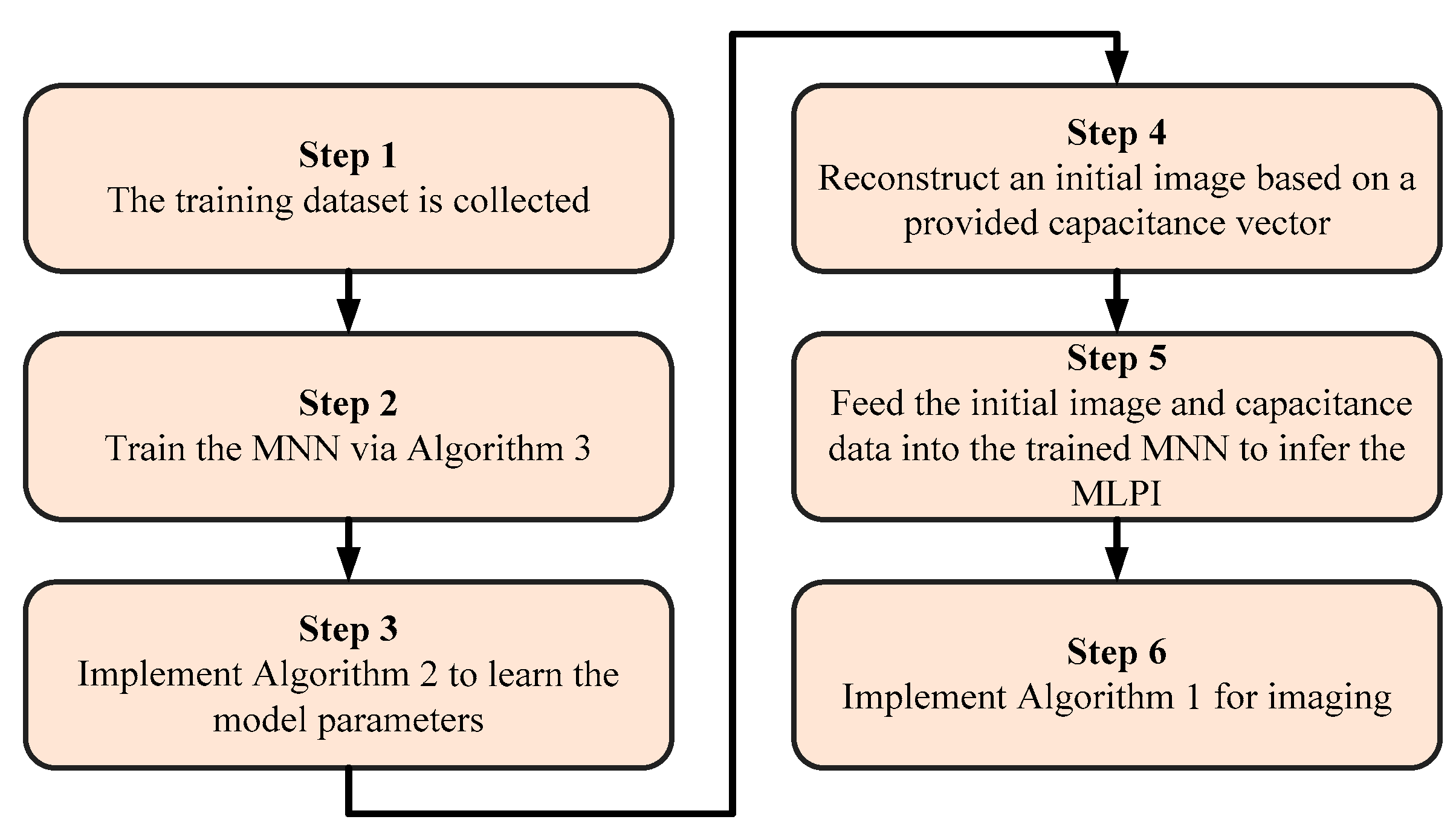
By integrating multi-objective optimization, bilevel optimization, robust optimization, measurement theory, and multimodal learning, our study proposes an innovative multi-objective robust optimization reconstruction (MOROR) algorithm. Its computational workflow is summarized in Figure 2.

The MOROR algorithm provides a comprehensive and systematic approach for image reconstruction. It integrates advanced machine learning techniques and multi-objective optimization methods to achieve high-quality reconstruction results. As shown in Figure 2, the implementation of the MOROR algorithm consists of six key stages, each providing crucial support for robust and efficient image reconstruction:

(1) Training sample collection. The collected training samples are used to train the MNN, ensuring that the algorithm has good generalization capabilities in various scenarios.

(2) Training the MNN using Algorithm 3. Based on the collected training samples, Algorithm 3 is executed to train the MNN. This step establishes a predictive model that serves as the core foundation for image reconstruction. The MNN can capture complex patterns and relationships in the data, thus providing accurate prior image predictions for subsequent stages.

(3) Determining the optimal configuration of model parameters using Algorithm 2. At this stage, Algorithm 2 is executed to determine the optimal configuration of model parameters. This step involves solving a multi-objective robust optimization problem to ensure the robustness and accuracy of image reconstruction under uncertain conditions.

(4) Initial image reconstruction using the newly acquired capacitance data. After determining the optimal model parameters, the initial image reconstruction is implemented using the newly acquired capacitance data. This step generates a preliminary image that serves as the input of the trained MNN.

(5) Inferring the MLPI using the trained MNN. The trained MNN is used for inferring the MLPI, a step that plays a pivotal role in enhancing reconstruction quality. This is because the MLPI serves a dual purpose: it not only acts as valuable prior knowledge that can be integrated into the reconstruction model but also functions as an effective initialization for iterative optimization processes. By providing a high-quality starting point, the MLPI significantly accelerates the convergence rate of optimization algorithms while simultaneously improving the accuracy and reliability of the final solution. Furthermore, the incorporation of the MLPI helps mitigate common reconstruction challenges such as noise amplification and artifact generation, particularly in ill-posed or underdetermined problems.

(6) Conducting final image reconstruction using Algorithm 1. In the final stage, the algorithm combines the newly acquired capacitance data with the inferred MLPI and the determined model parameters and completes the final image reconstruction by executing Algorithm 1.

In the MOROR algorithm, the first three steps (i.e., training sample collection, MNN training, and model parameter optimization) can be performed offline, meaning that they do not occupy time during the image reconstruction process. This offline processing enhances the algorithm’s efficiency, especially in applications with high real-time requirements. Once the MNN training is completed, its inference process is efficient, allowing the MLPI to be completed in a very short time. Since the MLPI inference time is extremely brief, its impact on the overall reconstruction time of the algorithm is negligible. The majority of the algorithm’s execution time is consumed by the operation of Algorithm 1, which is responsible for the final image reconstruction.

7. Validation and Discussion

We have analyzed and discussed the MOROR algorithm theoretically, and this section will focus on evaluating its advantages numerically by comparing it with well-known imaging algorithms.

7.1. Compared Algorithms and Implementation Details

Our analysis centers on a comparison of widely used iterative algorithms, as outlined in

Table 1. Tested algorithms.

Algorithms	Abbreviation
Polak–Ribière–Polyak conjugate gradient method [71,72]	PRPCG
Combined L1 with second-order total variation method [16]	L1SOTV
Joint L1 and total variation regularization [9]	L1TV
Elastic net regularization method [13]	ELNR
Transformed L1 regularization [73,74]	TL1R
L1/2 regularization method [75]	L1/2R
Joint L1 and low-rank regularization [8]	L1LR
L1 norm regularization method [76]	L1R
Low-rank regularization [77]	LRR
L1-2 regularization [5]	L1-2R
Fractional L1 regularization [19]	FL1R
Fractional-order elastic net regularization [18]	FOENR

. Since the MOROR algorithm is fundamentally iterative in nature, and non-iterative algorithms often fall short in achieving image reconstruction quality on par with iterative approaches, our evaluation is limited to iterative methods, excluding non-iterative algorithms from the comparison.

In Table 1, the PRPCG algorithm is a well-known unconstrained optimization algorithm and has a faster convergence rate than gradient optimization algorithms. The PRPCG algorithm is used on the premise that the objective function must be differentiable. The TL1R, L_1-2R, L1R, FL1R, and L_1/2R algorithms are renowned for their emphasis on leveraging the sparsity prior of imaging objects. The L1TV, L1SOTV, ELNR, FOENR, and L1LR algorithms are compound regularization methods. The LRR algorithm, renowned for its utilization of the nuclear norm to integrate the low-rank prior of imaging targets, represents a widely recognized approach in low-rank regularization methodologies. The algorithms selected for comparison are highly prevalent and have been extensively applied in the field of electrical capacitance tomography. Their extensive adoption establishes them as both credible and representative benchmarks for assessing performance. All the algorithms have been developed using the MATLAB R2021a platform.

In the NSGA-II algorithm, the number of populations is set to 20, and the maximum evolution generation is 150.

The MNN consists of an input layer, an output layer, and two hidden layers. The input layer takes capacitance signals and initially reconstructed images as input, with 1090 neurons. The output layer represents the true distribution of dielectric constants and has 1024 neurons. Each of the two hidden layers contains 2180 neurons, and their activation functions are sigmoid functions. To improve training stability, we have introduced two batch normalization layers. We use the Adam algorithm for training with an initial learning rate of 0.0001.

The imaging domain is discretized into 32 × 32-pixel elements, establishing a parameter space of a dimensionality of 1024. Within this framework, the dimensionality of the sensitivity matrix governing the physical model is 66 × 1024, while the acquired capacitance measurements constitute a vector with a dimensionality of 66 × 1.

7.2. Evaluation Criterion

In this study, we select two widely recognized metrics, namely image error and correlation coefficient, as standards for evaluating reconstruction quality [16].

Assessing the consistency of reconstruction results is equally important in determining the reliability of an algorithm. Therefore, we pay special attention to the performance stability of the MOROR algorithm under different operating conditions. To this end, we calculate the variance in the image error and correlation coefficient. A smaller variance indicates greater stability and consistency of the algorithm during the reconstruction process, thus enhancing its reliability in practical applications.

To comprehensively test the adaptability of the MOROR algorithm under different environmental conditions, we simulate various noise conditions and present visualized images under these conditions. At the same time, we provide the corresponding image error and correlation coefficient values to further analyze the algorithm’s performance in the presence of noise interference. This approach allows us to identify the algorithm’s potential and shortcomings in terms of noise resistance.

In designing the experiments, we refer to the definitions of noise levels in [16] to ensure the comparability and scientific validity of the results. Through such meticulous and comprehensive evaluation, we gain a more thorough understanding of the MOROR algorithm’s performance across diverse application scenarios while clarifying its advantages and areas for improvement. This provides valuable guidance for the further optimization of the algorithm and lays the foundation for its practical application.

7.3. Sensor Details

The inherent flexibility of capacitance sensors offers a wide range of layout possibilities, enabling their adaptation to various application scenarios. Among the available configurations, sensors with 12 electrodes are commonly considered optimal for achieving reliable performance across diverse use cases. In accordance with this widely accepted approach, our study also simulates a sensor configuration with 12 electrodes. Specifically, the sensing domain in these simulations measures 80 mm × 80 mm, aligning with previous work in the field [78]. This configuration is selected to ensure a balance between sensitivity, spatial resolution, and practicality, making it suitable for a broad spectrum of experimental and industrial applications.

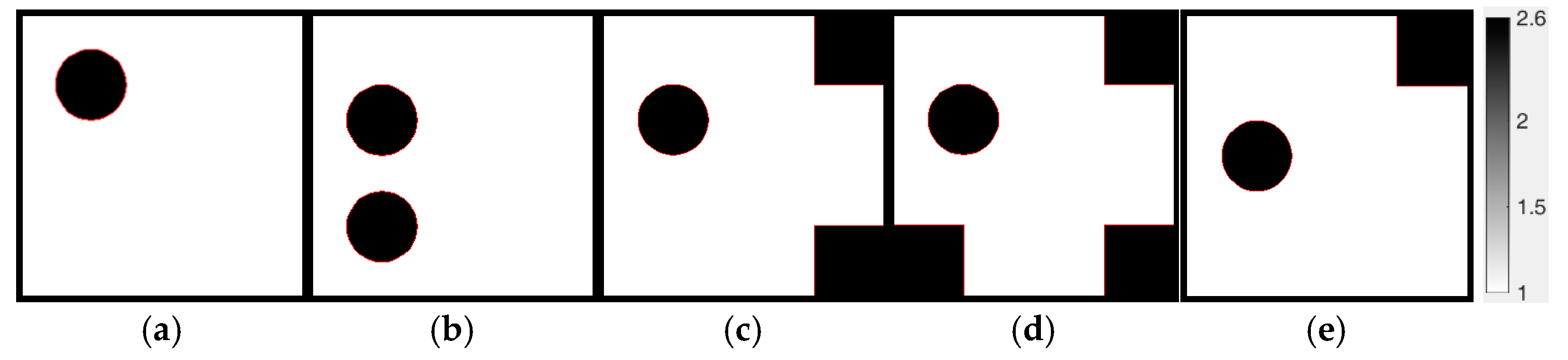
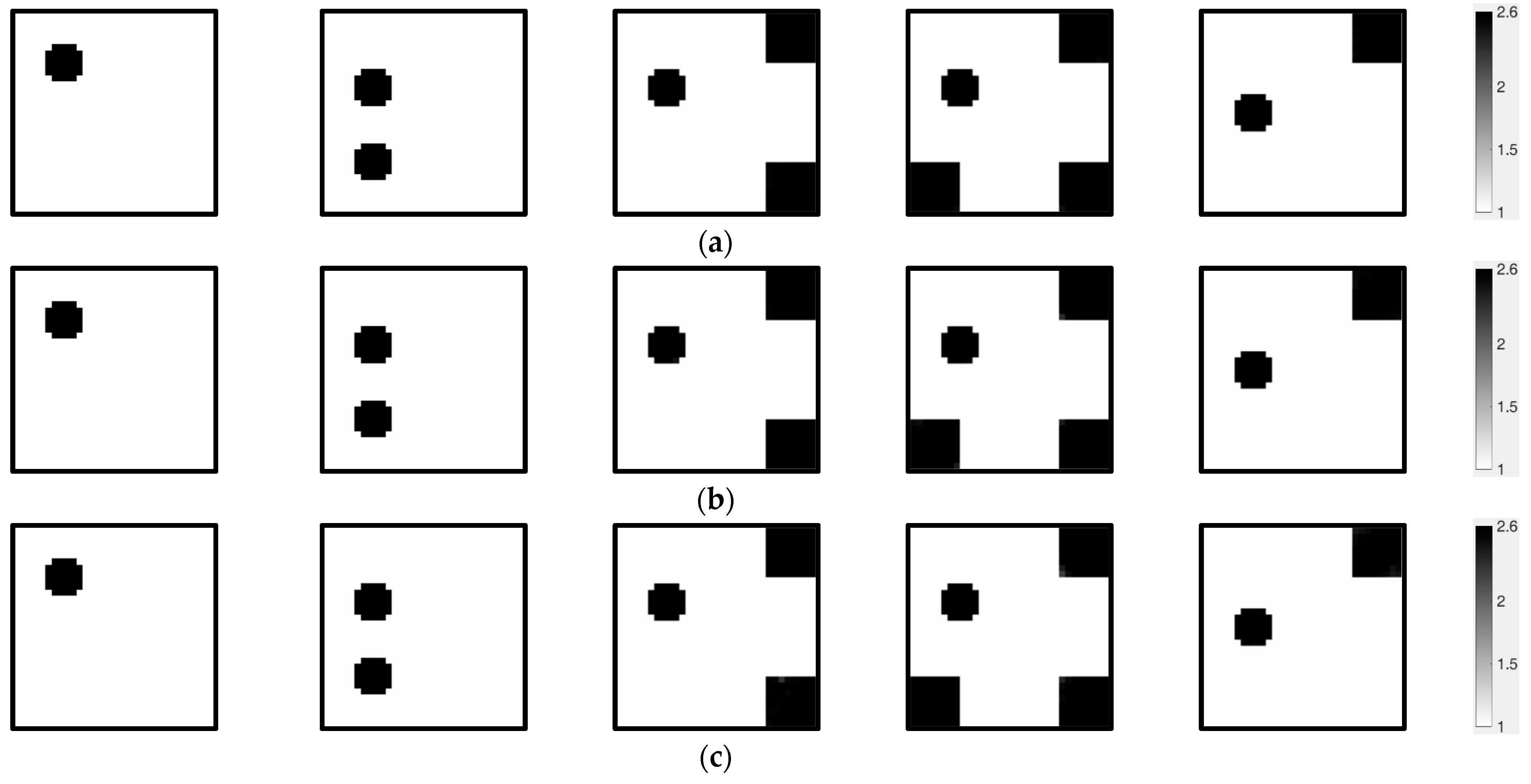
7.4. Reconstruction Objects

To evaluate the performance of our approach, we utilize the benchmark reconstruction objects in Figure 3. For simplicity, we will refer to Figure 3a through Figure 3e as reconstruction objects 1 through 5, respectively, in the following sections. These imaging objects are designed with black regions representing a high-permittivity medium and the remaining areas corresponding to a low-permittivity medium. The permittivity values for the high and low regions are set at 2.6 and 1.0, respectively. The geometric dimensions of these targets include circles with a 20 mm diameter and squares with 20 mm sides.

7.5. Results and Discussion

This section will present and analyze the reconstruction results, evaluate the noise resistance capabilities, and examine the imaging speed and stability of the reconstruction performance of the MOOR algorithm. These analyses aim to provide a comprehensive understanding of the algorithm’s practical applicability and reliability in real-world scenarios.

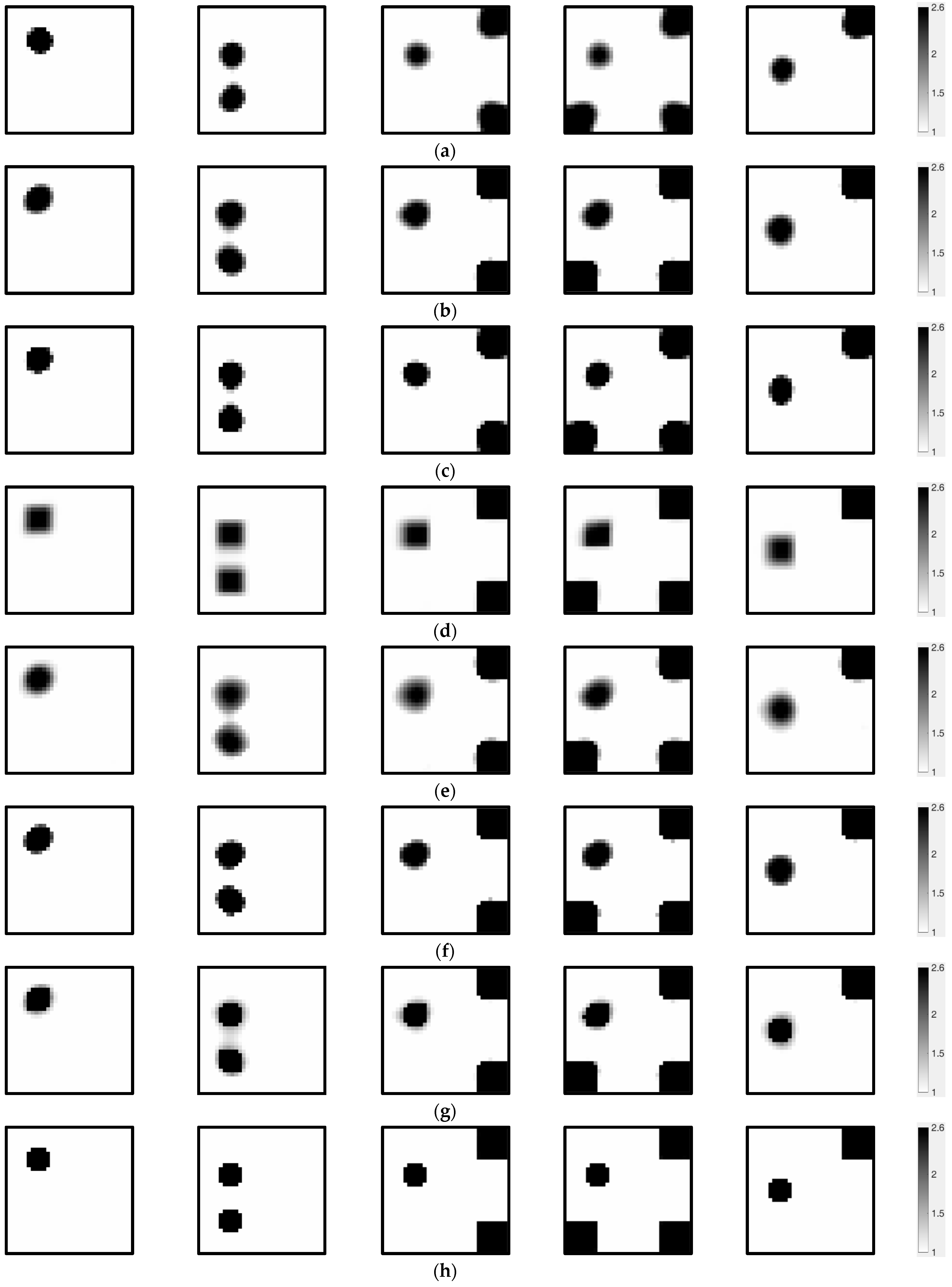
7.5.1. The Results of the Iterative Reconstruction Algorithms

The primary objective of this section is to conduct a comparison between the MOROR algorithm and iterative algorithms. We conduct an in-depth analysis of their performance across different reconstruction scenarios while systematically examining their respective strengths and limitations. The critical parameters used throughout the reconstruction procedure are delineated in

Table 2. The parameters of the compared iterative imaging algorithms.

Method	Parameter	Parameter Value
PRPCG	Step size	1
L1-2R	Regularization parameter	0.15
L1R	Regularization parameter	0.01
FL1R	Regularization parameter	0.09
LRR	Regularization parameter	0.01
L1/2R	Regularization parameter	0.02
TL1R	Regularization parameter	0.005

. The selection of these parameters not only affects the accuracy and efficiency of the algorithms but also plays a decisive role in determining the reconstruction quality. Through this comparative analysis, we gain enhanced insights into the applicability scope of each algorithm and identify potential optimization directions for future improvements. In the MOROR algorithm, the algorithm parameters are estimated by solving Equation (12) with $W_{ii}^{k+1}=1/(|u_i^k{|}^3+1e-10)$. The quantitative visualization results are illustrated in Figure 4, offering a clear graphical representation of the comparative performance of the algorithms. To ensure a more objective and comprehensive evaluation,

Table 3. Image errors of the compared iterative algorithms (%).

Method	Object 1	Object 2	Object 3	Object 4	Object 5
L1-2R	10.70	13.31	15.82	17.55	13.75
L1R	10.60	13.48	9.94	9.52	10.22
FL1R	9.44	11.41	10.43	11.14	10.97
LRR	11.78	15.16	9.45	8.30	10.93
PRPCG	11.24	16.88	11.92	10.64	11.62
L1/2R	12.14	16.13	10.23	10.40	10.89
TL1R	9.29	10.44	8.11	8.83	7.51
MOROR	0	0	0.26	0.39	0.16

and

Table 4. Correlation coefficients of the compared iterative algorithms.

Method	Object 1	Object 2	Object 3	Object 4	Object 5
L1-2R	0.9186	0.9175	0.9306	0.9229	0.9316
L1R	0.9221	0.9241	0.9722	0.9766	0.9633
FL1R	0.9381	0.9451	0.9690	0.9677	0.9568
LRR	0.8948	0.8970	0.9751	0.9825	0.9577
PRPCG	0.9050	0.8693	0.9598	0.9709	0.9520
L1/2R	0.9029	0.8984	0.9707	0.9721	0.9588
TL1R	0.9402	0.9549	0.9816	0.9800	0.9804
MOROR	1	1	1	1	1

provide detailed quantitative metrics, including image error and correlation coefficients. These metrics are critical for assessing the accuracy and consistency of the reconstruction results across different algorithms. By combining visual and quantitative analyses, we can identify the strengths and limitations of each algorithm, facilitating informed comparisons and highlighting areas for potential improvement.

From the results shown in Figure 4 and Table 3 and Table 4, it is evident that the algorithms being compared perform poorly in image reconstruction tasks and struggle to reconstruct high-quality images. In contrast, the MOROR algorithm performs excellently in image reconstruction tasks, achieving high-fidelity reconstruction. This conclusion is validated not only through subjective visual comparisons but also by the quantitative analysis results. The MOROR algorithm achieves a maximum image error as low as 0.39%, with a correlation coefficient peaking at 1. These numerical results clearly highlight the superior performance of the MOROR algorithm. Compared to existing reconstruction algorithms, the MOROR algorithm has made significant advancements in the design and solution of the reconstruction model and the exploration and integration of prior information, as well as the adaptive optimization of model parameters. The image reconstruction problem is modeled as a multi-objective robust optimization problem, which not only improves reconstruction accuracy and robustness but also provides a systematic reconstruction framework that facilitates parameter tuning and the optimization of reconstruction quality. In the MOROR algorithm, the LLOP integrates the MLPI, sparsity priors, and measurement principles, enhancing the diversity and complementarity of information in the reconstruction process, laying the foundation for reconstructing high-quality images. Specifically, the MLPI captures the statistical characteristics and patterns of the object to be reconstructed, not only integrating as a prior image into the reconstruction model, increasing the diversity and complementarity of prior information, but also serving as an ideal iterative initial value, improving the convergence of the algorithm. By integrating the MLPI, the fusion of measurement physics with multimodal learning is realized, contributing to a significant enhancement in reconstruction performance. The MOROR algorithm also realizes the adaptive selection of model parameters, facilitating the attainment of superior reconstruction results. Additionally, the adaptive learning of model parameters not only effectively eliminates the uncertainties caused by reliance on empirical selection methods, enhancing the model’s level of automation, but also significantly boosts the model’s ability to perform reconstruction tasks in complex environments.

We propose a new MNN to infer the MLPI. This new MNN performs inference tasks by simultaneously utilizing image and capacitance data. It fully leverages information from different modalities, compensating for the shortcomings of single-modality information and reducing potential information loss that may occur when only using one type of modality data, thereby improving the overall performance of the model. Notably, our proposed model can integrate any prior images, including inference information from any machine learning and deep learning methods, sensing information from other sensors, simulation information based on physical models, and more, without being limited to a specific type of algorithm. This enhances the model’s flexibility and adaptability. Moreover, we develop an efficient algorithm to solve the hierarchical multi-objective robust optimization problem. Both the visual results illustrated in Figure 4 and the quantitative data presented in Table 3 and Table 4 validate the efficacy of the introduced MNN and the newly designed optimizer.

Sparsity serves as a crucial prior in imaging, extensively utilized across numerous algorithms such as TL1R, L1R, FL1R, L_1-2R, and L_1/2R. This prior holds significant theoretical importance, helping algorithms to process image data more effectively and enhance image quality. However, extensive computational results indicate that in practical applications of electrical capacitance tomography, this prior information does not always perform well. For the reconstruction targets in Figure 3, we conduct a detailed comparative analysis of these reconstruction algorithms with different sparsity characteristics. The results show that the maximum image errors for these algorithms are 12.14%, 16.13%, 15.82%, 17.55%, and 13.75%, while the minimum correlation coefficients are 0.9029, 0.8984, 0.9306, 0.9229, and 0.9316, respectively. These data indicate that the quantitative image errors are substantial, rendering them incapable of precisely representing the spatial distribution of dielectric constants. This not only compromises the image quality but also leads to erroneous conclusions. In scenarios requiring high-precision reconstruction, these algorithms obviously cannot meet the demands. Although the sparsity prior has demonstrated certain advantages, there are still several issues in practical applications that need continuous research and improvement to meet the requirements of applications with high reconstruction precision.

The low-rank prior is another widely employed form of prior knowledge. The LRR algorithm incorporates the low-rank characteristics of the reconstruction target by utilizing the nuclear norm. It is difficult to fully characterize complex objects with the LRR method, and it tends to produce overly smooth solutions, making edges and subtle structures unclear. From the visual results in Figure 5d and the quantitative results provided in Table 3 and Table 4, it can be seen that the LRR algorithm cannot achieve high-quality reconstruction. For the reconstruction objects in Figure 3a–e, the image errors are 11.78%, 15.16%, 9.45%, 8.30%, and 10.93%, with correlation coefficients of 0.8948, 0.8970, 0.9751, 0.9825, and 0.9577, respectively. This result further underscores that relying exclusively on low-rank priors is inadequate for addressing intricate reconstruction challenges. Incorporating additional and more robust prior knowledge and enhancing the automation capabilities of models during the image reconstruction process can significantly enhance imaging quality. The effectiveness of the MOROR algorithm further validates this insight.

We also demonstrate the reconstruction results of the PRPCG algorithm. As seen in Figure 4e, this algorithm has certain limitations, posing challenges for achieving high-quality reconstruction. For the reconstruction objects in Figure 3, the PRPCG algorithm’s maximum image error reaches 16.88%, and the minimum correlation coefficient is 0.8693. In electrical capacitance tomography, leveraging prior information to improve reconstruction quality is essential. However, the PRPCG algorithm, being a gradient-based optimization algorithm, fails to incorporate such prior knowledge. Consequently, it falls short of reconstructing high-quality images. Enhancing the performance of the PRPCG algorithm requires additional research and development to align with the demands of real-world applications.

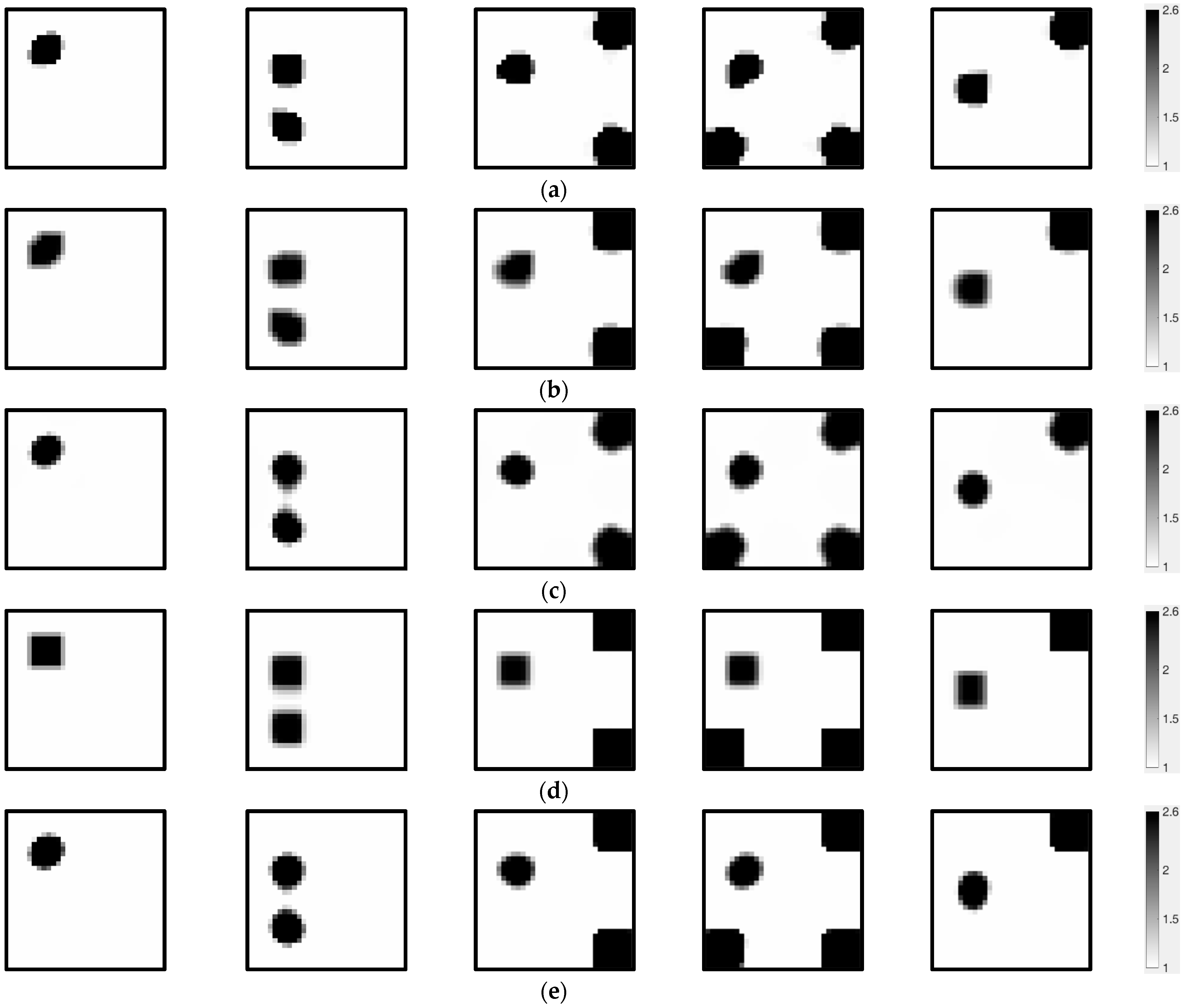
7.5.2. The Results of the Compound Regularization Algorithms

We compare the MOROR algorithm with five well-known compound regularization algorithms, including the L1TV method with the regularization parameters of 0.01 and 0.0003 for the L₁ norm and the total variation term, the L1SOTV method with the regularization parameters of 0.01 and 0.0008 for the L₁ norm and the second-order total variation term, the ELNR method with the regularization parameters of 0.02 and 0.003 for the L₁ norm and the L₂ norm, the L1LR method with the regularization parameters of 0.08 and 0.08 for the L₁ norm and the nuclear norm, and the FOENR algorithm with the regularization parameters of 0.0001 and 0.05 for the L₂ norm and the L₁ norm. Figure 5 displays quantitative visualization outcomes, offering an intuitive visual representation of algorithmic performance comparisons. For rigorous and unbiased assessment,

Table 5. Image errors of the compound regularization methods (%).

Algorithms	Object 1	Object 2	Object 3	Object 4	Object 5
L1TV	7.70	11.82	15.04	16.48	12.35
L1SOTV	11.59	14.86	9.90	10.01	9.42
ELNR	5.96	9.71	12.76	13.95	11.11
L1LR	12.29	13.94	7.95	7.39	10.17
FOENR	10.19	11.95	8.73	8.86	9.70

and

Table 6. Correlation coefficients of the compound regularization methods.

Algorithms	Object 1	Object 2	Object 3	Object 4	Object 5
L1TV	0.9576	0.9418	0.9352	0.9282	0.9454
L1SOTV	0.9028	0.9061	0.9726	0.9745	0.9689
ELNR	0.9729	0.9576	0.9536	0.9491	0.9555
L1LR	0.9014	0.9196	0.9822	0.9860	0.9632
FOENR	0.9291	0.9409	0.9785	0.9796	0.9672

summarize key numerical indicators, reconstruction errors and correlation metrics, which are critical for appraising the result precision and reliability across diverse methods. This dual analytical framework, merging qualitative and quantitative evaluations, allows the systematic identification of algorithmic advantages and limitations.

We compare the performance of several advanced compound regularization methods with the newly proposed MOROR algorithm. The results reveal the limitations of traditional compound regularization methods while highlighting the excellent performance of the MOROR algorithm in high-fidelity image reconstruction. By analyzing the data from Figure 5 and Table 5 and Table 6, we find that the five commonly used compound regularization methods struggle to achieve high-precision reconstruction for the targets shown in Figure 3a–e. The image errors for these methods range from 5.96% to 16.485%, while the correlation coefficients range from 0.9014 to 0.9860. These data indicate that despite these methods performing well in certain scenarios, they fall short when facing complex reconstruction tasks. In contrast, the MOROR algorithm demonstrates remarkable performance advantages. When handling the same reconstruction targets, the MOROR algorithm keeps the image error below 0.39% while maintaining a correlation coefficient of 1. This significant performance improvement is evident not only in quantitative metrics but also visibly through comparing the visual images in Figure 4 and Figure 5, where the superiority of the MOROR algorithm’s image quality is apparent.

Traditional compound regularization methods attempt to incorporate different priors by introducing regularization terms, but these methods rely on domain expert knowledge, making it difficult to fully and accurately capture the features of the reconstruction target. This has been confirmed by the visualization results in Figure 5 and the quantitative results in Table 5 and Table 6. Moreover, traditional methods depend on theoretical analysis or empirical adjustments for parameter configuration, resulting in low automation and difficulty adapting to complex and variable reconstruction tasks. In contrast, the MOROR algorithm integrates supervised learning and advanced optimization principles to achieve the automatic learning and optimization of model parameters, enhancing the algorithm’s level of automation.

7.5.3. Noise Sensitivity Assessment

Noise during the actual measurement process is unavoidable and has always been a major challenge for this measurement technology. Noise sensitivity limits the widespread application and further development of the technology. To address this challenge, we specifically introduce corresponding countermeasures in the design of the reconstruction model. In this section, we perform a comprehensive assessment of the robustness of the MOOR algorithm by analyzing capacitance data collected under varying noise conditions (5%, 10%, and 15%). The evaluation results are presented both qualitatively and quantitatively, with Figure 6 illustrating the visual reconstruction results and

Table 7. Image errors of the MOROR algorithm at different capacitance noise levels (%).

Noise Levels	Object 1	Object 2	Object 3	Object 4	Object 5
5%	0	0	0.28	0.46	0.27
10%	0	0	0.39	0.99	0.63
15%	0	0	0.91	1.21	1.14

and

Table 8. Correlation coefficients of the MOROR algorithm at different capacitance noise levels.

Noise Levels	Object 1	Object 2	Object 3	Object 4	Object 5
5%	1	1	1	0.9999	1
10%	1	1	1	0.9998	0.9999
15%	1	1	0.9998	0.9996	0.9996

providing statistical metrics, such as image error and correlation coefficients. This dual approach ensures a thorough understanding of the algorithm’s performance under noisy environments, highlighting its ability to maintain accuracy and consistency across different noise levels. By systematically evaluating its robustness, this analysis validates the algorithm’s potential for practical applications in real-world scenarios where noise interference is inevitable.

The precise reconstruction of images and the performance of algorithms in complex noise environments have always been central issues of concern in academia and engineering applications. Achieving high-precision and stable reconstruction in complex noise scenarios is not only directly related to the practicality and reliability of this technology but also holds significant implications for technological developments in related fields. As shown in Figure 6 and Table 7 and Table 8, the MOROR algorithm demonstrates outstanding performance advantages under different noise conditions, consistently maintaining image errors at a relatively low level. Specifically, the maximum image error of the MOROR algorithm is only 1.21%, while the minimum correlation coefficient is 0.9996. This fully proves the robustness and superior performance of the algorithm in noisy environments.

The exceptional robustness of the MOROR algorithm is attributed to several key features and innovative designs. Firstly, the MOROR algorithm introduces a multi-objective robust imaging model that reduces sensitivity to noise during the image reconstruction process. This model considers the balance between imaging accuracy and algorithm robustness, allowing the algorithm to maintain stable performance in various noise scenarios. Secondly, the MOROR algorithm incorporates regularization techniques and integrates multiple types of prior information. The enhancement in the diversity and complementarity of prior information helps improve imaging quality and the robustness of the algorithm. Additionally, the use of regularization techniques effectively mitigates the interference of measurement noise. Thirdly, the MOROR algorithm has the capability to automatically calculate model parameters. Compared to traditional algorithms that rely on manual adjustments, this adaptive optimization strategy significantly improves the model’s adaptability and reconstruction quality in complex and high-noise scenarios.

7.5.4. Reconstruction Time

In the research and application of iterative algorithms, imaging time is one of the core metrics for evaluating algorithm performance. This is especially true in dynamic, rapidly changing scenarios where the importance of imaging speed is more pronounced. For these scenarios, measurement technologies need to have high-speed and real-time data processing capabilities to meet the stringent response speed requirements of practical applications.

In the reconstruction tasks shown in Figure 3a–e, the MOROR algorithm’s reconstruction times are approximately 0.0472 s, 0.0414 s, 0.0442 s, 0.0449 s, and 0.0433 s, respectively, showing fairly consistent and fast reconstruction capability. While certain algorithms may achieve shorter reconstruction times compared to the MOOR algorithm, their reconstruction quality is notably inferior. A meaningful comparison of reconstruction times can only be made when the quality of the reconstructions is on par.

The reconstruction time of the MOROR algorithm is mainly spent on solving the LLOP. This is because the algorithm is designed to offload other computational tasks such as model training and model parameter learning as much as possible, concentrating more computing resources on the online reconstruction process. However, despite the MOROR’s simplified iterative structure, its iterative nature still poses challenges to real-time imaging. These challenges arise from the inherent conflict between two competing objectives: increasing the reconstruction speed and reducing the reconstruction error. Effectively balancing these two objectives remains an unresolved challenge in the field of iterative algorithms, and this limitation also hinders the broader adoption of electrical capacitance tomography technology in real-world industrial and scientific applications. The real-time imaging demands of rapidly changing scenes intensify this contradiction, making it difficult for traditional methods to maintain both accuracy and efficient computational performance.

Enhancing the reconstruction speed typically involves simplifying models or decreasing the number of iterations, which can compromise accuracy. On the other hand, striving for high accuracy often results in greater computational complexity and longer processing times. This inherent conflict is one of common obstacles faced by iterative algorithms and is a core challenge that the MOROR algorithm needs to address in further optimization. There is still room for optimization in the MOROR algorithm. Future research will focus on developing more efficient solving strategies to shorten the reconstruction time.

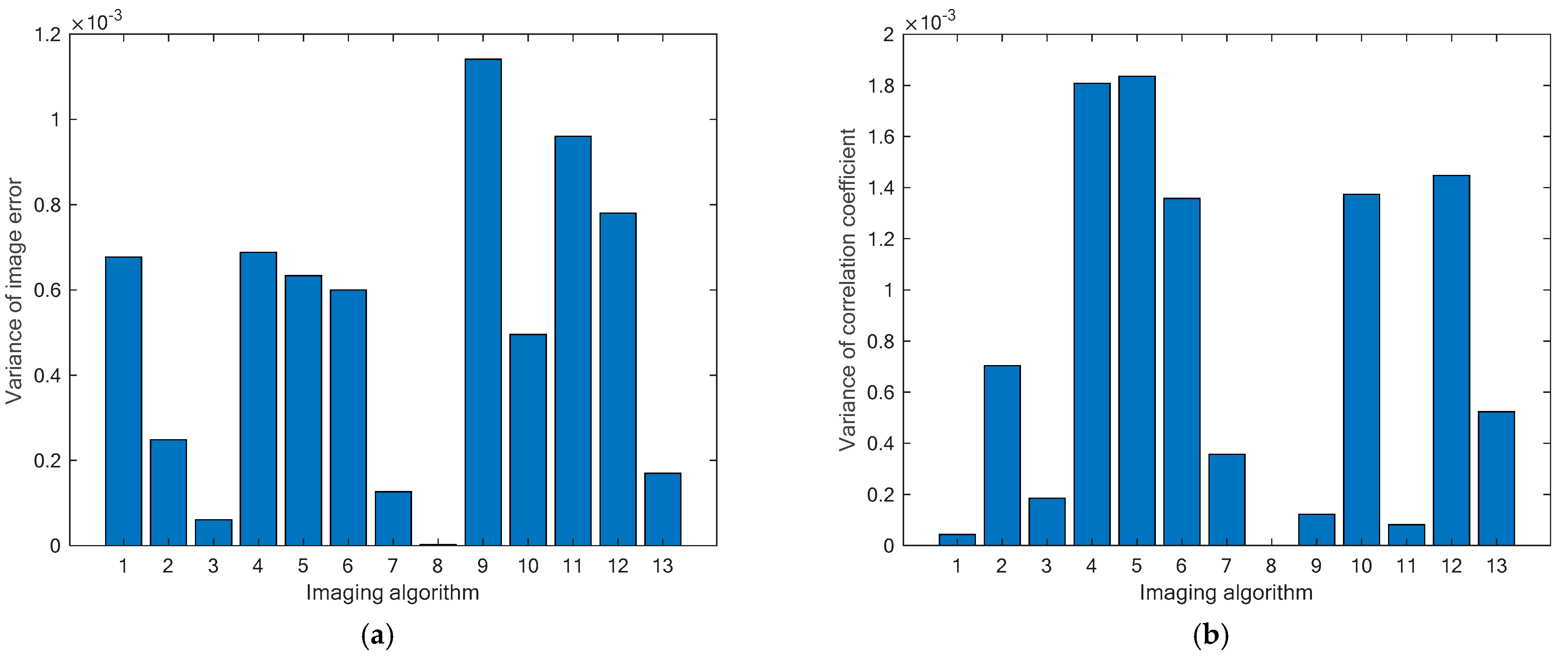
7.5.5. Consistency of Reconstruction Performance

In this section, we systematically evaluate the stability of the MOROR algorithm by analyzing the variance in the image error and correlation coefficients, with the quantitative results shown in Figure 7. These indicators quantify the consistency of the algorithm across different reconstruction tasks. To further validate the analysis results, Figure 8 demonstrates the performance of different algorithms in terms of the image error and correlation coefficients under various reconstruction objects. These quantitative results lay a foundation for a thorough comparison between the performance of the MOROR algorithm and that of other methods, which supports the subsequent optimization of these algorithms.

By analyzing the data visualization results in Figure 7, it can be seen that among all the algorithms evaluated, the MOROR algorithm exhibits significant advantages across multiple dimensions. In particular, the MOROR algorithm achieves the lowest values in the two critical performance indicators, i.e., the variances in image errors and correlation coefficients, far surpassing other algorithms. This result fully demonstrates the exceptional stability and effectiveness of the MOROR algorithm in image reconstruction tasks, indicating its ability to consistently maintain high-quality reconstruction results while handling complex tasks with excellent robustness.

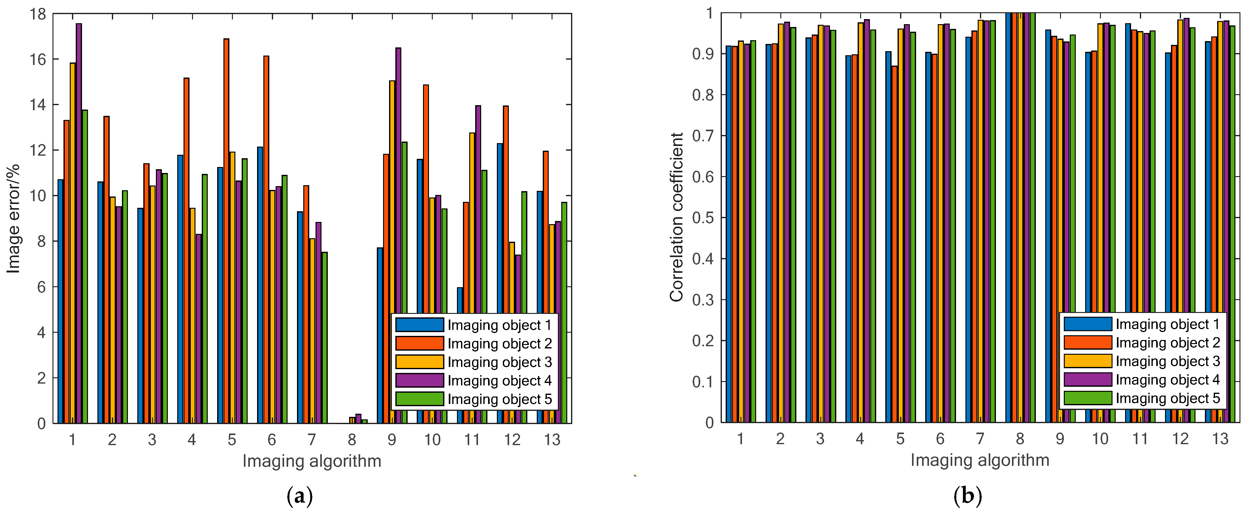
To delve deeper into the specific performance of each algorithm across various reconstruction tasks, Figure 8 illustrates the image errors and correlation coefficients of different algorithms in a range of reconstruction objects. Despite minor variations in the image errors and correlation coefficients across different reconstruction targets, the MOROR algorithm demonstrates consistently stable performance, exhibiting a narrower range of performance fluctuations and maintaining consistently low error levels. This indicates that the performance of the MOROR algorithm is less related to task characteristics, exhibiting stronger adaptability and performance consistency.

8. Conclusions

This study proposes an innovative multi-objective robust optimization method to alleviate the technical bottleneck caused by low imaging quality. This new approach integrates advanced optimization principles, multimodal learning, and measurement physics to alleviate reconstruction challenges under complex and uncertain conditions, achieving excellent reconstruction performance. It consists of two mutually nested and dependent optimization problems, the ULOP and the LLOP, which can simultaneously achieve the automatic tuning of model parameters and the optimization of reconstruction quality. A new LLOP is derived using the regularization theory to unify the MLPI, sparsity prior, and measurement physics into an optimization framework. To enhance the inference accuracy of the MLPI, we design the MNN, which improves the model’s inference ability through the fusion of multimodal information. To mitigate the computational difficulties induced by the ULOP-LLOP interdependencies, an innovative nested algorithm is proposed to solve the proposed multi-objective robust optimization model. The evaluation results indicate that the proposed method exhibits significant advantages over existing mainstream imaging algorithms. It enhances the automation level of the image reconstruction process, improves imaging quality, and demonstrates excellent robustness. For the studied reconstruction objects, the maximum image error is 0.39%, and the minimum correlation coefficient is 1 when capacitance noise is not considered. When the capacitance noise is 15%, the maximum image error increases to 1.21%, and the minimum correlation coefficient is 0.9996. Furthermore, the novel algorithm demonstrates remarkable stability in performance, maintaining consistent reconstruction quality without substantial fluctuations across varying reconstruction targets. This research not only provides a comprehensive method to improve the overall performance metrics of image reconstruction but also establishes a new imaging paradigm, which is expected to accelerate the expansion of this measurement technology’s application boundaries.

Despite numerous advantages and potential of multi-objective optimization, robust optimization, and bilevel optimization, they have not been sufficiently studied and explored in the field of electrical capacitance tomography, limiting the innovative development of imaging algorithms and hindering further improvements in the technology’s accuracy, efficiency, and adaptability. Our work aims to overcome this bottleneck and promote the innovative development of reconstruction algorithms. Future research will focus on developing more advanced modeling methods to enhance the automation of the image reconstruction process, strengthen adaptability in complex reconstruction scenarios, and substantially improve the intelligence level of measurement equipment.