Application of Image Recognition Methods to Determine Land Use Classes

Featured Application

Documenting alterations in land use over a specified duration.

Abstract

The increasing availability of satellite data and advances in machine learning (ML) have significantly enhanced land use image classification for environmental monitoring. However, the primary challenge in land use classification using satellite imagery lies in the presence of cloud cover, variations in data resolution, and seasonal changes, which impact classification accuracy and reliability. This paper aims to improve the assessment of land cover changes by proposing a hybrid ML, cloud interpolation, and vegetation indices-based approach. The proposed approach was implemented by using a random forest (RF) classifier, combined with cloud interpolation and vegetation indices, to classify land use Sentinel-2 satellite imagery in the Baltic States. The experimental results demonstrate that the proposed approach achieves an accuracy rate above 90%, effectively demonstrating its capacity to distinguish between various land use types. We believe that this study and its results will inspire researchers and practitioners to further work towards land use classification by applying ML algorithms and offer valuable insights for future classification tasks involving noise digitalization and research.

1. Introduction

The rapid expansion of remote sensing technologies and the increasing availability of high-resolution satellite data have made it essential to efficiently monitor and manage land resources. However, land use classification remains a complex problem due to the variability in spectral characteristics, seasonal changes, and cloud interference that often obscure satellite images [1,2]. Traditional classification methods in dynamic environments [1] highlight the need for advanced methodologies that utilize artificial intelligence techniques [2,3].

Some existing research has already tried to solve the problem of land use classification. Our comprehensive review of related works indicates that the primary algorithm used by researchers is random forest (RF), although other algorithms have seen increased usage in recent years. For instance, authors [4] investigated RF for vegetation mapping in Northern Croatia, integrating Sentinel-1 SAR and Sentinel-2 satellite imagery data. Their findings confirmed that the fusion of SAR and optical indices, such as the normalized difference vegetation index (NDVI) and texture features, significantly improved classification accuracy, achieving an overall accuracy of 91.78%. Similarly, the authors of [5] used RF with object-oriented classification to address the “salt-and-pepper” effect in crop classification, achieving an outstanding accuracy of 98.66% and a kappa coefficient of 0.9823. Furthermore, the authors [6] demonstrated the applicability of RF in large-scale land cover classification by leveraging segmentation models in remote sensing imagery analysis. In [7], the authors investigated cropland and crop type classification in Ethiopia, highlighting the potential of integrating Sentinel-1 and Sentinel-2 time-series data within Google Earth Engine. The study demonstrates that RF remains highly effective when applied to large-scale agricultural monitoring, achieving remarkable classification accuracy. Additionally, the authors of [8] have employed RF with multi-temporal RADARSAT (a Canadian remote sensing Earth observation satellite program) constellation mission data, demonstrating its ability to improve crop classification performance. In [9], the authors extended the applicability of RF to coastal wetland vegetation classification, reinforcing its versatility across various ecosystems. These studies collectively emphasize the continued relevance and superiority of RF in remote sensing applications, positioning these authors as leading contributors to the field.

However, the majority of land use classification studies focus on the classification of the territory under consideration. In many cases, these models are unable to be dynamically adapted independently of the input satellite data provided. Furthermore, it has been observed that solutions to the cloud problem, which is of significant importance when classifying territories such as the Baltic region, are not always distinguished in data preparation [10].

This paper aims to enhance the evaluation of land cover changes by proposing a hybrid machine learning (ML), cloud interpolation [11], and vegetation indices-based approach. This study specifically focuses on developing a robust classification pipeline that incorporates pre-processing techniques such as cloud interpolation, spectral index calculations, and an ML-based classification approach using the Random Forest algorithm [12]. The proposed method is tested on the territory of Lithuania, where diverse land use classes, seasonal variations, and frequent cloud cover pose significant challenges to classification accuracy.

The main contribution and novelty of this research are as follows:

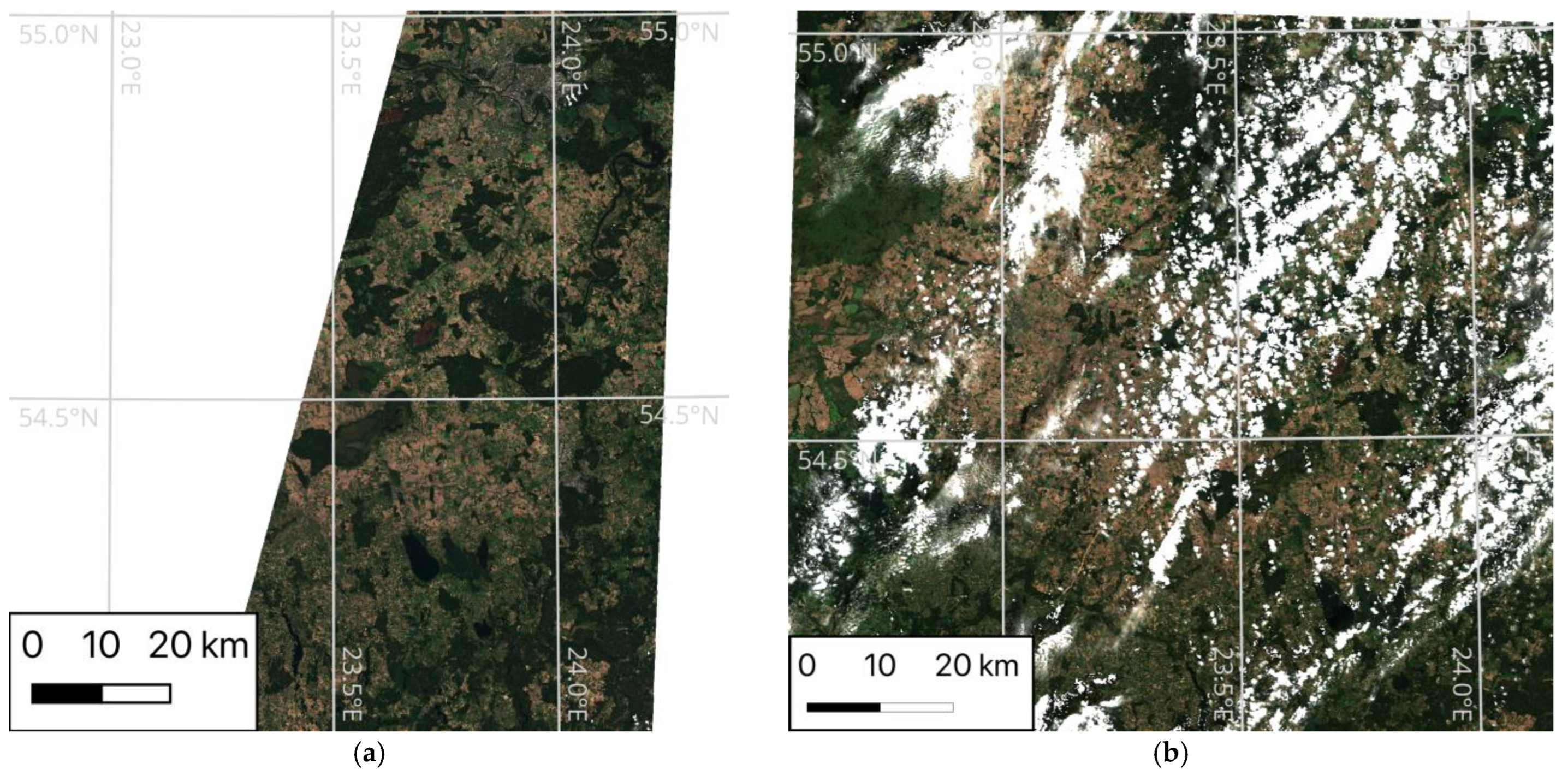
• An enhanced data pre-processing workflow is presented, demonstrating a substantial improvement in classification performance through effective management of cloud-covered satellite images.
• An advanced feature selection strategy using vegetation indices to improve class separability was employed.
• A post-processing approach that utilizes confidence maps to refine classification results and reduce misclassification errors was proposed.
• The results of experiments performed on the territory of Lithuania demonstrated a substantial enhancement in classification accuracy, taking into account the diverse land use classes, seasonal variations, and frequent cloud cover present in the region.

The remainder of the paper is organized as follows. Section 2 (Related Works) provides a detailed review of recent studies employing ML algorithms for land cover classification, emphasizing the effectiveness of the Random Forest algorithm in various scenarios. Section 3 (Methodology) describes the hybrid approach proposed for classifying land use with Sentinel-2 imagery. This section is subdivided into data acquisition, preprocessing, classification, and post-processing phases, detailing each step in the pipeline. Section 4 (Experimental Results) presents the outcomes of applying the proposed methodology to Sentinel-2 data covering Lithuania. Section 5 (Discussion) analyses the results, discussing the effectiveness of the approach and its limitations. Section 6 (Conclusions and Future Works) summarizes the key findings and contributions of the study.

2. Related Works

The application of ML algorithms in remote sensing has gained considerable momentum. Researchers are focusing on various aspects of land cover and landscape pattern analysis to address ecological and urban development issues. Recent studies highlight the versatility and robustness of these algorithms in dealing with complex spatial data across diverse environments. The following analysis examines relevant related research on land cover classification.

Sentinel-2 satellite imagery has demonstrated superior performance for land use and land cover mapping in the northern Congo Republic, achieving higher overall accuracy (93.80%) and Kappa coefficient (0.89) compared to Landsat 9 (91.60% accuracy, Kappa 0.85) [13]. Additionally, Sentinel-2 imagery surpassed Landsat-9 in terms of spatial resolution, effectively mitigating the issue of mixed pixels. It also demonstrated a stronger alignment with in situ spectral measurements during local field comparisons [14]. Sentinel-2 imagery has been shown to have a clear advantage over Landsat imagery for snow cover detection due to its higher spatial and temporal resolution, which enables the better monitoring of snow dynamics, especially in mountainous regions like Switzerland [15].

The authors of [16] used the Random Forest (RF) algorithm to analyze land fragmentation in Nice, France. They used metrics like mean fragment size, core area, and contrast index. They strategically used pre-processed, cloud-free Sentinel-2 images to ensure high data quality, which is crucial for achieving reliable classification results. This study highlights the importance of high-quality, clean datasets in environmental monitoring and the effectiveness of RF in extracting meaningful landscape patterns.

In contrast, the authors [4] addressed the challenge of cloud coverage in remote sensing by integrating Sentinel-1 synthetic-aperture radar (SAR) and Sentinel-2 optical data in their analysis of Northern Croatia. Their approach utilized the RF algorithm and demonstrated the potential of multi-sensor data fusion in enhancing land cover classification under less-than-ideal conditions. The use of overall accuracy (OA) and Cohen’s Kappa (CK) as performance metrics provided a quantitative assessment of the method’s efficacy, illustrating the hybrid approach’s advantage in cloud-prone areas.

The authors of [5] explored the effectiveness of combining Random Forest (RF) and Support Vector Machines (SVM) in Inner Mongolia, expanding the scope of algorithm application. This dual-algorithm approach sought to leverage the strengths of both RF and SVM, with a particular focus on enhancing the robustness of the classification process under varied environmental conditions. Their innovative use of object-oriented methods to mitigate disturbances from cloud cover represents a significant step forward in preprocessing techniques, potentially setting a new standard for handling optical data distortions in remote sensing.

Cloud interpolation is a critical process in remote sensing, addressing data gaps in satellite imagery caused by cloud cover [11,17]. Recent advancements have introduced innovative methods to enhance the accuracy of reconstructing these obscured areas. One such approach is the spatial-spectral random forest (SSRF), which utilizes spatially adjacent and spectrally similar pixels to fill gaps, effectively removing thick clouds by leveraging spatial and spectral information simultaneously [18]. Another significant development is the integration of deep learning techniques, such as partial convolution within a U-Net architecture. This approach has shown significant improvements in interpolating land surface temperature data by considering local ground-site air temperature measurements, leading to a 44% reduction in root mean square error compared to traditional methods. These advancements highlight the continuous improvement of cloud interpolation techniques, enhancing the reliability of satellite-derived datasets for environmental monitoring and analysis [19,20,21].

For a more comprehensive overview of the methods and outcomes used in various studies employing ML algorithms in remote sensing, some relevant related works are compared below in

Table 1. Comparison of the related works found on land use classification (Random Forest (RF), Support Vector Machine (SVM), Deep Convolutional Neural Networks (DCNN), NDVI-based ML (NDVIML), Convolutional Neural Networks (CNN), Overall Accuracy (OA), Cohen’s Kappa (CK), Precision (P), Recall (R), F1-score (F1), Global Accuracy (GA), Multi-Scale Convolutional Neural Network (MSCNN), Object-Based Image Analysis with Fuzzy Logic (OBIAFL), Vector Space Model (VSM), Gradient Boosted Machine (GBM), XGBoost (XBG), Classification and Regression Tree (CART), Lasso Regression (LR)).

Reference	Algorithm	Accuracy Metrics	Analyzed Region	Cloud Problem Handling
(1)	(2)	(3)	(4)	(5)
[16]	RF	OA = 74.3%	Nice, France	Used pre-processed cloud-free Sentinel-2 images
[4]	RF	OA = 91.78%	Northern Croatia	Used Sentinel-1 SAR and Sentinel-2 optical data, applied cloud masking strategies
[5]	RF, SVM	OA = 98.66%, CK = 98.23%	Inner Mongolia	Applied object-oriented methods to mitigate noise, no specific mention of cloud handling
[7]	RF	OA = 88.18%, P = 93.55%, R = 89.93%, F = 91.67%	Ethiopia	Multi-temporal cloud-free compositing approach
[9]	RF	OA = 95.64%, CK = 94%	Yancheng, China	Sentinel-2 cloud masking and shadow removal techniques
[8]	RF	OA = 91.2%, CK = 85%, F1 = 91.04%	Various crop fields	Multi-temporal imagery for cloud interpolation
[22]	CNN	F1 = 75.49%	Global	Used deep learning for cloud detection and mitigation in high-resolution images
[23]	RF	OA = 94.78%, F1 = 78.32%	Flood-prone areas	Combined cloud-free mosaicking with SAR data
[24]	RF	OA = 91.46%	Canada	Scene Classification Layer (SCL) for cloud segmentation
[25]	NDVIML	OA = 83.75%	Agroforestry areas	Cloud filtering via NDVI-based thresholding
[6]	RF, CNN	OA = 90.3%	Remote sensing datasets	Combination of cloud masking and deep learning interpolation
[26]	CNN	GA = 88%	Manitoba, Canada	Not specified
[27]	SVM, RF	OA = 86%	Krakow, Poland	Sentinel-2 imagery pre-processing; addressed cloud interference implicitly
[28]	RF	OA = 88.16%	Lingbei Rare Earth Mining Area, China	Not explicitly mentioned (hyperspectral data used, which is generally less affected by cloud issues than optical data)
[29]	OBIAFL	OA = 95.32%	Pavia, Italy	Not specified
[30]	VSM	Not specified	Coastal zones in California, USA	Not specified
[31]	GBM, RF	OA = 87%	Queensland, Australia	Explicitly addresses cloud issue; RF efficiently interpolates missing pixels caused by clouds
[32]	KNN, DT, SVM, RF	OA = 81%	Algarve, Portugal	Uses good quality pre-processed Sentinel-2 Level-2A products
[33]	SVM, RF	F1 = 91.4%	Bulgaria	Uses images with cloud cover <10% and apply cloud, shadows and defective pixel masking
[34]	RF, SVM, XGB	OA = 83–96% F1= 73–97%	Tatra Mountains, Central Europe	Authors use high quality Sentinel-2 Level-2A products
[35]	RF, SVM	F1 = 93%	Tatra Mountains, Central Europe	Selects only those Sentinel-2 Level-2A scenes that exhibit minimal cloud cover
[36]	KNN, SVM, DT, RF	CK = 87%	Central Iran	Cloudy images omitted (dry climate)
[37]	RF, KNN	R2 = 87%	Central Greece	Cloud masking
[38]	KNN, SVM, RF	OA = 86–93%	China	Not specified
[39]	RF, SVM, DT, CART	OA = 94.8%, CK = 93%	Nainital, India	Authors use Google Earth Engine (GEE) for cloud free images
[40]	SVM, RF	OA = 90.11%, CK = 87%, F1 = 88.46%	Catalonia	Authors handle cloud problems in their analysis by using atmospheric and geometric corrections
[41]	SVM, RF, KNN, LR	R2 = 79%	Jilin Province, Northeast China	Sen2Cor tool applied
[42]	RF, SVM	OA = 94.03%,	Lake Basin, Iran	Not specified
[43]	RF, CART	R2 = 94.1%	Romania	Authors use Google Earth Engine (GEE) for cloud free images
[44]	RF	OA = 87.15%	Central Italy	Cloud masking

. This table provides a comparison of the algorithms used, the accuracy metrics evaluated, and strategies for handling cloud interference across different geographical regions, offering readers an expanded perspective on the field’s current research trends. In cases where two or more algorithms are considered, the “Accuracy metrics” column shows the best result obtained (see Column 1 in Table 1). When one or more algorithms are considered in different situations, the accuracy result is presented by calculating the average (see Column 1 in Table 1).

Summing up, the results of Table 1 indicate that the most frequently used algorithm for land use classification is Random Forest (RF) (found in 25 papers of the 30 analyzed papers (see Column 2 in Table 1)). It is also noteworthy that in the majority of cases (see Column 5 in Table 1), satellite data processing techniques are described. For instance, in [1,8,9,45], these techniques are addressed in a variety of ways in the context of the cloud problem. Despite the utilization of disparate data processing and accuracy measurement metrics, the selection of metrics was found to be dynamic. For example, the Overall Accuracy metric was the most frequently used [6,8,16,23,27,28,45], and similarly, Cohen’s Kappa [5,9,22,39,40] or F1-score [1,8,23,34] were viable options for verifying the results (see Column 3 in Table 1). It is also noteworthy that the accuracy results achieved by the articles examined in the literature analysis are indeed dynamic (see Column 3 in Table 1). This distribution can be attributed to various factors, including differing research objectives, satellite utilization as input data, and different combinations of classified classes. It is also noteworthy that the geographical locations of the study sites are distributed across the globe, with a significant presence in multiple regions (see Column 4 Table 1).

To conclude, further research is necessary to apply the ML algorithms identified in other studies to various types of input data, such as Sentinel-2 satellite imagery of different geographical regions, and to measure the accuracy of the results using different metrics. Extensive research involving various algorithms and input data from different regions has provided us with a more comprehensive global perspective on the accuracy and characteristics of these ML algorithms when processing regional input data. Moreover, different insights for the further classification of different regions will be obtained.

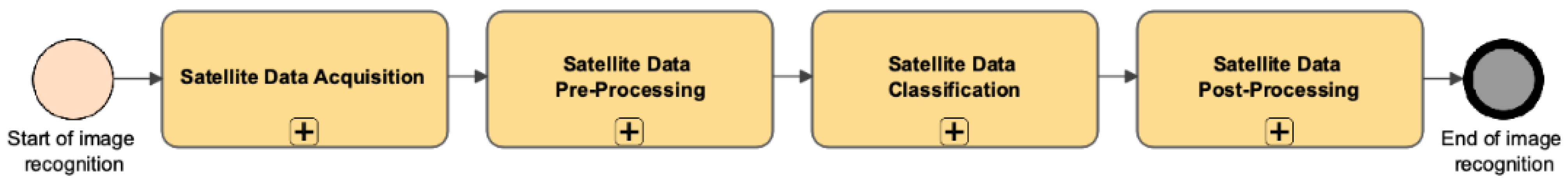
3. Materials and Methods

This section presents the proposed hybrid ML, cloud interpolation, and vegetation indices-based approach for the classification of Sentinel-2 satellite imagery. The methodology is structured into three main components—data acquisition, pre-processing, and classification—followed by post-processing (see Figure 1). Data acquisition involves retrieving Sentinel-2 satellite images and filtering them based on cloud cover and resolution criteria. Pre-processing steps focus on preparing the data for analysis, including image merging, cloud removal, and spectral index calculations to enhance feature representation. The classification stage utilizes a random forest (RF) model to assign land use labels, leveraging training datasets constructed from accurately labeled reference data. Finally, post-processing techniques are then applied to refine classification results by filtering out low-confidence predictions and improving spatial consistency [46]. These methodological components work together to enhance the reliability and precision of the classification outcomes.

Below, the description of each sub-process denoted by a plus symbol (+) in Figure 1 is presented.

3.1. Satellite Data Acquisition

The first step in our methodology involves obtaining Sentinel-2 satellite imagery. Sentinel-2, which is managed by the European Space Agency (ESA), provides multi-spectral data with resolutions ranging from 10 m to 60 m. To ensure high classification accuracy, we utilized Level-2A data, which are atmospherically corrected and pre-processed to reduce noise. The study focused on the territory of Lithuania, where Sentinel-2 data were retrieved from 2022 to 2024. Strict filtering criteria were applied to enhance the quality of data used for classification, ensuring that only images with cloud coverage below 20% were selected. This choice of threshold is supported by previous research findings that have shown that images with less than 20% cloud cover provide an optimal balance between data quality and availability (especially for model training), thereby minimizing spectral distortions or potential errors in the training sets. It is strongly recommended that cloud contamination be limited to this level to ensure the reliability and accuracy of analyses in land use remote sensing applications.

Additionally, metadata such as acquisition time, sensor angle, and cloud masks were analyzed to identify the most suitable images for classification. The detailed data acquisition schema is presented in Figure 2.

As shown in Figure 2, Figure 3 provides a detailed representation of the satellite data download process.

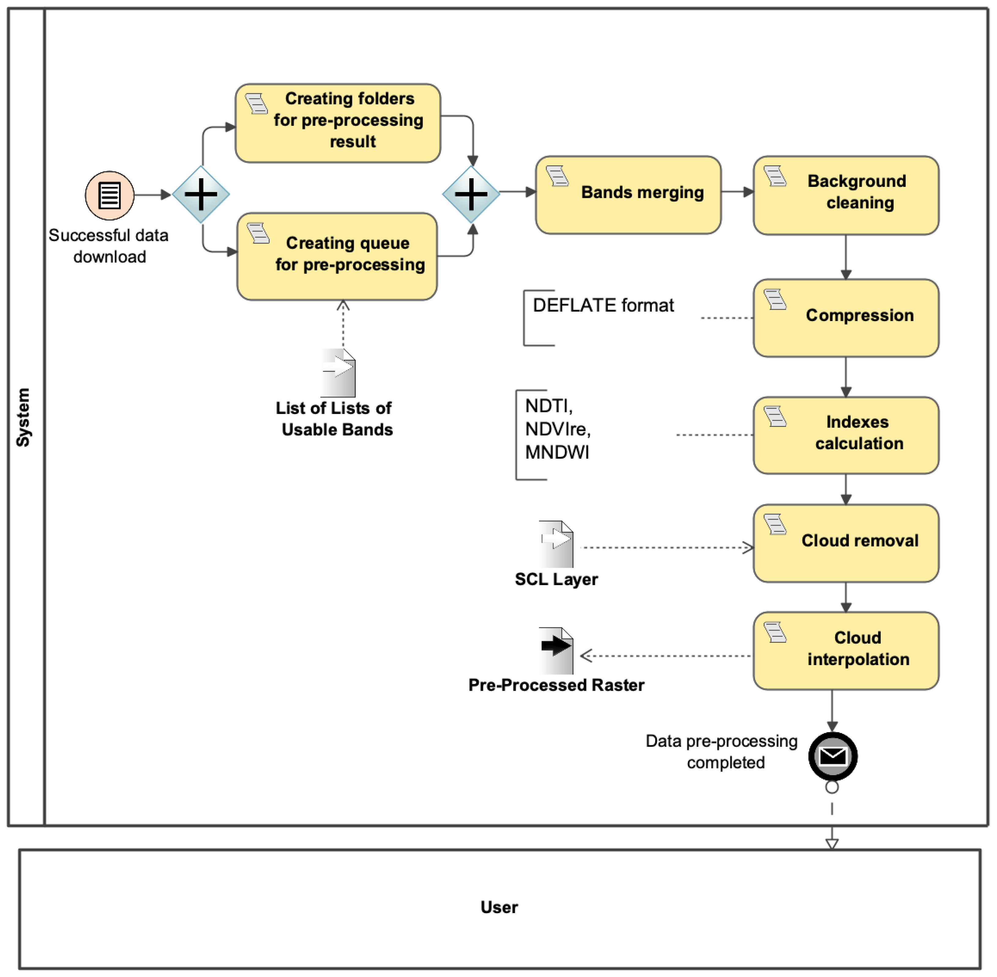
3.2. Satellite Data Pre-Processing

Pre-processing is a crucial stage in preparing satellite data for classification. Several operations were applied to enhance the quality of the images:

• Image Merging: Sentinel-2 bands were combined into a single multi-band image for comprehensive spectral analysis [6,47,48,49].
• Background Cleaning: NoData pixels and irrelevant background noise were removed using a thresholding approach [50,51].
• Compression: The lossless DEFLATE type compression method was applied to pre-processed photos to save memory resources [52,53,54].
• Cloud Removal and Interpolation: A cloud detection algorithm utilizing the Scene Classification Layer (SCL) was employed to mask clouded areas. Missing data were reconstructed through interpolation techniques, ensuring continuity in classification [55,56,57,58].
• Spectral Index Calculation: Three spectral indices—Normalized Difference Tillage Index (NDTI), Normalized Difference Vegetation Index Red-Edge (NDVIre), and Modified Normalized Difference Water Index (MNDWI)—were computed to enhance feature differentiation [25,59,60,61,62,63,64,65].

Spatial Index calculation formulas (see Equations (1)–(3)) are as follows:

$$NDTI={\displaystyle \frac{Band11-Band12}{Band11+Band12}},$$

(1)

where NDTI is calculated by dividing the difference between Band11 and Band12 by the sum of Band11 and Band12.

$$NDVIre={\displaystyle \frac{Band5-Band4}{Band5+Band4}},$$

(2)

where NDVIre is the division of the difference between Band5 and Band4 by the sum of Band5 and Band4.

$$MNDWI={\displaystyle \frac{Band3-Band11}{Band3+Band11}},$$

(3)

where MNDWI is the division of the difference between Band3 and Band11 by the sum of Band3 and Band11.

These pre-processing steps ensured that the final dataset was clean and optimized for classification, leading to improved model performance. Detailed pre-processing operational steps are presented in Figure 4.

3.3. Satellite Data Classification

To classify land use classes, a RF classifier was trained on labeled datasets constructed from Sentinel-2 imagery. The RF model, known for its robustness and ability to handle high-dimensional data, was configured with 100 decision trees and a maximum depth of 20 to optimize the balance between computational efficiency and classification accuracy. It should be noted that the RF classifier was selected as the optimal method; however, if necessary, it can be substituted with an alternative classifier.

The training dataset was derived from government-provided land use records, ensuring reliability. These records are stored in a geospatial vector data format (shapefile (.shp)). In this format, each field of land is marked with a corresponding class, which indicates the type of crop that will be grown on the land plot in question during the current year. The fields are delineated with great precision for the cultivated crop class, surpassing the current classification model in its accuracy. The aforementioned data can convey the following classes: fallow, mature meadows, buckwheat, rapeseed, cereals and others. The development of a more accurate crop-identifying classifier is planned for future work. As previously mentioned, the utilization of these data ensures the reliable training of an ML model. An illustrative example of crop records combined with S2 data is presented in Figure 5. For data protection reasons, coordinates will not be provided.

The developed ground classifier identifies general land use types, including forests, urban areas, sand dunes, water bodies, peatlands, etc. Figure 6 illustrates the classification workflow.

The accuracy of the classification was evaluated using several metrics, including Cohen’s Kappa [4,9,45] (see Equations (4)–(6)), precision and recall [7,8] (see Equations (7) and (8)), F1-score (see Equation (9)) [1,8,23] and Overall Accuracy (OA) (Equation (10)) [5,8,23].

$$\kappa ={\displaystyle \frac{p_o-p_e}{1-p_e}},$$

(4)

where κ (Cohen’s Kappa) is the ratio of the difference between observed agreement (pₒ) to the expected agreement by chance (pₑ), with the maximum possible agreement beyond chance (1 − pₑ) being the denominator.

$$p_o={\displaystyle \frac{N_{agree}}{N}}$$

(5)

where pₒ (observed agreement) is calculated by dividing the number of agreements (N_agree) by the total number of cases (N).

$$p_e={\displaystyle \frac{1}{N^2}}{\displaystyle \sum }_k{n}_{k1}{n}_{k2}$$

(6)

where pₑ (expected agreement) represents the division of the sum of the products of the number of times each category is chosen by each rater (n_k1 for rater 1 and n_k2 for rater 2 for category k) by the square of the total number of cases (N²).

$$precision={\displaystyle \frac{TP}{TP+FP}},$$

(7)

where precision is the ratio of the number of true positive predictions (TP) to the sum of true positive predictions and false positive predictions (TP + FP).

$$recall={\displaystyle \frac{TP}{TP+FN}},$$

(8)

where recall is calculated by dividing the number of true positive predictions (TP) by the total number of actual positive cases (TP + FN).

$$F1=2\times {\displaystyle \frac{precision\times recall}{precision+recall}},$$

(9)

where the F1-score is the harmonic mean of precision and recall. It is calculated as twice the product of precision and recall divided by the sum of precision and recall.

$$OA={\displaystyle \frac{TP+TN}{TP+TN+FP+FN}},$$

(10)

where OA (Overall Accuracy) is calculated by dividing the sum of true positive predictions (TP) and true negative predictions (TN) by the total number of cases, which includes true positives (TP), true negatives (TN), false positives (FP) and false negatives (FN).

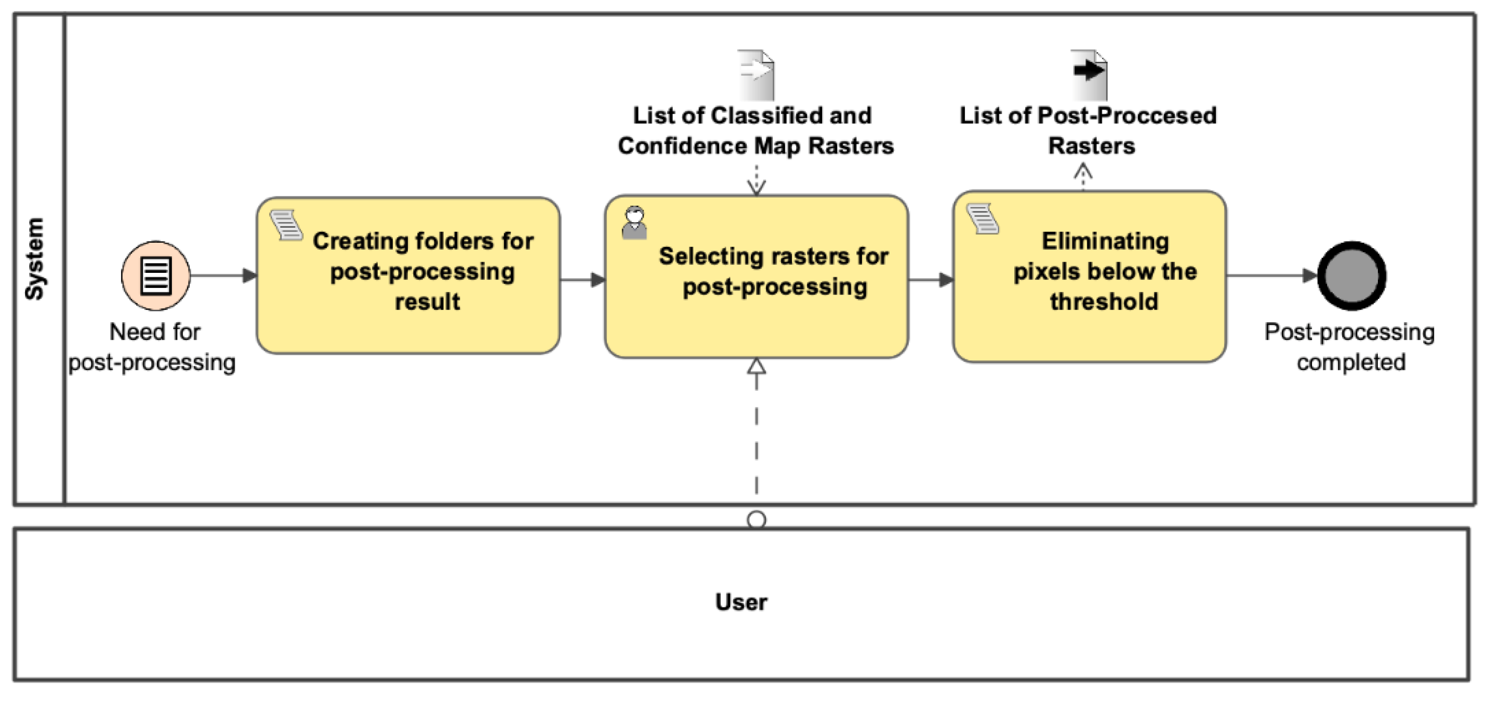
3.4. Satellite Data Post-Processing

Following the classification stage, a confidence-based filtering process was applied. Pixels with classification probabilities below a defined threshold were reclassified as “Unclassified” in order to minimize misclassification errors. Additionally, spatial smoothing techniques were applied to reduce noise and enhance the consistency of classification results.

The final classification output was validated using independent ground truth datasets and accuracy assessment metrics. This post-processing approach ensured that the final classification maps were both accurate and reliable for practical applications.

The subsequent post-processing operational steps are presented in Figure 7.

4. Results

This section presents the results of the experiment. To conduct an experiment on Sentinel-2 data classification using the proposed approach, a prototype was developed. The prototype ensures that the steps outlined in the method are implemented. The results obtained are presented separately for each step of the method.

4.1. Satellite Data Acquisition Results

During this phase, approximately 300 GB of Sentinel-2 (S2) satellite data was successfully acquired in the archived packages. These packages contained JPEG2000 (.jp2) file format satellite images. Each Sentinel-2 band was downloaded individually and then stored securely on a local storage system. After the download process was completed successfully, all archives were extracted, and unnecessary files were subsequently removed.

The dataset encompasses observations from 2022 to 2024, effectively capturing seasonal variations across the Lithuanian territory. The analyzed Sentinel-2 tiles were systematically categorized into ethnographic regions of Lithuania, facilitating easier territorial traceability. The ones that were analyzed are presented in

Table 2. Sentinel-2 tiles used in the experiment.

Region	Sentinel-2 Tiles
Žemaitija	34UDG, 34VDH, 34UEG, 34VEH
Aukštaitija	34VFH, 34UFG, 35VLC, 35ULB, 35UMB, 35VMC
Suvalkija	34UFF, 34UFE, 35ULA, 34UGE
Dzūkija	35ULV, 35UMA, 35UMV

.

An example of the S2 band is presented in Figure 8.

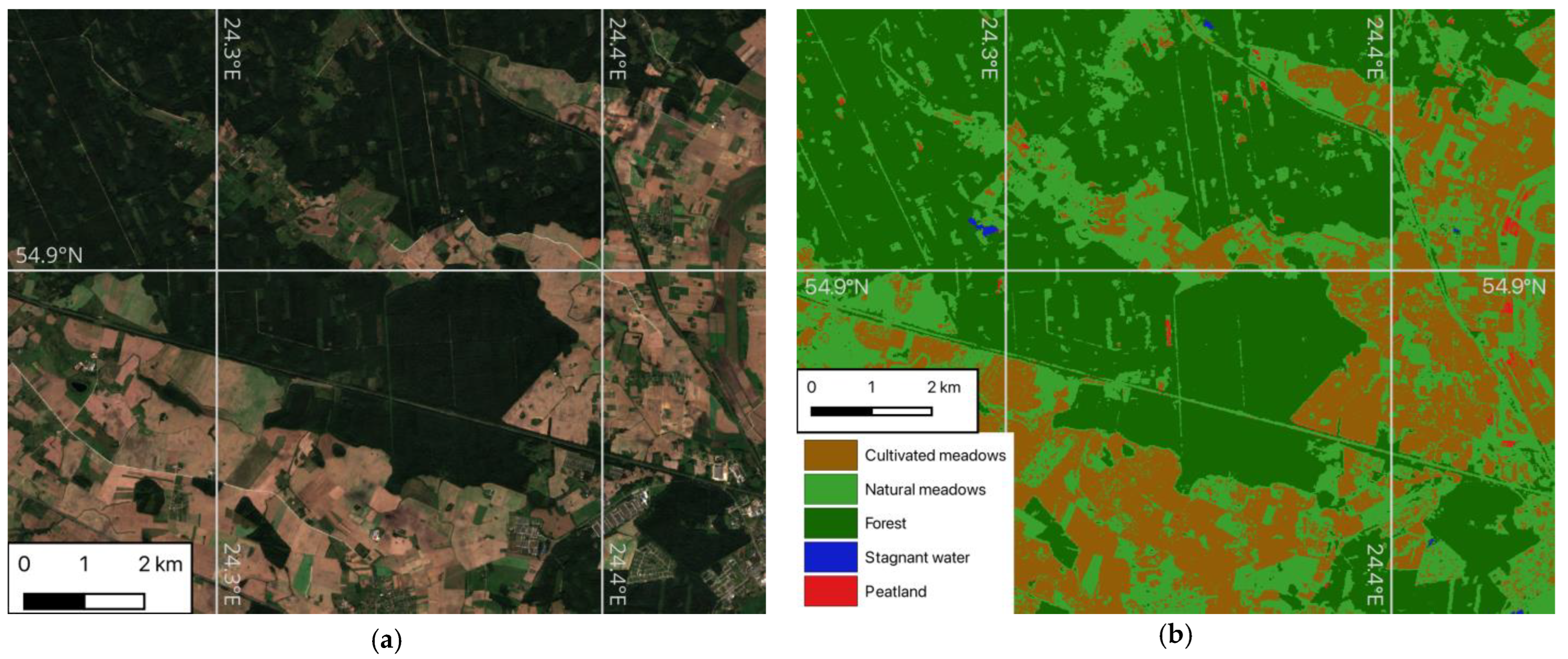
4.2. Pre-Processing Results

The results of the pre-processing stage are not easily tested or measured. It was observed that the satellite image layers were combined into a single image, indices were calculated, clouds were removed based on the Scene Classification Layer (SCL) and cloud interpolation was performed to obtain the best possible satellite images before proceeding to classification. It is therefore concluded that the outcomes of the aforementioned pre-processing are of a high standard and meet the objectives set out at the project’s inception.

The most verifiable pre-processing stage is the cloud interpolation stage, whereby an optimal satellite image is generated for each S2 geographic unit (tile) from all images acquired within a defined period (no longer than one month). To facilitate comprehension, the selection of interpolation cases was based on exceedingly high cloud cover, with the objective of enhancing the visibility of pixel swapping. For illustrative purposes, Figure 9 and Figure 10 present examples of the satellite images before and after cloud interpolation, respectively.

4.3. Classification Results and Reached Accuracy

4.3.1. Most Accurate Classifier

The literature analysis (see Section 2) has demonstrated that the most accurate algorithm, as determined by other scientific studies, is RF. Nevertheless, we have compared the results obtained from RF with those from the other two algorithms (i.e., Support Vector Machine (SVM) and K-Nearest Neighbors (KNN)) to determine which one is the most suitable for the case of the Baltic countries.

According to [66,67,68], the optimal hyperparameter search was performed for each classification algorithm. The optimal hyperparameters obtained for each algorithm are presented in

Table 3. Optimal hyperparameters for each classification algorithm.

Classifier	Optimal Hyperparameters
RF	n_estimators = 100, max_depth = 20, min_samples_leaf = 4, min_samples_split = 2
SVM	C = 0.1, gamma = scale, kernel = rbf
KNN	n_neighbors = 10, weights = uniform, p = 2

.

The classification accuracy averages achieved by each evaluated algorithm are summarized in

Table 4. Classification performance metrics for evaluated algorithms.

Classifier	Cohen’s Kappa	F1-Score	Recall	Precision
RF	89.23%	90.53%	90.86%	90.21%
SVM	86.23%	87.93%	88.16%	87.71%
KNN	84.73%	85.08%	85.36%	84.81%

.

As shown in Table 4, the classification results demonstrate significant performance differences among the evaluated algorithms. These differences can be attributable to variations in both model architecture and optimized hyperparameter configurations. The Random Forest (RF) classifier demonstrated the highest level of validation performance, highlighting its reliability and ability to identify complex, non-linear relationships in the feature space through ensemble learning and deep tree structures. The Support Vector Machine (SVM), utilizing an RBF kernel with a soft margin, performed comparably well, highlighting its efficacy in managing high-dimensional data and delineating non-linear class boundaries. Although the K-Nearest Neighbors (KNN) algorithm demonstrated slightly lower performance, its straightforward approach and reliance on local neighborhood structures still yielded competitive results. The findings indicate that ensemble-based methods, particularly RF, are highly suitable for land cover classification tasks using multi-spectral satellite imagery. SVM and KNN offer viable alternatives when considering computational constraints and data complexity.

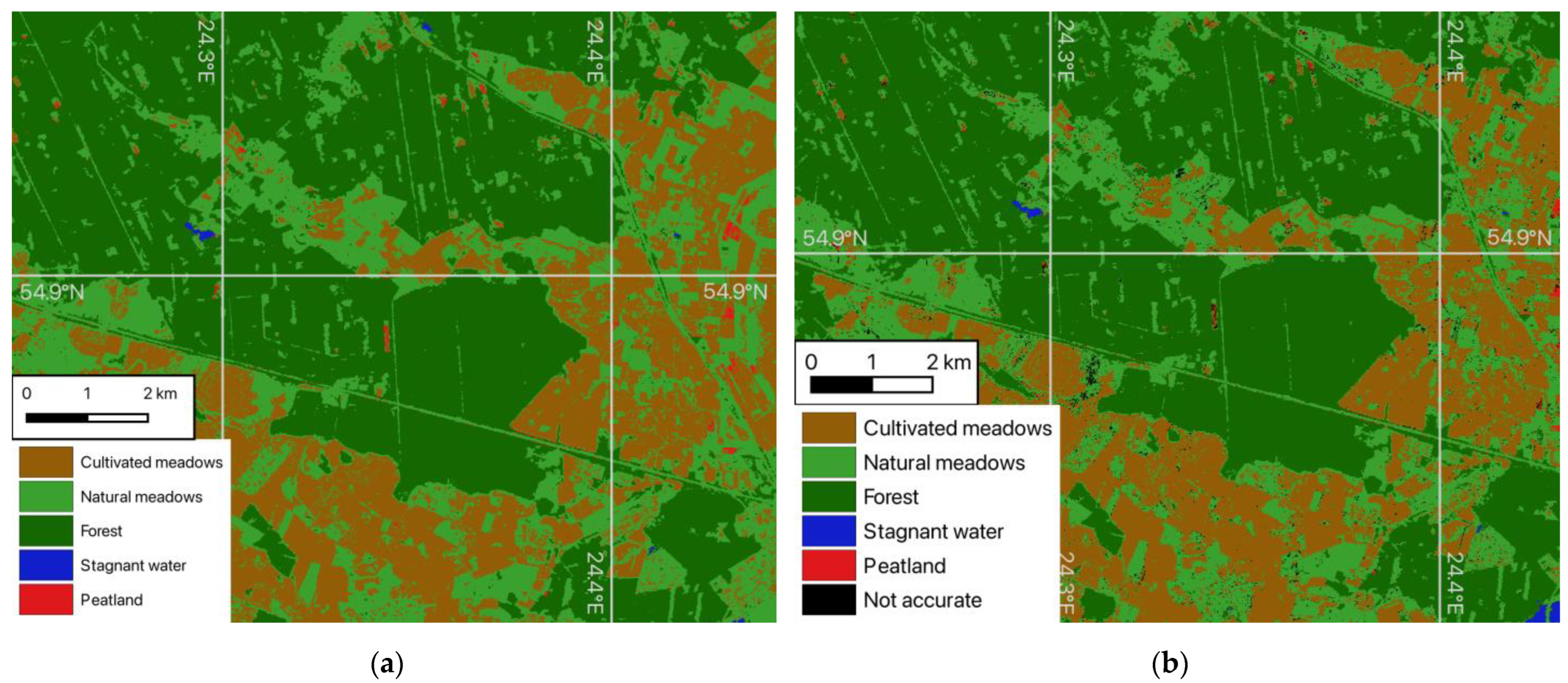
4.3.2. Final Classification Results

One of the key additional findings was that the inclusion of cloud interpolation significantly improved classification consistency in cloud-prone areas. The ability to reconstruct missing data from temporal information allowed the model to maintain high accuracy even in challenging atmospheric conditions. This approach ensured that cloud cover did not significantly affect classification results, making the method more suitable for operational land monitoring.

Additionally, the proposed method significantly outperformed traditional classification approaches by reducing misclassification due to seasonal variations in land use. Traditional methods often struggle with land cover transitions that occur over time, such as crop growth and deforestation. By incorporating vegetation indices and cloud handling mechanisms, the developed classification approach improved the differentiation of land use classes over multiple seasons, minimizing classification errors caused by spectral similarities between different land types. The input and output examples of the satellite image classification are shown in Figure 11.

Computational performance was also evaluated, showing that the classifier was efficient in processing large datasets while maintaining accuracy. Increasing the number of estimators in the Random Forest model improved classification performance but also increased processing time. A balance was achieved by optimizing hyperparameters to ensure both computational feasibility and classification accuracy. Further analysis of confidence maps revealed that some land use classes had higher classification uncertainty, especially in cases of spectral overlap. Refining the training datasets and incorporating additional contextual information could further improve the model’s performance in these ambiguous cases. The final results obtained are presented in

Table 5. Experiment accuracy results (overall accuracy (OA)).

Month	OA	Precision	Recall	F1	Cohen’s Kappa
April	90.45%	92.69%	91.45%	92.07%	90.96%
May	91.67%	92.28%	90.59%	91.43%	90.05%
June	90.40%	93.55%	90.40%	91.95%	88.50%
July	93.97%	97.20%	92.97%	95.04%	93.62%
August	90.61%	91.10%	90.61%	90.85%	90.03%
September	90.06%	96.26%	90.06%	93.06%	89.69%
October	93.13%	93.43%	93.13%	93.28%	90.13%

.

As shown in Table 5, the proposed method guarantees a classification accuracy of more than 90%, except for the months of June and September, where the results of the Cohen Kappa index indicate an accuracy of less than 90%. However, this deficiency is negligible.

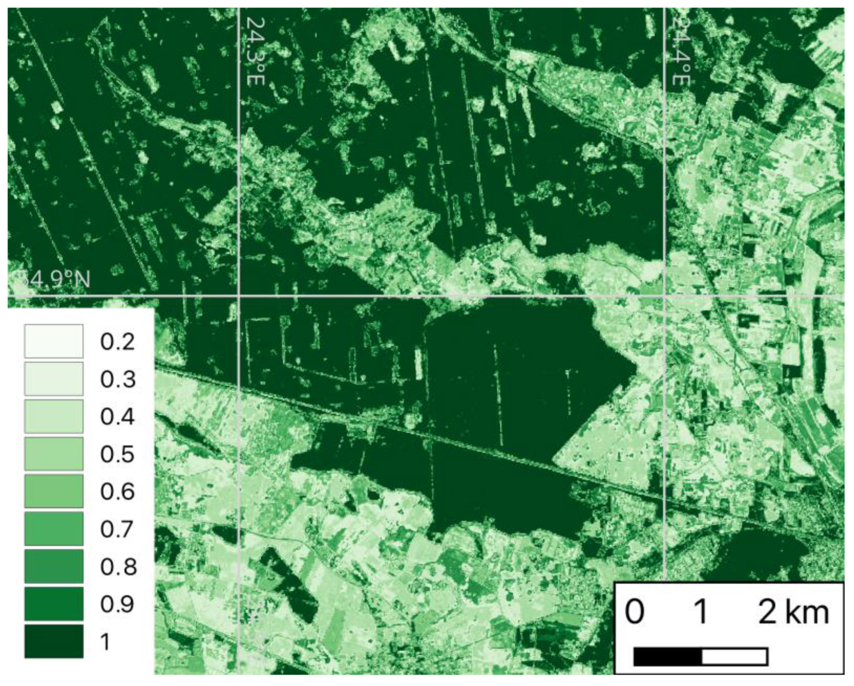
4.4. Post-Processing Results

After obtaining the classification results and conducting a detailed analysis, values were manually determined to set confidence thresholds, below which a pixel is considered unreliable and assigned to the “Unclassified” class. Figure 12 presents an example of a confidence map, which is utilized for the elimination of pixels below the defined threshold.

The figures illustrating the operation of the satellite image post-processing algorithm, both prior to and subsequent to the processing, are presented in Figure 13.

The confidence limits established by the post-processing experiments are presented in

Table 6. Post-processing thresholds after experiments (class code (CC), confidence value (CV)).

Land Use Class	CC	Month
		April	May	June	July	August	September	October
		CV	CV	CV	CV	CV	CV	CV
Arable land	11	0.3	0.32	-	-	0.26	0.38	0.32
Fallow	12	-	-	0.41	0.43	-	-	-
Stubble	13	-	-	-	-	0.47	-	-
Winter cereals	14	-	0.3	-	-	-	-	-
Intermediate crops	15	-	-	-	-	-	-	0.46
Intensive cultivated crops	16	-	0.37	0.49	0.4	0.55	-	-
Natural meadows	21	0.36	0.36	0.29	0.29	0.45	0.46	0.55
Forest	31	0.3	0.3	0.39	0.39	0.31	0.46	0.4
Stagnant Water	41	0.25	0.25	0.25	0.34	0.25	0.25	0.25
Urban areas	51	0.43	0.43	0.58	0.68	0.39	0.63	0.68
Sand dunes	61	0.54	0.54	0.48	0.48	0.25	0.3	0.5
Peatlands	62	-	0.5	0.39	0.39	0.39	0.53	0.3

(-)—Not analyzed. During different seasons not all classes appear, i.e., in June there is no stubble.

.

5. Discussion

Finally, in this section, we summarize and discuss our obtained results regarding our previously defined research aim to improve the assessment of land cover changes by proposing a hybrid ML, cloud interpolation, and vegetation indices-based approach.

As indicated by the findings of the literature review, the rapid development of artificial intelligence technologies and the increasing availability of high-resolution satellite data are enabling the efficient monitoring and management of land resources. However, the classification of land use remains challenging due to the variability of spectral characteristics, seasonal changes, regionality, and cloud interference. Consequently, the currently analyzed methods and approaches are unable to achieve the necessary level of accuracy when classifying land resources that are subject to dynamic change due to environmental conditions.

This paper proposes a hybrid ML, cloud interpolation, and vegetation/water indices-based approach for the classification of Sentinel-2 satellite imagery. The proposed approach offers several key advantages. First, it allows the filtering of satellite images using the cloud percentage, cloud removal using cloud interpolation and spectral index. Second, a Random Forest algorithm is employed to assign land use labels. Finally, classification results are refined by filtering out low-confidence predictions and improving spatial consistency.

The implemented approach and conducted experiments demonstrated that the hybrid approach significantly enhanced classification accuracy and robustness [4,16,22]. Our findings align with previous research [4,16,23], confirming the Random Forest classifier’s suitability and its notable adaptability to spectral variability, seasonal changes, and common challenges such as cloud cover interference. It is important to note that cloud interpolation and vegetation or water indices (e.g., NDTI, NDVIre, and MNDWI) included in the proposed approach demonstrated improvement in classification reliability, echoing the results of previous studies that highlight the advantage of integrating spectral indices for more precise feature extraction from Sentinel-2 data [2,5,61]. Specifically, the implemented cloud interpolation method allowed us to effectively mitigate cloud interference, which was identified as a key factor for the improvements in the literature [6,59,69].

Moreover, the selected Random Forest classifier parameters—maximum tree depth set at 20, estimators at 100, min samples split at 2 and finally min samples leaf at 4—yielded optimal balance in accuracy and computational efficiency. This finding aligns with previous research indicating that parameter tuning significantly impacts classifier performance [22,25,62]. Furthermore, the post-processing thresholds established in accordance with the confidence maps effectively filtered out low-confidence predictions, thereby enhancing the reliability of classification outputs. This methodological improvement aligns with insights from previous works, underscoring the value of confidence-based post-processing in satellite image classification [6,59,70].

These findings support the hypothesis that integrating cloud interpolation, spectral indices, and ML enhances the accuracy of land use classification under dynamic environmental conditions. The proposed hybrid method is robust, with implications that extend beyond the Lithuanian context. Its potential applications include regions with high cloud coverage or similar environmental variability [6,7,8,69]. For future research, expanding training datasets temporally and spatially, incorporating data from diverse satellite missions, or exploring fusion with synthetic aperture radar (SAR) imagery, may further enhance classification accuracy and generalizability. Additionally, testing this approach in other geographical contexts, as suggested by [9,71] would help validate the adaptability and effectiveness of the methodology more broadly. The study confirms that integrating pre-processing enhancements such as cloud removal and spectral indices improves classification accuracy. This indicates that the objective has been successfully met.

Limitations of the Research

However, several limitations remain to be considered. One of the primary challenges is in distinguishing visually similar land use types, particularly during seasonal transitions. Some land use classes, such as fallow fields and natural meadows, exhibit spectral similarities that pose difficulties in classification. Future research should explore the integration of temporal data analysis to mitigate classification errors caused by seasonal variations.

Another limitation is the reliance on manually labeled training data. Although high-quality labeled datasets were sourced from governmental agencies, which represent exact land use, there remains potential for error when creating training and validation sets due to human error. The incorporation of semi-supervised or unsupervised learning techniques has the potential to enhance the system independency of labeled data and improve classification robustness.

Furthermore, while cloud interpolation is an effective method for enhancing data availability, it is important to note that it may introduce artifacts when cloud coverage is extensive. This can affect classification accuracy, particularly in regions with persistent cloud cover. Future work should explore deep learning-based gap-filling techniques to further enhance interpolation accuracy.

Another key consideration is computational efficiency. The proposed method is accurate, but it requires substantial computational resources due to the high resolution of the imagery and the large size of the dataset. Optimization strategies, such as model pruning and quantization, should be explored to improve the efficiency of classification algorithms without compromising accuracy.

The present study is confined to Lithuania, a setting that is representative of the climate and land use characteristics of the Baltic region. However, it is expected that the methodological framework will be extended to other regions with similar environmental conditions. In Europe, beyond the immediate Baltic neighbors of Latvia and Estonia, countries such as Finland, Sweden, and even parts of Poland or the northern coastal areas of Germany have comparable transitional continental climates with significant seasonal variability. In North America, regions within Canada with analogous mid-latitude conditions further underline the potential transferability of the approach. In addition, several regions in Asia, including northern Japan (particularly Hokkaido), parts of South Korea and parts of northeast China, exhibit environmental conditions similar to those observed in the Baltic region. While these findings are encouraging, further empirical validation is necessary to establish the robustness of the model across the wider range of climates, land use types and instances of persistent cloud cover found in these diverse but climatically analogous regions. All those works are left for further research.

6. Conclusions and Future Works

This study demonstrates the feasibility of using Sentinel-2 imagery and ML techniques for land use classification. The proposed methodology, incorporating cloud interpolation and vegetation indices, has been successfully implemented to enhance the accuracy of classification in Lithuania. Furthermore, these findings contribute to the development of automated, scalable land monitoring systems applicable to broader geographic regions. However, additional research is necessary to fully explore this potential.

Future research should focus on enhancing classification robustness by integrating deep learning techniques such as Convolutional Neural Networks (CNNs) and Transformer-based models. Additionally, exploring multi-temporal analysis has the potential to enhance classification accuracy by incorporating seasonal variations into the model. Implementing semi-supervised learning can reduce the need for manually labeled datasets and improve adaptability to different regions. In order to reduce processing time and improve efficiency for large-scale applications, it is advisable to explore computational optimizations. Finally, testing the proposed methodology in diverse geographic regions would help assess its generalizability and refine the classification approach for broader applications.

References

1. Flohr, P.; Bradbury, J.; ten Harkel, L. Tracing the Patterns: Fields, Villages, and Burial Places in Lebanon. Levant 2021, 53, 315–335. [Google Scholar] [CrossRef]
2. Marchetti, G.; Bizzi, S.; Belletti, B.; Lastoria, B.; Comiti, F.; Carbonneau, P.E. Mapping Riverbed Sediment Size from Sentinel-2 Satellite Data. Earth Surf. Process. Landf. 2022, 47, 2544–2559. [Google Scholar] [CrossRef]
3. Zhang, T.X.; Su, J.Y.; Liu, C.J.; Chen, W.H. Potential Bands of Sentinel-2A Satellite for Classification Problems in Precision Agriculture. Int. J. Autom. Comput. 2019, 16, 16–26. [Google Scholar] [CrossRef]
4. Dobrinić, D.; Gašparović, M.; Medak, D. Sentinel-1 and 2 Time-Series for Vegetation Mapping Using Random Forest Classification: A Case Study of Northern Croatia. Remote Sens. 2021, 13, 2321. [Google Scholar] [CrossRef]
5. Xue, H.; Xu, X.; Zhu, Q.; Yang, G.; Long, H.; Li, H.; Yang, X.; Zhang, J.; Yang, Y.; Xu, S.; et al. Object-Oriented Crop Classification Using Time Series Sentinel Images from Google Earth Engine. Remote Sens. 2023, 15, 1353. [Google Scholar] [CrossRef]
6. Fan, Z.; Zhan, T.; Gao, Z.; Li, R.; Liu, Y.; Zhang, L.; Jin, Z.; Xu, S. Land Cover Classification of Resources Survey Remote Sensing Images Based on Segmentation Model. IEEE Access 2022, 10, 56267–56281. [Google Scholar] [CrossRef]
7. Eisfelder, C.; Boemke, B.; Gessner, U.; Sogno, P.; Alemu, G.; Hailu, R.; Mesmer, C.; Huth, J. Cropland and Crop Type Classification with Sentinel-1 and Sentinel-2 Time Series Using Google Earth Engine for Agricultural Monitoring in Ethiopia. Remote Sens. 2024, 16, 866. [Google Scholar] [CrossRef]
8. Farhadiani, R.; Homayouni, S.; Bhattacharya, A.; Mahdianpari, M. Crop Classification Using Multi-Temporal RADARSAT Constellation Mission Compact Polarimetry SAR Data. Can. J. Remote Sens. 2024, 50, 2384883. [Google Scholar] [CrossRef]
9. Wang, Y.; Jin, S.; Dardanelli, G. Vegetation Classification and Evaluation of Yancheng Coastal Wetlands Based on Random Forest Algorithm from Sentinel-2 Images. Remote Sens. 2024, 16, 1124. [Google Scholar] [CrossRef]
10. Roy, D.P.; Li, J.; Zhang, H.K.; Yan, L. Best Practices for the Reprojection and Resampling of Sentinel-2 Multi Spectral Instrument Level 1C Data. Remote Sens. Lett. 2016, 7, 1023–1032. [Google Scholar] [CrossRef]
11. Arp, L.; Hoos, H.; van Bodegom, P.; Francis, A.; Wheeler, J.; van Laar, D.; Baratchi, M. Training-Free Thick Cloud Removal for Sentinel-2 Imagery Using Value Propagation Interpolation. ISPRS J. Photogramm. Remote Sens. 2024, 216, 168–184. [Google Scholar] [CrossRef]
12. Meraner, A.; Ebel, P.; Zhu, X.X.; Schmitt, M. Cloud Removal in Sentinel-2 Imagery Using a Deep Residual Neural Network and SAR-Optical Data Fusion. ISPRS J. Photogramm. Remote Sens. 2020, 166, 333–346. [Google Scholar] [CrossRef]
13. Bill Donatien, L.M.; Biona Clobite, B.; Lemvo Meris Midel, M. Comparing Sentinel-2 and Landsat 9 for Land Use and Land Cover Mapping Assessment in the North of Congo Republic: A Case Study in Sangha Region. Int. J. Remote Sens. 2024, 45, 8015–8036. [Google Scholar] [CrossRef]
14. Trevisiol, F.; Mandanici, E.; Pagliarani, A.; Bitelli, G. Evaluation of Landsat-9 Interoperability with Sentinel-2 and Landsat-8 over Europe and Local Comparison with Field Surveys. ISPRS J. Photogramm. Remote Sens. 2024, 210, 55–68. [Google Scholar] [CrossRef]
15. Poussin, C.; Peduzzi, P.; Giuliani, G. Snow Observation from Space: An Approach to Improving Snow Cover Detection Using Four Decades of Landsat and Sentinel-2 Imageries across Switzerland. Sci. Remote Sens. 2025, 11, 100182. [Google Scholar] [CrossRef]
16. Cuypers, S.; Nascetti, A.; Vergauwen, M. Land Use and Land Cover Mapping with VHR and Multi-Temporal Sentinel-2 Imagery. Remote Sens. 2023, 15, 2501. [Google Scholar] [CrossRef]
17. Bio Nikki Sarè, S.B.; Gaetano, R.; Interdonato, R.; Hountondji, Y.C.; Ienco, D.; Dantas, C.F. Joint Cloud Removal and Classification of Sentinel-2 Image Time Series for Agricultural Land Cover Mapping in Northern Benin. In Proceedings of the IGARSS 2024—2024 IEEE International Geoscience and Remote Sensing Symposium, Athens, Greece, 7–12 July 2024; pp. 4824–4827. [Google Scholar]
18. Huang, H.; Roy, D.P.; De Lemos, H.; Qiu, Y.; Zhang, H.K. A Global Swin-Unet Sentinel-2 Surface Reflectance-Based Cloud and Cloud Shadow Detection Algorithm for the NASA Harmonized Landsat Sentinel-2 (HLS) Dataset. Sci. Remote Sens. 2025, 11, 100213. [Google Scholar] [CrossRef]
19. Patel, P.N.; Jiang, J.H.; Gautam, R.; Gadhavi, H.; Kalashnikova, O.; Garay, M.J.; Gao, L.; Xu, F.; Omar, A. A Remote Sensing Algorithm for Vertically Resolved Cloud Condensation Nuclei Number Concentrations from Airborne and Spaceborne Lidar Observations. Atmos. Chem. Phys. 2024, 24, 2861–2883. [Google Scholar] [CrossRef]
20. Zhou, J.; Luo, X.; Rong, W.; Xu, H. Cloud Removal for Optical Remote Sensing Imagery Using Distortion Coding Network Combined with Compound Loss Functions. Remote Sens. 2022, 14, 3452. [Google Scholar] [CrossRef]
21. Wang, Q.; Wang, L.; Zhu, X.; Ge, Y.; Tong, X.; Atkinson, P.M. Remote Sensing Image Gap Filling Based on Spatial-Spectral Random Forests. Sci. Remote Sens. 2022, 5, 100048. [Google Scholar] [CrossRef]
22. Kumar, A.; Abhishek, K.; Kumar Singh, A.; Nerurkar, P.; Chandane, M.; Bhirud, S.; Patel, D.; Busnel, Y. Multilabel Classification of Remote Sensed Satellite Imagery. Trans. Emerg. Telecommun. Technol. 2021, 32, e3988. [Google Scholar] [CrossRef]
23. Albertini, C.; Gioia, A.; Iacobellis, V.; Petropoulos, G.P.; Manfreda, S. Assessing Multi-Source Random Forest Classification and Robustness of Predictor Variables in Flooded Areas Mapping. Remote Sens. Appl. 2024, 35, 101239. [Google Scholar] [CrossRef]
24. Judah, A.; Hu, B. The Integration of Multi-Source Remotely Sensed Data with Hierarchically Based Classification Approaches in Support of the Classification of Wetlands. Can. J. Remote Sens. 2022, 48, 158–181. [Google Scholar] [CrossRef]
25. Ioannou, K. On the Identification of Agroforestry Application Areas Using Object-Oriented Programming. Agriculture 2023, 13, 164. [Google Scholar] [CrossRef]
26. Alhassan, V.; Henry, C.; Ramanna, S.; Storie, C. A Deep Learning Framework for Land-Use/Land-Cover Mapping and Analysis Using Multispectral Satellite Imagery. Neural Comput. Appl. 2020, 32, 8529–8544. [Google Scholar] [CrossRef]
27. Hejmanowska, B.; Kramarczyk, P. Assessing Land Cover Changes Using the LUCAS Database and Sentinel Imagery: A Comparative Analysis of Accuracy Metrics. Appl. Sci. 2025, 15, 240. [Google Scholar] [CrossRef]
28. Li, C.; Li, H.; Zhou, Y.; Wang, X. Detailed Land Use Classification in a Rare Earth Mining Area Using Hyperspectral Remote Sensing Data for Sustainable Agricultural Development. Sustainability 2024, 16, 3582. [Google Scholar] [CrossRef]
29. Perregrini, D.; Casella, V. Land Use Recognition by Applying Fuzzy Logic and Object-Based Classification to Very High Resolution Satellite Images. Remote Sens. 2024, 16, 2273. [Google Scholar] [CrossRef]
30. Shao, M.; Xie, X.; Li, K.; Li, C.; Zhou, X. Semantic-Enhanced Foundation Model for Coastal Land Use Recognition from Optical Satellite Images. Appl. Sci. 2024, 14, 9431. [Google Scholar] [CrossRef]
31. Holloway, J.; Helmstedt, K.J.; Mengersen, K.; Schmidt, M. A Decision Tree Approach for Spatially Interpolating Missing Land Cover Data and Classifying Satellite Images. Remote Sens. 2019, 11, 1796. [Google Scholar] [CrossRef]
32. Souza, F.E.S.d.; Rodrigues, J.I.d.J. Evaluation of Machine Learning Algorithms in the Classification of Multispectral Images from the Sentinel-2A/2B Orbital Sensor for Mapping the Environmental Dynamics of Ria Formosa (Algarve, Portugal). ISPRS Int. J. Geo-Inf. 2023, 12, 361. [Google Scholar] [CrossRef]
33. Kamenova, I.; Chanev, M.; Dimitrov, P.; Filchev, L.; Bonchev, B.; Zhu, L.; Dong, Q. Crop Type Mapping and Winter Wheat Yield Prediction Utilizing Sentinel-2: A Case Study from Upper Thracian Lowland, Bulgaria. Remote Sens. 2024, 16, 1144. [Google Scholar] [CrossRef]
34. Kluczek, M.; Zagajewski, B.; Kycko, M. Combining Multitemporal Optical and Radar Satellite Data for Mapping the Tatra Mountains Non-Forest Plant Communities. Remote Sens. 2024, 16, 1451. [Google Scholar] [CrossRef]
35. Kluczek, M.; Zagajewski, B.; Zwijacz-Kozica, T. Mountain Tree Species Mapping Using Sentinel-2, PlanetScope, and Airborne HySpex Hyperspectral Imagery. Remote Sens. 2023, 15, 844. [Google Scholar] [CrossRef]
36. Aliabad, F.A.; Malamiri, H.R.G.; Shojaei, S.; Sarsangi, A.; Ferreira, C.S.S.; Kalantari, Z. Investigating the Ability to Identify New Constructions in Urban Areas Using Images from Unmanned Aerial Vehicles, Google Earth, and Sentinel-2. Remote Sens. 2022, 14, 3227. [Google Scholar] [CrossRef]
37. Bebie, M.; Cavalaris, C.; Kyparissis, A. Assessing Durum Wheat Yield through Sentinel-2 Imagery: A Machine Learning Approach. Remote Sens. 2022, 14, 3880. [Google Scholar] [CrossRef]
38. Zhang, H.; He, J.; Chen, S.; Zhan, Y.; Bai, Y.; Qin, Y. Comparing Three Methods of Selecting Training Samples in Supervised Classification of Multispectral Remote Sensing Images. Sensors 2023, 23, 8530. [Google Scholar] [CrossRef]
39. Pokhariya, H.S.; Singh, D.P.; Prakash, R. Evaluation of Different Machine Learning Algorithms for LULC Classification in Heterogeneous Landscape by Using Remote Sensing and GIS Techniques. Eng. Res. Express 2023, 5, 045052. [Google Scholar] [CrossRef]
40. Kycko, M.; Zagajewski, B.; Kluczek, M.; Tardà, A.; Pineda, L.; Palà, V.; Corbera, J. Sentinel-2 and AISA Airborne Hyperspectral Images for Mediterranean Shrubland Mapping in Catalonia. Remote Sens. 2022, 14, 5531. [Google Scholar] [CrossRef]
41. Ren, C.; Jiang, H.; Xi, Y.; Liu, P.; Li, H. Quantifying Temperate Forest Diversity by Integrating GEDI LiDAR and Multi-Temporal Sentinel-2 Imagery. Remote Sens. 2023, 15, 375. [Google Scholar] [CrossRef]
42. Arfa, A.; Minaei, M. Utilizing Multitemporal Indices and Spectral Bands of Sentinel-2 to Enhance Land Use and Land Cover Classification with Random Forest and Support Vector Machine. Adv. Space Res. 2024, 74, 5580–5590. [Google Scholar] [CrossRef]
43. Keskes, M.I.; Mohamed, A.H.; Borz, S.A.; Niţă, M.D. Improving National Forest Mapping in Romania Using Machine Learning and Sentinel-2 Multispectral Imagery. Remote Sens. 2025, 17, 715. [Google Scholar] [CrossRef]
44. Caputi, E.; Delogu, G.; Patriarca, A.; Perretta, M.; Mancini, G.; Boccia, L.; Recanatesi, F.; Ripa, M.N. Comparison of Tree Typologies Mapping Using Random Forest Classifier Algorithm of PRISMA and Sentinel-2 Products in Different Areas of Central Italy. Remote Sens. 2025, 17, 356. [Google Scholar] [CrossRef]
45. Wang, Z. Spatial Differentiation Characteristics of Rural Areas Based on Machine Learning and GIS Statistical Analysis—A Case Study of Yongtai County, Fuzhou City. Sustainability 2023, 15, 4367. [Google Scholar] [CrossRef]
46. Stachura, G.; Ustrnul, Z.; Sekuła, P.; Bochenek, B.; Kolonko, M.; Szczęch-Gajewska, M. Machine Learning Based Post-Processing of Model-Derived near-Surface Air Temperature—A Multimodel Approach. Q. J. R. Meteorol. Soc. 2024, 150, 618–631. [Google Scholar] [CrossRef]
47. Lemenkova, P. GRASS GIS Scripts for Satellite Image Analysis by Raster Calculations Using Modules r.Mapcalc, d.Rgb, r.Slope.Aspect. Teh. Vjesn. 2022, 29, 1956–1963. [Google Scholar] [CrossRef]
48. Ole Ørka, H.; Gailis, J.; Vege, M.; Gobakken, T.; Hauglund, K. Analysis-Ready Satellite Data Mosaics from Landsat and Sentinel-2. IEEE J. Sel. Top. Appl. Earth Obs. Remote Sens. 2013, 6, 2088–2101. [Google Scholar]
49. Schürz, M.; Grigoropoulou, A.; García Márquez, J.; Torres-Cambas, Y.; Tomiczek, T.; Floury, M.; Bremerich, V.; Schürz, C.; Amatulli, G.; Grossart, H.P.; et al. Hydrographr: An R Package for Scalable Hydrographic Data Processing. Methods Ecol. Evol. 2023, 14, 2953–2963. [Google Scholar] [CrossRef]
50. Juhász, L.; Xu, J.; Parkinson, R.W. Beyond the Tide: A Comprehensive Guide to Sea-Level-Rise Inundation Mapping Using FOSS4G. Geomatics 2023, 3, 522–540. [Google Scholar] [CrossRef]
51. Logan, T.L.; Smyth, M.M.; Calef, F.J. Planetary Orbital Mapping and Mosaicking (POMM) Integrated Open Source Software Environment. Astron. Comput. 2024, 46, 100788. [Google Scholar] [CrossRef]
52. Gonzalez, S.T.; Velez-Zea, A.; Barrera-Ramírez, J.F. High Performance Holographic Video Compression Using Spatio-Temporal Phase Unwrapping. Opt. Lasers Eng. 2024, 181, 108381. [Google Scholar] [CrossRef]
53. Kai, X.; Yuxiang, Z. Improving the Performance of 3D Image Model Compression Based on Optimized DEFLATE Algorithm. Sci. Rep. 2024, 14, 14899. [Google Scholar] [CrossRef] [PubMed]
54. Jeromel, A.; Žalik, B. An Efficient Lossy Cartoon Image Compression Method. Multimed. Tools Appl. 2020, 79, 433–451. [Google Scholar] [CrossRef]
55. Liu, C.; Huang, H.; Hui, F.; Zhang, Z.; Cheng, X. Fine-Resolution Mapping of Pan-Arctic Lake Ice-off Phenology Based on Dense Sentinel-2 Time Series Data. Remote Sens. 2021, 13, 2742. [Google Scholar] [CrossRef]
56. Psychalas, C.; Vlachos, K.; Moumtzidou, A.; Gialampoukidis, I.; Vrochidis, S.; Kompatsiaris, I. Towards a Paradigm Shift on Mapping Muddy Waters with Sentinel-2 Using Machine Learning. Sustainability 2023, 15, 13441. [Google Scholar] [CrossRef]
57. Shao, M.; Zou, Y. Multi-Spectral Cloud Detection Based on a Multi-Dimensional and Multi-Grained Dense Cascade Forest. J. Appl. Remote Sens. 2021, 15, 028507. [Google Scholar] [CrossRef]
58. Shepherd, J.D.; Schindler, J.; Dymond, J.R. Automated Mosaicking of Sentinel-2 Satellite Imagery. Remote Sens. 2020, 12, 3680. [Google Scholar] [CrossRef]
59. Farhadi, H.; Ebadi, H.; Kiani, A.; Asgary, A. Near Real-Time Flood Monitoring Using Multi-Sensor Optical Imagery and Machine Learning by GEE: An Automatic Feature-Based Multi-Class Classification Approach. Remote Sens. 2024, 16, 4454. [Google Scholar] [CrossRef]
60. Niazmardi, S.; Homayouni, S.; Safari, A.; McNairn, H.; Shang, J.; Beckett, K. Histogram-Based Spatio-Temporal Feature Classification of Vegetation Indices Time-Series for Crop Mapping. Int. J. Appl. Earth Obs. Geoinf. 2018, 72, 34–41. [Google Scholar] [CrossRef]
61. Sankaran, R.; Al-Khayat, J.A.; Chatting, M.E.; Sadooni, F.N.; Al-Kuwari, H.A.S. Retrieval of Suspended Sediment Concentration (SSC) in the Arabian Gulf Water of Arid Region by Sentinel-2 Data. Sci. Total Environ. 2023, 904, 166875. [Google Scholar] [CrossRef]
62. Terzi Türk, S.; Balçik, F. Rastgele Orman Algoritması ve Sentinel-2 MSI Ile Fındık Ekili Alanların Belirlenmesi: Piraziz Örneği. Geomatik 2023, 8, 91–98. [Google Scholar] [CrossRef]
63. Belayhun, M.; Chere, Z.; Abay, N.G.; Nicola, Y.; Asmamaw, A. Spatiotemporal Pattern of Water Hyacinth (Pontederia Crassipes) Distribution in Lake Tana, Ethiopia, Using a Random Forest Machine Learning Model. Front. Environ. Sci. 2024, 12, 1476014. [Google Scholar] [CrossRef]
64. Lee, J.; Kim, K.; Lee, K. Multi-Sensor Image Classification Using the Random Forest Algorithm in Google Earth Engine with KOMPSAT-3/5 and CAS500-1 Images. Remote Sens. 2024, 16, 4622. [Google Scholar] [CrossRef]
65. Casamitjana, M.; Torres-Madroñero, M.C.; Bernal-Riobo, J.; Varga, D. Soil Moisture Analysis by Means of Multispectral Images According to Land Use and Spatial Resolution on Andosols in the Colombian Andes. Appl. Sci. 2020, 10, 5540. [Google Scholar] [CrossRef]
66. Alshammari, T. Using Artificial Neural Networks with GridSearchCV for Predicting Indoor Temperature in a Smart Home. Eng. Technol. Appl. Sci. Res. 2024, 14, 13437–13443. [Google Scholar] [CrossRef]
67. Ahmad, G.N.; Fatima, H.; Ullah, S.; Saidi, A.S. Imdadullah Efficient Medical Diagnosis of Human Heart Diseases Using Machine Learning Techniques with and Without GridSearchCV. IEEE Access 2022, 10, 80151–80173. [Google Scholar] [CrossRef]
68. Vazirani, H.; Wu, X.; Srivastava, A.; Dhar, D.; Pathak, D. Highly Efficient JR Optimization Technique for Solving Prediction Problem of Soil Organic Carbon on Large Scale. Sensors 2024, 24, 7317. [Google Scholar] [CrossRef]
69. Anandakrishnan, J.; Sundaram, V.M.; Paneer, P. CERMF-Net: A SAR-Optical Feature Fusion for Cloud Elimination From Sentinel-2 Imagery Using Residual Multiscale Dilated Network. IEEE J. Sel. Top. Appl. Earth Obs. Remote Sens. 2024, 17, 11741–11749. [Google Scholar] [CrossRef]
70. Gu, X.; Angelov, P.P.; Zhang, C.; Atkinson, P.M. A Semi-Supervised Deep Rule-Based Approach for Complex Satellite Sensor Image Analysis. IEEE Trans. Pattern Anal. Mach. Intell. 2022, 44, 2281–2292. [Google Scholar] [CrossRef]
71. Rodríguez-Puerta, F.; Perroy, R.L.; Barrera, C.; Price, J.P.; García-Pascual, B. Five-Year Evaluation of Sentinel-2 Cloud-Free Mosaic Generation Under Varied Cloud Cover Conditions in Hawai’i. Remote Sens. 2024, 16, 4791. [Google Scholar] [CrossRef]
Figure 1. A schema of the hybrid ML, cloud interpolation, and vegetation indices-based approach.
Applsci 15 04765 g001
Figure 2. Detailed data acquisition schema. Dotted line—message flow; X—exclusive gateway; +—parallel gateway.
Applsci 15 04765 g002
Figure 3. Detailed representation of the satellite data download process. Dotted line—message flow; X—exclusive gateway; +—parallel gateway.
Applsci 15 04765 g003
Figure 4. Detailed representation of the satellite data pre-processing process. Dotted line—message flow; +—parallel gateway.
Applsci 15 04765 g004
Figure 5. Illustrative example of crop records combined with S2 data (collapsed legend).
Applsci 15 04765 g005
Figure 6. Detailed representation of the satellite data classification process. Dotted line—message flow; +—parallel gateway.
Applsci 15 04765 g006
Figure 7. Detailed representation of the satellite data post-processing process. Dotted line—message flow.
Applsci 15 04765 g007
Figure 8. S2 band 6 (B6)—vegetation red edge.
Applsci 15 04765 g008
Figure 9. Sentinel-2 satellite tiles examples. (a) Sentinel-2 tile (34UFF) from early August. (b) Sentinel-2 tile (34UFF) two days later.
Applsci 15 04765 g009
Figure 10. Output satellite image of the cloud interpolation algorithm.
Applsci 15 04765 g010
Figure 11. Input and output examples of the satellite image classification. (a) Input satellite image for the classification algorithm; (b) output satellite image of the classification algorithm (note: the legend presents only land use classes which appear in the analyzed region).
Applsci 15 04765 g011
Figure 12. An example of a confidence map.
Applsci 15 04765 g012
Figure 13. Example of post-processing process. (a) Input classified satellite image for post-processing. (b) Result (output) of post-processed satellite image.
Applsci 15 04765 g013